
Comparison of Hyperspectral Imaging and Near-Infrared Spectroscopy to Determine Nitrogen and Carbon Concentrations in Wheat

 ,
, 
 and
and
Abstract
:
1. Introduction
2. Materials and Methods
2.1. Experimental Design Overview
2.2. Sample Collection, Preparation and Wet Chemistry Analysis
2.3. Spectral Analysis of the Ground Wheat Samples
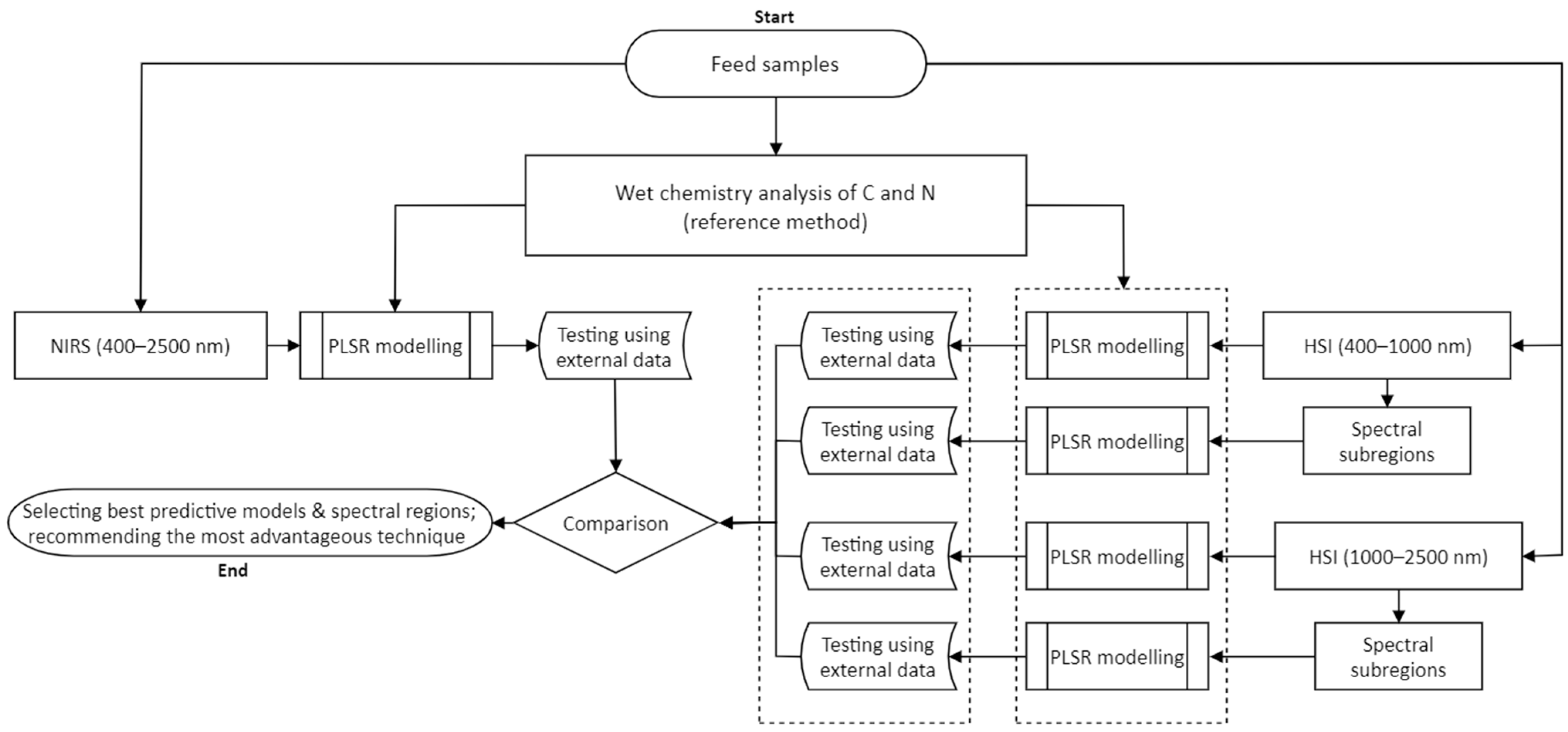
2.3.1. Acquisition of Spectral Reflectance Using NIRS and HSI
2.3.2. Hyperspectral Image Correction and Sample Identification
2.3.3. PLSR Model Development and Evaluation
2.3.4. Identification of the Important Spectral Regions
3. Results
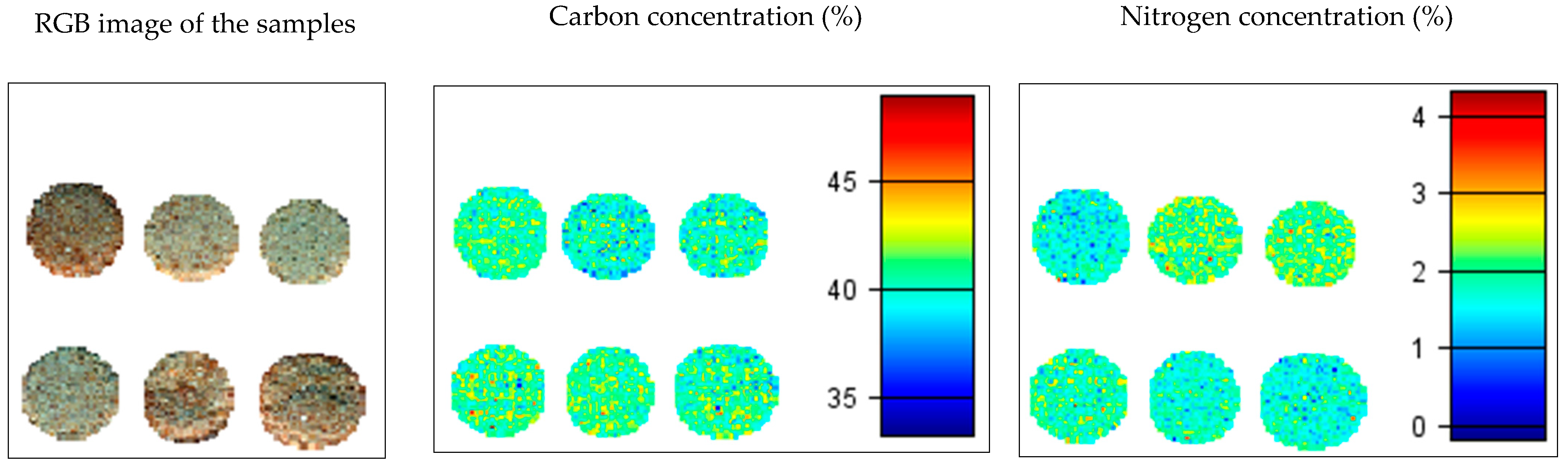
3.1. Descriptive Analysis
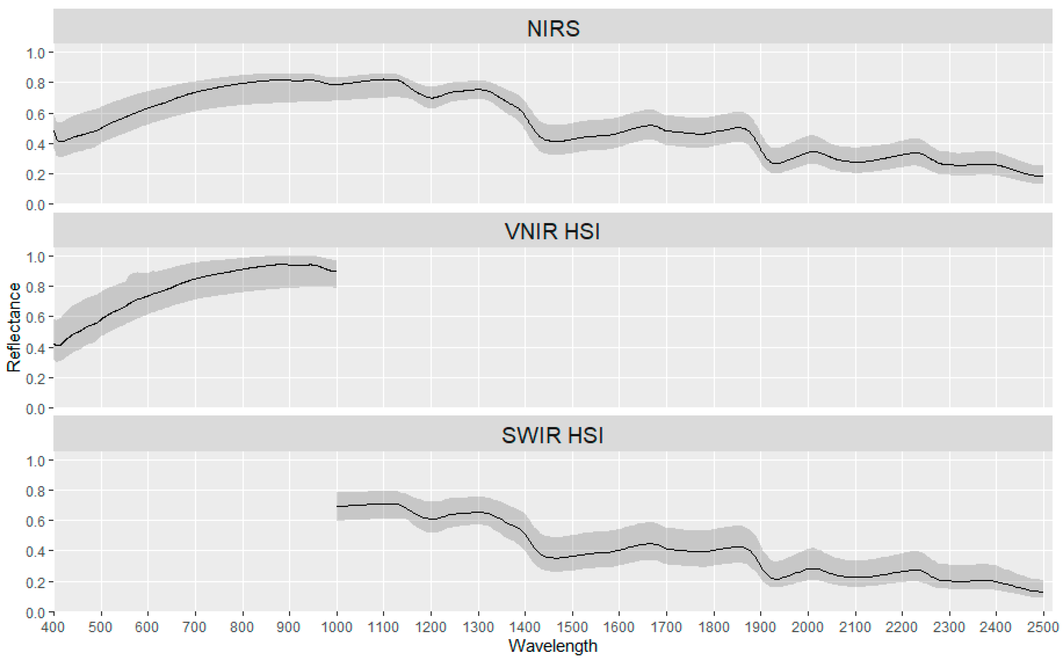
3.2. Spectral Features
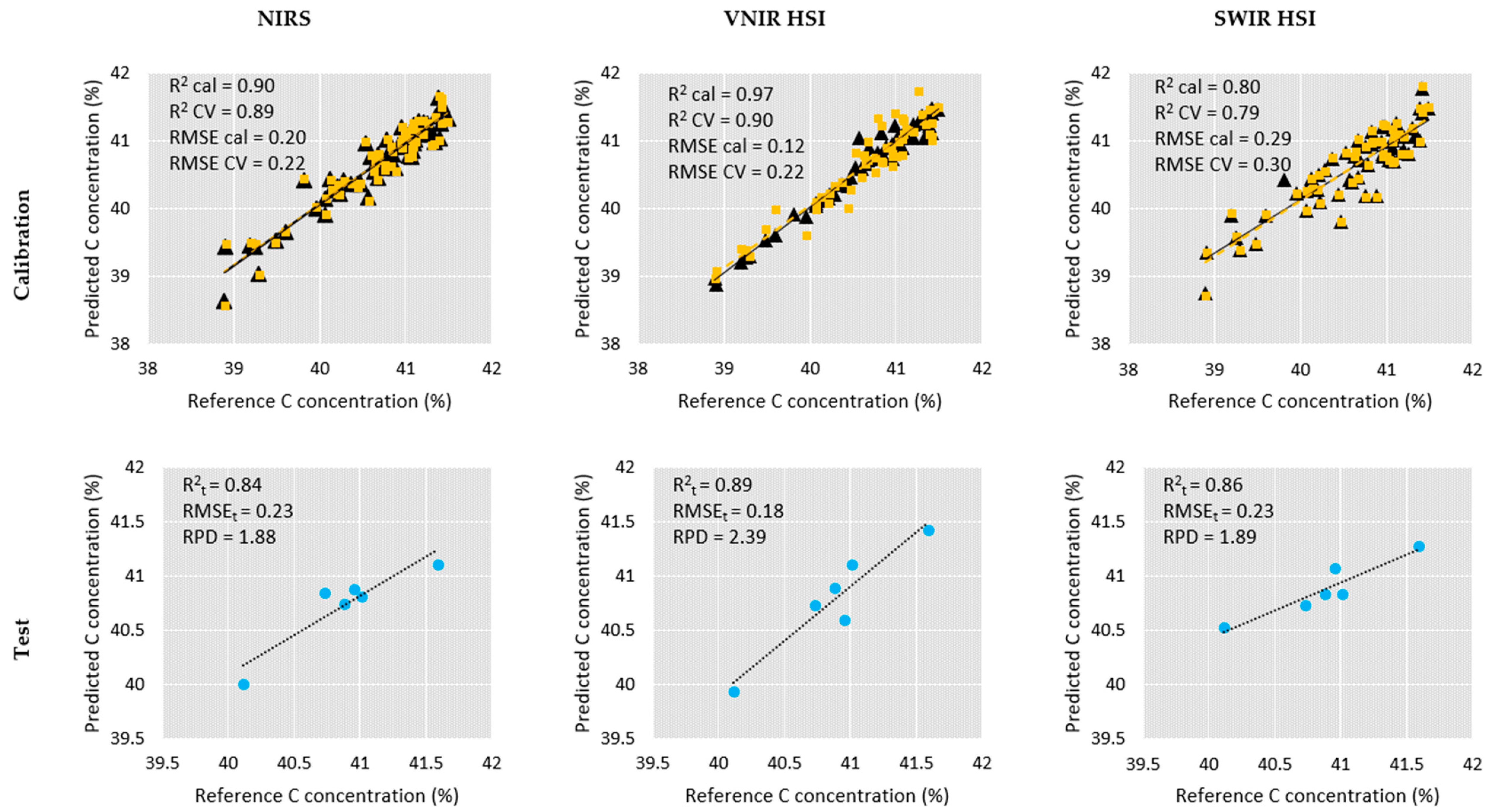
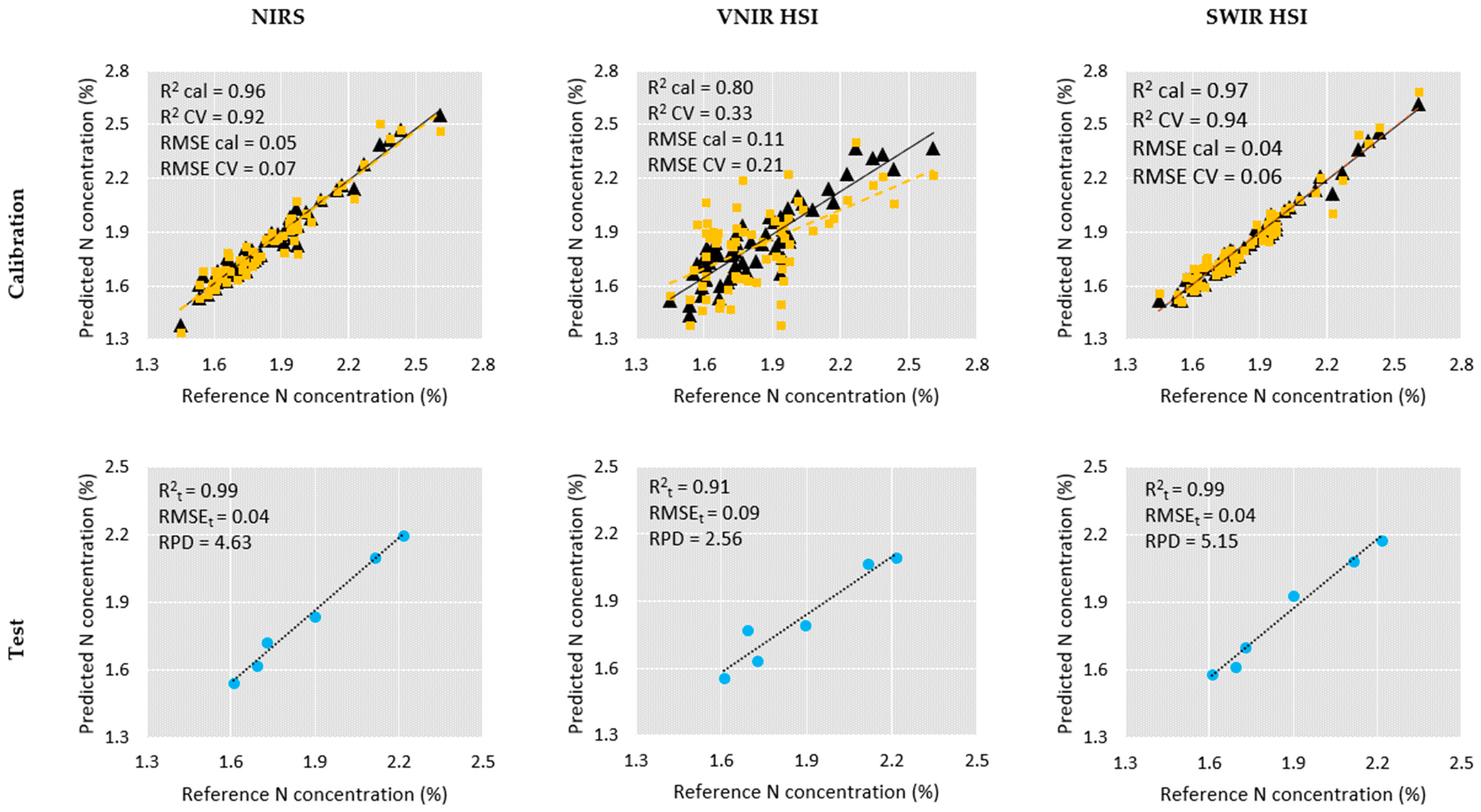
3.3. Attributes of the Models and Comparing Prediction Accuracies of PLSR Models
3.4. Important Spectral Regions for Predicting C and N Using Hyperspectral Cameras
4. Discussion
4.1. Technical
4.2. Application
5. Conclusions
Supplementary Materials
Author Contributions
Funding
Institutional Review Board Statement
Informed Consent Statement
Data Availability Statement
Acknowledgments
Conflicts of Interest
References
- Wilkinson, S. Big Data for Poultry–What Is Possible? In Proceedings of the 29th Annual Australian Poultry Science Symposium, Sydney, Australia, 4–7 February 2018; p. 152. Available online: https://poultry-research.sydney.edu.au/publications/.
- Moss, A.F.; Chrystal, P.V.; Cadogan, D.J.; Wilkinson, S.J.; Crowley, T.M.; Choct, M. Precision feeding and precision nutrition: A paradigm shift in broiler feed formulation? Anim. Biosci. 2021, 34, 354–362. [Google Scholar] [CrossRef]
- ACMF. Australian Industry Facts & Figures. Available online: https://www.chicken.org.au/facts-and-figures/ (accessed on 10 February 2020).
- Manley, M. Near-infrared spectroscopy and hyperspectral imaging: Non-destructive analysis of biological materials. Chem. Soc. Rev. 2014, 43, 8200–8214. [Google Scholar] [CrossRef] [Green Version]
- Kleyn, R. Chicken Nutrition: A Guide for Nutritionists and Poultry Professionals; Context: Leicestershire, UK, 2013. [Google Scholar]
- Moss, A.; Crowley, T.; Choct, M. Compilation and Assessment of the Variability of Nutrient Specifications for Commonly Used Australian Feed Ingredients. Proceedings the Australian Poultry Science Symposium, Sydney, Australia,, 16–19 February 2020. [Google Scholar]
- Tahmasbian, I.; Wallace, H.M.; Gama, T.; Hosseini Bai, S. An automated non-destructive prediction of peroxide value and free fatty acid level in mixed nut samples. LWT 2021, 143, 110893. [Google Scholar] [CrossRef]
- Khamsopha, D.; Woranitta, S.; Teerachaichayut, S. Utilizing near infrared hyperspectral imaging for quantitatively predicting adulteration in tapioca starch. Food Control 2021, 123, 107781. [Google Scholar] [CrossRef]
- Hu, N.; Li, W.; Du, C.; Zhang, Z.; Gao, Y.; Sun, Z.; Yang, L.; Yu, K.; Zhang, Y.; Wang, Z. Predicting micronutrients of wheat using hyperspectral imaging. Food Chem. 2021, 343, 128473. [Google Scholar] [CrossRef] [PubMed]
- Han, Y.; Liu, Z.; Khoshelham, K.; Bai, S.H. Quality estimation of nuts using deep learning classification of hyperspectral imagery. Comput. Electron. Agric. 2021, 180, 105868. [Google Scholar] [CrossRef]
- Sun, D.-W. Hyperspectral Imaging for Food Quality Analysis and Control; Elsevier: Amsterdam, The Netherlands, 2010. [Google Scholar]
- Elmasry, G.; Kamruzzaman, M.; Sun, D.-W.; Allen, P. Principles and applications of hyperspectral imaging in quality evaluation of agro-food products: A review. Crit. Rev. Food Sci. Nutr. 2012, 52, 999–1023. [Google Scholar] [CrossRef]
- Adão, T.; Hruška, J.; Pádua, L.; Bessa, J.; Peres, E.; Morais, R.; Sousa, J. Hyperspectral Imaging: A Review on UAV-Based Sensors, Data Processing and Applications for Agriculture and Forestry. Remote Sens. 2017, 9, 1110. [Google Scholar] [CrossRef] [Green Version]
- Eady, M.; Setia, G.; Park, B. Detection of Salmonella from chicken rinsate with visible/near-infrared hyperspectral microscope imaging compared against RT-PCR. Talanta 2019, 195, 313–319. [Google Scholar] [CrossRef]
- Lawrence, K.; Park, B.; Windham, W.; Mao, C. Calibration of a pushbroom hyperspectral imaging system for agricultural inspection. Trans. ASAE 2003, 46, 513. [Google Scholar] [CrossRef]
- Casada, M.; OBrien, K. Accuracy and repeatability of protein content measurements for wheat during storage. Appl. Eng. Agric. 2003, 19, 203. [Google Scholar] [CrossRef] [Green Version]
- Tahmasbian, I.; Hosseini Bai, S.; Wang, Y.; Boyd, S.; Zhou, J.; Esmaeilani, R.; Xu, Z. Using laboratory-based hyperspectral imaging method to determine carbon functional group distributions in decomposing forest litterfall. Catena 2018, 167, 18–27. [Google Scholar] [CrossRef]
- Bai, S.H.; Tahmasbian, I.; Zhou, J.; Nevenimo, T.; Hannet, G.; Walton, D.; Randall, B.; Gama, T.; Wallace, H.M. A non-destructive determination of peroxide values, total nitrogen and mineral nutrients in an edible tree nut using hyperspectral imaging. Comput. Electron. Agric. 2018, 151, 492–500. [Google Scholar] [CrossRef]
- Da Conceição, R.R.P.; Simeone, M.L.F.; Queiroz, V.A.V.; De Medeiros, E.P.; De Araújo, J.B.; Coutinho, W.M.; Da Silva, D.D.; De Araújo Miguel, R.; De Paula Lana, U.G.; De Resende Stoianoff, M.A. Application of near-infrared hyperspectral (NIR) images combined with multivariate image analysis in the differentiation of two mycotoxicogenic Fusarium species associated with maize. Food Chem. 2021, 344, 128615. [Google Scholar] [CrossRef] [PubMed]
- Fu, Y.; Yang, G.; Song, X.; Li, Z.; Xu, X.; Feng, H.; Zhao, C. Improved Estimation of Winter Wheat Aboveground Biomass Using Multiscale Textures Extracted from UAV-Based Digital Images and Hyperspectral Feature Analysis. Remote Sens. 2021, 13, 581. [Google Scholar] [CrossRef]
- Xu, X.; Fan, L.; Li, Z.; Meng, Y.; Feng, H.; Yang, H.; Xu, B. Estimating Leaf Nitrogen Content in Corn Based on Information Fusion of Multiple-Sensor Imagery from UAV. Remote Sens. 2021, 13, 340. [Google Scholar] [CrossRef]
- Wold, S.; Sjöström, M.; Eriksson, L. PLS-regression: A basic tool of chemometrics. Chemom. Intellig. Lab. Syst. 2001, 58, 109–130. [Google Scholar] [CrossRef]
- Wold, S.; Ruhe, A.; Wold, H.; Dunn, I.; Dunn, W.J. The collinearity problem in linear regression. The partial least squares (PLS) approach to generalized inverses. SIAM J. Sci. Stat. Comput. 1984, 5, 735–743. [Google Scholar] [CrossRef] [Green Version]
- Höskuldsson, A. PLS regression methods. J. Chemom. 1988, 2, 211–228. [Google Scholar] [CrossRef]
- Tahmasbian, I.; Xu, Z.; Abdullah, K.; Zhou, J.; Esmaeilani, R.; Nguyen, T.T.N.; Hosseini Bai, S. The potential of hyperspectral images and partial least square regression for predicting total carbon, total nitrogen and their isotope composition in forest litterfall samples. J. Soils Sed. 2017, 17, 2091–2103. [Google Scholar] [CrossRef]
- Barbin, D.F.; ElMasry, G.; Sun, D.-W.; Allen, P. Predicting quality and sensory attributes of pork using near-infrared hyperspectral imaging. Anal. Chim. Acta 2012, 719, 30–42. [Google Scholar] [CrossRef] [PubMed]
- Kämper, W.; Trueman, S.J.; Tahmasbian, I.; Bai, S.H. Rapid Determination of Nutrient Concentrations in Hass Avocado Fruit by Vis/NIR Hyperspectral Imaging of Flesh or Skin. Remote Sens. 2020, 12, 3409. [Google Scholar] [CrossRef]
- Malmir, M.; Tahmasbian, I.; Xu, Z.; Farrar, M.B.; Bai, S.H. Prediction of macronutrients in plant leaves using chemometric analysis and wavelength selection. J. Soils Sed. 2020, 20, 249–259. [Google Scholar] [CrossRef]
- Kohavi, R. A study of cross-validation and bootstrap for accuracy estimation and model selection. In Proceedings of the International Joint Conference on Artificial Intelligence (Ijcai), Montreal, QC, Canada, 20–25 August 1995; pp. 1137–1145. [Google Scholar]
- Malmir, M.; Tahmasbian, I.; Xu, Z.; Farrar, M.B.; Bai, S.H. Prediction of soil macro- and micro-elements in sieved and ground air-dried soils using laboratory-based hyperspectral imaging technique. Geoderma 2019, 340, 70–80. [Google Scholar] [CrossRef]
- Shen, L.; Gao, M.; Yan, J.; Li, Z.-L.; Leng, P.; Yang, Q.; Duan, S.-B. Hyperspectral Estimation of Soil Organic Matter Content using Different Spectral Preprocessing Techniques and PLSR Method. Remote Sens. 2020, 12, 1206. [Google Scholar] [CrossRef] [Green Version]
- Bellon-Maurel, V.; Fernandez-Ahumada, E.; Palagos, B.; Roger, J.-M.; McBratney, A. Critical review of chemometric indicators commonly used for assessing the quality of the prediction of soil attributes by NIR spectroscopy. Trends Anal. Chem. 2010, 29, 1073–1081. [Google Scholar] [CrossRef]
- Sillero, A.M.; Pierna, J.A.F.; Sinnaeve, G.; Dardenne, P.; Baeten, V. Quantification of protein in wheat using near infrared hyperspectral imaging: Performance comparison with conventional near infrared spectroscopy. J. Near Infrared Spectrosc. 2018. [Google Scholar] [CrossRef]
- Fu, Y.; Yang, G.; Pu, R.; Li, Z.; Li, H.; Xu, X.; Song, X.; Yang, X.; Zhao, C. An overview of crop nitrogen status assessment using hyperspectral remote sensing: Current status and perspectives. Eur. J. Agron. 2021, 124, 126241. [Google Scholar] [CrossRef]
- Chew, L.; Prasad, K.N.; Amin, I.; Azrina, A.; Lau, C. Nutritional composition and antioxidant properties of Canarium odontophyllum Miq.(dabai) fruits. J. Food Compos. Anal. 2011, 24, 670–677. [Google Scholar] [CrossRef]
- Bai, S.H.; Darby, I.; Nevenimo, T.; Hannet, G.; Hannet, D.; Poienou, M.; Grant, E.; Brooks, P.; Walton, D.; Randall, B.J.P.o. Effects of roasting on kernel peroxide value, free fatty acid, fatty acid composition and crude protein content. PLoS ONE 2017, 12, e0184279. [Google Scholar]
- Burger, J.; Geladi, P. Hyperspectral NIR imaging for calibration and prediction: A comparison between image and spectrometer data for studying organic and biological samples. Analyst 2006, 131, 1152–1160. [Google Scholar] [CrossRef]
- Nawar, S.; Mouazen, A.M. Optimal sample selection for measurement of soil organic carbon using on-line vis-NIR spectroscopy. Comput. Electron. Agric. 2018, 151, 469–477. [Google Scholar] [CrossRef]
- Viscarra Rossel, R.A.; Walvoort, D.J.J.; McBratney, A.B.; Janik, L.J.; Skjemstad, J.O. Visible, near infrared, mid infrared or combined diffuse reflectance spectroscopy for simultaneous assessment of various soil properties. Geoderma 2006, 131, 59–75. [Google Scholar] [CrossRef]
- Cozzolino, D.; Morón, A. Potential of near-infrared reflectance spectroscopy and chemometrics to predict soil organic carbon fractions. Soil Tillage Res. 2006, 85, 78–85. [Google Scholar] [CrossRef]
- Tahmasbian, I.; Xu, Z.; Boyd, S.; Zhou, J.; Esmaeilani, R.; Che, R.; Bai, S.H. Laboratory-based hyperspectral image analysis for predicting soil carbon, nitrogen and their isotopic compositions. Geoderma 2018, 330, 254–263. [Google Scholar] [CrossRef]
- Curran, P.J. Remote sensing of foliar chemistry. Remote Sens. Environ. 1989, 30, 271–278. [Google Scholar] [CrossRef]
- Datt, B. Remote Sensing of Chlorophyll a, Chlorophyll b, Chlorophyll a+b, and Total Carotenoid Content in Eucalyptus Leaves. Remote Sens. Environ. 1998, 66, 111–121. [Google Scholar] [CrossRef]
- Sun, D.-W. Infrared Spectroscopy for Food Quality Analysis and Control; Academic Press: Burlington, MA, USA, 2009. [Google Scholar]
- Salgó, A.; Gergely, S. Analysis of wheat grain development using NIR spectroscopy. J. Cereal Sci. 2012, 56, 31–38. [Google Scholar] [CrossRef]
- Zhou, P.; Zhang, Y.; Yang, W.; Li, M.; Liu, Z.; Liu, X. Development and performance test of an in-situ soil total nitrogen-soil moisture detector based on near-infrared spectroscopy. Comput. Electron. Agric. 2019, 160, 51–58. [Google Scholar] [CrossRef]
- Moss, A.; Chrystal, P.; Crowley, T.; Pesti, G. Raw material nutrient variability has substantial impact on the potential profitability of chicken meat production. J. Appl. Poult. Res. 2021, 30, 100129. [Google Scholar] [CrossRef]
- Nahm, K. Feed formulations to reduce N excretion and ammonia emission from poultry manure. Bioresour. Technol. 2007, 98, 2282–2300. [Google Scholar] [CrossRef] [PubMed]
- Ritz, C.; Fairchild, B.; Lacy, M. Implications of ammonia production and emissions from commercial poultry facilities: A review. J. Appl. Poult. Res. 2004, 13, 684–692. [Google Scholar] [CrossRef]
- Moss, A.; Parkinson, G.; Crowley, T.; Pesti, G. Alternatives to formulate laying hen diets beyond the traditional least-cost model. J. Appl. Poult. Res. 2021, 30, 100137. [Google Scholar] [CrossRef]


| Calibration (63 Samples) | Test (6 Samples) | |||
|---|---|---|---|---|
| C (%) | N (%) | C (%) | N (%) | |
| Mean | 40.64 | 1.84 | 40.88 | 1.88 |
| Min | 38.89 | 1.45 | 40.11 | 1.61 |
| Max | 41.49 | 2.61 | 41.59 | 2.22 |
| Range | 2.60 | 1.16 | 1.48 | 0.61 |
| SD | 0.65 | 0.24 | 0.48 | 0.25 |
| Coefficient of variations | 1.61 | 13.16 | 1.17 | 13.07 |
| WL (nm) | LV | TF | R2 cal | R2 CV | RMSE cal (%) | RMSE CV (%) | Test R2 | Test RMSE | RPD | |
|---|---|---|---|---|---|---|---|---|---|---|
| NIRS | 400–2500 | 4 | - | 0.90 | 0.89 | 0.20 | 0.22 | 0.84 | 0.23 | 1.88 |
| VNIR camera | 400–1000 | 7 | OSC | 0.97 | 0.90 | 0.12 | 0.22 | 0.89 | 0.18 | 2.39 |
| SWIR camera | 1000–2515 | 7 | OSC, DT | 0.80 | 0.80 | 0.29 | 0.30 | 0.86 | 0.23 | 1.89 |
| VNIR camera | 400–550 | 5 | OSC | 0.93 | 0.78 | 0.17 | 0.31 | 0.86 | 0.21 | 2.03 |
| 551–700 | 8 | - | 0.50 | 0.16 | 0.45 | 0.57 | 0.56 | 0.31 | 1.39 | |
| 701–850 | 4 | - | 0.26 | 0.08 | 0.55 | 0.62 | 0.40 | 0.34 | 1.30 | |
| 851–1000 | 5 | - | 0.64 | 0.48 | 0.38 | 0.47 | 0.45 | 0.39 | 1.13 | |
| SWIR camera | 1000–1150 | 1 | OSC | 0.68 | 0.68 | 0.37 | 0.38 | 0.46 | 0.40 | 1.09 |
| 1151–1300 | 7 | - | 0.60 | 0.34 | 0.41 | 0.53 | 0.41 | 0.47 | 0.92 | |
| 1301–1450 | 1 | OSC | 0.69 | 0.69 | 0.36 | 0.37 | 0.29 | 0.43 | 1.01 | |
| 1451–1600 | 1 | OSC | 0.72 | 0.74 | 0.34 | 0.35 | 0.80 | 0.34 | 1.52 | |
| 1601–1750 | 6 | - | 0.63 | 0.43 | 0.39 | 0.51 | 0.40 | 0.42 | 1.04 | |
| 1751–1900 | 3 | - | 0.65 | 0.61 | 0.38 | 0.42 | 0.41 | 0.43 | 1.02 | |
| 1901–2050 | 2 | - | 0.66 | 0.62 | 0.38 | 0.40 | 0.33 | 0.45 | 0.97 | |
| 2051–2200 | 4 | - | 0.63 | 0.54 | 0.39 | 0.44 | 0.00 | 0.00 | 0.00 | |
| 2201–2350 | 5 | - | 0.55 | 0.28 | 0.43 | 0.56 | 0.41 | 0.48 | 0.91 | |
| 2351–2515 | 5 | - | 0.73 | 0.64 | 0.34 | 0.39 | 0.35 | 0.41 | 1.04 |
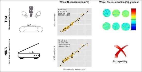
| WL (nm) | LV | TF | R2 cal | R2 CV | RMSE cal (%) | RMSE CV (%) | Test R2 | Test RMSE | RPD | |
|---|---|---|---|---|---|---|---|---|---|---|
| NIRS | 400–2500 | 10 | - | 0.96 | 0.92 | 0.05 | 0.07 | 0.99 | 0.05 | 4.63 |
| VNIR camera | 400–1000 | 13 | - | 0.80 | 0.33 | 0.11 | 0.21 | 0.91 | 0.09 | 2.56 |
| SWIR camera | 1000–2515 | 8 | - | 0.97 | 0.94 | 0.04 | 0.06 | 0.99 | 0.04 | 5.15 |
| VNIR camera | 400–550 | 1 | - | 0.0 | 0.0 | 0.0 | 0.0 | NC | NC | NC |
| 551–700 | 1 | - | 0.0 | 0.0 | 0.0 | 0.0 | NC | NC | NC | |
| 701–850 | 2 | - | 0.1 | 0.06 | 0.23 | 0.24 | NC | NC | NC | |
| 851–1000 | 6 | OSC | 0.68 | 0.71 | 0.09 | 0.13 | 0.30 | 0.19 | 1.18 | |
| SWIR camera | 1000–1150 | 8 | - | 0.82 | 0.70 | 0.10 | 0.13 | 0.93 | 0.06 | 3.14 |
| 1151–1300 | 8 | - | 0.93 | 0.88 | 0.06 | 0.08 | 0.93 | 0.11 | 2.07 | |
| 1301–1450 | 6 | - | 0.55 | 0.39 | 0.16 | 0.19 | 0.95 | 0.07 | 3.08 | |
| 1451–1600 | 6 | - | 0.91 | 0.89 | 0.07 | 0.08 | 0.99 | 0.06 | 3.80 | |
| 1601–1750 | 6 | - | 0.92 | 0.85 | 0.07 | 0.09 | 0.83 | 0.11 | 2.11 | |
| 1751–1900 | 7 | - | 0.87 | 0.78 | 0.08 | 0.12 | 0.88 | 0.10 | 2.33 | |
| 1901–2050 | 6 | - | 0.92 | 0.89 | 0.07 | 0.08 | 0.96 | 0.06 | 3.47 | |
| 2051–2200 | 5 | - | 0.92 | 0.87 | 0.06 | 0.07 | 0.95 | 0.06 | 3.52 | |
| 2201–2350 | 6 | - | 0.81 | 0.72 | 0.10 | 0.13 | 0.71 | 0.13 | 1.70 | |
| 2351–2515 | 3 | - | 0.36 | 0.30 | 0.19 | 0.20 | 0.21 | 0.21 | 1.06 |
Publisher’s Note: MDPI stays neutral with regard to jurisdictional claims in published maps and institutional affiliations. |
© 2021 by the authors. Licensee MDPI, Basel, Switzerland. This article is an open access article distributed under the terms and conditions of the Creative Commons Attribution (CC BY) license (http://creativecommons.org/licenses/by/4.0/).
Share and Cite
Tahmasbian, I.; Morgan, N.K.; Hosseini Bai, S.; Dunlop, M.W.; Moss, A.F. Comparison of Hyperspectral Imaging and Near-Infrared Spectroscopy to Determine Nitrogen and Carbon Concentrations in Wheat. Remote Sens. 2021, 13, 1128. https://0-doi-org.brum.beds.ac.uk/10.3390/rs13061128
Tahmasbian I, Morgan NK, Hosseini Bai S, Dunlop MW, Moss AF. Comparison of Hyperspectral Imaging and Near-Infrared Spectroscopy to Determine Nitrogen and Carbon Concentrations in Wheat. Remote Sensing. 2021; 13(6):1128. https://0-doi-org.brum.beds.ac.uk/10.3390/rs13061128
Chicago/Turabian StyleTahmasbian, Iman, Natalie K. Morgan, Shahla Hosseini Bai, Mark W. Dunlop, and Amy F. Moss. 2021. "Comparison of Hyperspectral Imaging and Near-Infrared Spectroscopy to Determine Nitrogen and Carbon Concentrations in Wheat" Remote Sensing 13, no. 6: 1128. https://0-doi-org.brum.beds.ac.uk/10.3390/rs13061128