Article

Influencing Factors in Estimation of Leaf Angle Distribution of an Individual Tree from Terrestrial Laser Scanning Data

1
State Key Laboratory of Remote Sensing Science, Faculty of Geographical Science, Beijing Normal University, Beijing 100875, China
2
College of Resources and Environment, University of Chinese Academy of Sciences, Beijing 100049, China
3
Key Laboratory for Silviculture and Conservation of Ministry of Education, Beijing Forestry University, Beijing 100083, China
*
Author to whom correspondence should be addressed.
Submission received: 25 January 2021 / Revised: 15 March 2021 / Accepted: 16 March 2021 / Published: 18 March 2021
(This article belongs to the Special Issue Leaf and Canopy Biochemical and Biophysical Variables Retrieval)

Abstract

:
Leaf angle distribution (LAD) is an important attribute of forest canopy architecture and affects the solar radiation regime within the canopy. Terrestrial laser scanning (TLS) has been increasingly used in LAD estimation. The point clouds data suffer from the occlusion effect, which leads to incomplete scanning and depends on measurement strategies such as the number of scans and scanner location. Evaluating these factors is important to understand how to improve LAD, which is still lacking. Here, we introduce an easy way of estimating the LAD using open source software. Importantly, the influence of the occlusion effect on the LAD was evaluated by combining the proposed complete point clouds (CPCs) with the simulated data of 3D tree models of Aspen, Pin Oak and White Oak. We analyzed the effects of the point density, the number of scans and the scanner height on the LAD and G-function. Results show that: (1) the CPC can be used to evaluate the TLS-based normal vector reconstruction accuracy without an occlusion effect; (2) the accuracy is slightly affected by the normal vector reconstruction method and is greatly affected by the point density and the occlusion effect. The higher the point density (with a number of points per unit leaf area of 0.2 cm−2 to 27 cm−2 tested), the better the result is; (3) the performance is more sensitive to the scanner location than the number of scans. Increasing the scanner height improves LAD estimation, which has not been seriously considered in previous studies. It is worth noting that relatively tall trees suffer from a more severe occlusion effect, which deserves further attention in further study.

1. Introduction

The leaf angle distribution (LAD) is a mathematical description of the orientation of leaves [1]; it determines the radiation transmission within vegetation canopies [2] and has a direct impact on the estimation of other important structural parameters: fraction of absorbed photosynthetically active radiation (FPAR) [3,4] and leaf area index (LAI) [5,6,7]. The LAD determines the leaf projection coefficient (the G-function), which is usually assumed to be 0.5 due to the difficulty in an accurate and efficient measurement. However, such an assumption may cause significant errors in Beer’s law-based LAI retrieval [8,9] when the actual LAD deviates from the spherical distribution.
The leaf orientation can be described by two separate angles for an individual leaf: the inclination angle and the azimuth angle [10]. The leaf inclination angle denotes the angle between the plane or axis of a leaf lamina and the horizontal plane [11], and the azimuth angle denotes the azimuth direction of the vector normal to the leaf’s upper surface [10]. A uniform azimuth direction is usually assumed for most species [9,12,13]; thus, the azimuth angle is not within the scope of this paper and the leaf inclination angle distribution is used to describe the LAD. The LAD function defines the probability of leaf normal falling within a unit interval of inclination angle [9] for a tree or the whole canopy.
Several LAD functions [12] have been proposed to define the nonrandom distribution of the leaf inclination angle with one [8,14,15] or two parameters [13,16]. Typical forms include trigonometric distribution [8], two-parameter beta distribution [13], ellipsoidal distribution [14], elliptical distribution [16], and rotated ellipsoidal distribution functions [15]. Ross [9] summarized six typical LADs: spherical, uniform, planophile, erectophile, plagiophile, and extremophile distributions. These mathematical models are approximate descriptions of the LAD; in general, a spherical distribution is adopted because the corresponding G-function is always 0.5 in any viewing zenith angle and is also approximately 0.5 for other typical LADs when the viewing zenith angle is close to 57.3° [1]; thus, no measurement of the LAD is needed. However, considerable deviations were found for other viewing angles when replacing the actual LAD with the spherical distribution assumption (G = 0.5). For the whole hemisphere, the G value may vary from 0.27 to 0.84 for six typical LADs listed by De Wit [8]. The general viewing zenith angles of terrestrial laser scanning (TLS) are far from 57.3°, and the assumption of 0.5 for the G value may introduce large errors in LAI retrieval. As a result, it is necessary to obtain the real LAD and G-function in TLS measurements.
TLS, which swings a tiny footprint laser and provides accurate measurement of distances to objects, is a promising tool for measuring leaf angles [7,17,18,19,20]. By using a large number of sampling laser beams within the instrument field of view (FOV), TLS can generate point clouds positioned in three-dimensional (3D) space [7]. Related methods can be divided into five categories: inversion, leaf plane fitting, the voxel-based method, normal vector reconstruction of adjacent points, and triangulation. (i) The inversion method: Zhao et al. [21] proposed a method that inverts the leaf angle information using maximum likelihood estimation, which is based on the probability that the laser pulses and the vegetation intersect. It is a physical–statistical approach and depends on model and parameters selection. (ii) The leaf plane fitting method: manually extracting complete leaves [7,22] or automatically segmenting leaf clusters [23,24]. As a semiautomatic method, plane fitting of the artificially clipped point clouds of complete leaves from the tree was performed to calculate the normal vectors [7,22]; the leaf inclination angle is computed from the angle of the normal vector with respect to the zenith. Furthermore, some studies proposed automatic leaf segmentation algorithms based on the Gaussian mixture model [24] or k-Means [23] to estimate LAD from the leaf clusters. (iii) The voxel-based method: instead of extracting leaf clusters, a plane was fitted to some voxels with a size of 5 mm surrounding the point (voxel) of interest in [25]. (iv) Normal vector reconstruction of adjacent points: adjacent points of a fixed number [17,20] or within a sphere of a given radius [26,27] were used. Zheng and Moskal [17] proposed a least squares fitting technique to reconstruct the normal vector for a specific point according to its six adjacent points, and the inclination of the plane where the central point is located can be calculated from the normal vector. A possible source of error is that adjacent points may not be on the same leaf. Vicari et al. [20] developed an improved method by introducing a threshold based on the covariance matrix of neighborhood points, and points with large errors were eliminated from the LAD statistic. In methods of obtaining adjacent points through a spherical search, the radius of the neighborhood distance was constrained by the leaf size in [26] to avoid adjacent points on different leaves; a radius of 2.5 cm was used in [27], and the number of hits was corrected for LAD statistic, given that it depends on the leaf orientation relative to the view direction of the laser. (v) The triangulation method: Bailey and Mahaffee [18] developed a rapid LAD estimation method based on the triangulation of point clouds: the normal vector of the plane formed by three adjacent points is directly calculated. This method is relatively simple to implement but could be sensitive to noise and the positioning error of the TLS system. Many researchers have proposed practical TLS-based LAD estimation methods, but their implementation usually requires additional programming. The commonly used point clouds processing software CloudCompare (http://cloudcompare.org) (accessed on 16 March 2021), an open source project, has a function for directly calculating the normal vector of each point, making the calculation of the leaf inclination angle more feasible. Thus, we intend to use this function to estimate the LAD in our TLS-based LAD measurements.
In addition to the estimation method, the point clouds data themselves are also a major factor affecting the LAD estimation accuracy. The accuracy values calculated from point clouds with different point densities or point clouds acquired from different scanning strategies, e.g., the number of scans and scan locations are different. Vicari et al. [20] demonstrated that the point density is a major constraining factor in the accuracy of LAD estimation and suggested the use of multiple scans to improve the accuracy. However, another study showed that there is a limited effect of point density sampling on the foliage element orientation when the nearest point distance is less than 2 cm [19]. The analysis was performed using field-measured TLS data of an artificial tree, where the absolute true LAD is unknown. Therefore, the influence of the point density on the LAD measurement still requires further investigation. Moreover, the number and locations of TLS scans are also important factors affecting the quality of the point clouds [28]; however, the analysis of their impacts on the LAD are less studied. In practical LAD measurements of individual trees, three [17], four [18,20], five [19], or six [24] scanning locations have been used. In terms of scanning location, a scanner height of 1.5 m, which is the general height of a TLS tripod [29], was usually adopted [20,22,25]. It should be noted that point clouds data are affected by the occlusion effect—“laser pulses are blocked – at least partially – by leaves, keeping the pulses from making contact with leaves located further along their path”, as defined by Béland et al. [29]. The occlusion effect is directly relevant to the observation geometry, and thus varies across scanning strategies. However, the influence of occlusion on the estimation accuracy of the LAD is rarely analyzed because of the difficulty in the validation process.
In validation, early methods generally used manual measurements. However, Bailey and Mahaffee [18] found that manual measurements contain substantial errors that seriously depend on the individuals performing the measurements. Thus, the true leaf inclination angle is difficult to obtain, and manually measured angles are not necessarily more accurate than those obtained from TLS. With the development of computer simulation models [30], such as librat [31], Heidelberg LiDAR Operations Simulator (HELIOS) [32] and Discrete Anisotropic Radiative Transfer (DART) [33,34], both the simulated TLS point clouds and the true LAD are available [20]. Therefore, we intend to use the computer simulation, which has been adopted in previous LAD studies [18,20], to evaluate the accuracy of the method. Note that even though computer simulation techniques can be used to avoid the problem of lacking the true LAD in evaluating LAD estimation methods, occlusion effects exist in simulated data as well because not all leaves can be scanned. Occlusion has been identified as a major source of uncertainty in the estimation of vegetation structure parameters [35,36,37,38,39] and has been considered as a source of error in LAD estimation using TLS [19,20,22]; however, current methods for investigating its influence are lacking. As it is hard to evaluate with just field-measured or simulated TLS data, we developed an approach for analyzing the influence of the occlusion effect by introducing complete point clouds (CPC), which is obtained through mathematical calculation and does not suffer from occlusion.
Based on the simulated point clouds data and the CPC, we investigate the effect of several influencing factors in TLS measurements on the calculation of LAD and G-function, which are important input parameters in radiative transfer modelling [40] and indirect LAI measurement. The studied influencing factors include the point density, the number of scans, the scanner height, and the occlusion effect. A better understanding of these effects is significant not only in future improvement of LAD estimation, but also in measurement setup optimization when estimating other forest structural parameters from TLS.

2. Materials and Methods

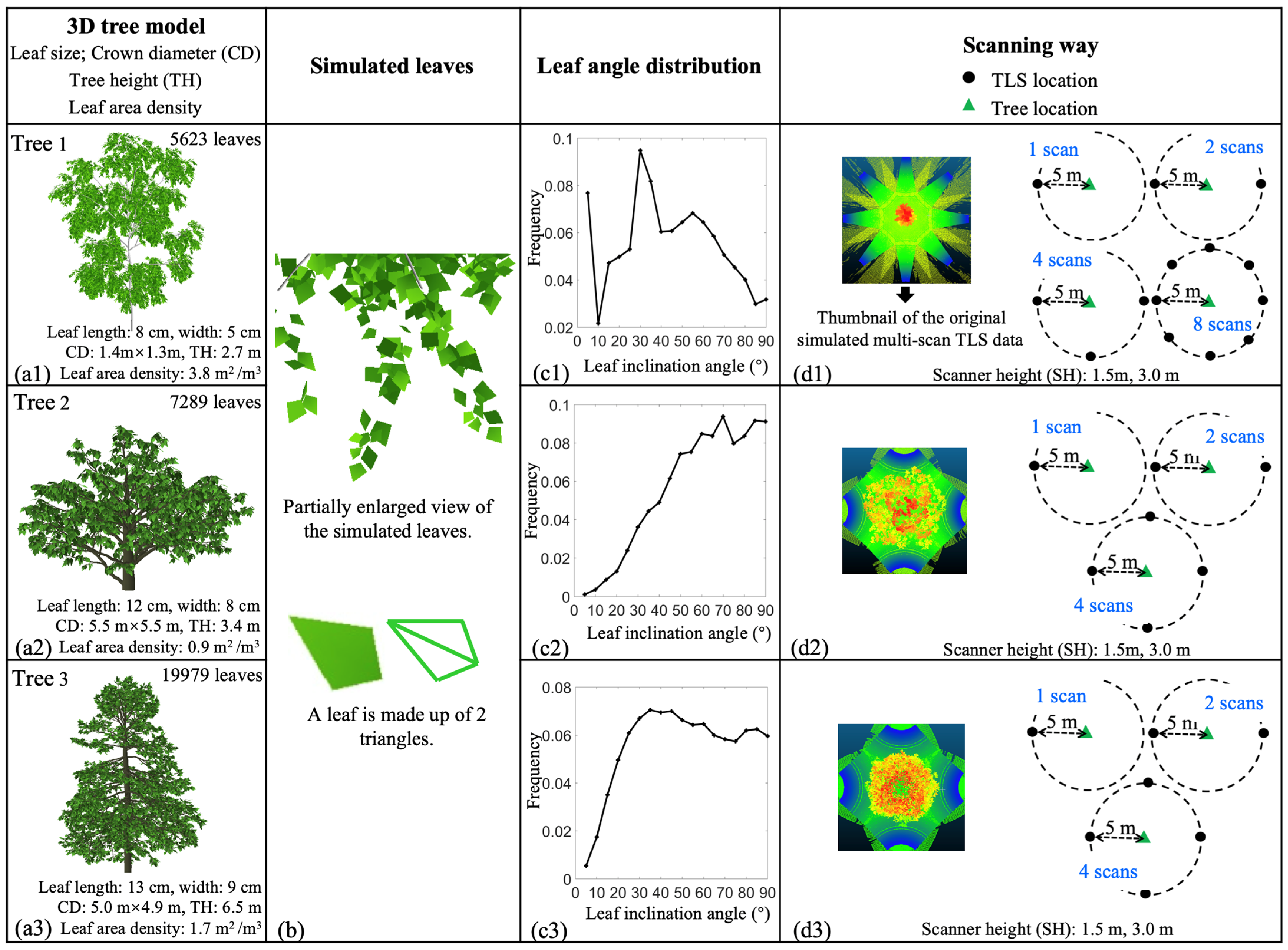
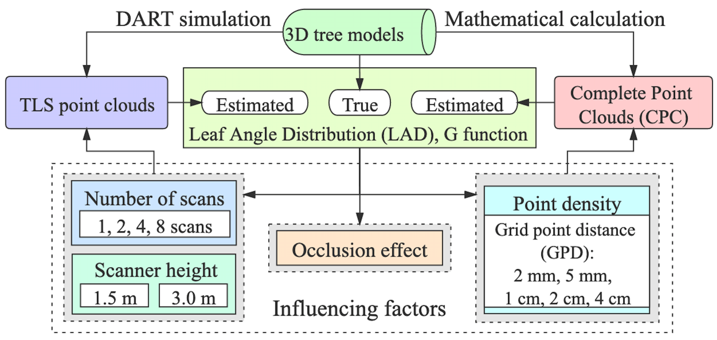
2.1. Simulated Point Clouds Data

Three tree models of different species (Tree1—Aspen, Tree2—Pin Oak, and Tree3—White Oak) were generated in OnyxTREE (http://www.onyxtree.com/) (accessed on 16 March 2021); each of the leaves were made up of two triangles. Average leaf sizes for each tree were different, with an average leaf length and width—8 cm × 5 cm, 12 cm × 8 cm, and 13 cm   × 9 cm for Tree1, Tree2, and Tree3, respectively. The leaf area density (defined as the one-sided leaf area per volumetric unit (m3) [7]), is calculated from the ratio of the total leaf area and the crown volume, and the crown volume is the volume of the envelope reconstructed from the simulated point clouds. There were large differences between the three tree models. The crown diameter (CD) (east–west) and tree height (TH) were very small for Tree1 (Aspen) (1.4 m × 1.3 m and 2.7 m, respectively), but the leaf area density (3.8 m2/m3) was the largest of all three trees (Figure 1(a1)). The CD of Tree2 (Pin Oak) (5.5 m × 5.5 m) was much larger than that of Tree1, and the TH (3.4 m) was slightly taller than that of Tree1 (Figure 1(a2)), with a leaf area density of 0.9 m2/m3. Tree3 (White Oak) was the tallest of all of three trees (6.5 m), and the CD was similar with that of Tree2, with a leaf area density of 1.7 m2/m3 (Figure 1(a3)). The true LAD of each tree (illustrated in Figure 1(c1–c3), respectively) was calculated based on the coordinates of the triangles.
Simulated TLS point clouds were generated for the three 3D tree models based on the DART model, which can simulate the Light Detection and Ranging (LiDAR) data based on a quasi-Monte Carlo ray tracing approach [34]. The parameter settings in the DART simulation were the same as those in FARO Focus 3D X330 TLS [41]. The wavelength of the laser beam was 1550 nm, the beam divergence was 0.19 mrad (corresponding to an increase in spot size of 0.95 mm at a distance of 5 m), and the beam waist diameter (1/e) was 2.25 mm. The scanner heights (SHs) were 1.5 m and 3 m. Additionally, branches were excluded in the DART simulations to avoid the influence of woody materials on the LAD. DART TLS simulations were performed at eight locations around Tree1 (Figure 1(d1)) and four locations around Tree2 (Figure 1(d2)) and Tree3 (Figure 1(d3)). The distance between the scanner and the center of the tree was 5 m for each simulation; the scan angle resolution in both the zenith and azimuth direction was set to 0.05°, with an average distance between the center points of two neighboring laser spots being 4 mm at 5 m. In in-situ laser scanning, several target balls should be adequately positioned in the field before scanning; the point clouds acquired from different scans are registered into the same coordinate system based on these common targets. Different from the field measurement, registration of different scans is not needed. Data from multi-location scanning can be directly merged together (using “Merge” function in CloudCompare) because the simulations were performed in the same coordinate system, thus there is no registration error.
A point thinning procedure was performed to reduce redundant points. To investigate the influencing factors (shown in Figure 2), comparison between LADs computed from single-scan and multi-scan data, and each of them with the LADs computed from the complete point clouds (CPC) with equal point density on each leaf (see Section 2.4), are needed. Regions that can be scanned from two or more locations are oversampled, resulting in larger point density than those that are just scanned once, if we merge multi-scan data directly. Considering that the point density affects the LAD estimation, the merged point clouds were thinned using the “subsample” function in CloudCompare 2.10.1 by setting the minimum space between points (we call it the least neighbor point distance (NPD)) to 5 mm to reduce redundant points. Selecting points from the original point clouds, no point in the output data is closer to another point than the specified NPD after the subsample. This makes the point densities at different regions of the tree more consistent than the original data. In addition, the point thinning process was also applied to the single-scan TLS data to obtain an NPD of 5 mm, making it comparable in point density to the merged multi-scan point clouds.

2.2. LAD Estimation

An automatic method was used to reconstruct the normal vectors of all points of a tree; the basic principle is to extract the nearest neighbor points around each point through a spherical search with a certain radius, and then perform the plane fitting. A referenced radius can be obtained from the normal computation in CloudCompare 2.10.1. After several tests, we found that the radius automatically calculated by the software was usually close to four times the NPD; thus, this value was used as the searching radius, and the accuracy of LAD estimation was tested. The normal vector n   is set to be oriented to the upper hemisphere and is calculated from the covariance matrix of the neighborhood points [17]. If we set the zenith vector to   z (0,0,1), the leaf inclination angle   a can be calculated as [20]:
a = cos 1 [ z · n z · n ] · 180 ° π
The probability density function of leaf inclination angle ( a ) at 5-degree intervals is calculated to obtain the LAD.

2.3. G-function Calculation

The G-function is the mean projection of the leaf area unit in a plane perpendicular to the sunrays [6]. The G value is a constant 0.5 for spherical distribution. For TLS measurements, the viewing direction is equivalent to the incident direction. Assuming the azimuth angle to be uniform, the G-function is computed as:
G ( θ ) = 0 π 2 A ( θ , θ l ) g ( θ l ) sin θ l d ( θ l )
A ( θ , θ l ) = { cos θ cos θ l ,     | cot θ cot θ l | > 1 cos θ cos θ l   [ 1 + ( 2 / π ) ( tan ψ ψ ) ] ,     | cot θ cot θ l | 1
where ψ = c o s 1 ( cot θ cot θ l ) θ is the viewing zenith angle, θ l is the leaf inclination angle, and g ( θ l ) is the probability density function that describes the leaf inclination distribution function, which can be obtained through the automatic normal vector calculation of point clouds data.

2.4. Validation

(1) Calculating the true LAD and G-function from the 3D tree model. The tree models are made up of triangles of which the coordinates of the vertexes are known. The true leaf inclination angle, LAD, and G-function can be calculated directly based on each definition.
(2) Generating simulated TLS point clouds to analogize actual measurement. The 3D tree models were input into the DART model, and the simulated TLS data were obtained. The simulated TLS data together with the known LAD allow us to perform a validation. We estimate the LAD, which describes the fraction of leaves within a certain angular range, based on the point clouds that we can obtain from TLS. However, there are the following problems when scanning trees using TLS: (i) some leaves cannot be scanned when they are occluded by other leaves before them; (ii) the number of points may be different for each leaf, even those of the same size but in different positions of the tree due to the increasing point spacing with increasing scanning distance; (iii) the number of hits varies on leaves with the same size and same distance to the laser scanner but with different orientations, since it depends on the leaf orientation relative to the view direction [19,27]. Thus, the point clouds obtained from TLS are non-uniform samplings of the leaves. The error sources of the LAD computed from the simulated point clouds data come from both the error caused by the method and the sampling issue of TLS.
(3) Generation of complete point clouds to evaluate the accuracy of the method itself under different point densities and analyze the influence of the occlusion effect. With known coordinates of the vertexes of the triangles, the theoretical complete point clouds (CPC) can be obtained based on regular gridding of the triangles (Figure 3) with a certain grid point distance (GPD) (Figure 3a), from which a dataset of CPCs with different point densities can be obtained. In CPC calculation, the direction of one side of the grid is parallel to the leaf lamina (AB in Figure 3a). The CPC has two characteristics: (i) the points on each leaf are regular; (ii) the number of points on each leaf is proportional to the leaf size since the grid size is the same for each leaf. Therefore, CPC is ideal point clouds data unaffected by the shooting pattern, occlusion effect, and the geometric relationship between the leaf and the laser beam, which can be used in three aspects: (i) assessing the normal vector reconstruction accuracy more objectively; (ii) analyzing the impact of point density by setting different GPDs in the generation of the CPCs; (iii) evaluating the influence of the occlusion effect through a combined use of CPC and simulated TLS data.
(4) Calculating the absolute errors to assess the accuracy. The absolute errors of the LAD and the G-function were calculated as:
A E L A D = [ i = 1 n | P e ( i ) P t ( i ) | ] × 100 %
A E G = [ 1 N j = 1 N | G e ( j ) G t ( j ) | G t ( j ) ] × 100 %
A E L A D is the overall absolute error of the LAD, which can be used to measure the percentage of the overall deviation between the estimated LAD and the true LAD. P e ( i ) and P t ( i ) are the estimated and true proportion of leaves in the ith 5° class (a 5-degree interval was used in [19,20]), respectively; i = 1 denotes a 0°–5° leaf inclination angle, and n = 18. i = 1 n P e ( i ) = 1 , and i = 1 n P t ( i ) = 1 . A E G is the average absolute error of the G-function, which can be used to measure the percentage of the deviation between the estimated G-function and the true G-function. G e ( j ) and G t ( j ) are the estimated and the true G-functions in the j × 0.1° viewing zenith angle, respectively, j = 1 means the viewing zenith angle is 0.1°, and N = 900.

2.5. Sensitivity Analysis of the Influencing Factors

Influencing factors including the point density, number of scans, scanner height, and occlusion effect on the LAD and the G-function were investigated. To analyze the effect of the point density, the LADs and the G-functions estimated from the CPCs with GPDs (Figure 3a) of 2 mm, 5 mm, 1 cm, 2 cm, and 4 cm, corresponding to a number of points per unit leaf area of 26.6 cm−2, 4.6 cm−2, 1.4 cm−2, 0.4 cm−2, and 0.2 cm−2 on average of the three trees, were compared. In the analysis of the effect of the number of scans and the scanner height, the difference between one scan and the merged point clouds of two, four, and eight scans of the simulated TLS data with the scanner height set to 1.5 m and 3 m were compared. Combining CPCs with a GPD of 5 mm and simulated point clouds data with an NPD of 5 mm, the influence of the occlusion effect was analyzed. Detailed information is listed in Table 1:

3. Results

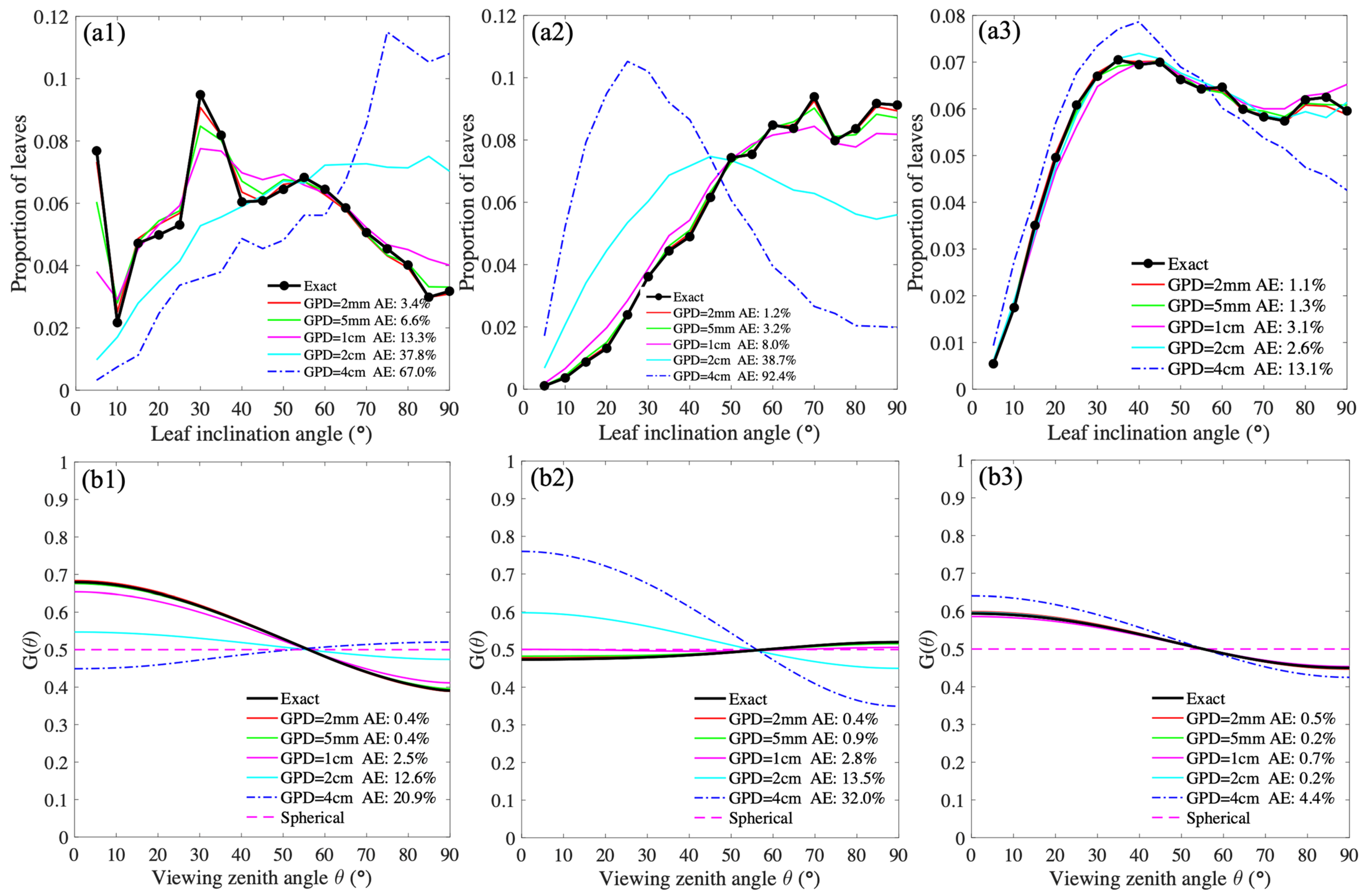
3.1. The Point Density Effect on the LAD and G-Function Calculations Based on CPCs

The LAD and the G-function estimated from CPCs with different GPDs of 2 mm, 5 mm, 1 cm, 2 cm, and 4 cm are illustrated in Figure 4. GPD means the grid point distance; the larger the value is, the lower the point density. The errors in the LAD and G-function show an increasing trend with decreasing point density for all three tree models, and the point density has a greater influence on the LAD. When the GPD is 5 mm (which is easily available in real-world scanning), the errors in the LAD and G-function estimation are 6.9% and 0.4% for Tree1, 3.2% and 0.9% for Tree2, and 1.2% and 0.3% for Tree3, respectively. When the GPD is greater than 1 cm, the error increases greatly, and the result of the 4-cm GPD is illustrated to show the great influence of the point density: the errors in the LAD and G-function estimation are 60.7% and 20.9% for Tree1, 92.4% and 32.0% for Tree2, 13.1% and 4.4% for Tree3, respectively. With the decrease in the point density, the increases in the error for the three trees differ. Nevertheless, the increasing trend generally indicates that the number of points per unit leaf area should be larger than 1 cm−2 (roughly equivalent to GPD = 1 cm) when using the point clouds to estimate the LAD in our studied cases.

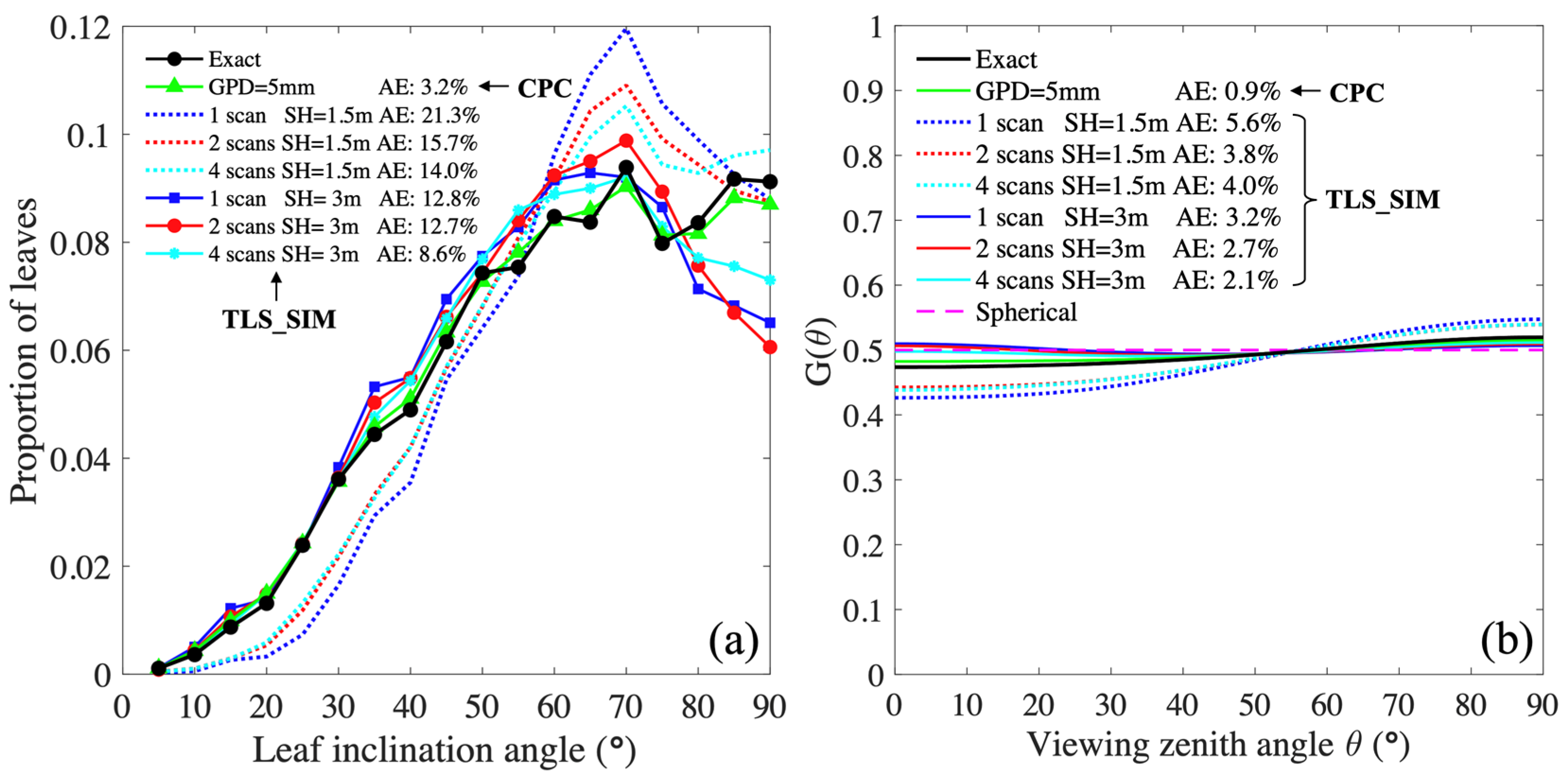
3.2. The Effect of the Number of Scans and Scanner Height on the LAD and G-Function Calculations and the Occlusion Effect

Considering that lower point density leads to larger error, simulated TLS data with an NPD of 5 mm, which is close to the original point spacing (4 mm) were used for further analysis of other influencing factors including the number of scans, scanner height, and the occlusion effect. Figure 5 shows the estimated LAD and G-function for Tree1. Both the calculated CPC with a GPD of 5 mm and the simulated TLS data with an NPD of 5 mm from different scans were used to assess the accuracy of the method. For the calculated CPC, the overall deviation between the estimated value and the true value (AE) is 6.6% for LAD and 0.4% for G-function, respectively. For the simulated TLS, when the scanner height (SH) is 1.5 m, the AEs of the one scan, two, four, and eight scans are 39.4% (19.4%, SH = 3 m), 33.2% (20.9%, SH = 3 m), 41.1% (16.7%, SH = 3 m), and 38.3% (14.5%, SH = 3 m) for the LAD, respectively; and 9.9% (0.6%, SH = 3 m), 7.7% (0.9%, SH = 3 m), 5.9% (0.6%, SH = 3 m), and 10.3% (2.0%, SH = 3 m) for the G-function, respectively. Both the accuracy of the LAD and G-function increased considerably when the SH was doubled. The difference in the LAD between one scan and two scans was 6.2% of the AE; increasing the number of scans additionally does not make the results better in this case because the accuracies of the results from four scans and eight scans are similar. The results show that the scanner height has a greater influence on the accuracy of LAD estimation, when compared with the number of scans.
Taking the results of the LAD and the G-function based on the CPC (with a GPD of 5 mm) as a reference, the occlusion effect causes an AE up to 26% and 14% when the two scans were performed at SHs of 1.5 m and 3 m, respectively. The influence of the occlusion effect is significantly different when the scanner height changes, and the corresponding analysis will be detailed in the Discussion. In addition, eight scans are not considered for the other trees since we found in Tree1 that the differences between the eight scans and the four scans are small.
Figure 6 shows the estimated LAD and G-function for Tree2. Both TH and CD of Tree2 are larger than that of Tree1, but the leaf area density is much lower (see Figure 1). The results of the CPC with a GPD of 5 mm for Tree2 are illustrated, and the method causes an AE of 3.2% for LAD and 0.9% for G-function when applied to the CPC. Regarding the simulated TLS data with an NPD of 5 mm, when the SH is 1.5 m, the AEs of the one scan, two scans, and four scans are 21.3% (12.8%, SH = 3 m), 15.7% (12.7%, SH = 3 m), and 14.0% (8.6%, SH = 3 m) for the LAD, respectively; and 5.6% (3.2%, SH = 3 m), 3.8% (2.7%, SH = 3 m), and 4.0% (2.1%, SH = 3 m) for the G-function, respectively. Both the accuracy of the LAD and the G-function increase when the scanner height is doubled. Taking the result of the LAD and the G-function based on the CPC (with a GPD of 5 mm) as a reference, the occlusion effect causes an AE up to 13% and 10% when two scans were performed with SHs of 1.5 m and 3 m, respectively. Regarding the effect of the number of scans on the LAD, the difference in AE between the one scan and the merged result of the two scans is 5.6% for the LAD and 1.8% for the G-function, when the SH is 1.5 m. The result of the four scans is similar to that of the two scans. The effect of the number of scans has a similar trend when the SH increases to 3 m.
Figure 7 shows the LAD and G-function results for Tree3. The height of Tree3 is 6.5 m, the tallest of all the three tree models. For the CPC with a GPD of 5 mm, the method causes an AE of 1.3% for LAD and 0.2% for G-function. Regarding the simulated TLS data with an NPD of 5 mm, when the scanner height (SH) is 1.5 m, the AE of the one scan, two scans, and four scans is 71.5% (43.8%, SH = 3 m), 64.2% (38.0%, SH = 3 m), and 64.7% (40.9%, SH = 3 m) for the LAD, respectively; and 21.7% (13.3%, SH = 3 m), 19.9% (11.7%, SH = 3 m), and 19.9% (12.6%, SH = 3 m) for the G-function, respectively. Both the accuracy of the LAD and the G-function increase when the SH is doubled. Taking the result of the LAD and the G-function based on the CPC (with a GPD of 5 mm) as a reference, the occlusion effect causes an AE up to 63% and 37% when two scans are performed with SHs of 1.5 m and 3 m, respectively. Both the accuracy of the LAD and the G-function increase considerably when the SH is doubled; however, the results show that relatively accurate results cannot be obtained even if the SH increases considerably when the height of the tree is large. Regarding the effect of the number of scans, both the LAD and G-function calculations show that two scans are better than one scan (an improvement of 7.3% for LAD, and 1.8% for G-function) when the SH is 1.5 m. The difference between the two and the four scans is small (less than 2%). A similar trend was found when the SH was 3 m.

4. Discussion

4.1. The Accuracy Assessment of LAD Estimation

There are two methods used to test the accuracy of LAD estimation in the current studies: manual measurement [18,19] and computer simulation [18,20]. In manual measurement, the number of leaves that can represent the LAD of the tree should be measured. The main difficulties are that manual measurements contain substantial errors that can vary between the individuals performing the measurements [18]. Moreover, the selected leaves should be representative, which is difficult to implement in the field. With the development of computer simulation models [31,32,34], which can realize the simulation of TLS data, the simulated point clouds with a known true LAD were used to assess the accuracy: 23, 33, 43, 53, and 63 disks with a uniform distribution in the volume were used by Bailey and Mahaffee [18], and five trees in the 4th Radiation Transfer Model Intercomparison (RAMI-IV) were used by Vicari et al. [20]. Computer simulation used in this study can avoid the problem of the lack of the true LAD; however, there are some limitations due to the assumptions that are inconsistent with the real-world conditions: (i) simplifying the leaf as two triangles neglects the curvature and complex shape of leaves; (ii) the lack of noise and artifacts in the simulated point clouds is inconsistent with real TLS measurement; (iii) the Lambertian assumption of the leaf optical property; (iv) registration errors using multi-scan data, which were merged directly without suffering errors since they were simulated in the same coordinate system, is not considered; (v) the scanning stations are designed to be regular, with the same scanning distance around a tree; however, establishing the location of the TLS is usually difficult to define in fieldwork, which might be limited by the terrain and environmental conditions. Except for these assumptions which are difficult to avoid in the simulation, there is a problem in evaluating the method using simulated point clouds: it is difficult to distinguish whether the error is caused by incomplete scanning and the uneven points, or the method itself, since the occlusion effect also exists in simulated TLS.
The concept of the CPC was proposed in this paper, which is calculated mathematically and is not influenced by the occlusion effect and the beam divergence of LiDAR. Thus, the CPC was used to evaluate the effect of the occlusion on the LAD, combined with the simulated TLS data. In fact, the influence of the occlusion effect, calculated as the difference between the error of LAD from CPC and simulated TLS data, respectively, also contains the influences of the shooting pattern of the laser scanner and the geometric relationship between the object and the laser pulse. Both the spot size and point spacing increase with increasing distance between the object and the scanner. Moreover, the number of hits varies with leaf orientation to the laser pulse of TLS, [19,27] even though a leaf is not occluded by other objects at all. Nevertheless, the use of CPC provides a way to know the accuracy of the method itself, and it makes it clear that it is the quality of the point clouds data that dominates the reliability of the LAD estimated from TLS in our studied cases. In addition, we believe that the CPC can also be used to validate the accuracy of other methods [17,20], such as the normal vector reconstruction of the adjacent points method and the triangulation method [18].

4.2. Possible Sources of Error in LAD Estimation

In the normal vector calculation, a factor that greatly influences the accuracy is the point density. The higher the point density is, the higher the accuracy of LAD and G-function estimation. Neighboring points are more likely to not be on the same leaf when the point density is low, which yields a large calculation error for the leaf inclination angle. As shown in Figure 4, great changes in both the LAD and the G-function occur as the point density changes. It should be noted that the true LAD curve for Tree2 approximately follows a spherical distribution, but the estimated one is totally different from the true LAD curve when the GPD is 2 cm and 4 cm. This finding indicates that the number of points per unit leaf area should be at least larger than 1 cm−2 (corresponding to GPD = 1 cm, see Table 1 for more details) in our studied cases with leaf length ranging from 8 cm to 13 cm and leaf width from 5 cm to 9 cm. In real measurement, this value should be considered according to the curvature and average size of the leaves. Closely related to the point density, the radius used for spherical search of adjacent points was four times the NPD of the simulated point clouds that was subsampled to an NPD of 5 mm. The setting of the searching radius is a tricky problem. Assuming a fixed NPD, larger radius leads to a higher probability of including points on adjacent leaf, especially for trees with crowded leaves (e.g., the AE (6.6%) computed from the CPC of Tree1 (with the largest leaf area density) is the largest of all the three trees); smaller radius (i.e., less adjacent points) causes the calculation of inclination angle to be more sensitive to the noise (see an experiment (Figure 8) of the influence of the noise on inclination angle calculation, when using different numbers of adjacent points) in real measurement.
An inherent limitation in any optical measurement is that objects occluded from the view of the sensor cannot be measured [18], and several studies have determined that the occlusion effect is a major source of uncertainty in the retrieval of canopy structure variables from TLS measurement [7,37]. Figure 5, Figure 6 and Figure 7 show that the accuracy of the LAD is relatively high for all three CPCs with a GPD of 5 mm: 6.6% for Tree1, 3.2% for Tree2, and 1.3% for Tree3. However, a large difference is found between them when the method is applied to the simulated TLS data with an NPD of 5 mm. For Tree1 which has the largest leaf area density, the error of the LAD still reaches 38.3% even though it had been scanned at eight locations. This indicates that the occlusion effect has a substantial influence on the LAD when the leaf area density is large; in addition, this effect cannot be improved through multiple scanning at the same height. With a height of 3.4 m and a leaf area density of 0.9 m2/m3, Tree2 is between Tree 1 and Tree3, and its calculation accuracy is the highest among them. The LAD error of Tree3 with a height of 6.5 m is the largest (64.2% for two scans), indicating that the influence of the occlusion effect is more serious when the trees are taller. The above results are all obtained with a scanner height of 1.5 m, which is the general height of a TLS tripod and was adopted in other studies [18,20]. It should be noted that the result may be greatly improved (from 64% to 38%) when the scanner height is doubled (3 m). Raising the height of the instrument can reduce the influence of the occlusion effect for tall trees. Larger scanner heights are not considered in this study considering the limitation of the tripod used in current measurements. Furthermore, only factors relevant to the measurement are considered; future study should focus on the wind effect, and the impact of tree structure on LAD estimation.

4.3. Difference between the Effect of Number of Scans and Scanner Location on TLS-Based LAD and G-Function Estimation

The results show that the G-function is less affected by the point density and the occlusion effect compared with the LAD. The AEs in all the cases are all much smaller than those of the LAD. For LAD, the higher the point density is, the better the LAD estimation. We found that the results of the merging of two scans are slightly better than one scan in the results of the three simulated trees, with an improvement of 6.2% for Tree1, 5.6% for Tree2, and 7.3% for Tree3, and the average improvement of the three trees in AE is 6.4%, when the SH is 1.5 m. A similar finding is obtained for a 3-m SH. However, the results are not much improved when the number of scans further increases. This is likely due to the fact that scanning the tree at more locations at the same height does not provide more effective samplings of different inclination angles. Therefore, estimating the LAD of an individual tree by performing two scans is slightly better than just performing a single scan. However, it might be difficult to use joint point clouds obtained in the field from different scanning stations. As can be inferred from the results shown in Figure 8b, the influence of registration error using multi-scan data is non-negligible since inclination angle calculation is very sensitive to generated noise. Future explorations, either focusing on improving the LAD estimation just using high-resolution single-scan point clouds data or estimating LAD (e.g., in case the estimation of azimuth angle is necessary) using data from each scanning station directly and then combining them properly through a weighting method, would be interesting topics. In addition, it is worth noting that if we increase the height of the instrument, we may achieve an improvement in the LAD estimation.
As shown in the previous results, there is great improvement in the LAD of all three tree models when the scanner height changes from 1.5 m to 3 m with one scan: a decrease in the AE from 39.4% to 19.4% for Tree1 (a 20.0% improvement in accuracy), 21.3% to 12.8% for Tree2 (an 8.5% improvement), and 71.5% to 43.8% for Tree3 (a 27.7% improvement). Taking Tree1 as an example, many leaves lie between 0° and 5°; however, the estimated proportion of leaves at angles less than 5° is substantially less than the true proportion when the scanner height is 1.5 m (Figure 5a), indicating that horizontal leaves are scanned less often. However, when the scanner height is doubled (Scan II), the overall LAD estimation accuracies are greatly improved, and the estimated proportion of leaves between 0° and 5° increases considerably compared with the result of Scan I. The possible reasons can be explored from the simplified case in Figure 9. Figure 9 shows four leaves, two of which are horizontal but are at different heights, and the other two pieces are slanted. A simulation was performed to test the effect of the scanning location. Two horizontal circles with a radius of 15 cm are simulated using the DART model. One circle is placed at a height of 1.5 m (leaf①); no point is acquired when scanning from Scan I, and some points are acquired in Scan II (Figure 8b). Similarly, the other circle is placed at a height of 0.5 m (leaf②); more points are acquired with Scan II than with Scan I (Figure 9c) because the angle between the emitted pulses of Scan II and leaf② (β in Figure 9a) is larger than that of Scan I (α in Figure 9a). This indicates that more pulses are incident on leaf② than leaf①. The results of leaf③ and leaf④ are similar to those of leaf① and leaf②, so they are not shown here. We believe that this finding might be a reason for the considerable improvement in the LAD accuracy when the scanner height is increased. The limited sampling capability of TLS at the top of tall trees and the fact that the number of hits is affected by the leaf orientation relative to the view direction of the laser [27] result in some leaves under-represented and some over-represented; increasing the tripod or adding platforms could be a pathway to improvement in such cases.

4.4. Future Research Perspectives

The applicability of TLS in LAD estimation for tall trees is limited because TLS suffers from a lower sampling density towards the top of the canopy [36], considering that the scanner is usually placed on a tripod whose height is limited around 1.5 m [29]. It is possible to fly a rotary-wing unmanned aerial vehicle (UAV) (strictly speaking, it is the remotely piloted vehicle (RPA)) and scan a tree in hemisphere space, which would yield minimal occlusion (Figure 10). As illustrated in Figure 10, Scan I and Scan V can be considered conventional TLS, leaf① is a horizontal leaf located at the same height as the scanner of Scan I and Scan V; as a result, no point on this leaf will be scanned. However, when the UAV laser scanning (UAVLS) system scans from the hemisphere space, the leaf that cannot be viewed by Scan I and Scan V may be scanned at other locations, such as Scan II. Regarding the occlusion between leaves, leaf③ and leaf① cannot be scanned during Scan III because of the occlusion of leaf②, but leaf③ can be scanned during Scan V and leaf① can be scanned during Scan II. When the TLS scans a tree at a fixed position, leaves parallel to the pulse direction can never be scanned. However, the UAVLS system can perform multi-angle scanning at multiple locations, thus ensuring relatively complete scanning of the leaves. A recent development in laser scanning is the deployment of lightweight laser scanners such as RieglVUX-1 on UAV platforms [42,43,44]. UAV laser scanning (UAVLS) is close to TLS in terms of resolution (i.e., point density) [36]. However, currently studies using UAVLS are mostly focused on tree-level, such as the estimation of tree height, crown diameter, canopy volume, above-ground biomass (AGB), and individual tree detection [45,46,47,48]. To the best of our knowledge, there are no leaf-level studies yet. The reason is that the accuracy of UAVLS, which is affected by the range accuracy of the laser scanner and the positional accuracy that is dependent on the Global Navigation Satellite System/Inertial Navigation System (GNSS/INS) unit, is around cm-level. A 5 cm to 6 cm vertical and horizontal accuracy at nadir direction was reported by [49]. If the accuracy can be improved in the future, we believe that UAVLS is promising in LAD estimation due to its great flexibility in scanning. However, the large field of view (FOV) of UAVLS (such as ± 70° used in [49]) leads to a non-uniform sampling as well. Measurement strategy about how to acquire a high-resolution leaf-level point clouds, such as the design of the flying height, flying speed, the FOV, flight line in hemispherical space, etc., is important to ensure the data quality. Although further investigations are beyond the scope of this study, it is a direction which deserves further attention in the future.
This study just focused on the LAD, future explorations on the effect of the influencing factors on the estimation of other parameters that are often estimated from TLS, such as the LAI [50,51], leaf area density [35,52,53], tree volume [54], above-ground biomass (AGB) [55,56], and foliage height diversity (FHD) [57], would be interesting and important topics. Even though these parameters are not a statistic-dependent variable like the LAD, (i) the measurement strategy might have some influence on the gap fraction estimation between the top and bottom part of an individual tree or a canopy, since gap fraction is affected by the laser spot size [29,58], which varies with the range. The uncertainty of gap fraction inevitably affects the LAI and leaf area density estimation; (ii) estimation of tree volume from TLS might be affected by the way of data acquisition, and thus the AGB since it is relevant to the volume [56]; (iii) FHD is a measure of variability in the vertical structure and is affected by the relative amount of vegetation in each strata [57]. Some studies calculate FHD ( F H D = i ( h ( i ) ln ( h ( i ) ) ) based on the number of hits (h(i)) in each vertical layer (i) from single-scan TLS [57]; measuring the tree at different locations might result in different h(i).

5. Conclusions

We study several issues concerned with TLS point clouds-based LAD estimation, including the point density, the scanning numbers, the scanner locations, and the occlusion effect. Simulated TLS data of realistic tree models were used to test the accuracy, and we reached the following conclusions: (i) obtaining simulated TLS data from the computer simulation model is a way to carry out LAD methodological research and validation because the true LAD can be calculated. However, it is difficult to evaluate the accuracy of the method itself because simulated data also suffer from the occlusion effect. The concept of complete point clouds (CPC) was proposed in this paper, from which the theoretical accuracy of the LAD and G-function calculation with different point densities can be evaluated without the occlusion effect. Furthermore, the occlusion effect on the LAD and G-function calculation using TLS point clouds data can be assessed based on the CPC. (ii) The accuracy of LAD estimation is less affected by the method used in this study; however, it is greatly affected by the point density and the occlusion effect. The result becomes better as the point density increases, and the number of points per unit leaf area should be larger than 1 cm−2 (corresponding to a grid point distance of 1 cm) in our studied cases (leaf length × leaf width: 8 cm × 5 cm, 12 cm × 8 cm, 13 cm × 9 cm). Even though the number of points per unit leaf area of 1 cm−2 is just obtained from CPCs, it is helpful in designing scanning distance (s) of TLS to acquire an average point spacing (d, d = 2 · s · tan / 2 ) with a certain scan angle resolution ( ); (iii) increasing the number of scans at different locations at the same height does not result in apparent improvement (there is an average improvement of 6.4% in AE of the three trees using two-scans data than just single-scan data). Future research should focus on improving LAD using high-resolution single-scan data to avoid the influence of registration error when using multi-scan data; (iv) the height of the instrument should be seriously considered for LAD estimation. The occlusion effect is greatly mitigated when the scanner height is two times the traditional height (1.5 m) in our experiments; with a distance of 5 m from the tree locations to the scanner, and the height from the scanner to the bottom of the tree crown of 2.77 m, 2.64 m, and 2.80 m for Tree1, Tree2, and Tree3, respectively. For tall trees with large leaf area density, we should pay special attention to LAD and G-function calculation using TLS point clouds due to the serious occlusion effect.

Author Contributions

Conceptualization, H.J., R.H. and G.Y.; methodology, H.J. and R.H.; formal analysis, R.H. and S.C.; writing—original draft preparation, H.J., R.H., and S.C.; writing—review and editing, G.Y., J.Q., L.L., D.X., X.M.; visualization, F.L.; supervision, G.Y. All authors have read and agreed to the published version of the manuscript.

Funding

This work was supported by the key program of the National Natural Science Foundation of China (NSFC), Grant No. 42090013, 41901288, and the China Scholarship Council, Grant No. 201906040055.

Informed Consent Statement

Not applicable.

Acknowledgments

We gratefully acknowledge the kind help of DART team in the data simulation, and Daniel Girardeau-Montaut in explaining the technical details of CloudCompare. We thank the anonymous reviewers for their helpful and valuable comments that have greatly improved the paper.

Conflicts of Interest

The authors declare no conflict of interest.

References

  1. Yan, G.; Hu, R.; Luo, J.; Weiss, M.; Jiang, H.; Mu, X.; Xie, D.; Zhang, W. Review of indirect optical measurements of leaf area index: Recent advances, challenges, and perspectives. Agric. For. Meteorol. 2019, 265, 390–411. [Google Scholar] [CrossRef]
  2. Pisek, J.; Sonnentag, O.; Richardson, A.D.; Mõttus, M. Is the spherical leaf inclination angle distribution a valid assumption for temperate and boreal broadleaf tree species? Agric. For. Meteorol. 2013, 169, 186–194. [Google Scholar] [CrossRef]
  3. Goel, N.S.; Qin, W. Influences of canopy architecture on relationships between various vegetation indices and LAI and FPAR: A computer simulation. Remote Sens. Rev. 1994, 10, 309–347. [Google Scholar] [CrossRef]
  4. Chen, J.M. Canopy architecture and remote sensing of the fraction of photosynthetically active radiation absorbed by boreal conifer forests. IEEE Trans. Geosci. Remote Sens. 1996, 34, 1353–1368. [Google Scholar] [CrossRef]
  5. Chen, J.M.; Black, T.A. Defining leaf area index for non-flat leaves. Plant. Cell Environ. 1992, 15, 421–429. [Google Scholar] [CrossRef]
  6. Jonckheere, I.; Fleck, S.; Nackaerts, K.; Muys, B.; Coppin, P.; Weiss, M.; Baret, F. Review of methods for in situ leaf area index determination Part I. Theories, sensors and hemispherical photography. Agric. For. Meteorol. 2004, 121, 19–35. [Google Scholar] [CrossRef]
  7. Béland, M.; Widlowski, J.-L.; Fournier, R.A.; Côté, J.-F.; Verstraete, M.M. Estimating leaf area distribution in savanna trees from terrestrial LiDAR measurements. Agric. For. Meteorol. 2011, 151, 1252–1266. [Google Scholar] [CrossRef]
  8. De Wit, C.T. Photosynthesis of leaf canopies. Agric. Res. Rep. 1965, 1–54. [Google Scholar]
  9. Ross, J. The Radiation Regime and Architecture of Plant Stands; Springer: Dordrecht, The Netherlands, 1981; Volume 3. [Google Scholar]
  10. Kimes, D.S.; Kirchner, J.A. Directional radiometric measurements of row-crop temperatures. Int. J. Remote Sens. 1983, 4, 299–311. [Google Scholar] [CrossRef]
  11. Kvet, J.; Marshall, J.K. Assessment of leaf area and other assimilating plant surfaces. Plant Photosynth. Prod. Man. Methods. 1971, 517–555. [Google Scholar]
  12. Wang, W.M.; Li, Z.L.; Su, H.B. Comparison of leaf angle distribution functions: Effects on extinction coefficient and fraction of sunlit foliage. Agric. For. Meteorol. 2007, 143, 106–122. [Google Scholar] [CrossRef]
  13. Goel, N.S.; Strebel, D.E. Simple Beta Distribution Representation of Leaf Orientation in Vegetation Canopies 1. Agron. J. 1984, 76, 800–802. [Google Scholar] [CrossRef]
  14. Campbell, G.S. Derivation of an angle density function for canopies with ellipsoidal leaf angle distributions. Agric. For. Meteorol. 1990, 49, 173–176. [Google Scholar] [CrossRef]
  15. Thomas, S.C.; Winner, W.E. A rotated ellipsoidal angle density function improves estimation of foliage inclination distributions in forest canopies. Agric. For. Meteorol. 2000, 100, 19–24. [Google Scholar] [CrossRef]
  16. Kuusk, A. A fast, invertible canopy reflectance model. Remote Sens. Environ. 1995, 51, 342–350. [Google Scholar] [CrossRef]
  17. Zheng, G.; Moskal, L.M. Leaf Orientation Retrieval from Terrestrial Laser Scanning (TLS) Data. IEEE Trans. Geosci. Remote Sens. 2012, 50, 3970–3979. [Google Scholar] [CrossRef]
  18. Bailey, B.N.; Mahaffee, W.F. Rapid, high-resolution measurement of leaf area and leaf orientation using terrestrial LiDAR scanning data. Meas. Sci. Technol. 2017, 28, 63–76. [Google Scholar] [CrossRef] [Green Version]
  19. Ma, L.; Zheng, G.; Eitel, J.U.H.; Magney, T.S.; Moskal, L.M. Retrieving forest canopy extinction coefficient from terrestrial and airborne lidar. Agric. For. Meteorol. 2017, 236, 1–21. [Google Scholar] [CrossRef]
  20. Vicari, M.B.; Pisek, J.; Disney, M. New estimates of leaf angle distribution from terrestrial LiDAR: Comparison with measured and modelled estimates from nine broadleaf tree species. Agric. For. Meteorol. 2019, 264, 322–333. [Google Scholar] [CrossRef]
  21. Zhao, K.; García, M.; Liu, S.; Guo, Q.; Chen, G.; Zhang, X.; Zhou, Y.; Meng, X. Terrestrial lidar remote sensing of forests: Maximum likelihood estimates of canopy profile, leaf area index, and leaf angle distribution. Agric. For. Meteorol. 2015, 209–210, 100–113. [Google Scholar] [CrossRef]
  22. Hosoi, F.; Omasa, K. Estimating leaf inclination angle distribution of broad-leaved trees in each part of the canopies by a high-resolution portable scanning lidar. J. Agric. Meteorol. 2015, 71, 136–141. [Google Scholar] [CrossRef] [Green Version]
  23. Kuo, K.; Itakura, K.; Hosoi, F. Leaf segmentation based on k-means algorithm to obtain leaf angle distribution using terrestrial LiDAR. Remote Sens. 2019, 11, 2536. [Google Scholar] [CrossRef] [Green Version]
  24. Jin, S.; Tamura, M.; Susaki, J. A new approach to retrieve leaf normal distribution using terrestrial laser scanners. J. For. Res. 2016, 27, 631–638. [Google Scholar] [CrossRef]
  25. Itakura, K.; Hosoi, F. Estimation of leaf inclination angle in three-dimensional plant images obtained from lidar. Remote Sens. 2019, 11, 344. [Google Scholar] [CrossRef] [Green Version]
  26. Liu, J.; Skidmore, A.K.; Wang, T.; Zhu, X.; Premier, J.; Heurich, M.; Beudert, B.; Jones, S. Variation of leaf angle distribution quantified by terrestrial LiDAR in natural European beech forest. ISPRS J. Photogramm. Remote Sens. 2019, 148, 208–220. [Google Scholar] [CrossRef]
  27. Kuusk, A. Leaf orientation measurement in a mixed hemiboreal broadleaf forest stand using terrestrial laser scanner. Trees Struct. Funct. 2020, 34, 371–380. [Google Scholar] [CrossRef]
  28. Shao, J.; Zhang, W.; Mellado, N.; Wang, N.; Jin, S.; Cai, S.; Luo, L.; Lejemble, T.; Yan, G. SLAM-aided forest plot mapping combining terrestrial and mobile laser scanning. ISPRS J. Photogramm. Remote Sens. 2020, 163, 214–230. [Google Scholar] [CrossRef]
  29. Béland, M.; Baldocchi, D.D.; Widlowski, J.L.; Fournier, R.A.; Verstraete, M.M. On seeing the wood from the leaves and the role of voxel size in determining leaf area distribution of forests with terrestrial LiDAR. Agric. For. Meteorol. 2014, 184, 82–97. [Google Scholar] [CrossRef]
  30. Qi, J.; Xie, D.; Yin, T.; Yan, G.; Gastellu-Etchegorry, J.P.; Li, L.; Zhang, W.; Mu, X.; Norford, L.K. LESS: LargE-Scale remote sensing data and image simulation framework over heterogeneous 3D scenes. Remote Sens. Environ. 2019, 221, 695–706. [Google Scholar] [CrossRef]
  31. Lewis, P. Three-dimensional plant modelling for remote sensing simulation studies using the Botanical Plant Modelling System. Agronomie 1999, 19, 185–210. [Google Scholar] [CrossRef]
  32. Bechtold, S.; Höfle, B. HELIOS: A Multi-Purpose Lidar Simulation Framework for Research, Planning and Training of Laser Scanning Operations With Airborne, Ground-Based Mobile and Stationary Platforms. ISPRS Ann. Photogramm. Remote Sens. Spat. Inf. Sci. 2016, III-3, 161–168. [Google Scholar] [CrossRef] [Green Version]
  33. Yin, T.; Gastellu-Etchegorry, J.P.; Grau, E.; Lauret, N.; Rubio, J. Simulating satellite waveform Lidar with DART model. Int. Geosci. Remote Sens. Symp. 2013, 3029–3032. [Google Scholar] [CrossRef]
  34. Gastellu-Etchegorry, J.-P.; Yin, T.; Lauret, N.; Grau, E.; Rubio, J.; Cook, B.D.; Morton, D.C.; Sun, G. Simulation of satellite, airborne and terrestrial LiDAR with DART (I): Waveform simulation with quasi-Monte Carlo ray tracing. Remote Sens. Environ. 2016, 184, 418–435. [Google Scholar] [CrossRef]
  35. Béland, M.; Widlowski, J.-L.; Fournier, R.A. A model for deriving voxel-level tree leaf area density estimates from ground-based LiDAR. Environ. Model. Softw. 2014, 51, 184–189. [Google Scholar] [CrossRef]
  36. Morsdorf, F.; Kükenbrink, D.; Schneider, F.D.; Abegg, M.; Schaepman, M.E. Close-range laser scanning in forests: Towards physically based semantics across scales. Interface Focus 2018, 8, 20170046. [Google Scholar] [CrossRef] [PubMed] [Green Version]
  37. Shao, J.; Zhang, W.; Mellado, N.; Jin, S.; Cai, S.; Luo, L.; Yang, L.; Yan, G.; Zhou, G. Single Scanner BLS System for Forest Plot Mapping. IEEE Trans. Geosci. Remote Sens. 2020, 1675–1685. [Google Scholar] [CrossRef]
  38. Li, L.; Mu, X.; Soma, M.; Wan, P.; Qi, J.; Hu, R.; Zhang, W.; Tong, Y.; Yan, G. An Iterative-Mode Scan Design of Terrestrial Laser Scanning in Forests for Minimizing Occlusion Effects. IEEE Trans. Geosci. Remote Sens. 2020, 1–20. [Google Scholar] [CrossRef]
  39. Wan, P.; Wang, T.; Zhang, W.; Liang, X.; Skidmore, A.K.; Yan, G. Quantification of occlusions influencing the tree stem curve retrieving from single-scan terrestrial laser scanning data. For. Ecosyst. 2019, 6, 1–13. [Google Scholar] [CrossRef] [Green Version]
  40. Myneni, R.B.; Ross, J.; Asrar, G. A review on the theory of photon transport in leaf canopies. Agric. For. Meteorol. 1989, 45, 1–153. [Google Scholar] [CrossRef]
  41. Hu, R.; Bournez, E.; Cheng, S.; Jiang, H.; Nerry, F.; Landes, T.; Saudreau, M.; Kastendeuch, P.; Najjar, G.; Colin, J.; et al. Estimating the leaf area of an individual tree in urban areas using terrestrial laser scanner and path length distribution model. ISPRS J. Photogramm. Remote Sens. 2018, 144, 357–368. [Google Scholar] [CrossRef] [Green Version]
  42. Wallace, L.; Lucieer, A.; Watson, C.; Turner, D. Development of a UAV-LiDAR system with application to forest inventory. Remote Sens. 2012, 4, 1519–1543. [Google Scholar] [CrossRef] [Green Version]
  43. Lin, Y.; Hyyppä, J.; Jaakkola, A. Mini-UAV-Borne LIDAR for Fine-Scale Mapping. IEEE Geosci. Remote Sens. Lett. 2010, 8, 426–430. [Google Scholar] [CrossRef]
  44. Mandlburger, G.; Pfennigbauer, M.; Riegl, U.; Haring, A.; Wieser, M.; Glira, P.; Winiwarter, L. Complementing airborne laser bathymetry with UAV-based lidar for capturing alluvial landscapes. Remote Sens. Agric. Ecosyst. Hydrol. XVII 2015, 9637, 96370A. [Google Scholar]
  45. Yin, D.; Wang, L. Individual mangrove tree measurement using UAV-based LiDAR data: Possibilities and challenges. Remote Sens. Environ. 2019, 223, 34–49. [Google Scholar] [CrossRef]
  46. Wallace, L.; Lucieer, A.; Watson, C.S. Evaluating tree detection and segmentation routines on very high resolution UAV LiDAR ata. IEEE Trans. Geosci. Remote Sens. 2014, 52, 7619–7628. [Google Scholar] [CrossRef]
  47. Liu, K.; Shen, X.; Cao, L.; Wang, G.; Cao, F. Estimating forest structural attributes using UAV-LiDAR data in Ginkgo plantations. ISPRS J. Photogramm. Remote Sens. 2018, 146, 465–482. [Google Scholar] [CrossRef]
  48. Ten Harkel, J.; Bartholomeus, H.; Kooistra, L. Biomass and Crop Height Estimation of Di ff erent. Remote Sens. 2020, 12, 1–18. [Google Scholar]
  49. Lin, Y.C.; Habib, A. Quality control and crop characterization framework for multi-temporal UAV LiDAR data over mechanized agricultural fields. Remote Sens. Environ. 2021, 256, 112299. [Google Scholar] [CrossRef]
  50. Chen, Y.; Zhang, W.; Hu, R.; Qi, J.; Shao, J.; Li, D.; Wan, P.; Qiao, C.; Shen, A.; Yan, G. Estimation of forest leaf area index using terrestrial laser scanning data and path length distribution model in open-canopy forests. Agric. For. Meteorol. 2018, 263, 323–333. [Google Scholar] [CrossRef]
  51. Li, Y.; Guo, Q.; Su, Y.; Tao, S.; Zhao, K.; Xu, G. Retrieving the gap fraction, element clumping index, and leaf area index of individual trees using single-scan data from a terrestrial laser scanner. ISPRS J. Photogramm. Remote Sens. 2017, 130, 308–316. [Google Scholar] [CrossRef]
  52. Soma, M.; Pimont, F.; Allard, D.; Fournier, R.; Dupuy, J.L. Mitigating occlusion effects in Leaf Area Density estimates from Terrestrial LiDAR through a specific kriging method. Remote Sens. Environ. 2020, 245, 111836. [Google Scholar] [CrossRef]
  53. Soma, M.; Pimont, F.; Durrieu, S.; Dupuy, J.L. Enhanced measurements of leaf area density with T-LiDAR: Evaluating and calibrating the effects of vegetation heterogeneity and scanner properties. Remote Sens. 2018, 10, 1580. [Google Scholar] [CrossRef] [Green Version]
  54. McHale, M.R. Volume estimates of trees with complex architecture from terrestrial laser scanning. J. Appl. Remote Sens. 2008, 2, 023521. [Google Scholar] [CrossRef]
  55. Calders, K.; Newnham, G.; Burt, A.; Murphy, S.; Raumonen, P.; Herold, M.; Culvenor, D.; Avitabile, V.; Disney, M.; Armston, J.; et al. Nondestructive estimates of above-ground biomass using terrestrial laser scanning. Methods Ecol. Evol. 2015, 6, 198–208. [Google Scholar] [CrossRef]
  56. Stovall, A.E.L.; Vorster, A.G.; Anderson, R.S.; Evangelista, P.H.; Shugart, H.H. Non-destructive aboveground biomass estimation of coniferous trees using terrestrial LiDAR. Remote Sens. Environ. 2017, 200, 31–42. [Google Scholar] [CrossRef]
  57. Seidel, D.; Ehbrecht, M.; Puettmann, K. Assessing different components of three-dimensional forest structure with single-scan terrestrial laser scanning: A case study. For. Ecol. Manage. 2016, 381, 196–208. [Google Scholar] [CrossRef]
  58. Yin, T.; Qi, J.; Cook, B.D.; Morton, D.C.; Wei, S.; Gastellu-Etchegorry, J.P. Modeling small-footprint airborne lidar-derived estimates of gap probability and leaf area index. Remote Sens. 2020, 12, 4. [Google Scholar] [CrossRef] [Green Version]
Figure 1. Overview of the simulated data. The three-dimensional (3D) tree models generated in OnyxTREE with different structures, and the details of the number of leaves, leaf size, crown diameter (CD), tree height (TH), and leaf area density are shown in (a1a3). Examples of the leaves and leaf structure of the three tree models are illustrated in (b). Each leaf is made up of two triangles with a common edge. (c1c3) are the true leaf angle distribution (LAD) curves, and (d1d3) illustrate the TLS scanning strategy in the Discrete Anisotropic Radiative Transfer (DART) model for the three tree models.
Remotesensing 13 01159 g001
Figure 2. Schematic diagram of the materials and methods. See Section 2.1 for details of the “3D tree models” and “terrestrial laser scanning (TLS) point clouds”, Section 2.2 and Section 2.3 for the leaf angle distribution (LAD) and G-function calculation, Section 2.4 for the “Complete Point Clouds (CPC)”, and Section 2.5 for the “Influencing factors”.
Remotesensing 13 01159 g002
Figure 3. (a) The schematic diagram of the complete point clouds (CPC) calculation and (b) an example of part of a CPC in a tree. Red points are the vertexes of the triangles that make up a leaf, white lines show how the triangles are gridded, and the white points are the calculated grid points and are called a CPC.
Remotesensing 13 01159 g003
Figure 4. The estimated leaf angle distributions (LADs) (a1a3) for Tree1, Tree2, and Tree3, respectively) and G-functions (b1b3) for Tree1, Tree2, and Tree3, respectively) for the three tree models computed from the complete point clouds (CPCs) with different grid point distances (GPDs) (2 mm, 5 mm, 1 cm, 2 cm, and 4 cm): the “Exact” curves in black are the true LADs and G-functions; AE denotes percentage of the overall deviation between the estimated value and the true value, and the corresponding calculations are given in Equations (4) and (5).
Remotesensing 13 01159 g004
Figure 5. The effect of the number of scans and the scanner height on the leaf angle distribution (LAD) (a) and the G-function (b1,b2) for Tree1; (b1,b2) are the results for scanner heights (SHs) of 1.5 m and 3 m, respectively: the “Exact” curves in black are the true LADs and G-functions computed from the three-dimensional (3D) tree model; the green curves are the LAD and the G-function computed from the complete point clouds (CPC) with a grid point distance (GPD) of 5 mm, which can represent the accuracy without the occlusion effect; TLS_SIM denotes simulated TLS point clouds. The scanning strategy is illustrated in Figure 1(d1).
Remotesensing 13 01159 g005
Figure 6. The effect of the number of scans and the scanner height on the leaf angle distribution (LAD) (a) and the G-function (b) for Tree2: the “Exact” curves in black are the true LAD and the G-function computed from the three-dimensional (3D) tree model, respectively; the green curves are the LAD and G-function computed from the complete point clouds (CPC) with a grid point distance (GPD) of 5 mm, which can represent the accuracy of the method without the occlusion effect; TLS_SIM denotes simulated TLS point clouds. The scanning strategy is illustrated in Figure 1(d2).
Remotesensing 13 01159 g006
Figure 7. The effects of the number of scans and the scanner height on the leaf angle distribution (LAD) (a) and the G-function (b) for Tree3: the “Exact” curves in black are the true LAD and G-function computed from the three-dimensional (3D) tree model; the green curve is the LAD and the G-function computed from the complete point clouds (CPC) with a grid point distance (GPD) of 5 mm, which can represent the accuracy of the method without the occlusion effect; TLS_SIM denotes simulated TLS point clouds. The scanning strategy is illustrated in Figure 1(d3).
Remotesensing 13 01159 g007
Figure 8. Influence of the noise on the inclination angle calculation. (a) Schematic diagram of original points (white) with a point spacing of 5 mm on a horizontal plane, and noised points (red) acquired by adding random values on Z coordinates of the original points; (b) influences of different levels of noise (by adding random values with a mean of zero and a standard deviation ( σ ) of 0.5 mm and 1.5 mm) on the inclination angle calculation of point P using a least squares fitting technique. P is originally on a plane with an inclination angle of 0°; the estimated inclination angles of P on the fitted planes with different number of adjacent points increases with the noise level, and the error generally decreases with the increasing number of adjacent points when the noise level is fixed. A total of 100 datasets of the noised points for each noise level (with the same mean and standard deviation) were generated, and each angle shown in (b) is the average angle calculated from the 100 datasets.
Remotesensing 13 01159 g008
Figure 9. The occlusion effect in terrestrial laser scanning (TLS) and the effect of the scanner height (SH) (a) on the scanned points (b,c). Leaf① and leaf② are horizontal, leaf③ and leaf④ are slanted. The leaves are represented by a straight line because they are illustrated from the side. Dashed lines represent pulses emitted by TLS: the black and blue dashed lines are the pulses emitted by Scan I and Scan II, respectively. α and β are the angles between the emitted pulses of Scan I and leaf② and between Scan II and leaf②, respectively, β > α.
Remotesensing 13 01159 g009
Figure 10. Hemispherical scanning of a tree using UAV laser scanning (UAVLS). Leaf① is horizontal, and leaf② and leaf③ are slanted. Dashed lines represent the pulses emitted by the laser scanner: A, B, C and D are parallel to the leaf, indicating that no point can be acquired in these cases, and the rest (in blue) represent pulses that intersect with the leaves, indicating that some points can be acquired through scanning.
Remotesensing 13 01159 g010
Table 1. Sensitivity analysis.
Sensitivity AnalysisComparisonsData
Point densityGrid point distances (GPDs) of 2 mm, 5 mm, 1 cm, 2 cm, and 4 cm; they are equivalent to:
a number of points per unit leaf area of 26.6 cm−2, 4.6 cm−2, 1.4 cm−2, 0.4 cm−2, and 0.2 cm−2
Complete point clouds (CPC)
Number of scansOne scan and the merged point clouds of two, four, and eight scansSimulated TLS data
Scanner height1.5 m, 3 mSimulated TLS data
Publisher’s Note: MDPI stays neutral with regard to jurisdictional claims in published maps and institutional affiliations.

