
A Comparison between Support Vector Machine and Water Cloud Model for Estimating Crop Leaf Area Index

 , , , , , , , , , , , ,
  and
and
Abstract
:
1. Introduction
2. Study Sites and In Situ Data Collection
2.1. Argentina
2.2. Canada
2.3. Germany
2.4. India
2.5. Poland
2.6. Ukraine
2.7. U.S.A.- North Dakota (ND)
3. Satellite Data Acquisitions
4. Methodology
4.1. The Water Cloud Model (WCM)
4.2. The Support Vector Machine (SVM) Model
4.3. Calibration and Inversion of the WCM Model
4.4. Selection of Calibration and Validation Points
5. Results
5.1. Corn
5.2. Soybeans
5.3. Rice
5.4. Wheat
6. Discussion
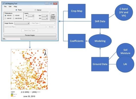
7. LAI Map
8. Conclusions
Author Contributions
Funding
Institutional Review Board Statement
Informed Consent Statement
Data Availability Statement
Acknowledgments
Conflicts of Interest
References
- Shanahan, J.F.; Schepers, J.S.; Francis, D.D.; Varvel, G.E.; Wilhelm, W.W.; Tringe, J.M.; Schlemmer, M.R.; Major, D.J. Use of remote-sensing imagery to estimate corn grain yield. Agron. J. 2001, 93, 583–589. [Google Scholar] [CrossRef] [Green Version]
- Lobell, D.B. The use of satellite data for crop yield gap analysis. Field Crop. Res. 2013, 143, 56–64. [Google Scholar] [CrossRef] [Green Version]
- Kross, A.; McNairn, H.; Lapen, D.; Sunohara, M.; Champagne, C. Assessment of RapidEye vegetation indices for esti-mation of leaf area index and biomass in corn and soybean crops. Int. J. Appl. Earth Obs. Geoinf. 2014, 34, 235–248. [Google Scholar] [CrossRef] [Green Version]
- Dong, T.; Liu, J.; Shang, J.; Qian, B.; Ma, B.; Kovacs, J.M.; Walters, D.; Jiao, X.; Geng, X.; Shi, Y. Assessment of red-edge vegetation indices for crop leaf area index estimation. Remote. Sens. Environ. 2019, 222, 133–143. [Google Scholar] [CrossRef]
- Towers, P.C.; Strever, A.; Poblete-Echeverría, C. Comparison of Vegetation Indices for Leaf Area Index Estimation in Vertical Shoot Positioned Vine Canopies with and without Grenbiule Hail-Protection Netting. Remote. Sens. 2019, 11, 1073. [Google Scholar] [CrossRef] [Green Version]
- Davidson, A.M.; Fisette, T.; McNairn, H.; Daneshfar, B. Detailed Crop Mapping Using Remote Sensing Data (Crop Data Layers), In Handbook on Remote Sensing for Agricultural Statistics (Chapter 4); Delince, J., Ed.; Handbook of the Glob-al Strategy to improve Agricultural and Rural Statistics (GSARS): Rome, Italy, 2017. [Google Scholar]
- Bréda, N. Leaf Area Index. Encycl. Ecol. 2008, 2148–2154. [Google Scholar] [CrossRef]
- Wang, C.; Qi, J.; Moran, S.; Marsett, R. Soil moisture estimation in a semiarid rangeland using ERS-2 and TM imagery. Remote Sens. Environ. 2004, 90, 178–189. [Google Scholar] [CrossRef]
- Álvarez-Mozos, J.; Casalí, J.; González-Audícana, M.; Verhoest, N.E. Correlation between ground measured soil moisture and RADARSAT-1 derived backscattering coefficient over an agricul-tural catchment of Navarre (North of Spain). Biosyst. Eng. 2005, 92, 119–133. [Google Scholar] [CrossRef]
- Bériaux, E.; Lambot, S.; Defourny, P. Estimating surface-soil moisture for retrieving maize leaf-area index from SAR data. Can. J. Remote. Sens. 2011, 37, 136–150. [Google Scholar] [CrossRef] [Green Version]
- Hosseini, M.; McNairn, H.; Merzouki, A.; Pacheco, A. Estimation of Leaf Area Index (LAI) in corn and soybeans using multi-polarization C- and L-band radar data. Remote. Sens. Environ. 2015, 170, 77–89. [Google Scholar] [CrossRef]
- Ahmadian, N.; Borg, E.; Roth, A.; Zölitz, R. Estimating the Leaf Area Index of Agricultural Crops using multi-temporal dual-polarimetric TerraSAR-X Data: A case study in North-Eastern Germany. Photogrammetrie, Fernerkundung. Geoinformation 2016, 5, 301–317. [Google Scholar] [CrossRef] [Green Version]
- Attema, E.P.W.; Ulaby, F.T. Vegetation modeled as a water cloud. Radio Sci. 1978, 13, 357–364. [Google Scholar] [CrossRef]
- Hosseini, M.; McNairn, H.; Mitchell, S.; Davidson, A.; Dingle Robertson, L. Comparison of SAR and Optical Sensors for Biomass Estimations Over Corn Fields. Int. J. Earth Obs. Geoinf. 2019, 83. [Google Scholar] [CrossRef]
- Hosseini, M.; McNairn, H. Using multi-polarization C- and L-band synthetic aperture radar to estimate wheat fields biomass and soil moisture. Int. J. Earth Obs. Geoinf. 2017, 58, 50–64. [Google Scholar] [CrossRef]
- Bériaux, E.; Waldner, F.; Collienne, F.; Bogaert, P.; Defourny, P. Maize Leaf Area Index Retrieval from Synthetic Quad Pol SAR Time Series Using the Water Cloud Model. Remote. Sens. 2015, 7, 16204–16225. [Google Scholar] [CrossRef] [Green Version]
- Mandal, D.; Hosseini, M.; McNairn, H.; Kumar, V.; Bhattacharya, A.; Rao, Y.S.; Mitchell, S.; Dingle Robertson, R.; Davidson, A.; Dabrowska-Zielinska, K. An investigation of inversion methodologies to retrieve the Leaf Area Index of corn from C-Band backscatter. Int. J. Earth Obs. Geoinf. 2019, 82. [Google Scholar] [CrossRef]
- Reisi-Gahrouei, O.; Homayouni, S.; McNairn, H.; Hosseini, M.; Safari, A. Crop Biomass Estimation using Multi-Regression Analysis and Neural Networks from Multitemporal L-band PolSAR data. Int. J. Remote Sens. 2019, 40, 6822–6840. [Google Scholar] [CrossRef]
- Asilo, S.; Nelson, A.; De Bie, K.; Skidmore, A.; Laborte, A.; Maunahan, A.; Quilang, E.J.P. Relating X-band SAR Backscattering to Leaf Area Index of Rice in Different Phenological Phases. Remote. Sens. 2019, 11, 1462. [Google Scholar] [CrossRef] [Green Version]
- McNairn, H.; Jackson, T.J.; Wiseman, G.; Bélair, S.; Berg, A.; Bullock, P.; Colliander, A.; Cosh, M.H.; Seung-Bum, K.; Magagi, R.; et al. The soil moisture active passive validation experiment 2012 (SMAPVEX12): Pre-launch calibration and validation of the SMAP satellite. IEEE Trans. Geosci. Remote Sens. 2015, 53, 2784–2801. [Google Scholar] [CrossRef]
- Jiao, X.; McNairn, H.; Shang, J.; Pattey, E.; Liu, J.; Champagne, C. The sensitivity of RADARSAT-2 polarimetric SAR data to corn and soybean leaf area index. Can. J. Remote. Sens. 2011, 37, 69–81. [Google Scholar] [CrossRef]
- Jonckheere, I.; Fleck, S.; Nackaerts, K.; Muys, B.; Coppin, P.; Weiss, M.; Baret, F. Review of methods for in situ leaf area index determination: Part I. Theories, sensors and hemispherical photography. Agric. For. Meteorol. 2004, 121, 19–35. [Google Scholar] [CrossRef]
- Garrigues, S.; Shabanov, N.; Swanson, K.; Morisette, J.; Baret, F.; Myneni, R. Intercomparison and sensitivity analysis of leaf area index retrievals from LAI-2000, AccuPAR, and digital hemispherical photography over croplands. Agric. For. Meteorol. 2008, 148, 1193–1209. [Google Scholar] [CrossRef] [Green Version]
- Pultz, T.; Crevier, Y.; Brown, R.; Boisvert, J. Monitoring local environmental conditions with SIR-C/X-SAR. Remote. Sens. Environ. 1997, 59, 248–255. [Google Scholar] [CrossRef]
- Bhuiyan, H.A.; McNairn, H.; Powers, J.; Friesen, M.; Pacheco, A.; Jackson, T.J.; Cosh, M.H.; Colliander, A.; Berg, A.; Rowlandson, T.; et al. Assessing SMAP Soil Moisture Scaling and Retrieval in the Carman (Canada) Study Site. Vadose Zone J. 2018, 17, 180132. [Google Scholar] [CrossRef] [Green Version]
- Rowlandson, T.L.; Berg, A.A.; Bullock, P.R.; Ojo, E.R.; McNairn, H.; Wiseman, G.; Cosh, M.H. Calibration Proce-dures for Surface Soil Moisture Measurements during Soil Moisture Active Passive Experiment 2012 (SMAPVEX-12). J. Hydrol. 2013, 498, 335–344. [Google Scholar] [CrossRef]
- Potter, E.; Wood, J.; Nicholl, C. SunScan Canopy Analysis System: Users Manual; Delta-T Devices: Cambridge, UK, 1996. [Google Scholar]
- Kumar, V.; Mandal, D.; Bhattacharya, A.; Rao, Y. Crop characterization using an improved scattering power decomposition technique for compact polarimetric SAR data. Int. J. Appl. Earth Obs. Geoinf. 2020, 88, 102052. [Google Scholar] [CrossRef]
- Dey, S.; Mandal, D.; Robertson, L.D.; Banerjee, B.; Kumar, V.; McNairn, H.; Bhattacharya, A.; Rao, Y. In-season crop classification using elements of the Kennaugh matrix derived from polarimetric RADARSAT-2 SAR data. Int. J. Appl. Earth Obs. Geoinf. 2020, 88, 102059. [Google Scholar] [CrossRef]
- Mandal, D.; Kumar, V.; Ratha, D.; Lopez-Sanchez, J.M.; Bhattacharya, A.; McNairn, H.; Rao, Y.S.; Ramana, K.V. As-sessment of rice growth conditions in a semi-arid region of India using the Generalized Radar Vegetation Index derived from RADARSAT-2 polarimetric SAR data. Remote Sens. Environ. 2020, 237, 111561. [Google Scholar] [CrossRef] [Green Version]
- Mandal, D.; Kumar, V.; Rao, Y.; Bhattacharya, A.; Ramana, K. Experimental Field Campaigns at Vijayawada Test Site; Technical Report MRS2019TR02; Microwave Remote Sensing Lab: Mumbai, India, 2019. [Google Scholar]
- Dabrowska-Zielinska, K. LPVP—Land Products Validation and Characterisation in Support to Proba-V, S-2 and S-3 Mission—ESRIN Contract No. 4000116440/16/I-SBo. 2016. Available online: https://lpvp.eu/ (accessed on 1 February 2021).
- Shelestov, A.; Kolotii, A.; Camacho, F.; Skakun, S.; Kussul, O.; Lavreniuk, M.; Kostetsky, O. Mapping of biophysical parameters based on high resolution EO imagery for JECAM test site in Ukraine. In Proceedings of the 2015 IEEE International Geoscience and Remote Sensing Symposium (IGARSS), Milan, Italy, 26–31 July 2015; pp. 1733–1736. [Google Scholar]
- Waldner, F.; De Abelleyra, D.; Verón, S.R.; Zhang, M.; Wu, B.; Plotnikov, D.; Bartalev, S.; Lavreniuk, M.; Skakun, S.; Kussul, N.; et al. Towards a set of agrosystem-specific cropland mapping methods to address the global cropland diversity. Int. J. Remote. Sens. 2016, 37, 3196–3231. [Google Scholar] [CrossRef] [Green Version]
- Morisette, J.T.; Baret, F.; Privette, J.L.; Myneni, R.B.; Nickeson, J.; Garrigues, S.; Shabanov, N.V.; Weiss, M.; Fernandes, R.A.; Leblanc, S.G.; et al. Validation of global moderate-resolution LAI products: A framework pro-posed within the CEOS land product validation subgroup. IEEE Trans. Geosci. Remote Sens. 2006, 44, 1804–1817. [Google Scholar] [CrossRef] [Green Version]
- Ulaby, F.T.; Batlivala, P.P.; Dobson, M.C. Microwave backscatter dependence on surface roughness soil moisture and soil texture. Part I—Bare soil. IEEE Trans. Geosci. Remote Sens. 1978, 17, 33–40. [Google Scholar] [CrossRef]
- Basheer, I.; Hajmeer, M. Artificial neural networks: Fundamentals, computing, design, and application. J. Microbiol. Methods 2000, 43, 3–31. [Google Scholar] [CrossRef]
- Smola, A.J.; Schölkopf, B. A tutorial on support vector regression. Stat. Comput. 2004, 14, 199–222. [Google Scholar] [CrossRef] [Green Version]
- Camps-Valls, G.; Bruzzone, L.; Rojo-Alvarez, J.L.; Melgani, F. Robust support vector regression for biophysical var-iable estimation from remotely sensed images. IEEE Geosci. Remote Sens. Lett. 2006, 3, 339–343. [Google Scholar] [CrossRef]
- Verrelst, J.; Camps-Valls, G.; Muñoz-Marí, J.; Rivera, J.P.; Veroustraete, F.; Clevers, J.G.; Moreno, J. Optical remote sensing and the retrieval of terrestrial vegetation bio-geophysical properties—A review. ISPRS J. Photogramm. Remote Sens. 2015, 108, 273–290. [Google Scholar] [CrossRef]
- Miller, S.J. The Method of Least Squares, in Brown University. 2006. Available online: https://web.williams.edu/Mathematics/sjmiller/public_html/BrownClasses/54/handouts/MethodLeastSquares.pdf (accessed on 1 February 2021).
- Marquardt, D.W. An Algorithm for Least-Squares Estimation of Nonlinear Parameters. J. Soc. Ind. Appl. Math. 1963, 11, 431–441. [Google Scholar] [CrossRef]
- Wiseman, G.; McNairn, H.; Homayouni, S.; Shang, J. RADARSAT-2 Polarimetric SAR Response to Crop Biomass for Agricultural Production Monitoring. IEEE J. Sel. Top. Appl. Earth Obs. Remote Sens. 2014, 7, 4461–4471. [Google Scholar] [CrossRef]
- Hosseini, M.; Kerner, H.; Sahajpal, R.; Puricelli, E.; Lu, Y.-H.; Lawal, A.; Humber, M.; Mitkish, M.; Meyer, S.; Becker-Reshef, I. Evaluating the Impact of the 2020 Iowa Derecho on Corn and Soybean Fields Using Synthetic Aperture Radar. Remote Sens. 2020, 12, 3878. [Google Scholar] [CrossRef]
- McNairn, H.; Jiao, X.; Pacheco, A.; Sinha, A.; Tan, W.; Li, Y. Estimating canola phenology using synthetic aperture ra-dar. Remote Sens. Environ. 2018, 219, 196–205. [Google Scholar] [CrossRef]
- Bréda, N.J.J. Ground-based measurements of leaf area index: A review of methods, instruments and current controversies. J. Exp. Bot. 2003, 54, 2403–2417. [Google Scholar] [CrossRef]


| JECAM Site | Crop Types | No. of Fields | Total No. of Samples | LAI Sampling Method | Post Processing Techniques | Area |
|---|---|---|---|---|---|---|
| Argentina | Soybeans | 7 | 86 | Hemispherical Photos | CanEye software | 5 km × 8 km |
| Canada | Corn | 14 | 62 | Hemispherical Photos | CanEye software | 30 km × 70 km |
| Soybeans | 32 | 171 | ||||
| Wheat | 21 | 87 | ||||
| Germany | Corn | 3 | 14 | SS1 SunScan Canopy Analysis System | 25 km × 25 km | |
| Wheat | 8 | 32 | ||||
| India | Rice | 17 | 239 | Hemispherical Photos | CanEye software | 18 km × 35 km |
| Poland | Corn | 27 | 54 | LAI 2200C Plant Canopy Analyzers | 17 km × 18 km | |
| Ukraine | Corn | 25 | 42 | Hemispherical Photos | CanEye software | 12 km × 12 km |
| USA-North Dakota | Corn | 2 | 130 | Plant harvesting | LI-3000, Li-Cor Inc | 5 km × 7 km |
| Soybeans | 2 | 181 |
| JECAM Site | Satellite | Year | Acquisition Dates | Incidence Angles |
|---|---|---|---|---|
| Argentina | RADARSAT-2 | 2017 | 23 December | 33.02°–42.45° |
| 2018 | 16 January; 21 January; 17 March | |||
| Sentinel-1 | 2018 | 6 December | ||
| Canada | RADARSAT-2 | 2012 | 12 June; 19 June; 14 July | 21.08°–35.76° |
| 2016 | 15 June; 16 July | |||
| Sentinel-1 | 2016 | 19 July | ||
| Germany | RADARSAT-2 | 2017 | 29 August | 34.23°–47.70° |
| Sentinel-1 | 2015 | 25 March; 18 April; 24 May; 29 June; 11 August; 13 August | ||
| 2016 | 31 March; 6 June; 10 August; 22 August; 12 September; 4 October; 15 October | |||
| 2017 | 20 April; 1 May; 3 June; 15 June; 25 June; 6 July; 27 July; 18 August; 19 August; 29 August | |||
| India | RADARSAT-2 | 2014 | 29 September; 23 October; 16 November; 10 December | 32.39°–44.14° |
| 2018 | 5 July; 22 August; 2 November | |||
| Poland | RADARSAT-2 | 2018 | 4 September; 15 November | 31.63°–45.55° |
| Sentinel-1 | 2016 | 26 April; 5 June; 13 June; 7 July; 26 July; 31 July | ||
| 2018 | 11 April; 8 May; 10 May; 27 June; 28 June; 8 August; 9 August; 4 September; 5 September; 15 November | |||
| Ukraine | RADARSAT-2 | N/A | 32.97°–45.73° | |
| Sentinel-1 | 2016 | 11 April; 9 May; 27 May; 28 June; 8 July; 15 July; 29 July | ||
| USA-ND | RADARSAT-2 | 2018 | 12 June; 6 July; 30 July; 23 August; 16 September; 10 October | 31.61°–46.59° |
| Sentinel-1 | 2017 | 12 June; 17 June; 24 June; 29 June; 6 July; 11 July; 23 July; 30 July | ||
| 2018 | 26 May; 31 May; 7 June; 12 June; 19 June; 24 June; 1 July; 6 July; 13 July; 18 July; 25 July; 30 July; 6 August; 11 August; 18 August; 23 August; 30 August; 4 September; 11 September; 16 September; 23 September; 28 September; 5 October; 10 October; 17 October |
| Crop Type | Total LAI Range () | Total Soil Moisture Range () | LAI Thresholds for the Model Calibrations |
|---|---|---|---|
| Corn | 0.02–6 | 0.05–0.43 | LAI < 2.5, 2.5 ≤ LAI < 5, and 5 ≤ LAI |
| Soybeans | 0.01–5.97 | 0.05–0.48 | LAI < 1.5, 1.5 ≤ LAI < 3, and 3 ≤ LAI |
| Rice | 0.11–4.67 | N/A | LAI < 1.5, 1.5 ≤ LAI < 3, and 3 ≤ LAI |
| Wheat | 1–8.59 | 0.13–0.46 | LAI < 3, 3 ≤ LAI < 6 and 6 ≤ LAI |
| Crop Type | Total Number of Sites | No. of Sites with LAI and Soil Moisture | No. of Calibration Points | No. of Calidation Points |
|---|---|---|---|---|
| Corn | 302 | 130 | 65 | 237 |
| Soybeans | 445 | 171 | 86 | 359 |
| Rice | 239 | 239 | 119 | 120 |
| Wheat | 119 | 119 | 60 | 59 |
Publisher’s Note: MDPI stays neutral with regard to jurisdictional claims in published maps and institutional affiliations. |
© 2021 by Her Majesty the Queen in Right of Canada as represented by the Minister of Agriculture and Agri-Food Canada. Licensee MDPI, Basel, Switzerland. This article is an open access article distributed under the terms and conditions of the Creative Commons Attribution (CC BY) license (https://creativecommons.org/licenses/by/4.0/).
Share and Cite
Hosseini, M.; McNairn, H.; Mitchell, S.; Robertson, L.D.; Davidson, A.; Ahmadian, N.; Bhattacharya, A.; Borg, E.; Conrad, C.; Dabrowska-Zielinska, K.; et al. A Comparison between Support Vector Machine and Water Cloud Model for Estimating Crop Leaf Area Index. Remote Sens. 2021, 13, 1348. https://0-doi-org.brum.beds.ac.uk/10.3390/rs13071348
Hosseini M, McNairn H, Mitchell S, Robertson LD, Davidson A, Ahmadian N, Bhattacharya A, Borg E, Conrad C, Dabrowska-Zielinska K, et al. A Comparison between Support Vector Machine and Water Cloud Model for Estimating Crop Leaf Area Index. Remote Sensing. 2021; 13(7):1348. https://0-doi-org.brum.beds.ac.uk/10.3390/rs13071348
Chicago/Turabian StyleHosseini, Mehdi, Heather McNairn, Scott Mitchell, Laura Dingle Robertson, Andrew Davidson, Nima Ahmadian, Avik Bhattacharya, Erik Borg, Christopher Conrad, Katarzyna Dabrowska-Zielinska, and et al. 2021. "A Comparison between Support Vector Machine and Water Cloud Model for Estimating Crop Leaf Area Index" Remote Sensing 13, no. 7: 1348. https://0-doi-org.brum.beds.ac.uk/10.3390/rs13071348