Article

Inconsistency among Landsat Sensors in Land Surface Mapping: A Comprehensive Investigation Based on Simulation

1
College of Computer and Information Engineering, Xiamen University of Technology, Xiamen 361024, China
2
Big Data Institute of Digital Natural Disaster Monitoring in Fujian, Xiamen University of Technology, Xiamen 361024, China
3
Fujian Key Laboratory of Sensing and Computing for Smart Cities, Xiamen University, Xiamen 361005, China
4
Research Center for Eco-Environmental Sciences, State Key Laboratory of Urban and Regional Ecology, Chinese Academy of Sciences, Beijing 100085, China
5
School of Physics, Huazhong University of Science and Technology, Wuhan 430074, China
6
Jiangxi Key Laboratory of Soil Erosion and Prevention, Jiangxi Institute of Soil and Water Conservation, Nanchang 330029, China
*
Author to whom correspondence should be addressed.
Submission received: 22 February 2021 / Revised: 29 March 2021 / Accepted: 30 March 2021 / Published: 3 April 2021
(This article belongs to the Special Issue Optical Remote Sensing Applications in Urban Areas)

Abstract

:
Comprehensive investigations on the between-sensor comparability among Landsat sensors have been relatively limited compared with the increasing use of multi-temporal Landsat records in time series analyses. More seriously, the sensor-related difference has not always been considered in applications. Accordingly, comparisons were conducted among all Landsat sensors available currently, including Multispectral Scanner (MSS), Thematic Mappers (TM), Enhanced Thematic Mappers (ETM+), and Operational Land Imager (OLI)) in land cover mapping, based on a collection of synthesized, multispectral data. Compared to TM, OLI showed obvious between-sensor differences in channel reflectance, especially over the near infrared (NIR) and shortwave infrared (SWIR) channels, and presented positive bias in vegetation spectral indices. OLI did not always outperform TM and ETM+ in classification, which related to the methods used. Furthermore, the channels over SWIR of TM and its successors contributed largely to enhancement of inter-class separability and to improvement of classification. Currently, the inclusion of MSS data is confronted with significant challenges regarding the consistency of surface mapping. Considering the inconsistency among the Landsat sensors, it is applicable to generate a consistent time series of spectral indices through proper transformation models. Meanwhile, it suggests the generation of specific class(es) based on interest instead of including all classes simultaneously.

1. Introduction

Since the free and open data policy implemented in 2008 [1], increasing applications of the Landsat archive have been publicly reported (especially in earth’s surface dynamics) [2,3]. In particular, time series analyses based on Landsat data have increased significantly due mainly to the free and open data policy as well as other advancements in data processing [3,4]. The archived Landsat data acquired by four sensors are accessible currently, specifically including the Multispectral Scanner (MSS) onboard Landsat 1–5, Thematic Mappers (TM) onboard Landsat 4 and Landsat 5, Enhanced Thematic Mappers (ETM+) onboard Landsat 7, and Operational Land Imager (OLI)/Thermal Infrared Sensor (TIRS) onboard Landsat 8 (Table 1) [5,6]. Ideally, the full advantages of the historical Landsat archives will be achieved in monitoring surface change with proper time series analysis techniques. However, generally, compared against their predecessor(s), successor(s) with more advanced instrument(s) may provide improved land surface information [7] such as the improved performance of Landsat 8 OLI over Landsat 7 ETM+ [8]. Landsat sensors have developed from having four broad channels (of MSS) initially to having eight multi-spectral channels with narrow and well-positioned wavelength ranges (of OLI) [5], which may challenge the time series analyses of the Landsat archives for which data consistency is required. For example, a relatively simple and widely used method in time series analyses (e.g., for land surface change detection), the differencing method, is highly dependent on the consistency of the data (e.g., classification, spectral reflectance or indices at different times) to be compared [3].
To fully take advantage of both the merits of the Landsat program and its free data accessibility and the sustaining developments in its sensors, comparability among different Landsat observations (i.e. MSS, TM, ETM+, and OLI) should be fully understood and improved. However, comprehensive investigations on between-sensor comparability have still been relatively limited when compared against the increasing use of multi-temporal Landsat records for time series analyses, as mentioned in [3]. Meanwhile, sensor-related difference has not been considered, for example, in spectral reflectance or indices [9,10]. In terms of spectral reflectance indices and classification, there have been comparisons separately done between different Landsat sensors. Resulting from the differences in sensors’ characterization, discrepancies were generally observable in spectral reflectance or vegetation indices [7,8,11,12,13,14,15] and in land use classification [9,16,17,18]. Nevertheless, there has been no detailed investigation simultaneously on the consistency issue of all Landsat sensors. This paper aims to investigate comprehensively the characterization and comparison of all Landsat sensors available currently (including MSS, TM, ETM+, and OLI) in land cover mapping, specifically in terms of vegetation spectral indices and classification (Figure 1). Due to the difficulty in collecting contemporaneous observations, a synthesized, multispectral reflectance data collection from hyperspectral records was generated and used in this study. The rest of the paper is organized as follows: Section 2 details the data used and methods implemented. Results on between-sensor comparison among different Landsat sensors in spectral reflectance, spectral indices, and classification, respectively, are shown in Section 3. Discussion and conclusions are presented in Section 4 and Section 5, respectively.

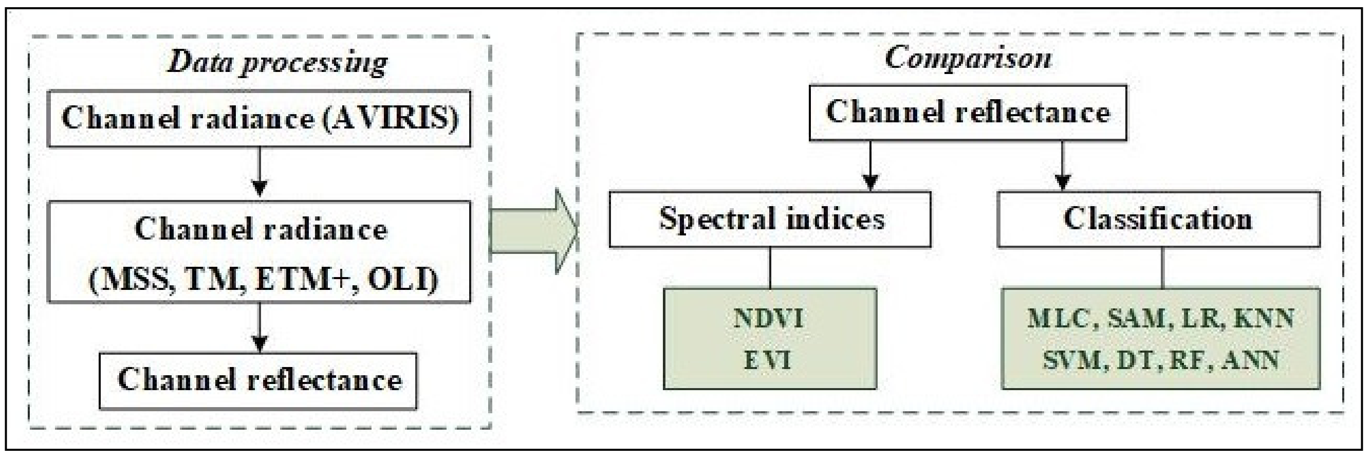
2. Materials and Methods

2.1. Indian Pines AVIRIS Data

The characteristics among different Landsat sensors were investigated and compared comprehensively based on the synthesized multispectral reflectance from an AVIRIS (airborne visible/infrared imaging spectrometer) hyperspectral observation. Due to its well-calibrated property, the AVIRIS was implemented for broadband simulation and comparison [19,20]. The Indian Pines AVIRIS dataset has been widely used as a benchmark for testing classification algorithms in previous investigations [21] due mainly to its well-calibrated radiance and detailed information about ground truth [22]. The ground truth map available for the scene had 16 classes. Considering possible effects associated with sample imbalance, the classes for each of which the number was greater than 500 pixels were selected for classification comparison (Section 2.4). In total, seven classes were selected. Twenty spectral channels (including 104–108, 150–163, and 220) were removed from the initial observation (with 220 spectral channels) due mainly to noise and water absorption. Finally, a total of 200 channels were used in the simulation of multispectral reflectance (see Section 2.2). Information about the calibrated AVIRIS channels is presented in [23].

2.2. Channel Reflectance of Landsat Observations

Two procedures were implemented to generate the synthesized channel reflectance of the Landsat sensors from the Indian Pines AVIRIS data, specifically through (a) obtaining synthesized channel radiance (see Section 2.2.1) and (b) estimating the channel reflectance considering solar irradiance (see Section 2.2.2).

2.2.1. Obtaining Synthesized Channel Radiance

The pixel values of the Indian Pines AVIRIS data are calibrated data (SDV). Accordingly, to retrieve the radiance values (Rad) (in W m 2 sr 1 μ m 1 ), the following operation (Equation (1)) was performed [23]:
R a d i A = ( S D V i A 1000 ) / 10
where S D V i A and R a d i A were the calibrated data and radiance data for the Indian Pines AVIRIS data over channel i.
The integrated channel radiance of the Landsat sensors (i.e., MSS/TM/ETM+/OLI) were assumed as a weighted sum of the AVIRIS channel radiances correspondingly (Equation (2), as in previous investigations [7,14].
R a d Bi L = i ( n W i A R a d i A )
where n W i A (Equation (3)) is the normalized weight for AVIRIS channel i. R a d Bi L is the simulated radiance over channel Bi of the Landsat sensor correspondingly.
n W i A = W i A i W i A
W i A = λ i S λ i E S R F i A ( λ ) S R F Bi L ( λ ) d λ   with   ( λ i C A ( λ Bi S L ,   λ Bi E L ) )
where S R F Bi L ( λ ) is the spectral response function (SRF) (also known as relative spectral response) of channel Bi of the Landsat sensor (i.e., MSS/TM/ETM+/OLI), with the start wavelength and the end wavelength of λ Bi S L and λ Bi E L , respectively. S R F i A ( λ ) is of the AVIRIS channel i, with the start wavelength and the end wavelength of λ i S and λ i E , respectively, and λ i C A is the center wavelength of the AVIRIS channel i. The SRFs of the Landsat sensors were accessed at [6]. Meanwhile, all individual AVIRIS channels’ SRFs were simulated at 1 nm resolution through a Gaussian function using center wavelength and the full width at half maximum, as in previous investigations [7,14]. In the simulation procedure for channel radiance, factors including the sensors’ radiometric properties were not considered in this study.

2.2.2. Estimating the Channel Reflectance Considering Solar Irradiance

The synthesized reflectance over channel Bi was obtained through solar illumination correction Equation (5):
R e f Bi L = π R a d Bi L d 2 / ( E S U N Bi cos ( θ s ) )
where θ s is solar zenith angle and d is earth-sun distance in astronomical units. E S U N Bi is the exo-atmospheric solar irradiance (ESUN) for channel Bi (see Table 1 and Equation (6)). The cosine of the solar zenith angle is equal to the sine of the solar elevation. In this paper, the sun elevation was set as 60° (pi/3 in radians) according to the information retrieved from the USGS EarthExplorer online interfaces under the respective scenes’ metadata, while the earth–sun distance was 1.01557, estimated correspondingly with the acquisition time of the Indian Pines AVIRIS data.
To estimate reflectance, the ESUN is required. Currently, the ChKur solar spectrum profile is used for the Landsat 7 ETM+ channel ESUN values [6]. Meanwhile, the Thuillier solar spectrum profile [24] has been used for the ESUN values of the Landsat sensors previously [25] and also used for Sentinel-2 MSI [26]. The ESUN values have not been provided for the Landsat 8 OLI data product [27]. Instead of using the ESUNs for the Landsat 8 OLI, both the top atmosphere reflectance and surface reflectance could be converted from digital number (DN) records, with scaling factors provided in the metadata [27]. For full comparison among different Landsat sensors, the Thuillier solar spectrum [24] and the ChKur solar spectrum [28] were used to estimate ESUN values for the Landsat 8 OLI channels separately. The integrated solar irradiance over a specific channel (Bi) of the OLI sensor was calculated through the following equation.
E S U N Bi = λ Bi S λ Bi E S R F Bi L ( λ ) E ( λ ) d λ λ Bi S λ Bi E S R F Bi L ( λ ) d λ
where E ( λ ) is the solar irradiance spectrum (i.e., the Thuillier solar spectrum [24] or the ChKur solar spectrum [28]).
The integration procedure (Equation (6)) was achieved through a trapezoid numerical integration [14,29], and the ESUN values for Landsat 8 OLI were estimated based on the selected solar spectrum profile (i.e., ChKur and Thuillier, respectively). For other sensors (i.e., MSS, TM, and ETM+), the ESUN values calculated by using the ChKur solar spectrum [6] and using the Thuillier solar spectrum [25], respectively, are presented in Table 1. Investigations presented are mainly based on channel reflectance using the ChKur ESUNs, and consistency issues relating to different solar spectrum profiles will be discussed (see Section 4.3).

2.3. Comparison of Landsat Observations in Reflectance and Derived Vegetation Spectral Indices

Characterization differences among the Landsat sensors were first demonstrated through the channel reflectance over approximately corresponding spectral regions, as in previous investigations [7,12,14]. Furthermore, two widely used vegetation spectral indices were discussed, including the normalized difference vegetation index (NDVI) [30] and the enhanced vegetation index (EVI) [31,32], which also served as key variables in Landsat higher-level science products [33]. The EVI (Equation (8) was developed initially for sensors with a blue channel [31], while a modified EVI with two channels (named EVI2, Equation (9)) was proposed for sensors without a blue channel [32]. Accordingly, Equation (8) is applicable for TM, ETM+, and OLI [33], and Equation (9) is adopted for MSS.
NDVI = ( R e f n i r L R e f r e d L ) ( R e f n i r L + R e f r e d L )
EVI = 2.5 × ( R e f n i r L R e f r e d L ) ( R e f n i r L + 6.0 R e f r e d L 7.5 R e f b l u e L + 1 )
EVI 2 = 2.5 × ( R e f n i r L R e f r e d L ) ( R e f n i r L + 2.4 R e f r e d L + 1 )
where R e f b l u e L , R e f r e d L , and R e f n i r L are the channel reflectance over the blue, red, and near-infrared regions of a Landsat observation, respectively. For MSS, NIR2 (800–1000 nm) was used as the near-infrared channel in the vegetation indices estimation. Moreover, considering consistency with its successors (i.e., TM), for MSS, the near-infrared channel used for the vegetation index (i.e., NDVI) was discussed in detail [14].
The overall difference of the corresponding variables was measured using the median difference (MdD, Equation (10)) and the median relative difference (MdRD, Equation (11)) [7,14].
M d D i = m e d i a n ( V a r ij S 1 V a r ij S 2 )
M d R D i = m e d i a n ( 2 × ( V a r ij S 1 V a r ij S 2 ) ( V a r ij S 1 + V a r ij S 2 ) × 100 )
where V a r ij S 1 and V a r ij S 2 are corresponding values of sample j (j = 1, 2, …, nn) for the variable V a r i of sensors S1 and S2 (as baseline) respectively, while m e d i a n (   ) is used to get the median value. In comparison, respective variables for the Landsat 5 TM were used as the baselines (references).

2.4. Comparison of Landsat Observations in Land Use Classification

2.4.1. Classifiers Used in Classification Experiments

Several methods used in pixel-based classification were implemented, including the parametric maximum likelihood classifier (MLC), spectral angle mapper (SAM), logistic regression (LR), K-nearest neighbor (KNN), support vector machines (SVM), decision tree (DT), random forest (RF), and artificial neural networks (ANN). Each classifier with the optimal parameter(s) estimated through cross-validation was applied for the corresponding classification experiments. All classification experiments were carried out using Matlab (R2018). A general introduction to the classifiers is as follows:
  • MLC is the most widely used parametric method [34,35]. In fact, MLC is still commonly used in applications and remains a baseline for classification comparison [21,36,37,38,39].
  • SAM is a physically based spectral classification that uses a spectral angle to match pixels to the reference. The smaller angles represent closer matches to the reference [40]. In contrast to conventional MLC, SAM is relatively insensitive to illumination and albedo effects. For the application of SAM, a target pixel was labeled as the same class of a reference which showed the smallest angle (most similarity).
  • LR constructs a separating hyperplane between two data sets through a logistic function to express distance from the hyperplane, which is regarded as a probability of class membership [41]. For application of LR, the class with maximum probability calculated from the sigmoid function was assigned correspondingly.
  • For the KNN method, only the number of neighbors closest to the target pixel is predetermined for classification, whereas for most other classification algorithms, certain parameterizations and the choice of optimal parameter sets are required. In classification through KNN, each unknown sample is directly compared against the training data [42]. Its relative simplicity and robustness make KNN a valuable method when there are limitations in computational resources [39].
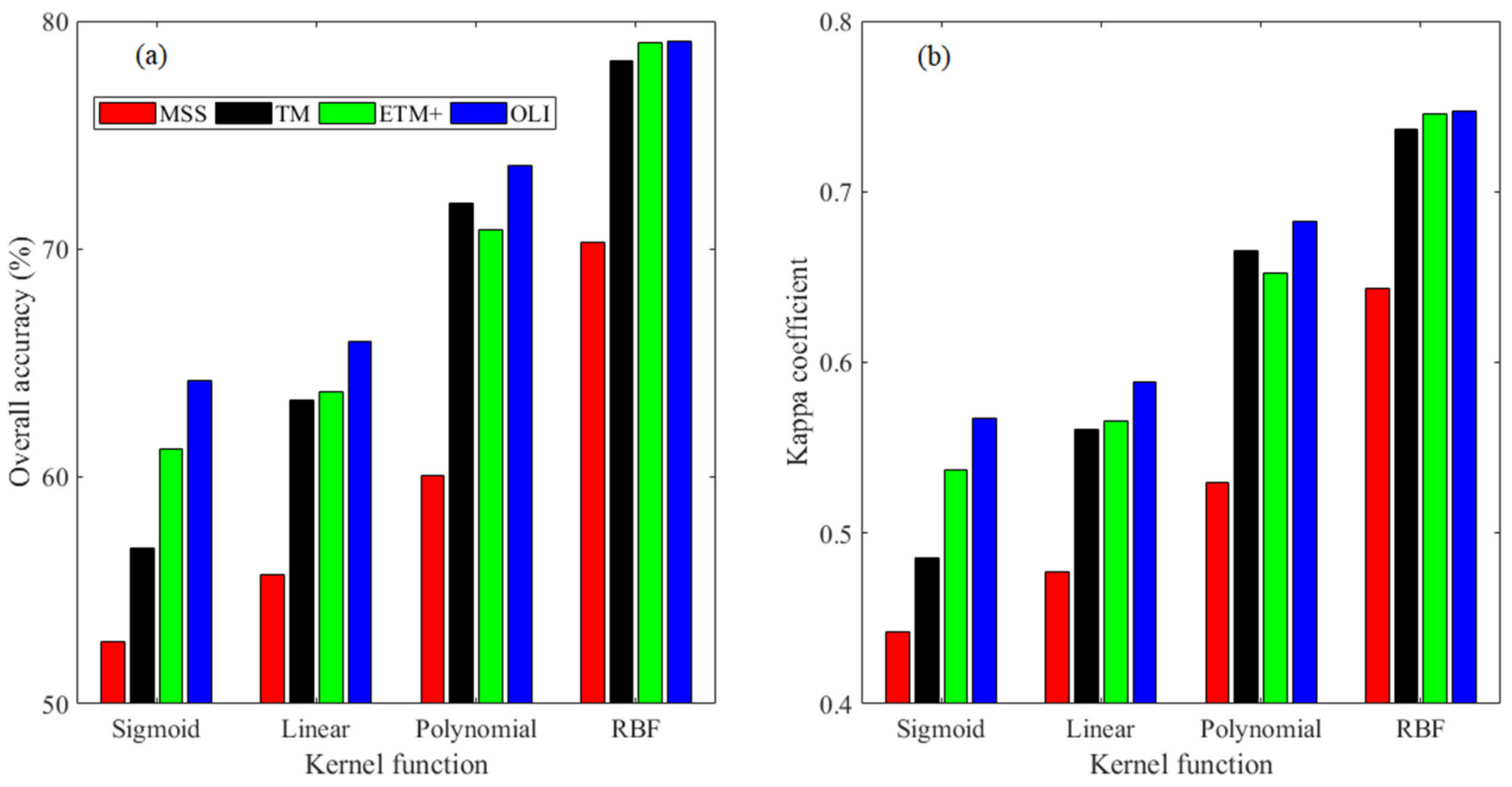
  • The SVM method, based on statistical learning theory, includes a group of non-parametric classifiers [43,44]. SVM is able to produce results with higher accuracy compared with other classifiers [39], even with small training samples [37]. Nevertheless, the performance of SVM is mainly determined by the kernel used and corresponding parameters [36,38,45]. Four kernels widely used, specifically, sigmoid, linear, polynomial, and radial basis function (RBF), also known as Gaussian, were implemented and compared in terms of overall accuracy and Kappa coefficients. According to the experiments on the Indian Pines data, the SVMs with RBF outperformed the SVMs with other kernels (see Section 3.3).
  • A DT classifier is a non-parametric method, which are amongst the most intuitively simple classifiers [21,45]. DT does not use all feature space covariates simultaneously, in that the dataset is recursively divided/partition through a chain of decisions that result from a sequence of tests [21].
  • RF is an ensemble classifier that uses many DTs to overcome the weaknesses of a single DT [46,47,48]. The RF is considered an improved version of bagging, being comparable to boosting in terms of accuracy but computationally much less intensive than boosting [46,47]. The capabilities of RF for land use/cover mapping have been demonstrated [47,48,49].
  • The ANN consists of several highly interconnected processing units (named artificial neurons). The information flow of ANN is stored as connection strengths (called weights) between the neurons [41]. The ability to calculate nonlinear decision boundaries makes the ANN attractive [41]. The accuracy of ANN is dependent on factors such as the number of hidden nodes [50]. In this paper, the ANN with one hidden layer (called a shallow neural network) was implemented for classification, while deep networks [51,52] with increasing trends for application were not considered.
Additionally, the RF can be used to measure the importance of the individual variables for classification [47]. Each tree of the RF is trained using a subset of the variables and a randomly generated subset from the training data. The remaining training samples that are not in the bootstrap sampling for a particular tree, known as the out of bag (OOB) data, can be used in cross-validation to estimate the accuracy (as the generalization error). Accordingly, the importance of a specific variable can be estimated by randomly permuting all the values of the variable in the OOB samples for each classifier followed by a systematical comparison with the classification without permutation [21,46,47]. Based on the importance estimation, individual variables important to classification are identified [21,47,48,53]. The RF was used for classification experiments and variable (i.e., channel reflectance) importance tests.

2.4.2. Training and Accuracy Assessments

It has been recommended as a general rule that a training sample size for each class should not be less than 10 to 30 times the number of variables (e.g., channels) [54]. However, the number of training samples needed should also be determined by considering the complexity of the discrimination problem [55]. Considering the possibly biased effects of imbalanced training samples on the classification model [21], a corresponding equal number of samples for each class were selected through a random strategy. In particular, for the Indian Pines data, 200 samples for each class were selected for training the classifiers, while the rest of the samples (not used for training) were used for accuracy assessment. For this purpose, seven individual classes with larger samples (greater than 500 pixels) were mainly discussed regarding the classification issue, which specifically were Corn-notill (Cn), Corn-mintill (Cm), Grass-trees (Gt), Soybean-notill (Sn), Soybean-mintill (Sm), Soybean-clean (Sc), and Woods (Ws). In total, 1400 samples were selected for training, and 6873 samples were used in testing.
Firstly, to evaluate classification accuracy, widely used indicators based on the error matrix were implemented, including the producer’s accuracy (PA), user’s accuracy (UA), overall accuracy, and Kappa coefficient [56]. Additionally, for individual classes, a harmonic average indicator combining PA and UA was used (HA, Equation (12)), which shows the same meaning as the F1-score [57].
H A = 2 P A × U A P A + U A
Furthermore, pairwise comparison of classification among the Landsat sensors was done using McNemar’s Test [58]. Compared with the traditional z-test commonly used, McNemar’s test is a more precise and sensitive tool in classification comparisons [34,59,60].

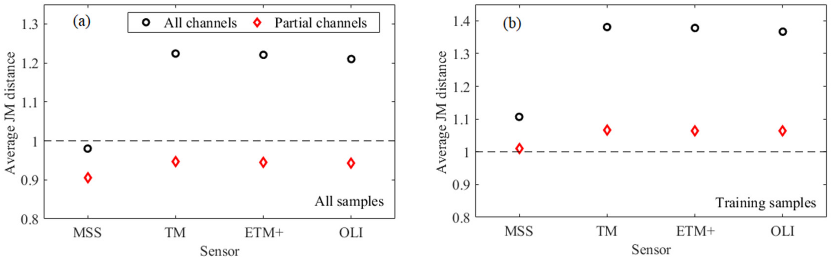
2.4.3. Class Separability Measured by Jeffries–Matusita (JM) Distance

The separability of the major classes over the Indian Pines area was measured using the Jeffries–Matusita (JM) distance [61], which has been considered to be an accurate separability indicator and widely used to define divergence of remote sensing classes [55,62]. The JM distance provides an improved measure of the separation between a pair of probability distributions of classes ( C i and C j ), as given in [61].
JM i j = X p ( x | C i ) p ( x | C j ) 2 d x
For multivariate Gaussian distributions, the JM distance between the classes C i and C j is reduced to the following equation (Equation (14)), with the Bhattacharyya distance (DB) being used [55,61,62]:
JM i j = 2 1 - e DB i j
Meanwhile, the DB between the classes C i and C j is calculated [55,61,62].
DB i j = 1 8 μ C i μ C j T C o v C i + C o v C j 2 1 μ C i μ C j + 1 2 ln ( C o v C i + C o v C j ) / 2 C o v C i C o v C j
where μ C i and μ C j are the mean vector of reflectance values for classes C i and C j respectively, while C o v C i and C o v C j are the corresponding variance–covariance matrices for the two classes. As defined in Equation (14), the JM distance ranges from 0 to 2, with a high value indicating a high level of separability between the pair of classes [62].
Accordingly, the JM distance was calculated for the 21 possible pairs of the seven classes mainly discussed. Furthermore, the average JM distance ( JM a v e ) was used to measure the separability of multiple classes [61].
JM a v e = i = 1 CN j = 1 CN p ( C i ) p ( C j ) J M i j
where CN is the number of classes considered (in this paper, it is seven), and p ( C i ) and p ( C j ) are the a priori probabilities of the classes C i and C j , respectively. To estimate the a priori probability of each class, all valid records for the class were used correspondingly in this paper.
Between-sensor comparison of the JM distance was intended to show the importance of added channels of successors (e.g., TM, ETM+, and OLI) in class separability and classification compared with MSS without channels over the blue and SWIR regions.

3. Results

Based on the synthesized, multispectral reflectance records from the Indian Pines AVIRIS hyperspectral data, the consistency issues among the Landsat sensors were investigated in terms of channel reflectance, spectral indices, and classification. It appeared that the ETM+ and TM observations showed relatively high agreement on channel reflectance and the two derived spectral indices (i.e., NDVI and EVI). Meanwhile, an insignificant difference in classification was likely observed between the ETM+ and TM observations with the same classifier. Using TM as the baseline, the challenges for the time series analysis of the Landsat archive data were mainly associated with MSS (as predecessor) and OLI (as successor) observations. In particular, it showed the inferior performance of MSS in classification resulting from its lack of channels over the SWIR region. Although OLI was superior to TM (e.g., with more channels and superior properties in radiometry), the between-sensor difference in sensor characterization mainly contributed observable biases in channel reflectance and the derived spectral indices.

3.1. Characterization Differences in Channel Reflectance

For the synthesized multispectral reflectance as observed by the Landsat sensors, it appeared that a high degree of agreement between TM and its successors (i.e., ETM+ and OLI) was observable in the blue channel, red channel, and green channel. The between-sensor differences in channel reflectance were significant for OLI, especially over the NIR, SWIR1, and SWIR2 channels. Generally, compared with OLI, ETM+ was more consistent with TM in channel reflectance. Meanwhile, MSS showed consistency with TM over the green and red channels but had a significant bias over the NIR region (Figure 2), consistent with previous findings based on synthesized records from Hyperion hyperspectral profiles [14]. The NIR of MSS presented in Figure 2 is NIR2 (800–1000 nm). Meanwhile, the difference measures for MSS NIR1 (700–800 nm) were MdD (−0.0687) and MdRD (−22.12%), respectively.

3.2. Consistency among the Landsat Sensors in Vegetation Spectral Indices

As previously shown, between-sensor differences in the reflectance of individual channels are especially important when considering derived spectral indices, which usually depend on the reflectivity contrast between channels (e.g., NDVI) [7,14,29]. However, a complex relationship exists between the individual channel biases and corresponding spectral indices such that amplified between-sensor differences in spectral indices are more likely observed [13,29].
General agreement is presented between ETM+ and TM on the two vegetation indices, while ETM+ shows a slightly greater average (Figure 3). OLI obviously shows positive discrepancies with MdD values about 0.04 and 0.07 for NDVI and EVI, respectively. For the vegetation spectral indices of MSS presented in Figure 3, the NIR2 (800–1000 nm) was used in the estimation. Meanwhile, the difference measures for MSS NIR1-based NDVI were −0.0980 (MdD) and −23.19% (MdRD) respectively, and for NIR1-based EVI were −0.3096 (MdD) and −56.64% (MdRD) respectively. Findings based on spectral libraries also demonstrated the relatively significant differences between OLI and its predecessors (i.e., TM and ETM+) in spectral indices [13,29]. Furthermore, as Figure 3 shows, the between-sensor difference in EVI is generally more significant than the difference in NDVI. The most significant differences in EVI were for MSS, mainly caused by the revised version (EVI2) used for EVI estimation without blue channel reflectance. It suggested that direct application of the revised EVI model (EVI2) to MSS was likely questionable, especially when time series analysis was intended based on all valid Landsat archived data. Accordingly, considering the ineffectiveness of EVI2 for MSS, an applicable transformation model was required before time series analysis [7,14].

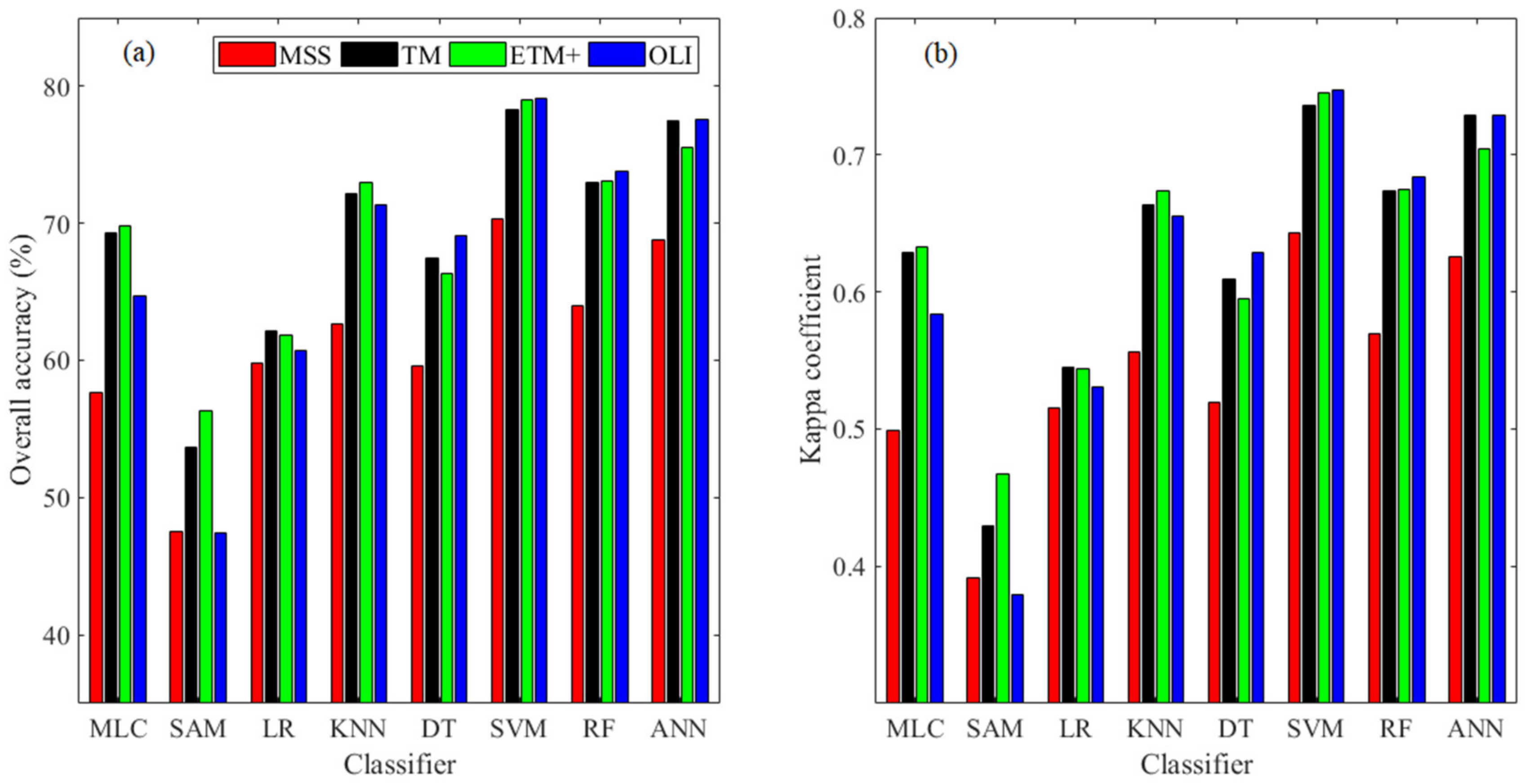
3.3. Comparison of General Classification Results

Land cover mapping is one of the most important applications of remotely sensed imagery acquired by satellite, especially for Landsat images [63]. According to previous investigations [21,39], eight classifiers (see Section 2.4.1) widely applied for pixel-based classification were used. Classification results of each sensor observation were obtained through individual classifiers with optimum parameter(s) using the channel reflectance as inputs without any other procedures or ancillary data. The results for SVM with RBF (radial basis function) kernel were presented. Comparability among classification results obtained from the Landsat sensors was investigated. However, it is worth noting that this investigation did not aim to find out the classifier(s) most suitable for land cover/use mapping.
Overall accuracy and Kappa coefficients as general measures of classification accuracy [56] are shown in Figure 4. It appeared that classification accuracy was generally dependent on methods and sensors (or observations). As mentioned above, for SAM, the final type assigned to a pixel was that of a referencing spectrum with the minimum spectral angle. In SAM, the average spectrum of training samples (for each class) served as the referencing spectrum (also called endmember). The performance of SAM for hard classification was likely affected by the referencing spectrum and spectral mixture. Accordingly, in this case, the SAM showed the worst performance (Figure 4). On average, SVM with RBF kernel outperformed other classifiers, with overall accuracy being approximately 80% when TM and its successors (i.e. ETM+ and OLI) were considered. ANN and RF showed slight inferiority to SVM with RBF kernel. The findings showed consistency with major comparison cases as summarized in [39] in that SVM always achieved the greatest accuracy in terms of classification. RF as an ensemble method outperformed DT with an increase of about 10% in overall accuracy. Meanwhile, two traditional classifiers (i.e., MLC and KNN) generated moderately accurate results, with overall accuracy being about 70% when TM and its successors (i.e. ETM+ and OLI) were considered. Particularly, KNN outperformed other classifiers except three non-parametric classifiers (i.e., SVM with RBF kernel, ANN, and RF) despite its simplicity, showing consistency with previous findings [39].
The McNemar’s test results are shown in Table 2, using TM-based classification as the baseline, correspondingly. Obviously, classification accuracy for MSS observation was lower than TM-based classification regardless of the classifiers investigated. The classification difference between TM and its successors (i.e., ETM+ and OLI) varied with classifier. For example, more accurate results were generated from ETM+ observations when SAM, KNN, SVM, and ANN were separately implemented. Meanwhile, insignificant difference was observed between the classification results from the ETM+ observation and the TM observation, respectively, when other classifiers (i.e., MLC, LR, DT, and RF) were used (Table 2). Nevertheless, the performance of SVM was dependent on kernel function [36,38,45]. Significant accuracy differences among SVMs with different kernels were presented, varying about 20% in overall accuracy and 0.25 in the Kappa coefficient, respectively (Figure 5). Compared against SVM with RBF, SVM with sigmoid showed the poorest performance, which was even less effective than LR and MLC (see Figure 4 and Figure 5). It was consistent with previous investigations in [38] that SVM with RBF showed the best performance in our experiments. However, as shown in [50], two SVMs with other kernels (i.e. polynomial and linear) outperformed SVM with RBF in land use mapping. Therefore, the selection of kernel function followed by the model parameters was a crucial step in classification [38,50].
Furthermore, the optimal parameter(s) of a specific classifier varied more or less among different Landsat observations. For example, for SVM with RBF, the optimal values for “cost” and “gamma” (two parameters) varied at (60, 3000) and (60, 250), respectively, among the Landsat observations. When the optimal parameters of SVM with RBF for TM were implemented for other sensors, the overall accuracy was reduced to about 2.60%, 0.48%, and 0.44% for MSS, ETM+, and OLI, respectively, while the decreases in the Kappa coefficient were about 0.03, 0.01, and 0.005, correspondingly. It suggested that the trained model was not exactly transferable between different Landsat sensors’ observations, especially between MSS and its successors. Consequently, more training tests are necessary for each observation.
In summary, the findings suggest that classification is potentially affected by the sensor observations and classifiers used, which challenges classification consistency among different Landsat observations (sensors) and affects the time series analyses (e.g., change detection) followed by. Furthermore, the performance variation of a classifier among different observations, along with the corresponding varied optimum parameter(s), may further burden general users in the application of machine learning methods (e.g., in remote sensing classification).

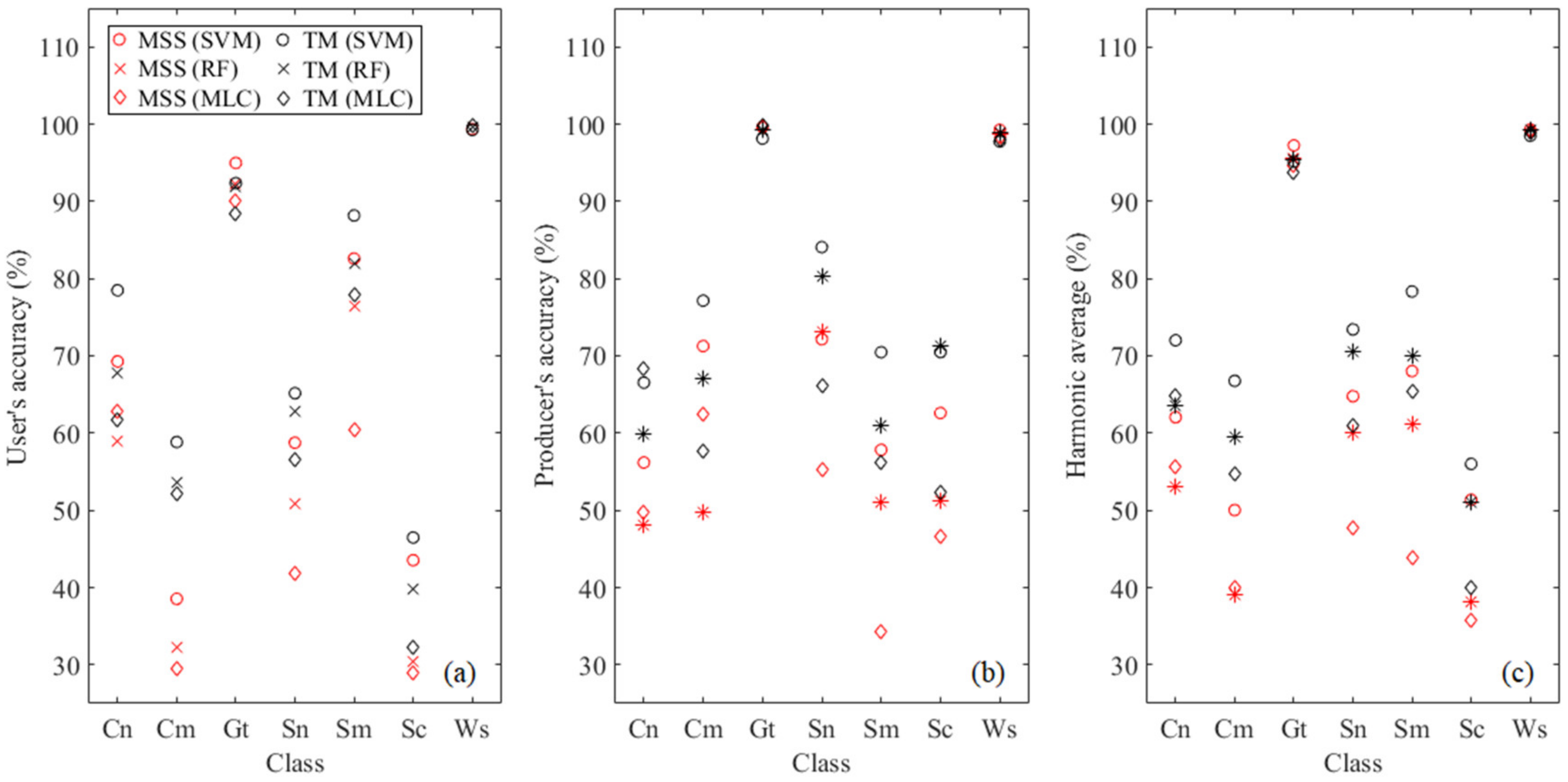
3.4. Comparison of Individual Classes

The classification results for TM and MSS respectively obtained with specific classifiers (i.e., MLC, RF, and SVM) were compared in detail for individual classes. It appears that for the Indian Pines area, observation showed relative importance in classification for most classes (Figure 6). Improvements by using TM were significant for classes Corn-mintill, Soybean-notill, and Soybean-mintill. In particular, for SVM with RBF, class Corn-mintill was obtained at a relatively low accuracy level with MSS. By using TM, the user’s accuracy increased to 60%, while the producer’s accuracy increased about 6% (approximately from 71% to 77%). Generally, the improvements for a specific class were dependent upon the method considered (Figure 6). For MLC, significant improvements for class Soybean-notill were observed in the user’s accuracy (approximately from 60% to 78%) and producer’s accuracy (approximately from 34% to 56%). On the contrary, for SVM with RBF, relatively smaller accuracy improvements were contributed by TM observation. Meanwhile, both methods and observations had negligible effects on the accuracy of two classes (i.e., Grass-trees and Woods), which was possibly associated with the fact that the spectral separability of the classes was large even though MSS observation was used (see Table 3).

4. Discussion

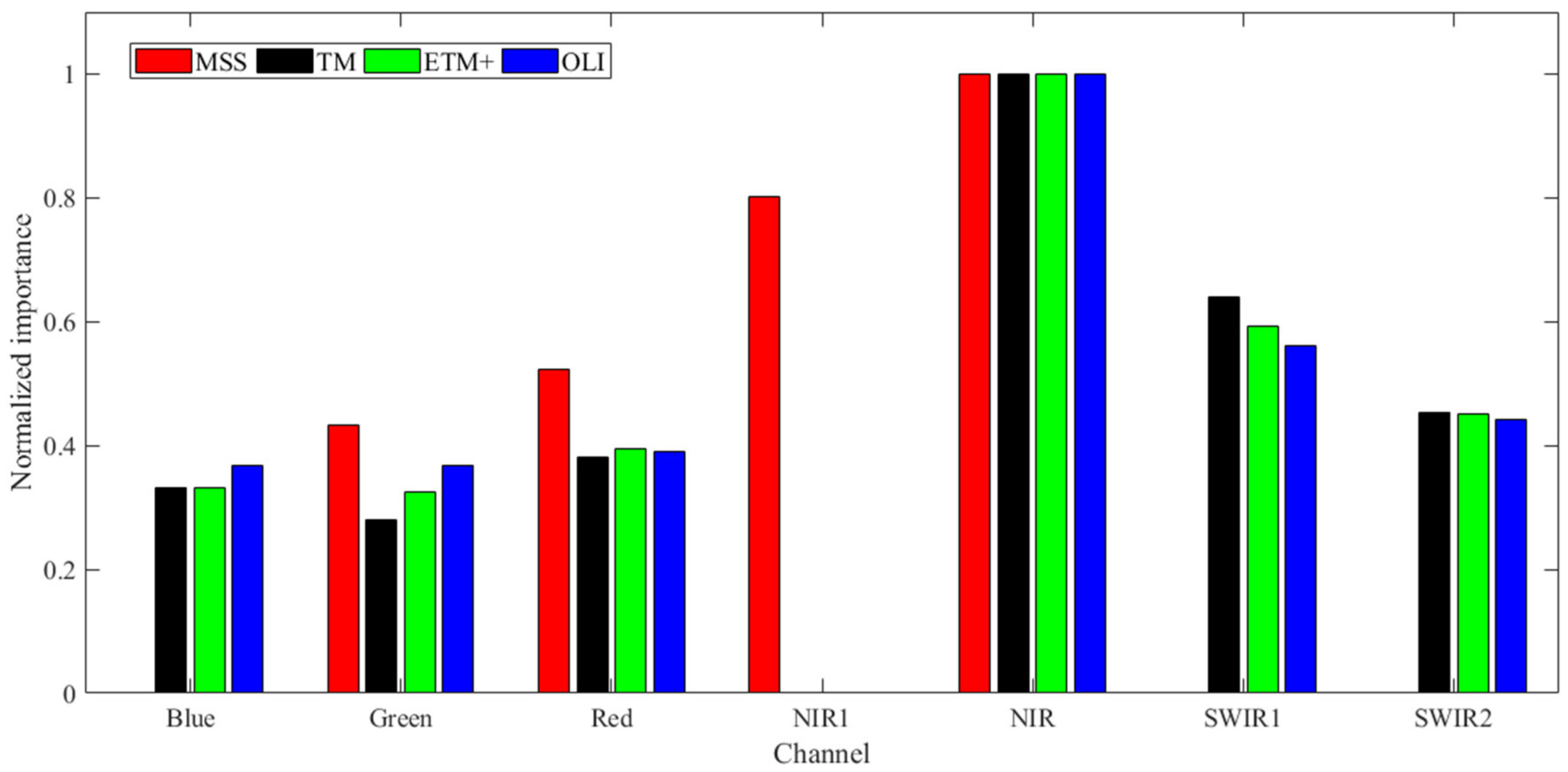
4.1. Contribution of Sensor Characterizations to Classification

Classification was generally improved through more advanced observations (i.e., TM vs. MSS) and classifiers (i.e., SVM with RBF vs. MLC), while the improvement also related to specific categories (Figure 6). The differences in accuracy among individual classes were mainly associated with spectral separability (Table 3).
On average, the JM distance of TM and its successors (i.e., ETM+ and OLI) was larger (with a difference of about 0.30) than the JM distance of MSS (Figure 7). The differences in JM distance were mainly contributed by the two SWIR channels (i.e., SWIR1 and SWIR2) of TM and its successors (i.e., ETM+ and OLI). Meanwhile, the difference in JM distance related to the spectra samples used (see “Training” and “All”). The class separability was calculated under two conditions separately, including “All channels” and “Partial channels” (Figure 7). Specifically, under “Partial channels”, channels except the NIR1 (700–800 nm) were considered for MSS, while for TM, ETM+, and OLI the four channels within visible and NIR regions (including blue, green, red, and NIR) were considered for measuring the JM distance. The increased JM distance explained the improved classification, regardless of classifiers used (Figure 4 and Figure 6). The inter-class JM distances of all pairs increased significantly by using TM instead of MSS, except the pairs of classes Grass-trees and Woods (Table 3). The classes Grass-trees and Woods were highly separable from other classes, with the JM distance approximating to the maximum (2.0) regardless of sensor observations. Accordingly, the classification accuracy for classes Grass-trees and Woods was significantly high, even though MSS observation was used with MLC (Figure 6). Furthermore, the increase in JM distance varied with pairs, which largely contributed to the accuracy variation of individual classes. In particular, with TM observation, class Corn-mintill had a low JM distance (less than 1.0) from the two classes Soybean-mintill and Soybean-clean, whereas it had a relatively high JM distance (approximately 1.5) from the classes Corn-notill and Soybean-notill. Accordingly, with TM observation, for class Corn-mintill, the inter-class misclassification from the classes Corn-notill and Soybean-notill decreased, whereas the confusion with the classes Soybean-mintill and Soybean-clean even increased. It is noteworthy that, in addition to MLC as the conventional parametric classifier, the JM distance was also an effective indicator of class separability for other non-parametric classifiers (e.g., SVM and RF) that are not based on probability theory.
The relative importance of the two SWIR channels (of TM, ETM+, and OLI) was also demonstrated through an RF test (Figure 8). While the NIR channel(s) was (were) showing the most importance in classification over the Indian Pines area, the two SWIR channels were relatively more significant than the channels in the visible region (i.e., including the blue, green, and red channels). In fact, the relative importance (most significant variables) of the MSS NIR2 channel (800–1000 nm) was shown in mapping over a mountainous area in Colorado [47], while the TM NIR and SWIR1 channels were more significant for Level 1 Wetlands mapping in northern Minnesota [53]. The two added SWIR channels of TM and its successors (i.e., ETM+ and OLI) contribute a lot to enhancing inter-class separability and to improving classification, consequently.

4.2. Sensor Characterization and Classifier on Classification

In this investigation, classification experiments were done using channel reflectance as the inputs (in a straightforward manner) without considering additional processes for feature extraction and selection. Findings based on JM distance and RF test demonstrated the channels with relative importance in classification, including those over the NIR, SWIR, and red (Table 3 and Figure 8), which was consistent with other investigations [47,53]. Because of a lack of channel(s) within the SWIR region, MSS was less capable of land surface mapping compared with its successors (i.e., TM, ETM+, and OLI) (Figure 4). However, as mentioned in Figure 4, for TM observation, when even the mostly accurate classification (through SVM with RBF) is considered, both overall accuracy and particular accuracy of individual classes do not meet the classification requirements advocated in [64]. Meanwhile, compared against the results based on original AVIRIS hyperspectral data with the same classifiers (e.g., SVM with RBF and RF) in [21], the results obtained from the Landsat observations were relatively less accurate, showing the advantage of hyperspectral (i.e., AVIRIS) data over multispectral data (i.e. MSS, TM, ETM+, and OLI) in characterizing and discriminating land surface properties. Additionally, compared with MSS, the successors (i.e., TM, ETM+, and TIRS of Landsat 8) had added thermal infrared channel(s). The importance of thermal channels was shown previously in land surface mapping [53,65]. Due mainly to an incapability to synthesize thermal observations from the AVIRIS data, the effects of thermal channel(s) were not investigated in this paper. Obviously, the sensor characterizations (i.e., in spectral regions, spectral response function, and the number of channels) are important for classification.
As shown by overall accuracy, on average, classifiers and observations show comparable importance in classification. For example, for MSS, the difference in overall accuracy was about 13%, between the classification results obtained through SVM with RBF and MLC (Figure 4). Meanwhile, the between-sensor differences (TM minus MSS) in overall accuracy were about 12% and 8% for MLC and SVM with RBF, respectively. However, for individual classes, the relative importance of classifiers and observations changed (Figure 6). In particular, for class Corn-mintill, with MSS observation, the accuracy differences between SVM with RBF and MLC were about 8% and 9%, respectively, in user’s accuracy and producer’s accuracy. At the same time, the between-sensor (TM minus MSS) differences in user’s accuracy were 20% and 23% for SVM with RBF and MLC, respectively, and in producer’s accuracy, were 6% and −5%, correspondingly. The fact that the accuracy of individual classes generally varied with sensor observations and classifiers (Figure 6) was confirmed by previous findings that conclusions for the comparison of classifiers among different case studies were always inconsistent [21,39]. With a specific classifier (e.g., SVM), the performance depended upon model parameters. For SVM methods, the selection of optimum kernel function and its parameters were the major issues that largely affected their performances [38]. However, the optimum parameters usually changed with observations and were not transferable readily (see Section 3.3).

4.3. Solar Spectrum Selection

Results mentioned above were mainly based on the ESUN values calculated using the ChKur solar spectrum [28] (see Table 1). The difference in the ESUN values varied with sensors and channels, correspondingly. Generally, the ChKur based ESUN values were relatively larger over the green and red channels, while the values were relatively smaller over the blue, SWIR1, and SWIR2 channels. The minor difference in ESUN was for the NIR channel(s).
Additionally, the effects of the ESUN differences on channel reflectance and the derived spectral indices were investigated. As derived from Equation (5), the relative difference (RD) in reflectance over a specific channel (Bi) is directly determined by the relative difference of the ESUN bias correspondingly.
RD _ R e f Bi = - Δ E S U N Bi E S U N Bi × 100 %
where Δ E S U N Bi is the residual value between the ESUN values based on ChKur and Thuillier (ChKur minus Thuillier), while E S U N Bi is the ChKur based ESUN. The equation uses the Thuillier based reflectance as the baseline.
The ChKur based reflectance was generally greater than the Thuillier based reflectance over the blue, SWIR1, and SWIR2 channels, with the most significant bias (positive) being over the SWIR2 channel (Figure 9). Relatively smaller reflectance over the green and red channels was obtained using the ChKur based ESUNs. In terms of channel reflectance estimation, OLI was relatively more sensitive to ESUN values over most channels, except the NIR and SWIR1. Meanwhile, greater NDVI was obtained when ChKur based ESUN values were used, regardless of the sensor considered (Figure 9). Significant biases in NDVI caused by different ESUN values were observed for MSS, with a MdD of 0.0100 and MdRD of 2.67%.
For channel reflectance, the ESUN related bias was more significant than the between-sensor difference, especially over the Blue and Red channels, which showed dependency on the sensor (Figure 2 and Figure 9). In particular, for ETM+, the ESUN related bias was more significant over all channels. Accordingly, as previously recommended, for comparisons among sensors, users need to verify that the same solar spectrum is used for all sensors [25,66].

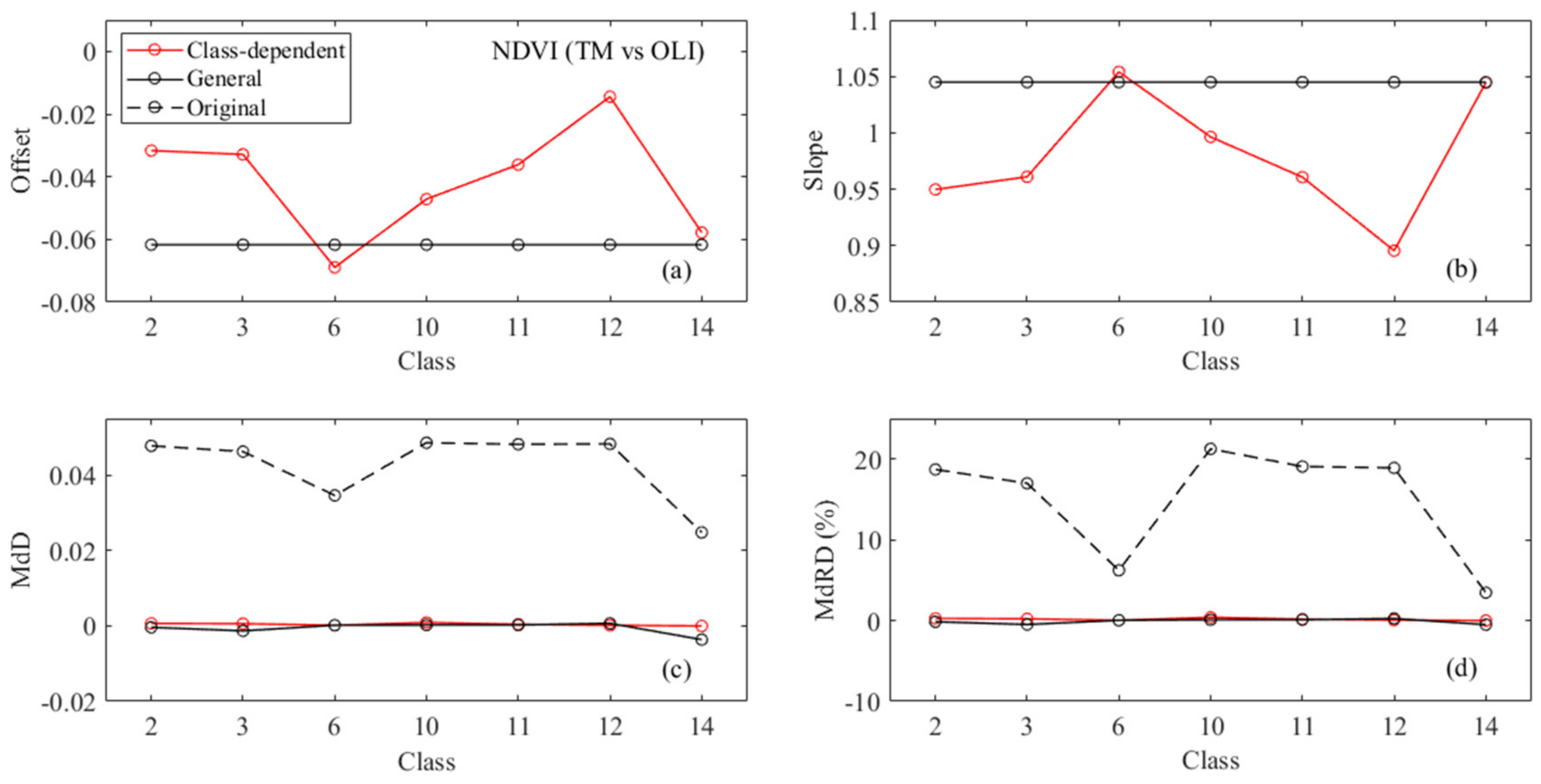
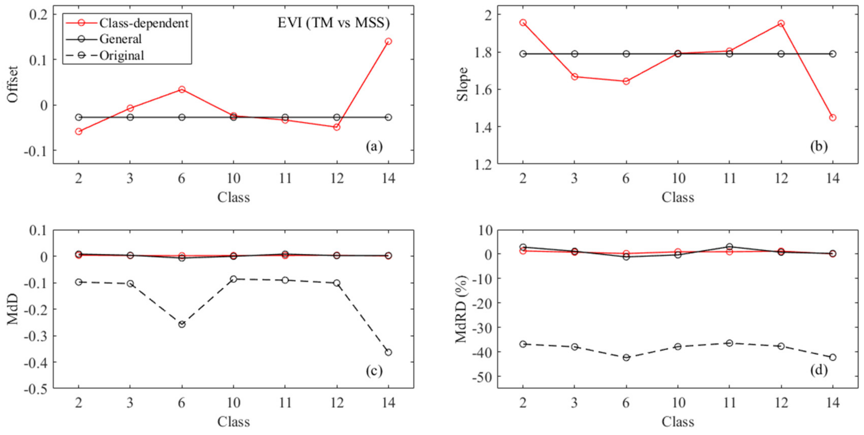
4.4. Improving Consistency among the Landsat Sensors in Channel Reflectance and Vegetation Spectral Indices

Due mainly to the differences in sensor characterization, biases in channel reflectance and two vegetation indices were observed among the Landsat sensors (Figure 2 and Figure 3), challenging time series analyses for which consistent records were required. For channel reflectance and derived spectral indices, a linear transformation model was considered to improve comparability between different sensors [7,12,14]. The comparability improvements in NDVI and EVI through transformation were discussed. In particular, two cases were demonstrated: the NDVI transformation for TM and OLI (Figure 10) and the EVI transformation for TM and MSS (Figure 11). In addition to a general model (“General”, a uniform model for all classes) as discussed previously [7,12,14], individual models for each class (called “Class-dependent”) were obtained. The consistency of spectral indices between two sensors (e.g., NDVI of TM and OLI) was improved significantly through the transformation, either by using a general model or a class-dependent model (Figure 10 and Figure 11). On average, the general model was comparable with the class-dependent method while showing relative insufficiency for specific classes. For example, the relative insufficiency of the general model is observable for classes Corn-mintill and Woods on NDVI consistency (Figure 10), while it is observable for classes Grass-trees and Soybean-mintill on EVI consistency (Figure 11). It suggests that consistency between different sensors in spectral indices is able to be improved through the class-dependent method. However, detailed and accurate land surface classification is usually inaccessible. Accordingly, the general model, which is effective for most areas/samples, is considered applicable in practice [7,12,14].

4.5. Improving Classification Consistency among the Landsat Sensors

Our experiments suggest that classification based on a single observation through ordinary procedures (i.e., using multispectral reflectance directly as the input) is impossible for meeting the requirements for application. Improvements for a single (or a mono-temporal) observation are possibly obtained through different means, such as the inclusion of additional data from other sources [47,53,67,68], multi-temporal observations by the same sensor [69,70,71], extracted indices and features [69,72,73], post processes by manual interpolation [34] or logically knowledge-based rules [70,74,75], and advanced classifiers and strategies [63]. For example, multiple features were used in mapping global land cover, including channel reflectance, spectral indices (i.e., of vegetation, water, buildings, and snow), and topography characteristics extracted from elevation data [68]. Nevertheless, characterization of spectral property (i.e., channel reflectance) is likely provided with the most importance for classification at a medium spatial resolution, as shown in [53,69], compared with the metrics based on time series observations and other ancillary information. It has been widely demonstrated that object-based classification has advantage over pixel-based classification; however, the advantage mostly holds true for high-spatial resolution images [76,77,78]. The advantages of object-based classification varied among cases [54,76,79,80,81,82]. The key challenge in image segmentation for object-based classification is selecting optimal parameters and algorithms [83]. Considering the difficulties in object-based classification (e.g., for segmentation parameters and processing workflows) and its varied performance, the inclusion of texture information is a more efficient way to improve classification [39,63,73,84].
In addition to single classification accuracy, inconsistency was nevertheless still there among the classification results from Landsat observations (with the overall accuracy ranging from 85.7% with MSS to 93.2% with ETM+) even with the object-based method [85]. Concerning the requirements for monitoring land cover dynamics annually [69,70], classification with high accuracy and consistency is required. Furthermore, classification schemes (systems) as a key factor in land use mapping should be pre-determined according to actual requirements and data availability [86]. As shown in [53], more accurate classification was obtained with a Level 1 classification scheme, showing an increase of 16% in overall accuracy compared to the results with a Level 2 classification scheme (with sub-classified types). At the same time, several specific classes, being distinctive in spectral properties from other classes, were able to be separated accurately; thereby, even MSS observation with MLC was considered (Figure 6 and Table 3). It suggests that consistent and accurate time series products containing specific class(es) are more possible than containing all classes simultaneously. Furthermore, studies have increased that focus on the change of an interested single target (i.e. land cover/use type) [3]. Accordingly, the generation of specific classes (e.g., binary classification [84] or one-class mapping [87]) or classes at a more general level (i.e., Level 1) is possible.

4.6. Other Issues Challenging Consistency among Landsat Observations

Between-sensor differences associated with channel characterizations were mainly investigated and discussed in the channels’ settings (i.e., the number of channels, spectral regions, and spectral response function), which were considered important factors in practice (e.g., for spectral indices and classification). In addition, spatial resolution is significant to classification, including classifier selection and parameter determination [39,63,88]. Landsat data are different, with original observations in spatial resolution [6]. Currently, in the processed products in both Collection 1 and Collection 2, MSS imagery is provided at 60 m, whereas for other sensors, the spatial resolution is 30 m for channels in both the reflective and thermal infrared regions, which are resampled through cubic convolution.
For time series analyses, both the quantity and quality of the archived Landsat data should be guaranteed. However, the actual data archive usually does not meet the requirements. For example, the numbers of annually valid observations for two cases (tiles) are presented in Figure 12. The data gap was mainly caused by limitations such as in observation, transmission, and processing [2] as well as sensor failures (e.g., scan line corrector (SLC) failure (called SLC-off) of ETM+ since 31 May 2003). In particular, the SLC-off imagery maintains the same radiometric and geometric characteristics as data collected prior to the SLC failure, with about 22% pixels invalid (un-scanned) in a scene [89]. Currently, the SLC-off data with originally un-scanned pixels are provided to general users without being reconstructed in the reproduced products (e.g., the Landsat Collection 1). General users need to properly tackle the ETM+ SLC-off problem in pre-processing before application.
Considering the importance of multi-temporal observations for land cover mapping [69,70,71,74], improved classification accuracy followed by annual mapping consistency was more likely achieved for the case over WRS (Worldwide Reference System)-2 Path/Row 123/032. In contrast, for WRS-2 Path/Row 119/043, valid observations were insufficient, especially for the period during 1973–1985 (Figure 12). MSS observation generally shows inferior data quality (e.g., in radiometric and geometric accuracy) compared to its current successors in processed products. As shown in [90], the relative geolocation errors between MSS and TM (onboard Landsat 5) were as large as two MSS pixels (~120 m). Accordingly, it is recommended that users interested in the scenes being without credible quality should fully understand their data properties (e.g., georegistration) to determine their suitability for specific applications [6]. Landsat Collection 2, as the latest version, has been available since December 2020, which marks the second major reprocessing effort for the Landsat archive [6]. However, there are no processing improvements for MSS archives in the latest processed products. Consequently, additional pre-processing is needed to facilitate the application of the archived Landsat data in time series analyses, especially when MSS data are included. A co-registration procedure has been newly proposed for MSS data [91] that would benefit time series analyses using the full Landsat archives.
Taking into account the quantity and quality of the Landsat products currently available (e.g., Collection 1, Collection 2) as well as the difficulty in obtaining informative ancillary data, it will be challenging to generate globally a long-term land cover record with high accuracy and annual consistency. Meanwhile, for a specific region, it is relatively feasible to produce a valid time series of spectral indices with spatial–temporal consistency, for which a general transformation model is applicable (Figure 10 and Figure 11).

5. Conclusions

To understand the consistency issues among the Landsat sensors (i.e. MSS, TM, ETM+, and OLI), a comprehensive investigation was conducted that was mainly based on synthesized, multispectral reflectance records from AVIRIS hyperspectral data. In addition to channel reflectance and two derived spectral indices (i.e., NDVI and EVI), classification comparability among the four Landsat sensors’ observations was discussed through implementing eight classifiers that have been widely discussed during recent years [21,39]. However, other algorithms showing potential advantages or with promising performance in classification were not considered, especially advanced machine-learning algorithms and deep convolution neural networks [51,52]. The effectiveness of deep learning methods for medium spatial resolution imagery (i.e., the Landsat observation) has been shown in several applications [92,93], which still needs to be investigated.
It appears that the ETM+ and TM observations show relatively high agreement on channel reflectance and the two derived spectral indices (i.e., NDVI and EVI). Meanwhile, insignificant difference in classification is likely observed between the ETM+ and TM observations with the same classifier. Although OLI is superior to TM (e.g., with more channels and superior properties in radiometry), between-sensor differences in sensor characterization mainly contribute observable biases in channel reflectance and the derived spectral indices. Furthermore, regarding the Landsat products (e.g., Collection 1 and Collection 2), more significant challenges are to the inclusion of MSS data currently, which show obvious inferior characterizations as compared to its successors in terms of spectral positions and the number of channels, channel settings, radiometric properties, and possible inferiority in geo-registration. For land surface dynamics, transferability of the optimum parameters for a specific classifier is not ensured among different observations, as shown in our experiments. Accordingly, advanced strategies for training sample selection are worthy, such as active learning. As classification experiments show, widely used methods with multispectral reflectance as inputs did not achieve the classification accuracy required for application. Meanwhile, compared to the inclusion of all classes simultaneously, the generation of specific classes is more applicable, which is provided from distinctive spectral properties from other classes or backgrounds. It also suggests that to generate a time-series of spectral indices with consistency is applicable through proper transformation models.
Finally, specific challenges to consistency may vary geographically to some extent, depending mainly on valid observations archived. Further investigations for individual regions are definitely required, and effective strategies to improve the accuracy and consistency of annual mapping are exactly necessary.

Author Contributions

Conceptualization, F.C. and Y.S.; methodology, F.C., C.W., and Q.F.; formal analysis, F.C., C.W., and Y.S.; writing—original draft preparation, F.C., C.W., Y.Z., Z.Y., and Q.F.; writing—review and editing, F.C., C.W., Y.Z., Z.Y., L.L., and Y.S.; project administration, F.C. and Y.S.; funding acquisition, F.C. and Y.S. All authors have read and agreed to the published version of the manuscript.

Funding

This research was funded by High level talents research project of Xiamen University of Technology (4010520004), Fujian educational research projects of young and middle-aged teachers (JAT200453), National Natural Science Foundation of China (41907611), and the special funding from Fujian Key Lab on Sensing and Computing for Smart Cities (Xiamen University), and Jiangxi Provincial Key Laboratory of Soil Erosion and Prevention, Jiangxi Institute of Soil and Water Conservation.

Institutional Review Board Statement

Not applicable.

Informed Consent Statement

Not applicable.

Data Availability Statement

The data supported the findings in this study are openly available in [Purdue University Research Repository] at [doi:10.4231/R7RX991C], reference number [22].

Acknowledgments

Appreciations are given to Landsat Science Team at NASA (https://landsat.gsfc.nasa.gov, accesssed on 22 February 2021) for the provision of the spectral response functions of the Landsat sensors. The recovered spectral response functions were generated through the efforts by South Dakota State University (SDSU). In addition, the Indian Pines AVIRIS calibrated data and associated ground truth records were assessed from the Purdue University Research Repository.

Conflicts of Interest

The authors declare no conflict of interest.

References

  1. Woodcock, C.E.; Allen, R.; Anderson, M.; Belward, A.; Bindschadler, R.; Cohen, W.; Gao, F.; Goward, S.N.; Helder, D.; Helmer, E.; et al. Free access to Landsat imagery. Science 2008, 320, 1011. [Google Scholar] [CrossRef] [PubMed]
  2. Wulder, M.A.; White, J.C.; Loveland, T.R.; Woodcock, C.E.; Belward, A.S.; Cohen, W.B.; Fosnight, E.A.; Shaw, J.; Masek, J.G.; Roy, D.P. The global Landsat archive: Status, consolidation, and direction. Remote Sens. Environ. 2016, 185, 271–283. [Google Scholar] [CrossRef] [Green Version]
  3. Zhu, Z. Change detection using Landsat time series: A review of frequencies, preprocessing, algorithms, and applications. ISPRS J. Photogramm. Remote Sens. 2017, 130, 370–384. [Google Scholar] [CrossRef]
  4. Zhu, Z.; Wulder, M.A.; Roy, D.P.; Woodcock, C.E.; Hansen, M.C.; Radeloff, V.C.; Healeyg, S.P.; Schaaf, C.; Hostert, P.; Strobl, P.; et al. Benefits of the free and open Landsat data policy. Remote Sens. Environ. 2019, 224, 382–385. [Google Scholar] [CrossRef]
  5. Wulder, M.A.; Loveland, T.R.; Roy, D.P.; Crawford, C.J.; Masek, J.G.; Woodcock, C.E.; Allen, R.G.; Anderson, M.C.; Belward, A.S.; Cohen, W.B.; et al. Current status of Landsat program, science, and applications. Remote Sens. Environ. 2019, 225, 127–147. [Google Scholar] [CrossRef]
  6. Landsat Missions. Available online: https://www.usgs.gov/core-science-systems/nli/landsat (accessed on 10 March 2021).
  7. Chen, F.; Fan, Q.; Lou, S.; Yang, L.M.; Wang, C.; Claverie, M.; Wang, C.; Junior, J.M.; Gonçalves, W.N.; Li, J. Characterization of MSS Channel Reflectance and Derived Spectral Indices for Building Consistent Landsat 1-5 Data Record. IEEE Trans. Geosci. Remote Sens. 2020, 58, 8967–8984. [Google Scholar] [CrossRef]
  8. Holden, C.E.; Woodcock, C.E. An analysis of Landsat 7 and Landsat 8 underflight data and the implications for time series investigations. Remote Sens. Environ. 2016, 185, 16–36. [Google Scholar] [CrossRef] [Green Version]
  9. Markogianni, V.; Dimitriou, E. Landuse and NDVI change analysis of Sperchios river basin (Greece) with different spatial resolution sensor data by Landsat/MSS/TM and OLI. Desalin. Water Treat. 2016, 57, 29092–29103. [Google Scholar] [CrossRef]
  10. Mohajane, M.; Essahlaoui, A.; Oudija, F.; El Hafyani, M.; El Hmaidi, A.; El Ouali, A.; Randazzo, G.; Teodoro, C.A. Land use/land cover (LULC) using Landsat data series (MSS, TM, ETM+ and OLI) in Azrou Forest, in the Central Middle Atlas of Morocco. Environments 2018, 5, 131. [Google Scholar] [CrossRef] [Green Version]
  11. Li, P.; Jiang, L.; Feng, Z. Cross-comparison of vegetation indices derived from Landsat-7 Enhanced Thematic Mapper Plus (ETM+) and Landsat-8 Operational Land Imager (OLI) sensors. Remote Sens. 2014, 6, 310–329. [Google Scholar] [CrossRef] [Green Version]
  12. Roy, D.P.; Kovalskyy, V.; Zhang, H.K.; Vermote, E.F.; Yan, L.; Kumar, S.S.; Egorov, A. Characterization of Landsat-7 to Landsat-8 reflective wavelength and normalized difference vegetation index continuity. Remote Sens. Environ. 2016, 185, 57–70. [Google Scholar] [CrossRef] [Green Version]
  13. Chen, F.; Yang, S.; Yin, K.; Chan, P. Challenges to quantitative applications of Landsat observations for the urban thermal environment. J. Environ. Sci. 2017, 59, 80–88. [Google Scholar] [CrossRef]
  14. Chen, F.; Lou, S.; Fan, Q.; Wang, C.; Claverie, M.; Wang, C.; Li, J. Normalized difference vegetation index continuity of the Landsat 4-5 MSS and TM: Investigations based on simulation. Remote Sens. 2019, 11, 1681. [Google Scholar] [CrossRef] [Green Version]
  15. Mancino, G.; Ferrara, A.; Padula, A.; Nolè, A. Cross-comparison between Landsat 8 (OLI) and Landsat 7 (ETM+) derived vegetation indices in a Mediterranean environment. Remote Sens. 2020, 12, 291. [Google Scholar] [CrossRef] [Green Version]
  16. Haack, B.; Bryant, N.; Adams, S. An assessment of Landsat MSS and TM data for urban and near-urban land-cover digital classification. Remote Sens. Environ. 1987, 21, 201–213. [Google Scholar] [CrossRef]
  17. Khorram, S.; Brockhaus, J.A.; Cheshire, H.M. Comparison of Landsat MSS and TM data for urban land-use classification. IEEE Trans. Geosci. Remote Sens. 1987, GE-25, 238–243. [Google Scholar] [CrossRef]
  18. Masek, J.G.; Honzak, M.; Goward, S.N.; Liu, P.; Pak, E. Landsat-7 ETM+ as an observatory for land cover: Initial radiometric and geometric comparisons with Landsat-5 Thematic Mapper. Remote Sens. Environ. 2001, 78, 118–130. [Google Scholar] [CrossRef]
  19. Blonski, S.; Glasser, G.; Russell, J.; Ryan, R.; Terrie, G.; Zanoni, V. Synthesis of multispectral bands from hyperspectral data: Validation based on images acquired by AVIRIS, Hyperion, ALI, and ETM+. Available online: https://ntrs.nasa.gov/search.jsp?R=20040010531 (accessed on 31 March 2021).
  20. Platt, R.V.; Goetz, A.F.H. A comparison of AVIRIS and Landsat for land use classification at the urban fringe. Photogramm. Eng. Rem. S. 2004, 70, 813–819. [Google Scholar] [CrossRef] [Green Version]
  21. Maxwell, A.E.; Warner, T.A.; Fang, F. Implementation of machine-learning classification in remote sensing: An applied review. Int. J. Remote Sens. 2018, 39, 2784–2817. [Google Scholar] [CrossRef] [Green Version]
  22. Baumgardner, M.F.; Biehl, L.L.; Landgrebe, D.A. 220 Band AVIRIS Hyperspectral Image Data Set: June 12, 1992 Indian Pine Test Site 3. Purdue University Research Repository. 2015. Available online: https://purr.purdue.edu/publications/1947/1 (accessed on 31 March 2021). [CrossRef]
  23. Information on 220 Channel AVIRIS Data Set. Available online: https://engineering.purdue.edu/~biehl/MultiSpec/aviris_documentation.html (accessed on 10 March 2021).
  24. Thuillier, G.; Herse, M.; Labs, S.; Foujols, T.; Peetermans, W.; Gillotay, D.; Simon, P.C.; Mandel, H. The solar spectral irradiance from 200 to 2400 nm as measured by SOLSPEC Spectrometer from the ATLAS 123 and EURECA missions. Sol. Phys. 2003, 214, 1–22. [Google Scholar] [CrossRef]
  25. Chander, G.; Markham, B.L.; Helder, D.L. Summery of current radiometric calibration coefficients for Landsat MSS, TM, ETM+, and EO-1 ALI sensors. Remote Sens. Environ. 2009, 113, 893–903. [Google Scholar] [CrossRef]
  26. Gascon, F.; Bouzinac, C.; Thépaut, O.; Jung, M.; Francesconi, B.; Louis, J.; Lonjou, V.; Lafrance, B.; Massera, S.; Gaudel-Vacaresse, A.; et al. Copernicus Sentinel-2A calibration and products validation status. Remote Sens. 2017, 9, 584. [Google Scholar] [CrossRef] [Green Version]
  27. USGS (U.S. Geological Survey). Landsat 8 (L8) Data Users Handbook (LSDS-1574) (Version 5.0). Available online: https://prd-wret.s3.us-west-2.amazonaws.com/assets/palladium/production/atoms/files/LSDS-1574_L8_Data_Users_Handbook-v5.0.pdf (accessed on 31 March 2021).
  28. Berk, A.; Anderson, G.P.; Acharya, P.K.; Shettle, E.P. MODTRAN®5.2.0.0 User’s Manual; Hanscom Air Force Base: Bedford, MA, USA, 2008. [Google Scholar]
  29. Chen, F.; Yang, S.; Su, Z.; Wang, K. Effect of emissivity uncertainty on surface temperature retrieval over urban areas: Investigations based on spectral libraries. ISPRS J. Photogramm. Remote Sens. 2016, 114, 53–65. [Google Scholar] [CrossRef]
  30. Tucker, J.C. Red and photographic infrared linear combination for monitoring vegetation. Remote Sens. Environ. 1979, 8, 127–150. [Google Scholar] [CrossRef] [Green Version]
  31. Huete, A.; Didan, K.; Miura, T.; Rodriguez, E.P.; Gao, X.; Ferreira, L.G. Overview of the radiometric and biophysical performance of the MODIS vegetation indices. Remote Sens. Environ. 2002, 83, 195–213. [Google Scholar] [CrossRef]
  32. Jiang, Z.; Huete, A.R.; Didan, K.; Miura, T. Development of a two-band enhanced vegetation index without a blue band. Remote Sens. Environ. 2008, 112, 3833–3845. [Google Scholar] [CrossRef]
  33. Landsat Surface Reflectance-Derived Spectral Indices. Available online: https://www.usgs.gov/core-science-systems/nli/landsat/landsat-surface-reflectance-derived-spectral-indices?qt-science_support_page_related_con=0#qt-science_support_page_related_con (accessed on 31 March 2021).
  34. Manandhar, R.; Odeh, I.O.A.; Ancev, T. Improving the accuracy of land use and land cover classification of Landsat data using post-classification enhancement. Remote Sens. 2009, 1, 330–344. [Google Scholar] [CrossRef] [Green Version]
  35. Yu, L.; Liang, L.; Wang, J.; Zhao, Y.; Cheng, Q.; Hu, L.; Liu, S.; Yu, L.; Wang, X.; Zhu, P.; et al. Meta-discoveries form a synthesis of satellite-based land-cover mapping research. Int. J. Remote Sens. 2014, 35, 4573–4588. [Google Scholar] [CrossRef]
  36. Huang, C.; Davis, L.S.; Townshed, J.G.G. An assessment of support vector machines for land cover classification. Int. J. Remote Sens. 2002, 23, 725–749. [Google Scholar] [CrossRef]
  37. Pal, M.; Mather, P.M. Support vector machines for classification in remote sensing. Int. J. Remote Sens. 2005, 26, 1007–1011. [Google Scholar] [CrossRef]
  38. Kavzoglu, T.; Colkesen, I. A kernel function analysis for support vector machines for land cover classification. Int. J. Appl. Earth Obs. 2009, 11, 352–359. [Google Scholar] [CrossRef]
  39. Khatami, R.; Mountrakis, G.; Stehman, S.V. A meta-analysis of remote sensing research on supervised pixel-based land-cover image classification processes: General guidelines for practitioners and future research. Remote Sens. Environ. 2016, 177, 89–100. [Google Scholar] [CrossRef] [Green Version]
  40. Kruse, F.A.; Lefkoff, A.B.; Boardman, J.B.; Heidebrecht, K.B.; Shapiro, A.T.; Barloon, P.J.; Goetz, A.F.H. The spectral image processing system (SIPS)-Interactive visualization and analysis of imaging spectrometer data. Remote Sens. Environ. 1993, 44, 145–163. [Google Scholar] [CrossRef]
  41. Dreiseitl, S.; Ohno-Machado, L.; Kittler, H.; Vinterbo, S.; Billhardt, H.; Binder, M. A comparison of machine learning methods for the diagnosis of pigmented skin lesions. J. Biomed. Inform. 2001, 34, 28–36. [Google Scholar] [CrossRef] [Green Version]
  42. Maselli, F.; Chirici, G.; Bottai, L.; Corona, P.; Marchetti, M. Estimation of Mediterranean forest attributes by the application of k-NN procedures to multitemporal Landsat ETM+ images. Int. J. Remote Sens. 2005, 26, 3781–3796. [Google Scholar] [CrossRef] [Green Version]
  43. Cortes, C.; Vapnik, V. Support-vector networks. Mach. Learn. 1995, 20, 273–297. [Google Scholar] [CrossRef]
  44. Vapnik, W.N. An overview of statistical learning theory. IEEE Trans. Neural Netw. 1999, 10, 988–999. [Google Scholar] [CrossRef] [Green Version]
  45. Otukei, J.R.; Blaschke, T. Land cover change assessment using decision trees, support vector machines and maximum likelihood classification algorithms. Int. J. Appl. Earth Obs. 2012, 12, 27–31. [Google Scholar] [CrossRef]
  46. Breiman, L. Random forests. Mach. Learn. 2001, 45, 5–32. [Google Scholar] [CrossRef] [Green Version]
  47. Gislason, P.O.; Benediktsson, J.A.; Sveinsson, J.R. Random Forests for land cover classification. Pattern Recogn. Lett. 2006, 27, 294–300. [Google Scholar] [CrossRef]
  48. Rodriguez-Galiano, V.F.; Ghimire, B.; Rogan, J.; Chica-Olmo, M.; Rigol-Sanchez, J.P. An assessment of the effectiveness of a Random Forest classifier for land-cover classification. ISPRS J. Photogramm. Remote Sens. 2012, 67, 93–104. [Google Scholar] [CrossRef]
  49. Belgiu, M.; Drăguţ, L. Random forest in remote sensing: A review of applications and future directions. ISPRS J. Photogramm. Remote Sens. 2016, 114, 24–31. [Google Scholar] [CrossRef]
  50. Dixon, B.; Candade, N. Multispectral land use classification using neural networks and support vector machines: One or the other, or both? Int. J. Remote Sens. 2008, 29, 1185–1206. [Google Scholar] [CrossRef]
  51. Zhang, L.P.; Zhang, L.F.; Du, B. Deep learning for remote sensing data: A technical tutorial on the state of the art. IEEE Geosci. Remote Sens. Mag. 2016, 4, 22–40. [Google Scholar] [CrossRef]
  52. Zhu, X.X.; Tuia, D.; Mou, L.C.; Xia, G.-S.; Zhang, L.P.; Xu, F.; Fraundorfer, F. Deep learning in remote sensing: A comprehensive review and list of resources. IEEE Geosci. Remote Sens. Mag. 2017, 5, 8–36. [Google Scholar] [CrossRef] [Green Version]
  53. Corcoran, J.M.; Knight, J.F.; Gallant, A.L. Influence of multi-source and multi-temporal remotely sensed and ancillary data on the accuracy of Random Forest classification of wetlands in Northern Minnesota. Remote Sens. 2013, 5, 3212–3238. [Google Scholar] [CrossRef] [Green Version]
  54. Li, C.; Wang, J.; Wang, L.; Hu, L.; Gong, P. Comparison of classification algorithms and training sample sizes in urban land classification with Landsat Thematic Mapper imagery. Remote Sens. 2014, 6, 964–983. [Google Scholar] [CrossRef] [Green Version]
  55. Van Niel, T.G.; McVicar, T.R.; Datt, B. On the relationship between training sample size and data dimensionality: Monte Carlo analysis of broadband multi-temporal classification. Remote Sens. Environ. 2005, 98, 468–480. [Google Scholar] [CrossRef]
  56. Foody, G.M. Status of land cover classification accuracy assessment. Remote Sens. Environ. 2002, 80, 185–201. [Google Scholar] [CrossRef]
  57. Joachims, T. A Support Vector Method for Multivariate Performance Measures. In Proceedings of the 22nd International Conference on Machine Learning, Bonn, Germany, 7–11 August 2005; ACM: New York, NY, USA, 2005. [Google Scholar]
  58. McNemar, Q. Note on the sampling error of the difference between correlated proportions or percentages. Psychometrika 1947, 12, 153–157. [Google Scholar] [CrossRef]
  59. De Leeuw, J.; Jia, H.; Yang, L.; Liu, X.; Schmidt, K.; Skidmore, A.K. Comparing accuracy assessments to infer superiority of image classification methods. Int. J. Remote Sens. 2006, 27, 223–232. [Google Scholar] [CrossRef]
  60. Sibanda, M.; Dube, T.; Mubango, T.; Shoko, C. The utility of earth observation technologies in understanding impacts of land reform in the eastern region of Zimbabwe. J. Land Use Sci. 2016, 11, 384–400. [Google Scholar] [CrossRef]
  61. Richards, J.A. Remote Sensing Digital Image Analysis: An Introduction, 5th ed.; Springer: Berlin, Germany, 2013; p. 350. [Google Scholar]
  62. Hao, P.; Zhan, Y.; Wang, L.; Niu, Z.; Shakir, M. Feature selection of time series MODIS data for early crop classification using random forest: A case study in Kansas, USA. Remote Sens. 2015, 7, 5347–5369. [Google Scholar] [CrossRef] [Green Version]
  63. Phiri, D.; Morgenroth, J. Developments in Landsat land cover classification methods: A review. Remote Sens. 2017, 9, 967. [Google Scholar] [CrossRef] [Green Version]
  64. Thomlinson, J.R.; Bolstad, P.V.; Cohen, W.B. Coordinating methodologies for scaling landcover classifications from site-specific to global: Steps toward validating global map products. Remote Sens. Environ. 1999, 70, 16–28. [Google Scholar] [CrossRef]
  65. Lu, D.; Weng, Q. Use of impervious surface in urban land-use classification. Remote Sens. Environ. 2006, 102, 146–160. [Google Scholar] [CrossRef]
  66. Chander, G.; Markham, B.L. Revised Landsat-5 TM radiometric calibration procedures, and post-calibration dynamic ranges. IEEE Trans. Geosci. Remote Sens. 2003, 41, 2674–2677. [Google Scholar] [CrossRef] [Green Version]
  67. Xu, Z.G.; Chen, J.K.; Xia, J.S.; Du, P.J.; Zheng, H.R.; Gan, L. Multisource earth observation data for land-cover classification using Random Forest. IEEE Geosci. Remote Sens. Lett. 2018, 15, 789–793. [Google Scholar] [CrossRef]
  68. Gong, P.; Liu, H.; Zhang, M.; Li, C.; Wang, J.; Huang, H.; Clinton, N.; Ji, L.; Li, W.; Bai, Y.; et al. Stable classification with limited sample: Transferring a 30-m resolution sample set collected in 2015 to mapping 10-m resolution global land cover in 2017. Sci. Bull. 2019, 64, 370–373. [Google Scholar] [CrossRef] [Green Version]
  69. Franklin, S.E.; Ahmed, O.S.; Wulder, M.A.; White, J.C.; Hermosilla, T.; Coops, N.C. Large area mapping of annual land cover dynamics using multitemporal change detection and classification of Landsat time series data. Can. J. Remote Sens. 2015, 41, 293–314. [Google Scholar] [CrossRef]
  70. Gómez, C.; White, J.C.; Wulder, M.A. Optical remotely sensed time series data for land cover classification: A review. ISPRS J. Photogramm. Remote Sens. 2016, 116, 55–72. [Google Scholar] [CrossRef] [Green Version]
  71. Pasquarella, V.J.; Holden, C.E.; Woodcock, C.E. Improved mapping of forest type using spectral-temporal Landsat features. Remote Sens. Environ. 2018, 210, 193–207. [Google Scholar] [CrossRef]
  72. Dash, J.; Mathur, A.; Foody, G.M.; Curran, P.J.; Chipman, J.W.; Lillesand, T.M. Land cover classification using multi-temporal MERIS vegetation indices. Int. J. Remote Sens. 2007, 28, 1137–1159. [Google Scholar] [CrossRef] [Green Version]
  73. Cai, S.; Liu, D. A comparison of object-based and contextual pixel-based classifications using high and medium spatial resolution images. Remote Sens. Lett. 2013, 4, 998–1007. [Google Scholar] [CrossRef]
  74. Wang, J.; Zhao, Y.Y.; Li, C.C.; Yu, L.; Liu, D.S.; Gong, P. Mapping global land cover in 2001 and 2010 with spatial-temporal consistency at 250 m resolution. ISPRS J. Photogramm. Remote Sens. 2015, 103, 38–47. [Google Scholar] [CrossRef]
  75. Dannenberg, M.P.; Hakkenberg, C.R.; Song, C.H. Consistent classification of Landsat time series with an improved Automatic Adaptive Signature Generalization Algorithm. Remote Sens. 2016, 8, 691. [Google Scholar] [CrossRef] [Green Version]
  76. Gao, Y.; Mas, J.F. A comparison of the performance of pixel based and object based classifications over images with various spatial resolutions. Online J. Earth Sci. 2008, 2, 27–35. [Google Scholar]
  77. Myint, S.W.; Gober, P.; Brazel, A.; Grossman-Clarke, S.; Weng, Q. Per-pixel vs. object-based classification of urban land cover extraction using high spatial resolution imagery. Remote Sens. Environ. 2011, 115, 1145–1161. [Google Scholar] [CrossRef]
  78. Ma, L.; Li, M.C.; Ma, X.X.; Cheng, L.; Du, P.J.; Liu, Y.X. A review of supervised object-based land-cover image classification. ISPRS J. Photogramm. Remote Sens. 2017, 130, 277–293. [Google Scholar] [CrossRef]
  79. Pakhalea, G.K.; Gupta, P.K. Comparison of advanced pixel based (ANN and SVM) and object-oriented classification approaches using Landsat-7 ETM+ data. Int. J. Eng. Technol. 2010, 2, 245–251. [Google Scholar]
  80. Robertson, D.L.; King, D.J. Comparison of pixel- and object-based classification in land cover change mapping. Int. J. Remote Sens. 2011, 32, 1505–1529. [Google Scholar] [CrossRef]
  81. Baker, B.A.; Warner, T.A.; Conley, J.F.; McNeil, B.E. Does spatial resolution matter? A multiscale comparison of object-based and pixel-based methods for detecting change associated with gas well drilling operations. Int. J. Remote Sens. 2013, 34, 1633–1651. [Google Scholar] [CrossRef]
  82. Poursanidis, D.; Chrysoulakis, N.; Mitraka, Z. Landsat 8 vs. Landsat 5: A comparison based on urban and peri-urban land cover mapping. Int. J. Appl. Earth Obs. 2015, 35, 259–269. [Google Scholar] [CrossRef]
  83. Hossain, M.D.; Chen, D.M. Segmentation for Object-Based Image Analysis (OBIA): A review of algorithms and challenges from remote sensing perspective. ISPRS J. Photogramm. Remote Sens. 2019, 150, 115–134. [Google Scholar] [CrossRef]
  84. Song, D.-X.; Huang, C.; Sexton, J.O.; Channan, S.; Feng, M.; Townshend, J.R. Use of Landsat and Corona data for mapping forest cover change from the mid-1960s to 2000s: Case studies from the Eastern United States and Central Brazil. ISPRS J. Photogramm. Remote Sens. 2015, 103, 81–92. [Google Scholar] [CrossRef] [Green Version]
  85. Kindu, M.; Schneider, T.; Teketay, D.; Knoke, T. Land use/land cover change analysis using object-based classification approach in Munessa-Shashemene landscape of the Ethiopian Highlands. Remote Sens. 2013, 5, 2411–2435. [Google Scholar] [CrossRef] [Green Version]
  86. Chen, J.; Chen, J.; Liao, A.; Cao, X.; Chen, L.; Chen, X.; He, C.; Han, G.; Peng, S.; Lu, M.; et al. Global land cover mapping at 30 m resolution: A POK-based operational approach. ISPRS J. Photogramm. Remote Sens. 2015, 103, 7–27. [Google Scholar] [CrossRef] [Green Version]
  87. Sanchez-Hernandez, C.; Boyd, D.S.; Foody, G.M. One-class classification for mapping a specific land-cover class: SVDD classification of Fenland. IEEE Trans. Geosci. Remote Sens. 2007, 45, 1061–1072. [Google Scholar] [CrossRef] [Green Version]
  88. Blaschke, T. Object based image analysis for remote sensing. ISPRS J. Photogramm. Remote Sens. 2010, 65, 2–16. [Google Scholar] [CrossRef] [Green Version]
  89. Chen, F.; Zhao, X.; Ye, H. Making Use of the Landsat 7 SLC-off ETM+ Image through Different Recovering Approaches. In Data Acquisition Applications; Karakehayov, Z., Ed.; IntechOpen Limited: London, UK, 2012; pp. 317–342. [Google Scholar]
  90. He, T.; Liang, S.L.; Wang, D.D.; Cao, Y.F.; Gao, F.; Yu, Y.Y.; Feng, M. Evaluating land surface albedo estimation from Landsat MSS, TM, ETM+, and OLI data based on the unified direct estimation approach. Remote Sens. Environ. 2018, 204, 181–196. [Google Scholar] [CrossRef]
  91. Yan, L.; Roy, D.P. Improving Landsat multispectral scanner (MSS) geolocation by least-squares-adjustment based time-series co-registration. Remote Sens. Environ. 2021, 252, 112181. [Google Scholar] [CrossRef]
  92. Kussul, N.; Lavreniuk, M.; Skakun, S.; Shelestov, A. Deep learning classification of land cover and crop types using remote sensing data. IEEE Geosci. Remote Sens. Lett. 2017, 14, 778–782. [Google Scholar] [CrossRef]
  93. Yoo, C.; Han, D.; Im, J.; Bechtel, B. Comparison between convolutional neural networks and random forest for local climate zone classification in mega urban areas using Landsat images. ISPRS J. Photogramm. Remote Sens. 2019, 157, 155–170. [Google Scholar] [CrossRef]
Figure 1. Flow chart presenting the major processes.
Remotesensing 13 01383 g001
Figure 2. Comparison of reflectance for the approximately corresponding channels of Landsat 5 TM and other sensors, including Landsat 5 MSS (red), ETM+ (green), and OLI (blue). The black dashed lines in all subplots are 1:1 lines superimposed for reference. MdD: median difference; MdRD: median relative difference.
Remotesensing 13 01383 g002
Figure 3. Comparison of vegetation indices between Landsat 5 TM and other sensors, including Landsat 5 MSS (red), ETM+ (green), and OLI (blue): (a) normalized difference vegetation index (NDVI); (b) enhanced vegetation index (EVI). The black dashed lines in all subplots are 1:1 lines superimposed for reference.
Remotesensing 13 01383 g003
Figure 4. General comparisons in classification results over the Indian Pines area as observed by Landsat sensors through different methods: (a) Overall accuracy; (b) Kappa coefficient. MLC: maximum likelihood classifier; SAM: spectral angle mapper; LR: logistic regression (LR); KNN: K-nearest neighbor (KNN); SVM: support vector machines; DT: decision tree; RF: random forest; and ANN: artificial neural networks.
Remotesensing 13 01383 g004
Figure 5. Comparison of classification accuracy among the SVM classifiers using different kernel functions: (a) Overall accuracy; (b) Kappa coefficient.
Remotesensing 13 01383 g005
Figure 6. Comparison between classification results using MSS and TM observations separately, using: (a) User’s accuracy; (b) Producer’s accuracy; (c) The harmonic average. Seven classes (see Section 2.4.2) are included.
Remotesensing 13 01383 g006
Figure 7. The average Jeffries–Matusita (JM) distance of the seven major classes over the Indian Pines area: (a) Estimation based on all samples; (b) Estimation based on training samples.
Remotesensing 13 01383 g007
Figure 8. Normalized importance for classification based on the RF test. In this figure, “NIR1” is specifically for the MSS NIR channel over 700–800 nm, while the MSS NIR channel over 800–1000 nm is labeled as “NIR” as an approximately corresponding channel over the near infrared region of other sensors (i.e., TM, ETM+, and OLI).
Remotesensing 13 01383 g008
Figure 9. Difference related to different ESUN values in: (a) Channel reflectance; (b) Vegetation index, using the corresponding variable based on Thuillier ESUN values as reference. The bin width for the histogram of NDVI difference is 0.0002. Result for NIR2 of MSS is presented.
Remotesensing 13 01383 g009
Figure 10. Demonstration of transforming TM NDVI from OLI NDVI, including the linear model parameters: (a) Offset; (b) Slope, and difference measurements before (as “Original”) and after transforming: (c) MdD; (d) MdRD, using TM as baseline.
Remotesensing 13 01383 g010
Figure 11. Demonstration of transforming TM EVI from MSS EVI, including the model parameters: (a) Offset; (b) Slope, and difference measurements before (as “Original”) and after transforming: (c) MdD; (d) MdRD, using TM as baseline.
Remotesensing 13 01383 g011
Figure 12. Valid observations in the Landsat archive for two cases: (a) Scenes over WRS (Worldwide Reference System)-2 Path/Row 119/043; (b) Scenes over WRS-2 Path/Row 123/032 during 1973–2017. The data products held in the USGS archives were freely accessed at EarthExplorer.
Remotesensing 13 01383 g012
Table 1. Exo-atmospheric solar irradiance (ESUN) values (in W m 2 μ m 1 for the mainly discussed channels of the Landsat sensors.
ChannelL8 OLIL7 ETM+L5 TML4 TML5 MSS 1
Blue1975 (2005) 21970 (1997)1958 (1983)1958 (1983)--
Green1852 (1821)1842 (1812)1827 (1796)1826 (1795)1848 (1824 1)
Red1570 (1550)1547 (1533)1551 (1536)1554 (1539)1588 (1570)
NIR951 (952)1044 (1039)1036 (1031)1033 (1028)NIR1: 1235 (1249)NIR2: 856.6 (853.4)
SWIR1242.4 (247.6)225.7 (230.8)214.9 (220.0)214.7 (219.8)--
SWIR282.47 (85.46)82.06 (84.90)80.65 (83.44)80.70 (83.49)--
1 The Landsat 5 Multispectral Scanner (MSS) values were used for all MSS instruments, although differences among MSS sensors are presented [7]. 2 ESUN values were estimated based on the ChKur solar spectrum and the Thuillier solar spectrum (with values in parentheses). TM: Thematic Mappers; ETM+: Enhanced Thematic Mappers; and OLI: Operational Land Imager.
Table 2. Comparison of classification accuracy between different sensors using Landsat 5 TM as the baseline based on McNemar’s test (at the 0.05 significance level): “less” (blue), “greater” (red) and “equal”.
Classifier
MLCSAMLRKNNDTSVM 1RFANN
MSSlesslesslesslesslesslesslessless
ETM+equalgreaterequalgreaterequalgreaterequalgreater
OLIlesslesslessequalequalgreatergreaterequal
1 SVM with RBF kernel.
Table 3. Comparison of JM distance between TM (including with all six channels and with four channels) and MSS (with all four channels). Results of MSS are filled with gray background (over the upper right part).
CnCmGtSnSmScWs
Cn--0.601.980.680.500.292.00
Cm1.29 (0.46) 1--2.000.530.320.692.00
Gt2.00 (1.98)2.00 (1.99)--1.992.001.991.99
Sn1.05 (0.53)1.50 (0.45)2.00 (1.99)--0.160.722.00
Sm0.84 (0.43)0.70 (0.26)2.00 (1.99)1.01 (0.16)--0.592.00
Sc1.41 (0.28)0.93 (0.51)2.00 (1.96)1.52 (0.56)1.04 (0.53)--2.00
Ws2.00 (2.00)2.00 (2.00)1.99 (1.96)2.00 (2.00)2.00 (2.00)2.00 (2.00)--
1 ( ) is JM for TM with four channels in visible and NIR. The JM distance is calculated based on all samples of the seven classes mainly discussed in this paper. Individual classes are mentioned in Section 2.4.2 (Corn-notill (Cn), Corn-mintill (Cm), Grass-trees (Gt), Soybean-notill (Sn), Soybean-mintill (Sm), Soybean-clean (Sc), and Woods (Ws)).
Publisher’s Note: MDPI stays neutral with regard to jurisdictional claims in published maps and institutional affiliations.

