Article

Mapping Surficial Soil Particle Size Fractions in Alpine Permafrost Regions of the Qinghai–Tibet Plateau

1
Key Laboratory of Meteorological Disaster of Ministry of Education (KLME)/Joint International Research Laboratory of Climate and Environment Change (ILCEC)/Collaborative Innovation Center on Forecast and Evaluation of Meteorological Disasters, Nanjing University of Information Science & Technology, Nanjing 210044, China
2
School of Geographical Sciences, Nanjing University of Information Science & Technology, Nanjing 210044, China
3
Cryosphere Research Station on Qinghai-Xizang Plateau, State Key Laboratory of Cryospheric Sciences, Northwest Institute of Eco-Environment and Resources, Chinese Academy of Sciences, Lanzhou 730000, China
4
School of Environmental and Municipal Engineering, Lanzhou Jiaotong University, Lanzhou 730000, China
5
State Key Laboratory of Frozen Soil Engineering, Northwest Institute of Eco-Environment and Resources, Chinese Academy of Sciences, Lanzhou 730000, China
*
Author to whom correspondence should be addressed.
Submission received: 3 March 2021 / Revised: 28 March 2021 / Accepted: 29 March 2021 / Published: 4 April 2021

Abstract

:
Spatial information of particle size fractions (PSFs) is primary for understanding the thermal state of permafrost in the Qinghai-Tibet Plateau (QTP) in response to climate change. However, the limitation of field observations and the tremendous spatial heterogeneity hamper the digital mapping of PSF. This study integrated log-ratio transformation approaches, variable searching methods, and machine learning techniques to map the surficial soil PSF distribution of two typical permafrost regions. Results showed that the Boruta technique identified different covariates but retained those covariates of vegetation and land surface temperature in both regions. Variable selection techniques effectively decreased the data redundancy and improved model performance. In addition, the spatial distribution of soil PSFs generated by four log-ratio models presented similar patterns. Isometric log-ratio random forest (ILR-RF) outperformed the other models in both regions (i.e., R2 ranged between 0.36 to 0.56, RMSE ranged between 0.02 and 0.10). Compared with three legacy datasets, our prediction better captured the spatial pattern of PSFs with higher accuracy. Although this study largely improved the accuracy of spatial distribution of soil PSFs, further endeavors should also be made to improve model accuracy and interpretability for a better understanding of the interaction and processes between environmental predictors and soil PSFs at permafrost regions.

Graphical Abstract

1. Introduction

Soil particle size fractions (PSFs), including sand, silt, and clay contents, are essential physical characteristics affecting many physical and chemical properties. They have been commonly used as primary inputs to determine hydrothermal properties in the land surface models to simulate hydrological, ecological, and environmental processes [1,2,3]. In recent decades, permafrost on the Qinghai–Tibet Plateau (QTP) has been undergoing degradation due to recent climate change [4,5]. The permafrost degradation has exerted impacts on hydrology and energy balance, carbon cycle, and engineering infrastructure [5,6,7]. Therefore, many concerns have been raised for understanding, assessing, and predicting changes in permafrost [5,6]. The current soil PSF datasets, which encompass the QTP extent (e.g., SoilGrids250m [8], the Harmonized World Soil Database [9], and the China Dataset of Soil Properties for Land Surface Modeling [10]), are mainly generated from the Second National Soil Survey of China, in which the QTP samples primarily spread on the seasonally frozen ground rather than permafrost regions. Although the latest Chinese soil texture map [10] supplemented with several soil samples from the permafrost regions, it was not specific to the QTP or the permafrost regions. In summary, there is significant uncertainty in the representativeness of existing soil texture datasets for permafrost regions under the effects of intense freezing and thawing. To accurately simulate the changes in hydrothermal characteristics of permafrost on the plateau under the influence of climate change, a set of soil texture data for permafrost areas is urgently needed.
The compositional nature, i.e., non-negativity, constant sum, unbiasedness prediction, and minimum prediction error variance [11], makes soil PSFs distinctive from other soil properties [12]. Traditional geostatistical techniques, such as ordinary kriging, are not directly applicable due to theoretical and practical problems [13,14]. Log-ratio transformation methods, such as additive log-ratio, centered log-ratio, symmetry log-ratio, and isometric log-ratio transformations [12,15,16] can be implemented with geostatistical methods, or machine learning approaches in PSFs prediction to obtain promising results [1,14,17].
The digital soil mapping (DSM) framework, formalized by McBratney et al. [18], offers a spatial model to quantitatively express the relationship between a soil property or class and environmental variables for a given spatial location [18,19,20]. A considerable demand for quantitative and spatial soil information impulses DSM to be extensively applied in predicting multiple soil properties at various spatial scales [21,22,23]. Since machine learning algorithms are not conditioned to follow any statistical assumptions, their predictions often appear more accurate than those made by conventional models [19]. Khaledian et al. [24] reviewed DSM cases and reported the strength and weaknesses of six commonly used machine learning algorithms. The comparison showed that RF and Cubist were outstanding since they not only excel at dealing with small sample size, also had better interpretability of the resulting model.
A conflict lies in the covariate selection for digital soil mapping. On one hand, environmental covariates are often collected comprehensively to minimize the subjectivity in covariates collection and improve the model performance [21]. On the other, abundant variable information can bring about data redundancy and interfere with the learning process, affecting model performance [21,25]. Hence, covariate selection is an essential step in DSM modeling [26]. Covariate selection generally involves two problems, i.e., minimal-optimal and all-relevant. The former aims to search for the minimum set of predictor variables yielding the best prediction accuracy [27,28], while the latter is focused on finding all-relevant variables to the target property [29]. Therefore, the minimal-optimal set is of particular interest in developing predictive models, while the all-relevant set has great value in understanding the mechanisms underlying the soil-environment relationship [21].
In permafrost regions of QTP, most vegetation communities have a shallow root system [30]. The soil organic carbon is mainly concentrated in the topsoil (i.e., 0–30 cm) and declines rapidly with depth [31,32], leading to the high soil porosity and water retention capability of the topsoil on the QTP [33,34]. Some commonly used datasets (e.g., GLDAS-Noah dataset and the China dataset of soil properties for land surface modeling) underestimate sand content and overestimate clay content on QTP, which results in the overestimation of soil moisture. As primary input for all kinds of land surface models, accurate estimation of the spatial distribution of soil PSFs is an urgent need for understanding the hydrothermal processes in permafrost regions under climate change. However, due to the harsh environment and complex landscape, in situ observations at the permafrost distributed areas are scarce [5,35], making a well-focused dataset of soil PSFs in this area continue to be challenging work. Therefore, this study focused on the surficial layer and integrated the log-ratio transformations, covariate selection, and machine learning techniques to generate the spatial distribution of soil PSFs in two permafrost regions.

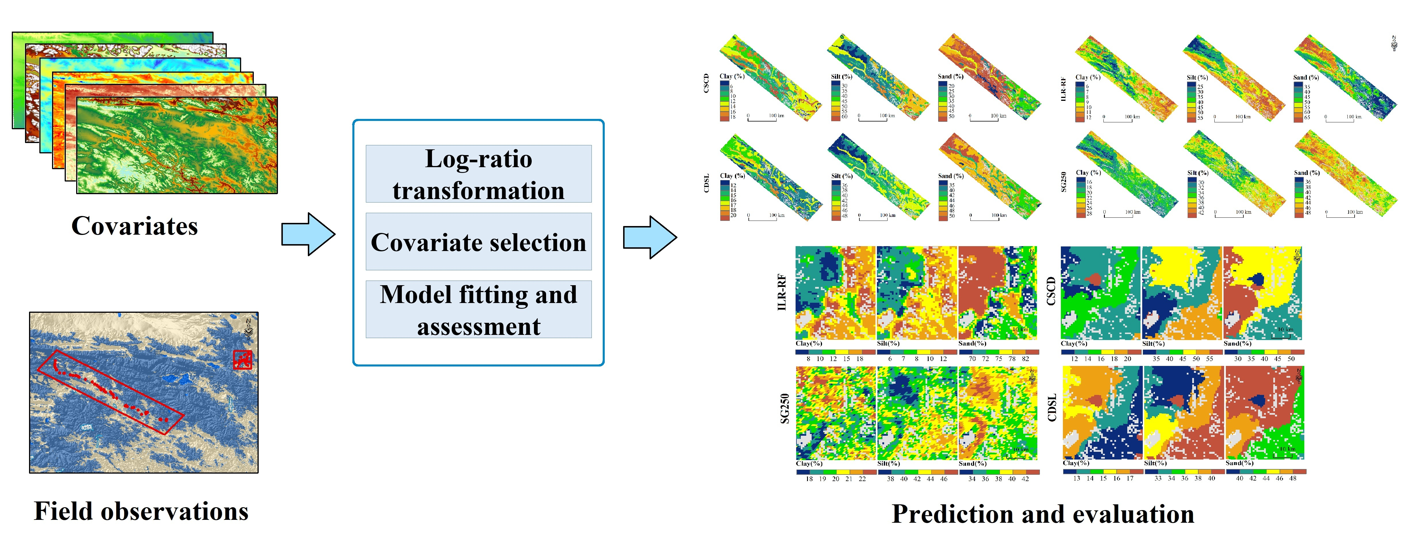
2. Materials and Methods
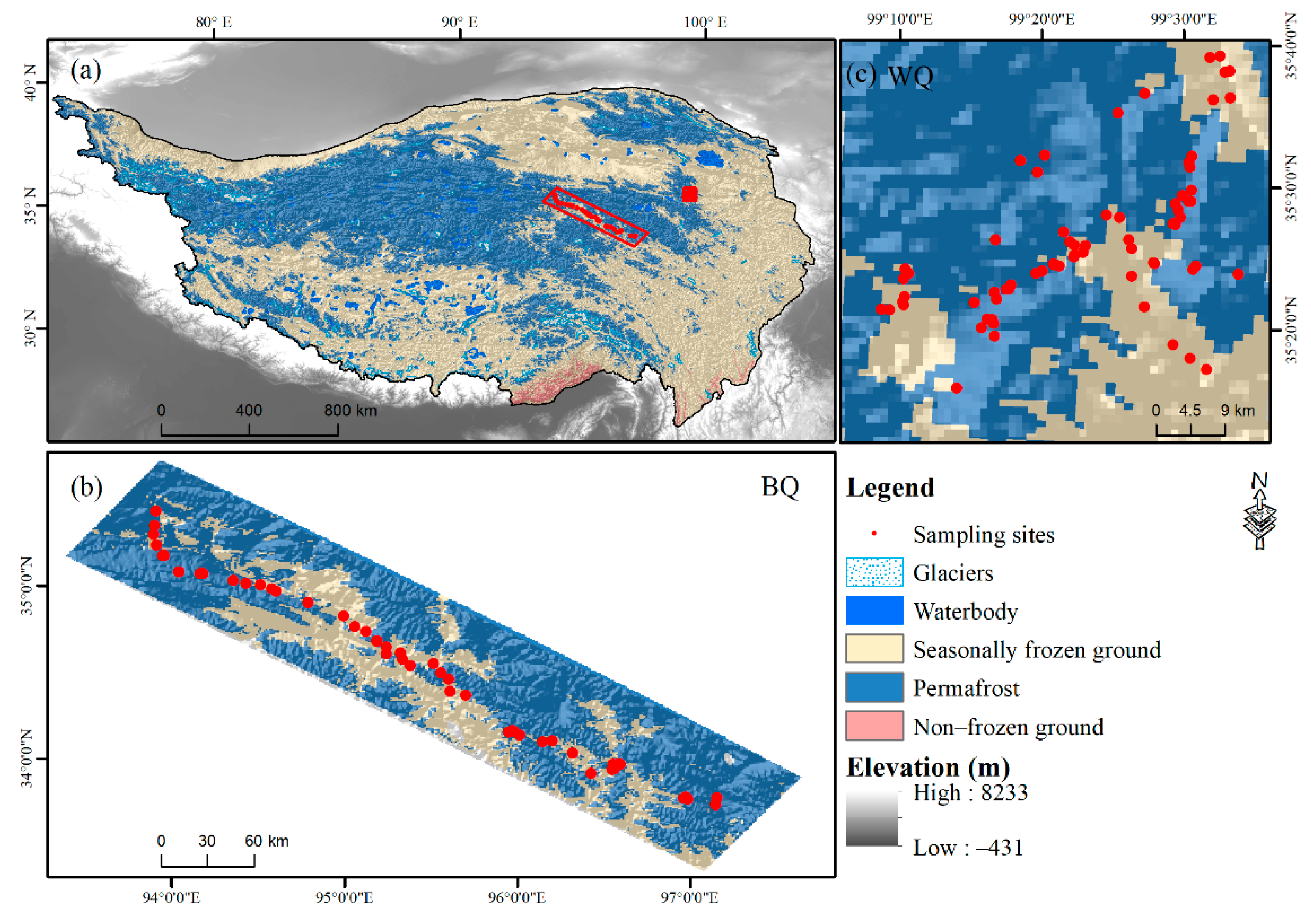
2.1. Study Area

Two typical permafrost distributed regions are selected in this study, namely Wenquan (WQ) and Budongquan-Qingshuihe (BQ) (Figure 1). WQ (35.19°–35.70°N, 99.09°–99.60°E) is a typical transitional area between permafrost and seasonally frozen ground in the northeastern part of the QTP [36,37]. It covers an area of about 2572 km2, 76% of which is covered by permafrost. The altitude varies from 3570 m to 5060 m. As a cold temperate continental climate area, it is semi-humid and semi-arid [38]. The mean annual precipitation is 500–600 mm, and the mean annual temperature is −3.2 °C. WQ is primarily a grassland ecosystem, and the dominant vegetation types are alpine meadow and alpine steppe. The parent materials are slope deposits and residual deposits [36].
BQ (33.34°~35.73°N, 93.39°~97.65°E) is located in the transition from the hills in the central to the low mountains in the eastern permafrost region [36]. The permafrost zones transit from the large extent of continuous warm and ice-rich permafrost to the alpine and mountainous isolated permafrost in the east [36,37]. It covers an area of about 31,270 km2. Its altitude varies from 3770 m to 5190 m. The annual mean air temperature is −4.4 °C, and the mean annual precipitation is 435 mm, with less precipitation from the east to the west. The climatic conditions change from the semi-arid cold in the west to the semi-humid cold regions in the east. Consequently, the primary vegetation types vary from the alpine meadow, alpine steppe to alpine desert. BQ embodies all the soil types of the permafrost region in the eastern Qinghai–Tibet Plateau, and mainly developed on the alluvial and fluvial deposit and slope deposit [36,38].

2.2. Data Sources

2.2.1. Soil Sampling

The sampling sites of the two study areas were selected with full consideration of parent material, terrain, vegetation, human activities, and accessibility. Referring to the Standard of Soil Profile Description (created by the Institute of Soil Science, Chinese Academy of Sciences) and the Field Book for Describing and Sampling Soils [39], all the soil profiles have been well documented [36]. A total of 73 sites in the WQ region were visited for sampling from September to October in 2009 and 55 sites in the BQ region from July to August in 2011. Samples were air-dried and then passed through a 2 mm sieve. After averaging the samples that share the same covariate value, 59 samples and 49 samples were left for the WQ and BQ region, respectively. Since environmental covariates have more intense impact on the topsoil than the deep soil [40], this study focused on the soil PSFs of surficial horizon (0–30 cm). The sand (particles 2000–50 μm), silt (particles 50–2 μm), and clay (particles < 2 μm) contents were determined using the pipette method [41] for samples from the WQ region and samples from BQ were analyzed by laser diffraction (LS13320, Beckman Coulter Inc., Brea, CA, USA).

2.2.2. The Environmental Covariates

In this study, we used a total of 160 covariates to represent environmental conditions (Table 1). The climatic covariates include precipitation, air temperature, and land surface temperature (LST) over 2003–2011. The precipitation and air temperature were obtained from the national Tibetan Plateau data center [42], and LST was obtained from the MOD11A1 and MYD11A1 datasets of moderate resolution imaging spectrometer (MODIS) observations. The daytime and nighttime LST were filtered according to the quality indicators of MOD11A1 and MYD11A1 [43]. Hence, the LST difference was generated as well. The maximum, minimum, and mean of seasonal and annual daytime and nighttime LST, and its difference and mean over nine years, were calculated, as was the maximum, minimum, and mean of seasonal and annual air temperature and precipitation. The digital elevation model (DEM) data were derived from the WorldClim database [44], and the DEM derivatives were computed using SAGA GIS v2. Vegetation conditions were represented by net primary productivity (NDVI), enhanced vegetation index (EVI), and gross primary productivity (GPP), which were derived from the MOD13A3, MYD13A3, MOD17A2H, and MYD17A2H datasets over nine years [43]. The annual NDVI, EVI, and GPP were processed by the maximum value composite approach. The vegetation and climate covariates in the sampling year and the multiyear average were extracted to the sampling sites. All the covariate layers were projected to the Albers conic equal area projection and resampled to 1 km by the bilinear method. Besides, a land cover classification dataset, namely the dataset of land cover in Northwest China from 1990 to 2010 [45], was used to mask out water bodies, residential areas, pavement, bare rock, snow cover, and glaciers.

2.2.3. Existing Datasets of Soil PSFs

Three existing PSF datasets were applied in comparison with our prediction. A China soil characteristic dataset (CSCD) [46] was developed by the polygon linkage method based on 8595 soil profiles and the soil map of China. The content of clay and sand was captured by two layers with a spatial resolution of 30 arc seconds (~1 km). In this study, the clay and sand content in the top horizon (0–30 cm) was used. A China dataset of soil properties for land surface modeling (CDSL) [10] was developed for the application in land surface modeling by the polygon linkage method as well. The vertical variation of each soil property was captured by eight layers, and the soil fractions of the top four vertical layers (i.e., 0–0.045, 0.045–0.091, 0.091–0.166, 0.166–0.289 m) were used in this study. The SoilGrids250m dataset (SG250) was developed by ensemble machine learning approaches with 150,000 sites spread over all continents [8]. It generated soil attributes at seven standard depths with a spatial resolution of 250 m, and the uppermost layers (0, 5, 15, and 30 cm depths) were generalized using Equation (1) in this study.

2.3. Compositional Data and Transformation

2.3.1. Conversion of PSFs in the Surface Layer

The original soil PSFs were recorded along genetic horizons in the United States Department of Agriculture (USDA) soil taxonomy. The PSFs from 0 to 30 cm depths were generalized using the following:
f ( x ) = i = 1 n 1 30 x i d i
where f(x) is a soil PSF (i.e., clay, silt, or sand) at the depth of 0–30 cm, xi is the soil PSF of the ith horizon, and di is the depth of the ith horizon. The PSFs conversion of the CDSL and SoilGrids250m datasets followed the same rule.

2.3.2. Transformation of Compositional Data

Former studies have evaluated the performance of four commonly used log-ratio transformations. The additive log-ratio (ALR) transformation [12] was the most classic and widely used, but arbitrarily choosing the divisor in ALR transformation may result in problems in compositional data analysis. To solve the problems of ALR transformation, isometric log-ratio (ILR) transformation [15] was proposed, and ILR has been evaluated with satisfactory performance in soil PSF mapping [1,15]. Therefore, in this study, ALR and ILR transformations were employed. The ALR transformation is defined as:
A L R ( x i ) = ln x i x D ,   i = 1 ,   2 ,   ,   D
The ALR back-transformed equation is defined as:
A L R ( x i ) ¯ = exp A L R ( x i ) i = 1 D exp A L R ( x i )
The ILR transformation [15] is defined as:
I L R ( x i ) = i i + 1 ln j = 1 i x j i x i + 1 ,   i = 1 ,   2 ,   ,   D 1
and its back-transformed equation [47] is defined as:
Y ( x i ) = j = i D I L R ( x j ) j ( j + 1 ) i 1 i I L R ( x i 1 )
where ILR(x0) = ILR(xD) = 0 and i = 1, 2, …, D, which is then back-transformed to the original soil PSFs via the following equation:
I L R ( x i ) ¯ = exp Y ( x i ) i = 1 D exp Y ( x i )
where xi represents the content of the soil PSFs. ALR(xi) and ILR(xi) represent the transformed values at the sampling site i. A L R ( x i ) ¯ and I L R ( x i ) ¯ represent the back-transformed PSFs, and D represents the dimension. The ALR and ILR functions were implemented with compositions package [48] in R 3.6.3 (R Development Core Team, 2020). The predictive results were back-transformed to three soil PSFs (i.e., clay, silt, and sand) using alrInv and ilrInv functions.

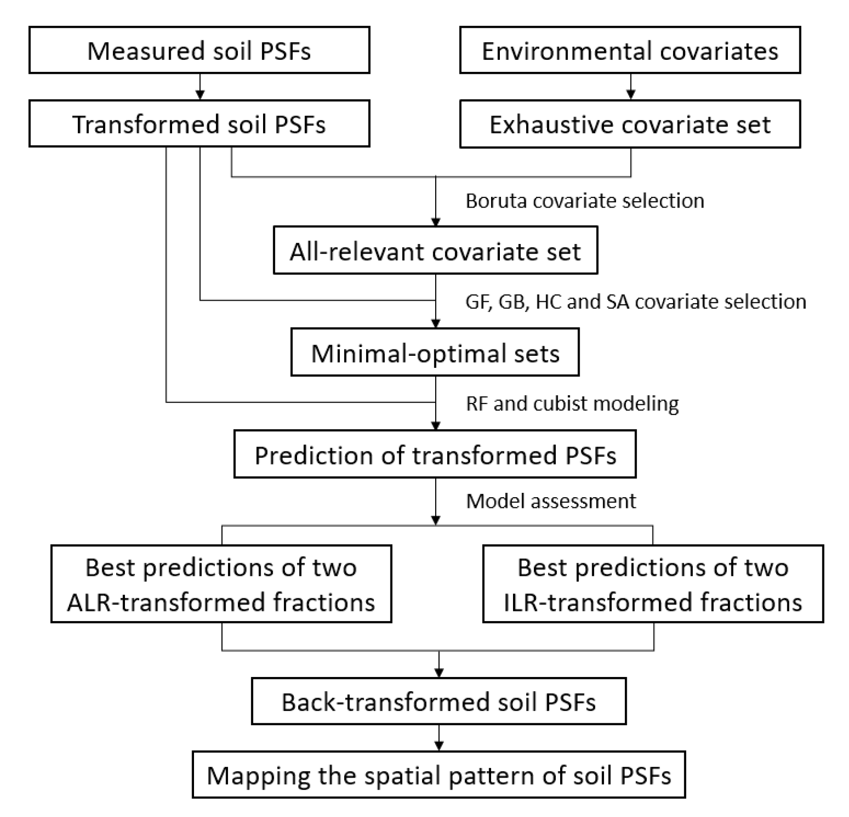
2.4. Covariate Selection Techniques

The Boruta method was applied to sort out all-relevant covariates for soil PSFs prediction. It is a wrapper method, developed on the basis of random forest (RF) algorithm. Therefore, similarly to RF, it can handle nonlinear as well as linear relationships [21,29]. To identify the irrelevant variables, the shadow attributes are created, and their importance is used to identify irrelevant variables [29,49]. Minimal-optimal features were selected to develop parsimonious models for PSF prediction. Instead of exhaustively searching all possible subsets of all relevant sets, which are computationally intensive and impractical, strategic subset selection techniques suggested by Xiong et al. [21] were employed. In this study, greedy forward (GF), greedy backward (GB), hill climbing (HC), and simulated annealing (SA) were implemented to compose the minimal-optimal sets [50]. The greedy algorithms, including GF, GB, and HC, search for local optima. The GF algorithm starts evaluating subsets with only one predictor variable. Then, by adding predictor variables one by one, GF finds its best subset. On the contrary, the GB algorithm begins with the whole set and drops predicting variables in turn until it finds its best subset. HC algorithm starts with a subset composed of arbitrarily selected variables. It finds a better subset by incrementally including or eliminating one variable only when a subset has higher predictive power. SA is a heuristic algorithm searching for global optima. It resembles the annealing procedure in metallurgy and starts from a certain higher “temperature” (i.e., initial temperature) to find the optima [51,52]. As the temperature decreases at a certain rate, the optima in the algorithm gradually stabilizes, but this may be a local optimum rather than a global one. To find the global optima, SA introduces a random update to a subset, making it possible to accept a worse prediction to escape local optima and reach the global optima [50]. These four covariate selection algorithms were implemented with Boruta [29], rpart [53], caret [54], and Fselector [55] packages in the R statistical Programming Language.

2.5. Development and Assessment of Predictive Models

On the basis of exhaustive and selected covariate sets, two log-ratio transformations (i.e., ALR and ILR) were combined with random forest (RF) and Cubist, consisting of four models (i.e., ALR-RF, ILR-RF, ALR-Cubist, and ILR-Cubist) for soil PSFs prediction (Figure 2). RF is currently the most widely used machine learning approach in Digital Soil Mapping (DSM) [19,24]. It is an ensemble learning algorithm that improves its accuracy and robustness by combining the predictions of a random population of regression trees [17,21,56]. At each split, it randomly selects predictor variables to grow trees, while on the tree level, it randomly selects samples from the training set [56]. Cubist has recently increased in popularity in DSM [18]. Cubist is a rule-based regression technique that builds multivariate linear regression models at the terminus of a tree [57]. At the terminal node of a given tree, the final model shows a collection of machine learning regression models for calculating predicted values [24]. RF and Cubist were implemented with randomForest [58] and Cubist [59] packages in the R environment. The prediction of transformed and back-transformed soil PSFs was assessed by the 10-fold cross-validation and evaluated using the coefficient of determination (R2), Root Mean Square Error (RMSE), and bias. Bias was calculated as the observed mean minus the predicted mean. The others were calculated as follows:
R 2 = i = 1 n ( x i x i ¯ ) 2 ( x i x i ¯ ) 2
R M S E = 1 n i = 1 n ( x i x i ) 2
where xi represents the observed PSF, xi′ is the simulated PSF, x i ¯ is the mean of xi, and n represents the sample size. R2 and RMSE are used to measure the data dispersion and reflect the difference between the predictions and the observations. Bias can be used to detect the over fitting of the predictive models.

3. Results

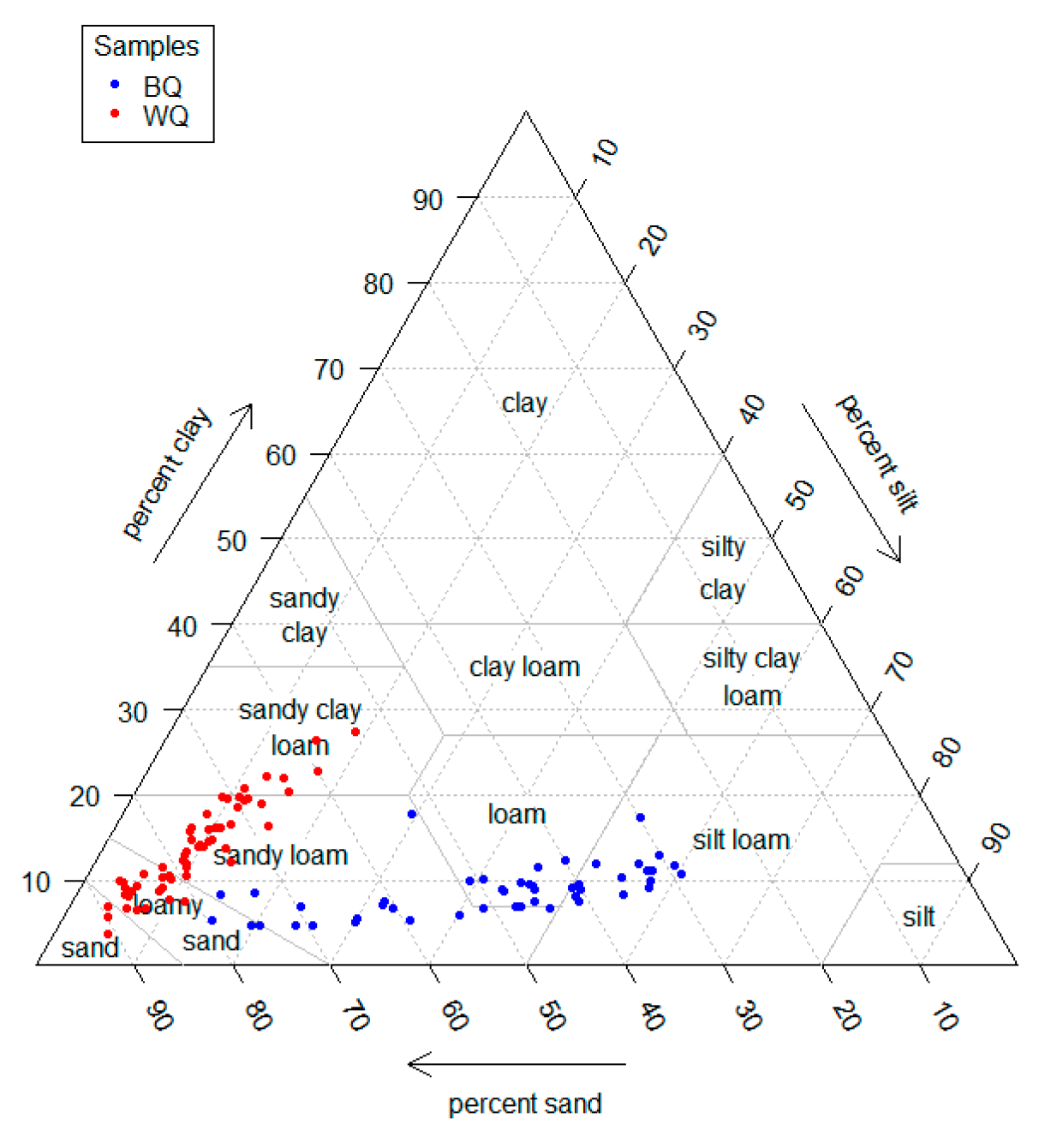
3.1. Descriptive Statistics of Observations

Surface soil textures across the BQ region are mainly sandy loam, loam, and silt loam, with a few samples of loamy sand (Figure 3). While across the WQ region dominant surface soil textures are loamy sand and sandy loam, and a few samples of sand and sandy clay loam are less dominant (Figure 3). Table 2 provides descriptive statistics for both regions; the average clay content (8.8%) at the BQ region is much less than silt (42.0%) and sand (49.2%), and sand is the most variable fraction (SD = 14.9%). Meanwhile, in the WQ region, sand content (76.5%) is much higher than that of clay (14.0%) and silt (9.5%), with the most significant variation (SD = 8.7%). The sand content of WQ was much higher, and the soil texture is coarser than that of BQ.

3.2. Covariate Sets

3.2.1. All-Relevant Variable Set

In the BQ region, the Boruta technique retained a series of vegetation, LST (land surface temperature), and precipitation covariates, composing the all-relevant (AR) set of clayalr (Figure S1). The s2_dn_e_1 (the diurnal LST in summer of the sampling year) was the most relevant covariate to explain the clayalr variation. The AR set of siltalr was composed of a series of vegetation, terrain, LST, and precipitation covariates, in which the NDVI_9 was the most relevant covariate. In terms of the ILR-transformed fractions, the AR set for clayilr prediction composed of vegetation, terrain, LST, and precipitation covariates (Figure S1). Slope (Slp) was the most relevant covariate. Whereas for siltilr, the s2_dn_e_1 was the most relevant covariate. None of the topographic covariates was relevant to ILR-transformed fractions. Moreover, the air temperature was not relevant to neither of the transformed PSFs in this region.
In the WQ region, vegetation and LST covariates were retained in AR sets to infer the variance of ALR- and ILR- transformed PSFs (Figure S2). The GPP_1 and s4_n_i_9 showed the most robust relevance to clayalr and siltalr, respectively. The s4_df_e_1 and GPP_1 were the most relevant covariates of clayilr and siltilr, respectively (Figure S2).
In this study, the common covariate categories selected in both study areas were vegetation and LST. The AR sets contained terrain and precipitation covariates in the BQ region but not in the WQ region. The difference of all-relevant covariate sets probably indicated the difference in the formation of soil PSFs in two study areas.

3.2.2. Minimal-Optimal Variable Set

In both study areas, the GB (greedy backward) sets were composed of similar covariates as AR sets to predict ALR- and ILR-transformed fractions. For the clayalr in the BQ region, HC excluded annual and winter LST on the basis of the AR set, SA (simulated annealing) further excluded vegetation covariates, and GF (greedy forward) merely retained three summer LST covariates. In terms of siltalr, HC (hill climbing) excluded terrain covariates, SA further excluded spring LST, and GF merely retained a vegetation covariate, two spring LSTs, and a precipitation covariate. For the prediction of clayilr, HC excluded annual LST, SA excluded summer LST, winter LST, and precipitation, and GF merely retained a topographical covariate and a winter LST. Meanwhile, for siltilr modeling, compared with the AR set, the SA technique excluded vegetation covariates, HC further excluded annual LST, and GF merely retained a vegetation covariate and a summer covariate (Table S1).
In the WQ region, based on the AR set of clayalr, HC excluded annual LST, SA excluded vegetation covariates, and autumn LST, while GF retained a winter LST covariate and an annual LST covariate. For the siltalr prediction, SA excluded autumn LST, HC further excluded vegetation covariates and annual LST, while GF retained an annual LST and two winter covariates. In terms of ILR-transformed fractions, HC excluded spring and annual LST for clayilr prediction, SA further excluded summer LST, and GF retained two biotic covariates, and one spring LST covariate. For the siltilr, HC excluded spring, autumn, and annual LST covariates, SA excluded spring, summer, annual LST covariates, and GF excluded vegetation and spring LST covariates (Table S1).

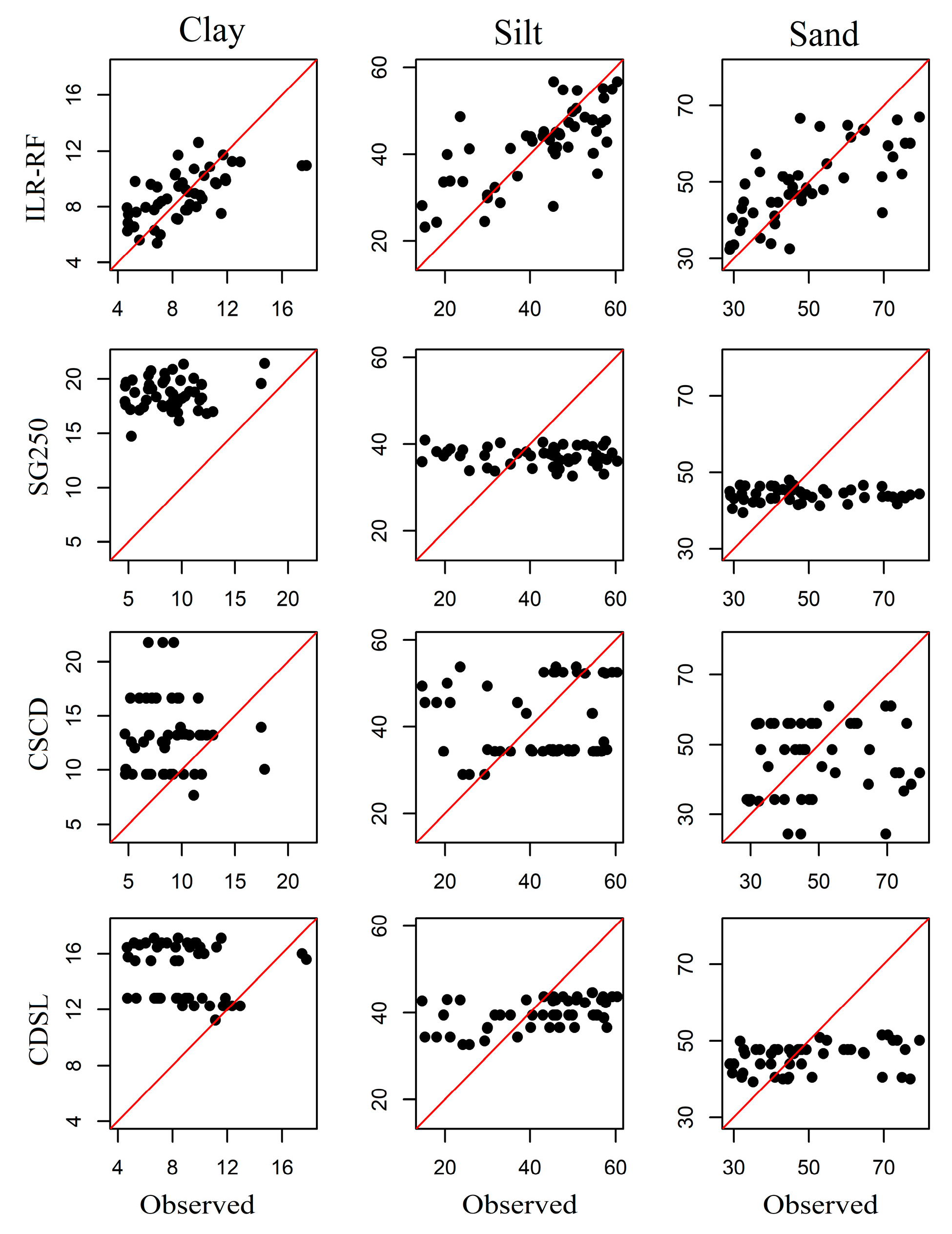
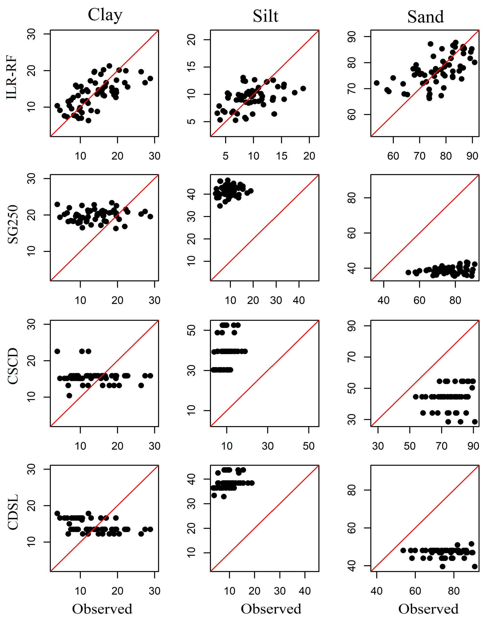
3.3. Assessment of Model Performance

According to the 10-fold cross-validation of the two ALR-transformed PSFs in the BQ region (Table S2), the RF (random forest) predictions based on AR (all-relevant variable) sets were better than the AV (exhaustive covariate) sets, and the best prediction of the two ALR-transformed PSFs were both based on the HC (hill climbing) sets. Meanwhile, for the predictions by Cubist, the AR sets performed better than AV sets for the prediction of siltilr and worse for the prediction of clayilr. As for the predictions with minimal-optimal variable sets, SA (simulated annealing) set had the best prediction on clayalr, and GB (greedy backward) set had the best prediction on siltalr. Both of them were better than the prediction based on AV and AR sets. As for the back-transformed PSFs, the ALR-RF model performed better than ALR-Cubist. According to the predictions by ILR-RF, the AR sets performed better than the AV sets. Among the minimal-optimal variable sets, SA and HC sets performed best on the prediction of clayilr and siltilr, respectively. As for the predictions by Cubist, AR set performed better than AV set on clayilr and worse on siltilr. Among the minimal-optimal variable sets, SA sets had the best predictions of both components. The ILR-RF model exhibited superior prediction compared to all the other predictions in the BQ region.
In the WQ region, AR sets outperformed AV sets by ALR-RF. Among the minimal-optimal variable sets, SA and HC sets had the best prediction on clayalr and siltalr, respectively, which were better than AR sets. As for the predictions by ALR-Cubist, AV sets outperformed AR sets. GB and HC sets had the best prediction on clayalr and siltalr, respectively, which were better than AV sets. According to the back-transformed PSFs, ALR-Cubist outperformed ALR-RF. According to the prediction of transformed PSFs by ILR-RF, AR sets performed better than AV sets. Among the minimal-optimal variable sets, GB and GF sets had the best prediction on clayilr and siltilr, respectively, better than AR sets. When using ILR-Cubist, AR sets performed better than AV set. Among the minimal-optimal sets, GF and SA sets had the best prediction on clayilr and siltilr, respectively, better than the AR sets, and outperformed all the other predicted soil PSFs in the WQ region (Table S2).
The model assessment on back-transformed PSFs was presented in Table 3. In terms of RMSE, RF (random forest) performed better than Cubist, and ILR transformation performed better than ALR in general. The prediction by ILR-RF was best in both study areas. For the prediction of clayilr at the BQ region, SA retained vegetation (i.e., evi_1, evi_9, ndvi_1, and gpp_9), terrain (i.e., SWI and VRM), and LST (i.e., yr_n_i_9) covariates. In terms of the siltilr prediction, HC retained terrain (i.e., s1_d_a_1, s2_df_a_9, s2_df_a_1 and s3_d_a_9) and climatic (i.e., pre_s1_9) factors. The SA and HC set covered all categories of covariates contained in AR sets of ILR-transformed PSFs. In the WQ region, GB retained vegetation (i.e., evi_1, evi_9, ndvi_1 and gpp_9) and LST (i.e., s1_d_i_9, s1_n_i_9, s2_d_e_1, s2_df_e_1 and s4_df_e_9) covariates for clayilr prediction. Furthermore, GF only retained LST covariates (i.e., s2_df_a_1, s3_df_i_9, s4_d_e_9, s4_n_e_1, s4_n_i_9 and yr_n_i_9) for siltilr modeling. The GB and GF sets contained all types of all-relevant covariates as well.
Predictions based on five covariate sets were different, even using the same prediction model. In general, all-relevant models had comparable performance to exhaustive models across all four prediction methods, indicating that the AR sets contained almost equivalent predictive power to exhaustive variables. Including the irrelevant variables in the exhaustive models resulted in essentially similar model accuracy but dramatically increased model complexity. Furthermore, compared with predictions on the AV or AR set, minimal optimization techniques helped improve the model performance (Table S2), even though the specific subset searching strategies were different in modeling methods and study areas. The improved predictive accuracy on the basis of minimal-optimal sets indicates that minimal optimization techniques can further decrease data redundancy on the basis of AR set. Furthermore, redundant variable information may interfere with the learning process, thereby reducing the prediction accuracy. Hence, covariate selection should be prior to model fitting in soil PSFs prediction.

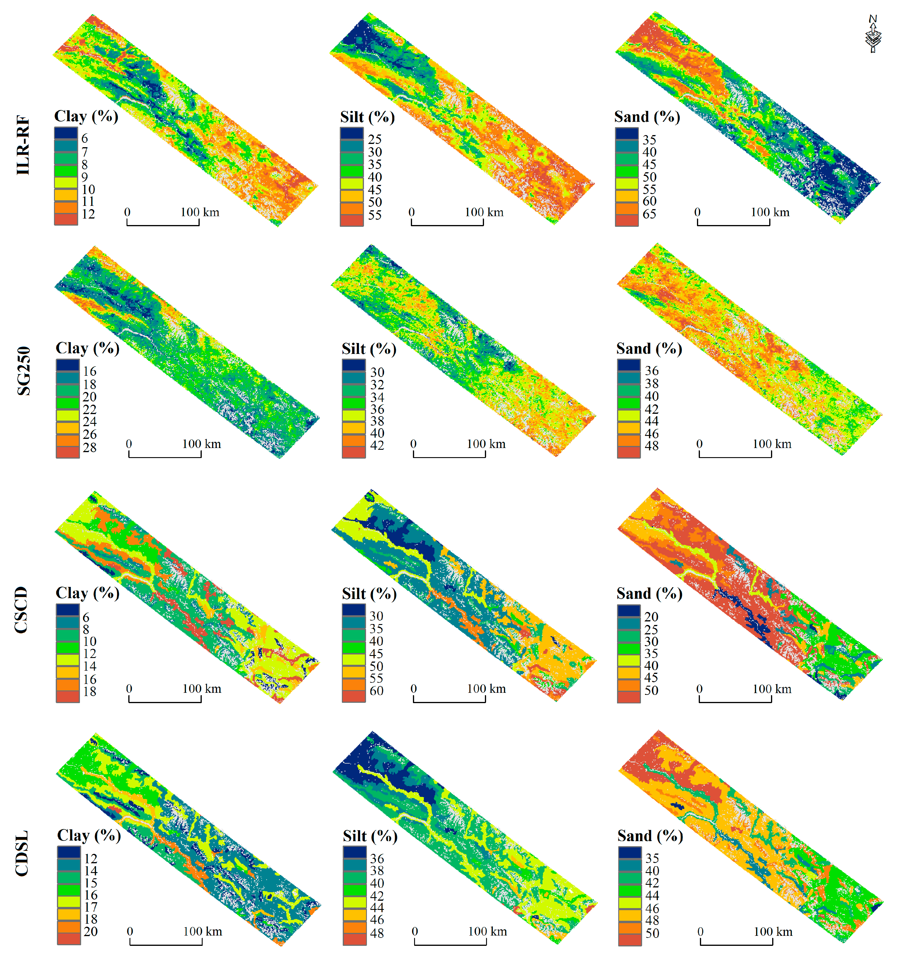
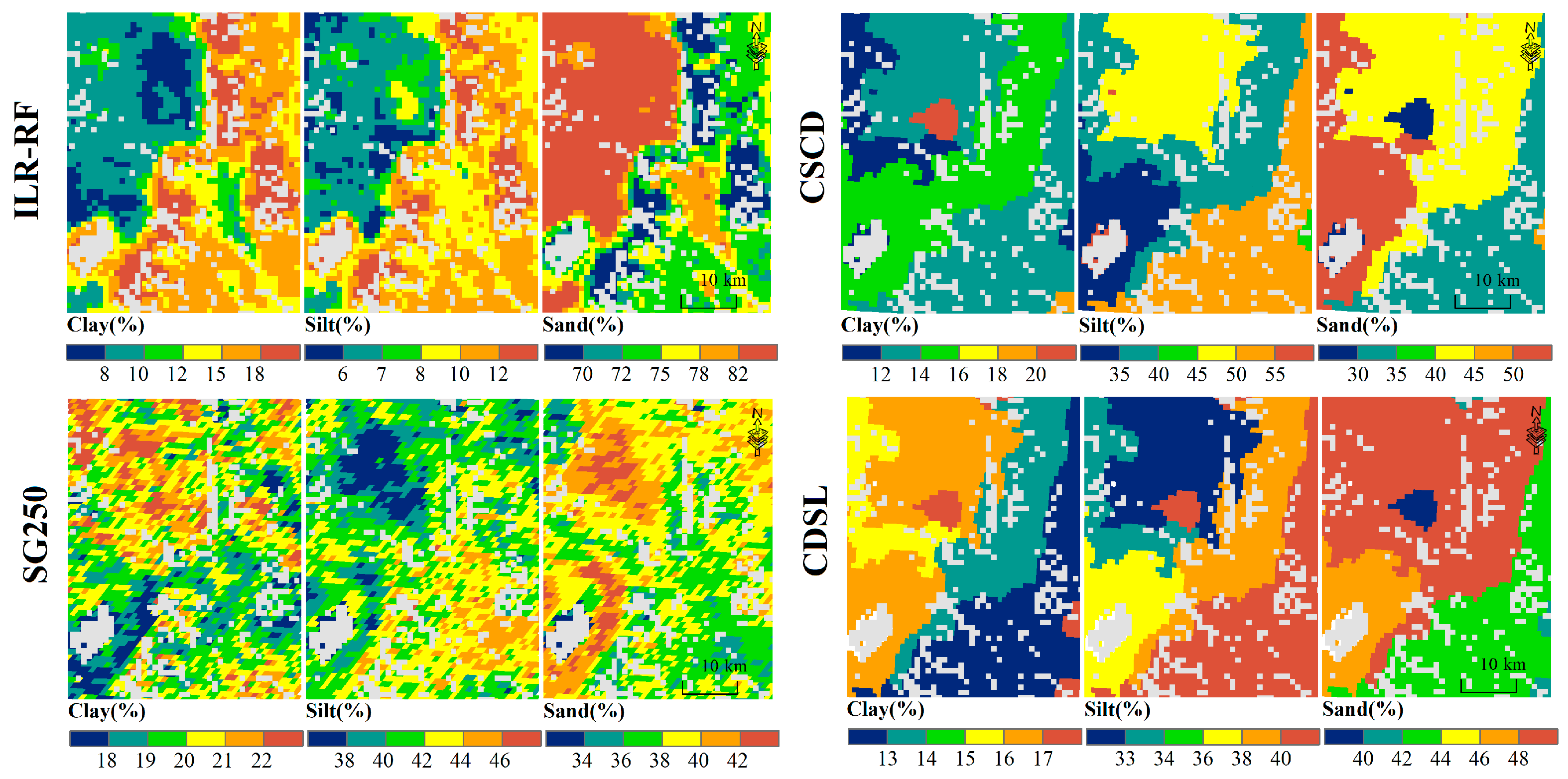
3.4. Spatial Distribution of the Predicted Soil PSFs

Even though ALR and ILR models were developed on the basis of different covariate sets, they included the same categories of covariates, and the log-ratio models generated similar spatial patterns of soil PSFs (Figures S3 and S4). Higher clay and silt content were mainly distributed in the eastern part in the BQ region, while higher sand content was mainly distributed in the northwestern part. Soil PSFs showed a similar distribution trend at the WQ region, where higher clay and silt and lower sand content distributed in the southeastern part.

4. Discussion

4.1. Covariates Most Relevant to Soil PSF Mapping

The covariate collection relies on a priori knowledge so that the explicit covariate exhaustive sets are often unlike [21,26]. Their selection determines the soil mapping performance to a great extent, especially when the number of soil samples is limited, but soil spatial heterogeneity is high [25]. The strategy of this study was to collect environmental covariates as comprehensively as possible, and the selection of key covariates was achieved by covariates reduction techniques.
AR (all-relevant covariate) sets were used to reveal the underlying process of soil–environment systems of interest [21]. Although the specific covariates retained were differential among AR sets in this study, the Boruta technique retained vegetation and LST (land surface temperature) covariates in both BQ and WQ regions. This indicated that vegetation and LST covariates are the key covariates to identify the spatial variance of soil PSFs of the surface layer. LST is the crucial indicator for the distribution of permafrost [37], and vegetation has an interactive influence on the active layer [60]. Permafrost degradation on the QTP is in company with the shift in vegetation types and species composition [61,62], decrease in vegetation biomass, productivity, and species abundance [60,63,64]. Under a warming climate, degrading permafrost has profoundly and extensively affected alpine ecology [60]. With the degradation of alpine ecosystem, the soil nutrient declined and surface soil texture became rough [30,64].
With different search techniques, minimal-optimal sets were composed of different covariates. It is because the covariates selected by local optimization methods (i.e., GB, GF, and HC) depend on the initial set that the algorithm starts searching with. In general, each data reduction technique has its advantages. For instance, the GF models are the simplest with the least variable redundancy, while GB models retain the most variable information, reflecting more processes [21]. However, they all have their disadvantages as well. The GF models only reflect the major processes and often fell short in model performance. The SA algorithm escapes the local optima by accepting some models that have been degraded due to including or excluding additional sets of variables [52,65]. In this study, the selected covariates in minimal-optimal sets were different for modeling ALR- and ILR-transformed PSFs. However, they all involved all categories of relevant covariates. For example, in the BQ region, topographic factors were relevant for ALR- and ILR-transformed PSFs. None was retained to predict clayalr, while one topographic factor was retained to predict siltlalr. Topographic factors were also selected for clayilr prediction while excluded for siltilr prediction.
Former studies also emphasized the covariate selection in digital soil mapping, indicating covariate selection can help improve model performance [25,26]. However, we cannot explicitly assign a universal covariate reduction method for soil PSFs prediction because the predictions based on selected covariates can differ in PSF transformations, modeling techniques, and study areas. It is also the reason why we did not inverse the prediction of transformed PSFs on the basis of the same selection strategy. We prefer to apply and compare multiple covariate selection strategies for each transformed soil fraction based on our results.

4.2. Prediction Models

Considering the compositional nature of soil PSFs, we applied ALR (additive log-ratio) and ILR (isometric log-ratio) transformations before model fitting in this study. Some studies also reported application of the log-ratio transformations coupled with machine learning approaches. For example, Wang et al. [17] implemented the ALR and ILR transformation with the boosted regression tree (BRT), RF, and regression kriging for a river basin. The results indicated that machine learning approaches improved the mapping performance rather than regression kriging, and the ILR-RF model outperformed the ILR-BRT model. However, Amirian-Chakan et al. [1] cast doubts on the necessity of using log-ratio transformations in soil PSFs prediction. They predicted transformed and untransformed PSFs by RF and applied the predictions to estimate available soil water capacity (AWC) and the total amount of irrigation water (TIW). The results indicated no apparent difference in the prediction of PSFs, AWC, and TIW. Moreover, they suggested that the log-transformations may lead to biased estimation of PSFs, and the bias can further propagate to pedo-transfer functions. Therefore, they believed the untransformed PSFs were still valid for predicting AWC (or TIW). Some other studies may also support this concept, for they applied Digital Soil Mapping (DSM) without log-ratio transformations in soil PSFs mapping but gained fairly good accuracy [8,22]. More studies are still needed to testify to the rationality and the feasibility of log-ratio transformation in DSM at different scales.
Former studies used the variable importance of the RF algorithm to interpret the relation between covariates and response variables. For example, Ran et al. [5] found seven variables, including the freezing degree-days, thawing degree-days, leaf area index, snow cover days, elevation, soil moisture, and soil bulk density, are selected to estimate the mean annual ground temperature. The relative importance results in Wang et al. [17] showed that soil organic carbon, NDVI, elevation, precipitation, and temperature were the main predictors to explain the variability of transformed PSFs in the Heihe River basin (area = 14.67 × 10⁵ km2). According to the study [1] at a region in southwestern Iran (area = 4600 ha), the relative importance showed that MRVBF, NDVI, elevation, slope, and band 3 of Landsat 8 were the significant covariates in predicting clay, silt, and sand when using terrain attributes and optical images. While on a larger spatial scale, Akpa et al. [66] indicated that climatic elements (precipitation and temperature), Landsat8 bands (band 2 and 3), elevation, and geology were the most influential predictors for the distribution of clay and sand in Nigeria. Liu et al. [22] found that climatic elements (e.g., solar radiation, wind speed, temperature seasonality, daytime LST), altitude, and regolith thickness were the essential factors in predicting soil PSFs in China. Hengl et al. [8] illustrated that depth, climatic elements (precipitation, precipitable Water Vapor images, daytime, and nighttime LST), and terrain factors were the most influential covariates. For soil PSFs prediction, vegetation condition is more influential on a regional scale than a national or global scale. Climatic elements are more critical on a large spatial scale, such as national and global scales.
In this study, variable importance by the parsimonious ILR-RF models at both the BQ and WQ regions were given in Figures S5 and S6. The variable importance in RF algorithm was given with two aspects. One is the mean decrease in accuracy and the other is the mean decrease in Gini index when a particular predictor variable is removed [58]. The VRM (Vector Ruggedness Measure) and s2_df_a_9 (multiyear average of maximum diurnal LST difference in summer) were the most important covariates for clayilr and siltilr prediction in the BQ region, respectively (Figure S5). In the WQ region, s4_df_e_9 (multiyear average of mean diurnal LST difference in winter) and yr_n_i_9 (multiyear average of annual minimum night LST) were the most influential covariates. Compared with the BQ region, the winter LST seemed to have a more substantial impact on soil PSFs prediction at the WQ region since a total of four winter LST covariates were used in the ILR-RF models. The vegetation (i.e., EVI, NDVI, and GPP) and LST (i.e., yr_n_i_9 and s2_df_a_1/9) covariates are the common predictors used in ILR-RF models at both regions, indicating vegetation and LST were crucial in predicting soil PSFs of the surface layer at both study areas.
Many studies found that using machine learning methods can generate soil maps with higher accuracy and smoother transitions compared with polygon linkage approach [22,63]. Nevertheless, Wadoux et al. [19] indicated that most studies emphasized the prediction and accuracy of the predicted maps for applications, while few studies accounted for existing soil knowledge in the modeling process or quantified the uncertainty of the predicted maps. Current research still falls short in revealing the underlying mechanism and the internal relationships between the soil properties and potential covariates [19,26]. Some studies found that even irrelevant predictors, i.e., pseudo predictors, can generate reasonably accurate evaluation statistics of target properties [67,68]. Behrens et al. [69,70] attributed the reason to scale and information content and proposed the “information horizon” for the interpretability of spatial environmental predictors. Besides, pedogenetic knowledge is still crucial as the key step in DSM [25,26]. However, it is hard for non-expert users to assess the feasibility of a large number of potential covariates [26]. With this respect, Qin et al. [71] and Peng et al. [26] suggested to acquire reference from the formalized covariate selection knowledge in existing applications and applied those covariates into studies of their own. For future developments, machine learning could incorporate three core elements: Plausibility, interpretability, and explainability, which will trigger soil scientists to couple model predictions with pedological explanation and understanding of the underlying soil processes [19]. Expert knowledge can be incorporated into DSM, but DSM can also lead to the discovery of knowledge [26,72]. The combination of data-driven and knowledge-based methods can promote even more significant interactions between pedology and DSM [72].

4.3. Spatial Distribution

The predicted soil PSFs showed a similar distribution trend in both study areas. The finer soil texture was distributed in the southeast or east, while the coarse soil texture was distributed in the northwest. We compared the spatial distribution of soil fractions (take sand content for example) and some of the important predictors for both regions (Figures S7 and S8) to test if the predicted PSF distribution followed the same spatial pattern as the corresponding important predictors. Since the predicted silt and clay had a similar distribution pattern, though sand was opposite, we took sand fraction as a representative. We found that in the BQ region, even though VRM had the highest variable importance in predicting clayilr, its spatial distribution was not that similar to sand. The most important predictor of siltilr, s2_df_a_9, had a very similar spatial distribution as the sand fraction in the northwest part. However, it did not depict the spatial variance of the sand fraction in the southeastern part. In contrast, some other predictors, such as EVI_1, s1_d_a_1, and s3_d_a_9, showed more a similar spatial distribution as the sand fraction. According to the land use type (Figure S7), coarse soil texture was usually distributed in the alpine desert grassland, where the elevation was relatively low, and the daytime LST (i.e., s3_d_a_9) and the LST difference (i.e., s2_df_a_9) were relatively high. The finer soil texture was usually distributed in the alpine meadow and alpine steppe. While in the WQ region, the s4_df_e_9 and yr_n_i_9 showed a similar spatial distribution pattern as the sand fraction, especially in the northwest part. The coarse soil texture was mainly distributed in the northwest WQ (Figure S8), dominated by alpine steppe and alpine desert grassland. In the northwest WQ, the minimum LST was lower, and the LST difference was larger. It indicated that the predicted distributions of soil PSFs were determined by the compound impact of multiple predictors rather than solely impacted by the most influential predictor.

4.4. Comparison with Existing Maps

Former studies have offered soil texture information at multiple spatial scales [8,22,46,73,74,75]. However, due to the lack of field observations, the availability of these datasets in permafrost areas was difficult to evaluate. The PSFs were extracted from three available datasets (Section 2.2.3), and their descriptive statistics indicated that the silt and sand content at BQ and WQ were comparable (Table 4). While the descriptive statistics of observations indicated the silt content at BQ and WQ was quite different (Table 2). Hence, the three legacy datasets failed in depicting the spatial variance of soil PSFs, especially the higher content of sand in the WQ region.
The scatter plots (Figure 4) show that the SoilGrids250m, CSCD, and CDSL overestimated the clay content and cannot capture the silt and sand variance in BQ. Besides, all three compared datasets overestimated silt fraction and underestimated sand fraction in WQ (Figure 5). They could not capture the variance of clay either.
According to the spatial distribution of soil PSFs in this study, the clay and silt content increased from northwest to the southeast in both BQ and WQ (Figure 6 and Figure 7). We notice that the CSCD and CDSL also showed a similar trend as ILR-RF prediction at BQ, while SoilGrids250m did not (Figure 6). The spatial patterns were not that consistent with ILR-RF at WQ (Figure 7). The assessment of the three legacy datasets showed low prediction accuracy on soil PSFs (Table 5).
There are some reasons to explain the low predictive power of the three legacy datasets. Firstly, observations from permafrost regions are quite deficient. The CDSL and CSCD datasets were developed on the Chinese soil profile database, which barely included observations in the permafrost distributed region. The SoilGrids250m used this database as well. Even though some vacant areas were filled with pseudo-points by expert knowledge [8], the inadequate soil samples result in insufficient learning process in model fitting. Secondly, the methodology implemented in these soil datasets were different. The CDSL and CSCD datasets used the polygon linkage approach while SoilGrids250m and our study employed the machine learning approaches. From the perspective of the earth system model, Dai et al. [76] have reviewed global soil properties maps and compared the maps generated by polygon-linkage methods with those generated by DSM. They found that the soil datasets produced by these two methods are quite different. These datasets may not be comparable since the linkage method results in an abrupt change between the boundaries of soil polygons, while the DSM simulated the soil properties with a continuous spatial change. In that way, the DSM-derived datasets can provide a more realistic estimation of soils than those derived by linkage methods. Even so, Arrouays et al. [77,78] argued that spatial information systems for polygons and grids complement various applications of soil maps. Therefore, both are needed from local to global scales. Thirdly, the initial spatial scales and spatial resolution of the datasets are different. This study was conducted at 1 km spatial resolution in two local areas. The CDSL and CSCD were developed in mainland China with a spatial resolution of 1 km, while SoilGrids250m was developed for the global scale with a spatial resolution of 250 m. When used at a local scale, they may not be able to depict the detailed information precisely. Liu et al. [22] found that the SoilGrids250m and polygon-linkage-based maps showed lower accuracy than their predictive maps of soil PSFs in China.

5. Conclusions

Due to the lack of field observations, the datasets focused on the spatial distribution of soil PSFs in permafrost regions of the Qinghai–Tibet Plateau are still scarce. We carried out the mapping of soil PSFs at two typical permafrost distributed regions by integrating two log-ratio transformation methods, five variable selection techniques, and two learning approaches. The Boruta all-relevant technique retained vegetation and LST covariates, and excluded air temperature in both regions. The difference in variable selection in the two regions is that precipitation and topographic covariates were retained at BQ but excluded at WQ. In general, the AR models had comparable accuracy with the exhaustive models, and the parsimonious models exhibited superior prediction compared to the exhaustive covariates. It confirms the necessity of variable selection prior to model fitting. However, we did not find a universal method for covariate selection. In addition, we prefer to compare multiple variable selection techniques than recommend a specific one. The ILR-RF model outperformed all the other models in both study areas. These results suggest that the combination of log-ratio transformation, covariate selection, and machine learning approaches are feasible in mapping soil PSFs in both study areas.

Supplementary Materials

The following are available online at https://0-www-mdpi-com.brum.beds.ac.uk/article/10.3390/rs13071392/s1, Figures S1 and S2: Importance of the all-relevant covariates of ALR- and ILR-transformed PSFs in the BQ and WQ regions. Figures S3 and S4: Spatial distribution of soil particle size fractions in the BQ and WQ regions predicted by four log-ratio models. Figures S5 and S6: Fitted variable importance plots for clayilr and siltilr by the ILR-RF model in the BQ and WQ regions. Figures S7 and S8: Comparison between the distribution of sand and the predictors in the BQ and WQ regions. Table S1: Selected covariates identified by Boruta, GF, GB, HC and SA techniques in the two study areas. Table S2: Assessment on the predictions of two transformed fractions by the exhaustive, all-relevant and parsimonious models.

Author Contributions

Conceptualization, C.W. and L.Z.; methodology, C.W. and L.Z.; software, C.W., L.W., and Z.X.; validation, C.W. and D.Z.; formal analysis, H.F. and C.W.; investigation, H.F., G.H., X.W., Y.Z., Y.S., Q.P., E.D., and G.L.; resources, L.Z. and H.F.; data curation, C.W., H.F., and D.Z.; writing—original draft preparation, C.W., L.Z., and Z.X.; writing—review and editing, all co-authors; visualization, C.W., Z.X., and L.W.; supervision, L.Z.; project administration, L.Z.; funding acquisition, H.Y. All authors have read and agreed to the published version of the manuscript.

Funding

This research was funded by the Second Tibetan Plateau Scientific Expedition and Research (STEP) program (No. 2019QZKK0201), the National Natural Science Foundation of China (No. 41931180), and the opening research foundation of Key Laboratory of Frozen Soil Engineering (No. SKLFSE201921).

Institutional Review Board Statement

Not applicable.

Informed Consent Statement

Not applicable.

Data Availability Statement

Not applicable.

Acknowledgments

We thank Tian, Liming and Fan, Lei for their generous help in data processing and writing. We also thank the anonymous reviewers for their constructive comments and suggestions.

Conflicts of Interest

The authors declare no conflict of interest.

References

  1. Amirian-Chakan, A.; Minasny, B.; Taghizadeh-Mehrjardi, R.; Akbarifazli, R.; Darvishpasand, Z.; Khordehbin, S. Some practical aspects of predicting texture data in digital soil mapping. Soil Tillage Res. 2019, 194, 104289. [Google Scholar] [CrossRef]
  2. Minasny, B.; McBratney, A.B. Regression rules as a tool for predicting soil properties from infrared reflectance spectroscopy. Chemom. Intell. Lab. Syst. 2008, 94, 72–79. [Google Scholar] [CrossRef]
  3. Van Looy, K.; Bouma, J.; Herbst, M.; Koestel, J.; Minasny, B.; Mishra, U.; Montzka, C.; Nemes, A.; Pachepsky, Y.A.; Padarian, J.; et al. Pedotransfer Functions in Earth System Science: Challenges and Perspectives. Rev. Geophys. 2017, 55, 1199–1256. [Google Scholar] [CrossRef] [Green Version]
  4. Wang, X.; Xiao, J.; Li, X.; Cheng, G.; Ma, M.; Che, T.; Dai, L.; Wang, S.; Wu, J. No Consistent Evidence for Advancing or Delaying Trends in Spring Phenology on the Tibetan Plateau. J. Geophys. Res. Biogeosci. 2017, 122, 3288–3305. [Google Scholar] [CrossRef]
  5. Ran, Y.; Li, X.; Cheng, G.; Nan, Z.; Che, J.; Sheng, Y.; Wu, Q.; Jin, H.; Luo, D.; Tang, Z.; et al. Mapping the permafrost stability on the Tibetan Plateau for 2005–2015. Sci. China Earth Sci. 2020, 1–18. [Google Scholar] [CrossRef]
  6. Zhao, L.; Zou, D.; Hu, G.; Du, E.; Pang, Q.; Xiao, Y.; Li, R.; Sheng, Y.; Wu, X.; Sun, Z.; et al. Changing climate and the permafrost environment on the Qinghai–Tibet (Xizang) plateau. Permafr. Periglac. Process. 2020, 31, 396–405. [Google Scholar] [CrossRef]
  7. Sun, Z.; Zhao, L.; Hu, G.; Qiao, Y.; Du, E.; Zou, D.; Xie, C. Modeling permafrost changes on the Qinghai–Tibetan plateau from 1966 to 2100: A case study from two boreholes along the Qinghai–Tibet engineering corridor. Permafr. Periglac. Process. 2020, 31, 156–171. [Google Scholar] [CrossRef]
  8. Hengl, T.; De Jesus, J.M.; Heuvelink, G.B.M.; Gonzalez, M.R.; Kilibarda, M.; Blagotić, A.; Shangguan, W.; Wright, M.N.; Geng, X.; Bauer-Marschallinger, B.; et al. SoilGrids250m: Global gridded soil information based on machine learning. PLoS ONE 2017, 12, 1–40. [Google Scholar] [CrossRef] [PubMed] [Green Version]
  9. FAO; CAS; IIASA; ISRIC; JRC. Harmonized World Soil Database (HWSD v 1.21). Available online: https://iiasa.ac.at/web/home/research/researchPrograms/water/HWSD.html (accessed on 31 March 2021).
  10. Shangguan, W.; Dai, Y.; Liu, B.; Zhu, A.; Duan, Q.; Wu, L.; Ji, D.; Ye, A.; Yuan, H.; Zhang, Q.; et al. A China data set of soil properties for land surface modeling. J. Adv. Model. Earth Syst. 2013, 5, 212–224. [Google Scholar] [CrossRef]
  11. Odeh, I.O.A.; Todd, A.J.; Triantafilis, J. Spatial prediction of soil particle-size fractions as compositional data. Soil Sci. 2003, 168, 501–515. [Google Scholar] [CrossRef] [Green Version]
  12. Aitchison, J. The Statistical Analysis of Compositional Data. J. R. Stat. Soc. Ser. B 1982, 44, 139–177. [Google Scholar] [CrossRef]
  13. Pawlowsky, V.; Olea, R.A.; Davis, J.C. Estimation of regionalized compositions: A comparison of three methods. Math. Geol. 1995, 27, 105–127. [Google Scholar] [CrossRef]
  14. Sun, X.L.; Wu, Y.J.; Wang, H.L.; Zhao, Y.G.; Zhang, G.L. Mapping Soil Particle Size Fractions Using Compositional Kriging, Cokriging and Additive Log-ratio Cokriging in Two Case Studies. Math. Geosci. 2014, 46, 429–443. [Google Scholar] [CrossRef]
  15. Egozcue, J.J.; Pawlowsky-Glahn, V.; Mateu-Figueras, G.; Barceló-Vidal, C. Isometric Logratio Transformations for Compositional Data Analysis. Math. Geol. 2003, 35, 279–300. [Google Scholar] [CrossRef]
  16. McBratney, A.B.; De Gruijter, J.J.; Brus, D.J. Spacial prediction and mapping of continuous soil classes. Geoderma 1992, 54, 39–64. [Google Scholar] [CrossRef]
  17. Wang, Z.; Shi, W.; Zhou, W.; Li, X.; Yue, T. Comparison of additive and isometric log-ratio transformations combined with machine learning and regression kriging models for mapping soil particle size fractions. Geoderma 2020, 365, 114214. [Google Scholar] [CrossRef]
  18. McBratney, A.B.; Mendonça Santos, M.L.; Minasny, B. On digital soil mapping. Geoderma 2003, 117, 3–52. [Google Scholar] [CrossRef]
  19. Wadoux, A.M.J.C.; Minasny, B.; McBratney, A.B. Machine learning for digital soil mapping: Applications, challenges and suggested solutions. Earth-Sci. Rev. 2020, 210, 103359. [Google Scholar] [CrossRef]
  20. Minasny, B.; McBratney, A.B.; Malone, B.P.; Wheeler, I. Digital Mapping of Soil Carbon. Adv. Agron. 2013, 118, 1–47. [Google Scholar] [CrossRef]
  21. Xiong, X.; Grunwald, S.; Myers, D.B.; Kim, J.; Harris, W.G.; Comerford, N.B. Holistic environmental soil-landscape modeling of soil organic carbon. Environ. Model. Softw. 2014, 57, 202–215. [Google Scholar] [CrossRef]
  22. Liu, F.; Zhang, G.L.; Song, X.; Li, D.; Zhao, Y.; Yang, J.; Wu, H.; Yang, F. High-resolution and three-dimensional mapping of soil texture of China. Geoderma 2020, 361, 114061. [Google Scholar] [CrossRef]
  23. Li, W.; Zhao, L.; Wu, X.; Wang, S.; Sheng, Y.; Ping, C.L.; Zhao, Y.; Fang, H.; Shi, W. Soil distribution modeling using inductive learning in the eastern part of permafrost regions in Qinghai-Xizang (Tibetan) Plateau. Catena 2015, 126, 98–104. [Google Scholar] [CrossRef]
  24. Khaledian, Y.; Miller, B.A. Selecting appropriate machine learning methods for digital soil mapping. Appl. Math. Model. 2020, 81, 401–418. [Google Scholar] [CrossRef]
  25. Lu, Y.Y.; Liu, F.; Zhao, Y.G.; Song, X.D.; Zhang, G.L. An integrated method of selecting environmental covariates for predictive soil depth mapping. J. Integr. Agric. 2019, 18, 301–315. [Google Scholar] [CrossRef]
  26. Liang, P.; Qin, C.; Zhu, A.; Hou, Z.; Fan, N.; Wang, Y. A case-based method of selecting covariates for digital soil mapping. J. Integr. Agric. 2020, 19, 2127–2136. [Google Scholar] [CrossRef]
  27. Iguyon, I.; Elisseeff, A. An introduction to variable and feature selection. J. Mach. Learn. Res. 2003, 3, 1157–1182. [Google Scholar]
  28. Nilsson, R.; Peña, J.M.; Björkegren, J.; Tegnér, J. Consistent feature selection for pattern recognition in polynomial time. J. Mach. Learn. Res. 2007, 8, 589–612. [Google Scholar]
  29. Kursa, M.B.; Rudnicki, W.R. Feature Selection with the Boruta Package. J. Stat. Softw. 2010, 36, 1–13. [Google Scholar] [CrossRef] [Green Version]
  30. Yue, G.; Zhao, L.; Wang, Z.; Zhang, L.; Zou, D.; Niu, L.; Zhao, Y.; Qiao, Y. Spatial Variation in Biomass and Its Relationships to Soil Properties in the Permafrost Regions Along the Qinghai-Tibet Railway. Environ. Eng. Sci. 2017, 34, 130–137. [Google Scholar] [CrossRef]
  31. Zhao, L.; Wu, X.; Wang, Z.; Sheng, Y.; Fang, H.; Zhao, Y.; Hu, G.; Li, W.; Pang, Q.; Shi, J.; et al. Soil organic carbon and total nitrogen pools in permafrost zones of the Qinghai-Tibetan Plateau. Sci. Rep. 2018, 8, 1–9. [Google Scholar] [CrossRef]
  32. Cao, Z.; Cheng, T.; Ma, X.; Tian, Y.; Zhu, Y.; Yao, X.; Chen, Q.; Liu, S.; Guo, Z.; Zhen, Q.; et al. A new three-band spectral index for mitigating the saturation in the estimation of leaf area index in wheat. Int. J. Remote Sens. 2017, 38, 3865–3885. [Google Scholar] [CrossRef]
  33. Chen, Y.; Yang, K.; Tang, W.; Qin, J.; Zhao, L. Parameterizing soil organic carbon’s impacts on soil porosity and thermal parameters for Eastern Tibet grasslands. Sci. China Earth Sci. 2012, 55, 1001–1011. [Google Scholar] [CrossRef]
  34. Bi, H.; Ma, J.; Zheng, W.; Zeng, J. Comparison of soil moisture in GLDAS model simulations and in situ observations over the Tibetan Plateau. J. Geophys. Res. Atmos. 2016, 121, 2658–2678. [Google Scholar] [CrossRef] [Green Version]
  35. Zheng, G.; Yang, Y.; Yang, D.; Dafflon, B.; Yi, Y.; Zhang, S.; Chen, D.; Gao, B.; Wang, T.; Shi, R.; et al. Remote sensing spatiotemporal patterns of frozen soil and the environmental controls over the Tibetan Plateau during 2002–2016. Remote Sens. Environ. 2020, 247, 111927. [Google Scholar] [CrossRef]
  36. Fang, H.; Zhao, L.; Wu, X.; Zhao, Y.; Zhao, Y.; Hu, G. Soil taxonomy and distribution characteristics of the permafrost region in the Qinghai-Tibet Plateau, China. J. Mt. Sci. 2015, 12, 1448–1459. [Google Scholar] [CrossRef]
  37. Zou, D.; Zhao, L.; Sheng, Y.; Chen, J.; Hu, G.; Wu, T.; Wu, J.; Xie, C.; Wu, X.; Pang, Q.; et al. A new map of permafrost distribution on the Tibetan Plateau. Cryosph. 2017, 11, 2527–2542. [Google Scholar] [CrossRef] [Green Version]
  38. Li, W.; Zhao, L.; Wu, X.; Zhao, Y.; Fang, H.; Shi, W. Distribution of soils and landform relationships in the permafrost regions of Qinghai-Xizang (Tibetan) Plateau. Chinese Sci. Bull. 2015, 60, 2216–2226. [Google Scholar] [CrossRef]
  39. Schoeneberger, P.J.; Wysocki, D.A.; Benham, E.C.; Staff, S.S. Field Book for Describing and Sampling Soils Version 3.0; National Resources Conservation Service, National Soil Survey Center: Lincoln, NE, USA, 2012; ISBN 1782664092. [Google Scholar]
  40. Zhang, Y.; Ji, W.; Saurette, D.D.; Easher, T.H.; Li, H.; Shi, Z.; Adamchuk, V.I.; Biswas, A. Three-dimensional digital soil mapping of multiple soil properties at a field-scale using regression kriging. Geoderma 2020, 366, 114253. [Google Scholar] [CrossRef]
  41. Zhang, G.; Gong, Z. Soil Survey Laboratory Methods; Science Press: Beijing, China, 2012. [Google Scholar]
  42. Peng, S.; Ding, Y.; Liu, W.; Li, Z. 1 km monthly temperature and precipitation dataset for China from 1901 to 2017. Earth Syst. Sci. Data 2019, 11, 1931–1946. [Google Scholar] [CrossRef] [Green Version]
  43. NASA LAADS DAAC. Available online: https://ladsweb.modaps.eosdis.nasa.gov/search/ (accessed on 31 March 2021).
  44. Fick, S.E.; Hijmans, R.J. WorldClim 2: New 1-km spatial resolution climate surfaces for global land areas. Int. J. Climatol. 2017, 37, 4302–4315. [Google Scholar] [CrossRef]
  45. Yan, C.; Chang, C.; Xie, J. Land Cover Data Sets in Northwestern China from 1990 to 2010. Available online: http://www.crensed.ac.cn/portal/metadata/215ea67d-cfa5-4636-8a12-dec526332224 (accessed on 31 March 2021).
  46. Shangguan, W.; Dai, Y.; Liu, B.; Ye, A.; Yuan, H. A soil particle-size distribution dataset for regional land and climate modelling in China. Geoderma 2012, 171–172, 85–91. [Google Scholar] [CrossRef]
  47. Filzmoser, P.; Hron, K. Outlier detection for compositional data using robust methods. Math. Geosci. 2008, 40, 233–248. [Google Scholar] [CrossRef]
  48. Van den Boogaart, K.G.; Tolosana-Delgado, R. “compositions”: A unified R package to analyze compositional data. Comput. Geosci. 2008, 34, 320–338. [Google Scholar] [CrossRef]
  49. Grunwald, S. Environmental Soil-Landscape Modeling: Geographic Information Technologies and Pedometrics; CRC Press/Taylor & Francis Group: Boca Rotan, FL, USA, 2006; ISBN 0-8247-2389-9 (HB). [Google Scholar]
  50. Wehrens, R.; Wehrens, R. Variable Selection. In Chemometrics with R; Springer: Berlin/Heidelberg, Germany, 2011; pp. 205–232. [Google Scholar]
  51. Metropolis, N.; Rosenbluth, A.W.; Rosenbluth, M.N.; Teller, A.H.; Teller, E. Equation of state calculations by fast computing machines. J. Chem. Phys. 1953, 21, 1087–1092. [Google Scholar] [CrossRef] [Green Version]
  52. Lin, S.W.; Lee, Z.J.; Chen, S.C.; Tseng, T.Y. Parameter determination of support vector machine and feature selection using simulated annealing approach. Appl. Soft Comput. J. 2008, 8, 1505–1512. [Google Scholar] [CrossRef]
  53. Therneau, T.; Atkinson, B. rpart: Recursive Partitioning and Regression Trees. Available online: https://cran.r-project.org/package=rpart (accessed on 31 March 2021).
  54. Kuhn, M. Caret: Classification and Regression Training. Available online: https://cran.r-project.org/package=caret (accessed on 31 March 2021).
  55. Romanski, P.; Kotthoff, L.; Maintainer, P.S. FSelector: Selecting Attributes. R Package Version 0.31. Available online: https://cran.r-project.org/package=FSelector (accessed on 31 March 2021).
  56. Breiman, L. Random Forests. Mach. Learn. 2001, 45, 5–32. [Google Scholar] [CrossRef] [Green Version]
  57. Quinlan, J.R. C4.5: Programs for Machine Learning; Morgan Kaufmann Publishers Inc.: San Francisco, CA, USA, 1993. [Google Scholar]
  58. Liaw, A.; Wiener, M. Classification and Regression by randomForest. R News 2002, 2, 18–22. [Google Scholar]
  59. Kuhn, M.; Quinlan, R. Rule- And Instance-Based Regression Modeling. Available online: https://cran.r-project.org/web/packages/Cubist/Cubist.pdf (accessed on 31 March 2021).
  60. Jin, X.Y.; Jin, H.J.; Iwahana, G.; Marchenko, S.S.; Luo, D.L.; Li, X.Y.; Liang, S.H. Impacts of climate-induced permafrost degradation on vegetation: A review. Adv. Clim. Chang. Res. 2020. [Google Scholar] [CrossRef]
  61. Wei, S.; Cui, H.; Zhu, Y.; Lu, Z.; Pang, S.; Zhang, S.; Dong, H.; Su, X. Shifts of methanogenic communities in response to permafrost thaw results in rising methane emissions and soil property changes. Extremophiles 2018, 22, 447–459. [Google Scholar] [CrossRef]
  62. Yang, Z.P.; Gao, J.X.; Zhao, L.; Xu, X.L.; Ouyang, H. Linking thaw depth with soil moisture and plant community composition: Effects of permafrost degradation on alpine ecosystems on the Qinghai-Tibet Plateau. Plant Soil 2013, 367, 687–700. [Google Scholar] [CrossRef]
  63. Tang, L.; Dong, S.; Sherman, R.; Liu, S.; Liu, Q.; Wang, X.; Su, X.; Zhang, Y.; Li, Y.; Wu, Y.; et al. Changes in vegetation composition and plant diversity with rangeland degradation in the alpine region of Qinghai-Tibet Plateau. Rangel. J. 2015, 37, 107. [Google Scholar] [CrossRef]
  64. Guo, Z.; Niu, F.; Zhan, H.; Wu, Q. Changes of grassland ecosystem due to degradation of permafrost frozen soil in the Qinghai-Tibet Plateau. Acta Ecol. Sin. 2007, 27, 3294–3301. [Google Scholar]
  65. Sutter, J.M.; Kalivas, J.H. Comparison of Forward Selection, Backward Elimination, and Generalized Simulated Annealing for Variable Selection. Microchem. J. 1993, 47, 60–66. [Google Scholar] [CrossRef]
  66. Akpa, S.I.C.; Odeh, I.O.A.; Bishop, T.F.A.; Hartemink, A.E. Digital Mapping of Soil Particle-Size Fractions for Nigeria. Soil Sci. Soc. Am. J. 2014, 78, 1953. [Google Scholar] [CrossRef] [Green Version]
  67. Wadoux, A.M.J.C.; Samuel-Rosa, A.; Poggio, L.; Mulder, V.L. A note on knowledge discovery and machine learning in digital soil mapping. Eur. J. Soil Sci. 2020, 71, 133–136. [Google Scholar] [CrossRef]
  68. Fourcade, Y.; Besnard, A.G.; Secondi, J. Paintings predict the distribution of species, or the challenge of selecting environmental predictors and evaluation statistics. Glob. Ecol. Biogeogr. 2018, 27, 245–256. [Google Scholar] [CrossRef]
  69. Behrens, T.; Viscarra Rossel, R.A.; Kerry, R.; MacMillan, R.; Schmidt, K.; Lee, J.; Scholten, T.; Zhu, A.X. The relevant range of scales for multi-scale contextual spatial modelling. Sci. Rep. 2019, 9, 1–9. [Google Scholar] [CrossRef] [Green Version]
  70. Behrens, T.; Viscarra Rossel, R.A. On the interpretability of predictors in spatial data science: The information horizon. Sci. Rep. 2020, 10, 16737. [Google Scholar] [CrossRef] [PubMed]
  71. Qin, C.Z.; Wu, X.W.; Jiang, J.C.; Zhu, A.X. Case-based knowledge formalization and reasoning method for digital terrain analysis—Application to extracting drainage networks. Hydrol. Earth Syst. Sci. 2016, 20, 3379–3392. [Google Scholar] [CrossRef] [Green Version]
  72. Ma, Y.; Minasny, B.; Malone, B.P.; Mcbratney, A.B. Pedology and digital soil mapping (DSM). Eur. J. Soil Sci. 2019, 70, 216–235. [Google Scholar] [CrossRef]
  73. Ballabio, C.; Panagos, P.; Monatanarella, L. Mapping topsoil physical properties at European scale using the LUCAS database. Geoderma 2016, 261, 110–123. [Google Scholar] [CrossRef]
  74. Tóth, G.; Jones, A.; Montanarella, L. The LUCAS topsoil database and derived information on the regional variability of cropland topsoil properties in the European Union. Environ. Monit. Assess. 2013, 185, 7409–7425. [Google Scholar] [CrossRef] [PubMed]
  75. Wang, Z.; Shi, W. Mapping soil particle-size fractions: A comparison of compositional kriging and log-ratio kriging. J. Hydrol. 2017, 546, 526–541. [Google Scholar] [CrossRef]
  76. Dai, Y.; Shangguan, W.; Wei, N.; Xin, Q.; Yuan, H.; Zhang, S.; Liu, S. A review of the global soil property maps for Earth system models. Soil 2019, 5, 137–158. [Google Scholar] [CrossRef] [Green Version]
  77. Libohova, Z. GlobalSoilMap: Basis of the Global Spatial Soil Information System. Soil Sci. Soc. Am. J. 2015, 79, 1519. [Google Scholar] [CrossRef]
  78. Arrouays, D.; Poggio, L.; Salazar Guerrero, O.A.; Mulder, V.L. Digital soil mapping and GlobalSoilMap. Main advances and ways forward. Geoderma Reg. 2020, 21, e00265. [Google Scholar] [CrossRef]
Figure 1. Study areas and sampling locations. (a) Identifies the location of two study area on the Qinghai–Tibet Plateau, (b,c) present the sampling sites at Budongquan–Qingshuihe and Wenquan, respectively.
Remotesensing 13 01392 g001
Figure 2. Flowchart of the methodology used in this study.
Remotesensing 13 01392 g002
Figure 3. The soil particle size fractions of topsoil observations presented in the United States Department of Agriculture (USDA) texture triangle.
Remotesensing 13 01392 g003
Figure 4. Comparison of soil particle size fractions at the Budongquan-Qingshuihe (BQ) region derived from four datasets.
Remotesensing 13 01392 g004
Figure 5. Comparison of soil particle size fractions at the Wenquan (WQ) region derived from four datasets.
Remotesensing 13 01392 g005
Figure 6. Spatial distribution of soil particle size fractions (PSFs) at the BQ region using isometric log-ratio (ILR)-random forest (RF) and extracted from three soil datasets.
Remotesensing 13 01392 g006
Figure 7. Spatial distribution of soil particle size fractions (PSFs) at the WQ region using ILR-RF and extracted from three soil datasets.
Remotesensing 13 01392 g007
Table 1. Environmental covariates for predicting soil particle size fractions.
CategoryCovariate 1Variable AbbreviationN2Resolution
VegetationEnhanced vegetation index of the sampling year and the multiyear averageEVI_1/921 km
Normalized difference vegetation index of the sampling year and the multiyear averageNDVI_1/921 km
Gross primary productivity of the sampling year and the multiyear averageGPP_1/92500 m
TerrainAspectasp11 km
general curvaturecurva11 km
Elevationdem11 km
Flow path lengthFPL11 km
Multi-resolution Ridge Top FlatnessMRRTF11 km
Multi-resolution Valley Bottom FlatnessMRVBF11 km
SlopeSlp11 km
Slope heightSlpHeight11 km
Slope lengthSlpLength11 km
Stream Power IndexSPI11 km
SAGA Wetness IndexSWI11 km
Terrain Ruggedness IndexTRI11 km
Topographic Wetness IndexTWI11 km
Vector Ruggedness MeasureVRM11 km
Land surface temperature (LST)Annual minimum, maximum, mean of daytime LST of the sampling year and the multiyear averageyr_d_i_1/9, yr_d_a_1/9, yr_d_e_1/961 km
Annual minimum, maximum, mean of nighttime LST of the sampling year and the multiyear averageyr_n_i_1/9, yr_n_a_1/9, yr_n_e_1/961 km
Annual minimum, maximum, mean of day/night LST differential of the sampling year and the multiyear averageyr_df_i_1/9; yr_df_a_1/9; yr_df_e_1/961 km
Annual mean of day/night LST average of the sampling year and the multiyear averageyr_dn_e_1/921 km
Seasonal minimum, maximum, mean of daytime LST of the sampling year and the multiyear averages1_d_i_1/9, …, s4_d_i_1/9; s1_d_a_1/9, …, s4_d_a_1/9; s1_d_e_1/9, …, s4_d_e_1/9241 km
Seasonal minimum, maximum, mean of nighttime LST of the sampling year and the multiyear averages1_n_i_1/9, …, s4_n_i_1/9; s1_n_a_1/9, …, s4_n_a_1/9; s1_n_e_1/9, …, s4_n_e_1/9241 km
Seasonal minimum, maximum, mean of day/night LST differential of the sampling year and the multiyear averages1_df_i_1/9, …, s4_df_i_1/9; s1_df_a_1/9, …, s4_df_a_1/9; s1_df_e_1/9, …, s4_df_e_1/9241 km
Seasonal day/night LST average of the sampling year and the multiyear averages1_dn_e_1/9, …,s4_dn_e_1/981 km
PrecipitationAnnual precipitation of the sampling year and multiyear meanpre_1/921 km
Seasonal precipitation of the sampling year and the multiyear averagepre_s1_1/9, …, pre_s4_1/981 km
Air temperatureAnnual minimum, maximum, mean temperature of the sampling year and the multiyear averagetmn_yr_1/9, tmx_yr_1/9, tmp_yr_1/961 km
Seasonal minimum, maximum, mean temperature of the sampling year and the multiyear averagetmn_s1_1/9, …, tmn_s4_1/9;tmx_s1_1/9, …, tmx_s4_1/9;tmp_s1_1/9, …, tmp_s4_1/9241 km
1 The sampling year refers to 2009 and 2011 for samples collected at WQ and BQ regions, respectively. The multiyear here refers to 2003–2011. 2 N, number of variables.
Table 2. Descriptive statistics of soil particle size fractions (PSF) of observations.
RegionNPSFMean (%)SD (%) 1Min (%) 1Max (%) 1Range (%)SkewKurtosis
BQ49Clay8.82.94.717.813.10.91.3
Silt42.013.114.660.445.8−0.6−0.9
Sand49.214.928.979.550.60.5−1.0
WQ59Clay14.05.73.828.825.10.5−0.3
Silt9.53.43.518.915.40.5−0.1
Sand76.58.753.790.837.2−0.5−0.3
1 SD stands for standard deviation, Min stands for the minimum, and Max stands for the maximum.
Table 3. Best performance by the combination of log-ratio transformation, covariate selection, and machine learning approach in predicting soil particle size fractions.
RegionPSFTrans 1Random ForestCubist
R2RMSEBiasR2RMSEBias
BQclayALR0.4620.0230.0010.4680.025−0.002
silt0.4740.093−0.0050.4490.1020.014
sand0.5120.1040.0040.4460.114−0.011
clayILR0.4950.0210.0000.4670.0260.002
silt0.5610.0860.0010.4560.0970.004
sand0.5640.100−0.0010.3860.115−0.007
WQclayALR0.4050.047−0.0030.4570.0440.000
silt0.3150.029−0.0030.3820.0300.000
sand0.3850.0700.0060.4360.0680.000
clayILR0.5000.043−0.0040.4670.044−0.004
silt0.3580.029−0.0020.4350.029−0.003
sand0.4580.0670.0050.4540.0690.007
1 Trans represents for the two log-ratio transformations, i.e., additive log-ratio (ALR) and isometric log-ratio (ILR) transformation.
Table 4. Descriptive statistics of soil particle size fractions.
RegionSource 1PSFMean (%)SD (%)2Min (%)2Max (%) 2SkewKurtosis
BQCDSLclay14.72.011.317.1−0.14−1.79
silt39.63.532.744.7−0.36−1.07
sand45.73.539.351.5−0.33−1.11
CSCDclay13.03.47.721.80.860.24
silt41.28.628.953.90.31−1.62
sand45.810.524.461.0−0.35−1.09
SG250clay18.61.414.721.5−0.09−0.24
silt37.22.132.740.9−0.26−0.81
sand44.21.839.548.0−0.33−0.34
ILR-RFclay8.81.75.412.60.03−0.79
silt41.99.023.256.7−0.34−0.73
sand49.39.932.567.00.14−0.93
WQCDSLclay14.41.712.317.90.56−1.24
silt38.62.632.943.70.730.04
sand47.02.139.651.6−1.473.07
CSCDclay15.62.010.422.61.796.37
silt39.37.230.352.60.46−0.56
sand45.27.428.654.5−0.45−0.44
SG250clay19.81.616.323.4−0.01−0.55
silt41.52.334.846.3−0.230.01
sand38.71.935.543.40.47−0.30
ILR-RFclay13.64.06.321.3−0.03−0.93
silt9.32.05.313.1−0.23−0.61
sand77.05.866.387.80.06−0.88
1 CDSL represents for the China dataset of soil properties for land surface modeling, CSCD represents for the China soil characteristic dataset, SG250 represents for the SoilGrids250m dataset, and ILR-RF represents for the prediction given by this study. The same below. 2 SD stands for standard deviation, Min stands for the minimum and Max stands for the maximum.
Table 5. Assessment of soil PSFs extracted from SoilGrids250m (SG250), China dataset of soil properties for land surface modeling (CDSL), and China soil characteristic dataset (CSCD).
DatasetRegionPSFR2RMSEBias
SG250BQclay0.0280.1020.098
silt0.0080.142−0.048
sand0.0000.157−0.051
WQclay0.0170.0820.058
silt0.0140.3220.320
sand0.0490.387−0.378
CDSLBQclay0.0270.0690.059
silt0.2050.121−0.023
sand0.0870.145−0.035
WQclay0.2300.0670.004
silt0.1170.2930.291
sand0.0000.308−0.295
CSCDBQclay0.0010.0620.042
silt0.0040.151−0.007
sand0.0080.176−0.035
WQclay0.0120.0640.016
silt0.1130.3050.297
sand0.0740.328−0.313
Publisher’s Note: MDPI stays neutral with regard to jurisdictional claims in published maps and institutional affiliations.

