Crop Monitoring and Classification Using Polarimetric RADARSAT-2 Time-Series Data Across Growing Season: A Case Study in Southwestern Ontario, Canada

Abstract

Multitemporal polarimetric synthetic aperture radar (PolSAR) has proven as a very effective technique in agricultural monitoring and crop classification. This study presents a comprehensive evaluation of crop monitoring and classification over an agricultural area in southwestern Ontario, Canada. The time-series RADARSAT-2 C-Band PolSAR images throughout the entire growing season were exploited. A set of 27 representative polarimetric observables categorized into ten groups was selected and analyzed in this research. First, responses and temporal evolutions of each of the polarimetric observables over different crop types were quantitatively analyzed. The results reveal that the backscattering coefficients in cross-pol and Pauli second channel, the backscattering ratio between HV and VV channels (HV/VV), the polarimetric decomposition outputs, the correlation coefficient between HH and VV channel${\mathsf{\rho }}_{\mathrm{HHVV}}$, and the radar vegetation index (RVI) show the highest sensitivity to crop growth. Then, the capability of PolSAR time-series data of the same beam mode was also explored for crop classification using the Random Forest (RF) algorithm. The results using single groups of polarimetric observables show that polarimetric decompositions, backscattering coefficients in Pauli and linear polarimetric channels, and correlation coefficients produced the best classification accuracies, with overall accuracies (OAs) higher than 87%. A forward selection procedure to pursue optimal classification accuracy was expanded to different perspectives, enabling an optimal combination of polarimetric observables and/or multitemporal SAR images. The results of optimal classifications show that a few polarimetric observables or a few images on certain critical dates may produce better accuracies than the whole dataset. The best result was achieved using an optimal combination of eight groups of polarimetric observables and six SAR images, with an OA of 94.04%. This suggests that an optimal combination considering both perspectives may be valuable for crop classification, which could serve as a guideline and is transferable for future research.

1. Introduction

Crops are of great importance to national/global economic development, human diets, industrial biofuels, climate change and social stability [1,2]. Information on the spatial distribution of crops, and their temporal variation throughout the growing season, plays an essential role in the sustainable management and development of agricultural practice, crop biophysical and biochemical variable estimation, crop yield prediction, evaluation of ecosystem services and food security [3,4,5,6]. The ground survey method to obtain this vital information is usually time-consuming, labour intensive and expensive [7]. Furthermore, the collected data often show inconsistences between regions, or even countries, and intercomparison is hard due to the different ground field survey methods adopted [8]. As known, land coverage in agricultural areas usually experiences apparent variations even within relatively short time intervals due to multiple factors, such as climate conditions, soil properties and farmer’s decisions [9]. Therefore, traditional field surveys are hard to fulfill the growing demand of routine crop monitoring.

As a cost-effective and advanced method of supplementing or even substituting field surveys, remote sensing has proven its ability to capture agricultural land use and crop growth dynamics with high spatial and spectral resolution over large areas in a timely and time-dependent fashion [10]. For a long time, optical remote sensing has been widely used, and is still very active and promising for crop growth monitoring and crop type classification. However, it is heavily limited by weather conditions, such as rain, cloud cover, haze and solar illumination. In particular, two-third of the Earth’s surface is often covered by clouds throughout the year [11]. In addition, a lot of studies indicate that optical imagery can only characterize crops at critical crop growing stages [12,13,14], which further increases the risk of weather effects in practical applications. In contrast, synthetic aperture radar (SAR) operating with an active sensor at longer wavelengths that can penetrate cloud, haze and light rain, has the capability of working in all the time and almost all weather. Different from optical image measuring reflectance, SAR image obtains radar backscattering signals from the targets, which are very sensitive to structural attributes and dielectric properties. In agricultural areas, the geometric structures of crops, dielectric properties of the crop canopy and underlying background soil may vary significantly at varying crop phenological stages [15,16]. This kind of crop-growth dynamic is crop-dependent. Additional dynamics happen during the periods of preparation and postharvest, depending on the farmers’ management practices [5]. These dynamics cause challenges for single-date SAR applications, but provide unique information that may be helpful to improve results [5]. As a consequence, SAR time-series data are increasingly used for crop growth monitoring and crop type classification [17,18,19,20,21,22,23,24,25,26,27].

Since SAR polarization is very sensitive to structure and dielectric properties of the target, SAR backscattering is also polarization-dependent [28,29]. In agricultural studies, HH polarization shows good capability in monitoring surface soil properties, VV polarization is better for observing information of vertical vegetation structure, and the cross polarizations (HV and VH) are good for capturing information of total canopy volume and plant biomass [7,30]. Compared with single or dual-polarization SAR and polarimetric SAR (PolSAR) can provide richer information and are more sensitive to scattering mechanisms [28,29]. With full-polarimetric SAR data, a lot of polarimetric features can be extracted, which can provide unique and helpful information for agricultural applications. For example, the polarimetric decomposition method can provide parameters highly related to scattering mechanisms, which were commonly used in previous studies. Seasonal patterns of these polarimetric features strongly depend on crop type and phenological stages, which provide very useful information for crop growth monitoring and crop type classification. As a result, analyses of temporal evolution in polarimetric parameters for different crop types are frequently used for crop monitoring studies [15,31,32,33,34]. In addition, time-series polarimetric parameters extracted by multitemporal PolSAR images are widely studied and favored for improving crop classification accuracy. Given these known benefits, however, the use of PolSAR time-series data have often been limited in real-world applications due to several reasons. On the one hand, the acquisition of a full growing season of PolSAR data is expensive and not always achievable. A large body of studies have been restricted to the use of single or dual-polarization modes for part of the growing season. On the other hand, the data in some cases are acquired using different beam modes with different spatial resolutions and incidence angles (e.g., RADARSAT-2 launched by the Canadian Space Agency). In particular, incidence angle has shown to affect the polarimetric parameters and classification performance [35,36,37]. Moreover, the number and types of selected PolSAR parameters for investigating temporal variation are also limited, such as SAR backscattering and ratios, polarimetric decomposition parameters, polarimetric coherences and phase differences. Meanwhile, fewer polarimetric observables inputting to layer combinations might achieve better results in crop applications [38]. Few efforts have been made in optimal combination of SAR features for crop classification. The common way for constructing a feature set is to stack all polarimetric observables from various sources [7,17,27,39]. In addition, comparable or even better crop classification results might be obtained by combining fewer images on dates of critical phenology [10,27]. However, such research topics have not been well studied for crop classification using SAR time-series data. The usual approach for combination of multitemporal SAR images is adding images one by one sequentially along the SAR acquisition time [39,40]. Classification accuracies usually approach saturation as the number of images increases. Recently, a forward selection procedure was proposed for searching the optimal combination of SAR images that make the best tradeoff between classification and number of images [7]. In this procedure, the SAR images for classification were gradually selected and included in the image set (starting with an empty image set) with an increment step of one acquisition date. The tests with an L-band PolSAR time-series indicated that the combination of SAR images achieving the best crop classification accuracy could be arbitrary selections from the SAR dataset [7]. The concept of the forward selection procedure can be expanded in search of the optimal combination of polarimetric observables for crop classification, i.e., forward feature selection. Moreover, the optimal combination of both factors, i.e., polarimetric observables and SAR images, will be an interesting topic.

The motivation of this research work was to evaluate the potential of time-series polarimetric C-band RADARSAT-2 images acquired in the same beam mode across a full growing season for crop monitoring and classification. The major scientific innovations and goals of this research can be summarized as follows. First, the responses and seasonal patterns of 27 widely used polarimetric observables, categorized into ten groups, were quantitatively analyzed for different crop types, providing comprehensive analyses of radar signatures over an agricultural area. Second, using the well-known Random Forest (RF) algorithm, crop classifications with single groups of polarimetric observables were conducted and their accuracies compared. Third, the concept of optimal combination for crop classification was applied and expanded to both SAR images and polarimetric observables. As a result, the forward selection procedure was applied and expanded for searching the optimal combination of polarimetric observables, SAR images or both, respectively. This concept was exploited to achieve the best tradeoff between classification accuracy and number of parameters, image acquisitions or both factors. Moreover, it could be transferable to SAR data at other frequencies, other incidence angles or other agricultural areas. In addition, the variable importance for crop classification was quantified across 27 input variables as well as over acquisitions. For testing purposes, an agricultural area with various crop types in southwestern Ontario, Canada, was selected as the test site. Seven fully polarimetric SAR images acquired in the same beam mode (with the same spatial resolution and incidence angles), covering the entire growing period of major crops of the region, were exploited.

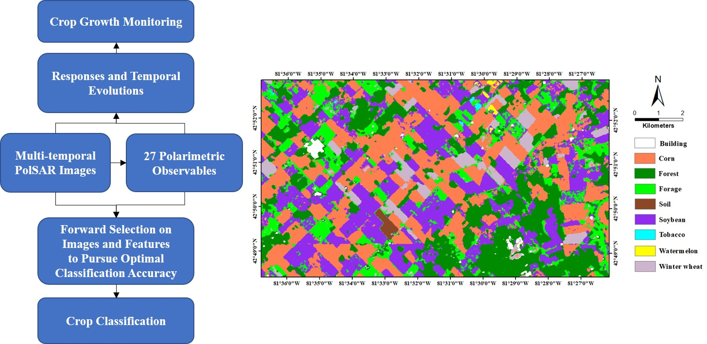
2. Materials and Methods

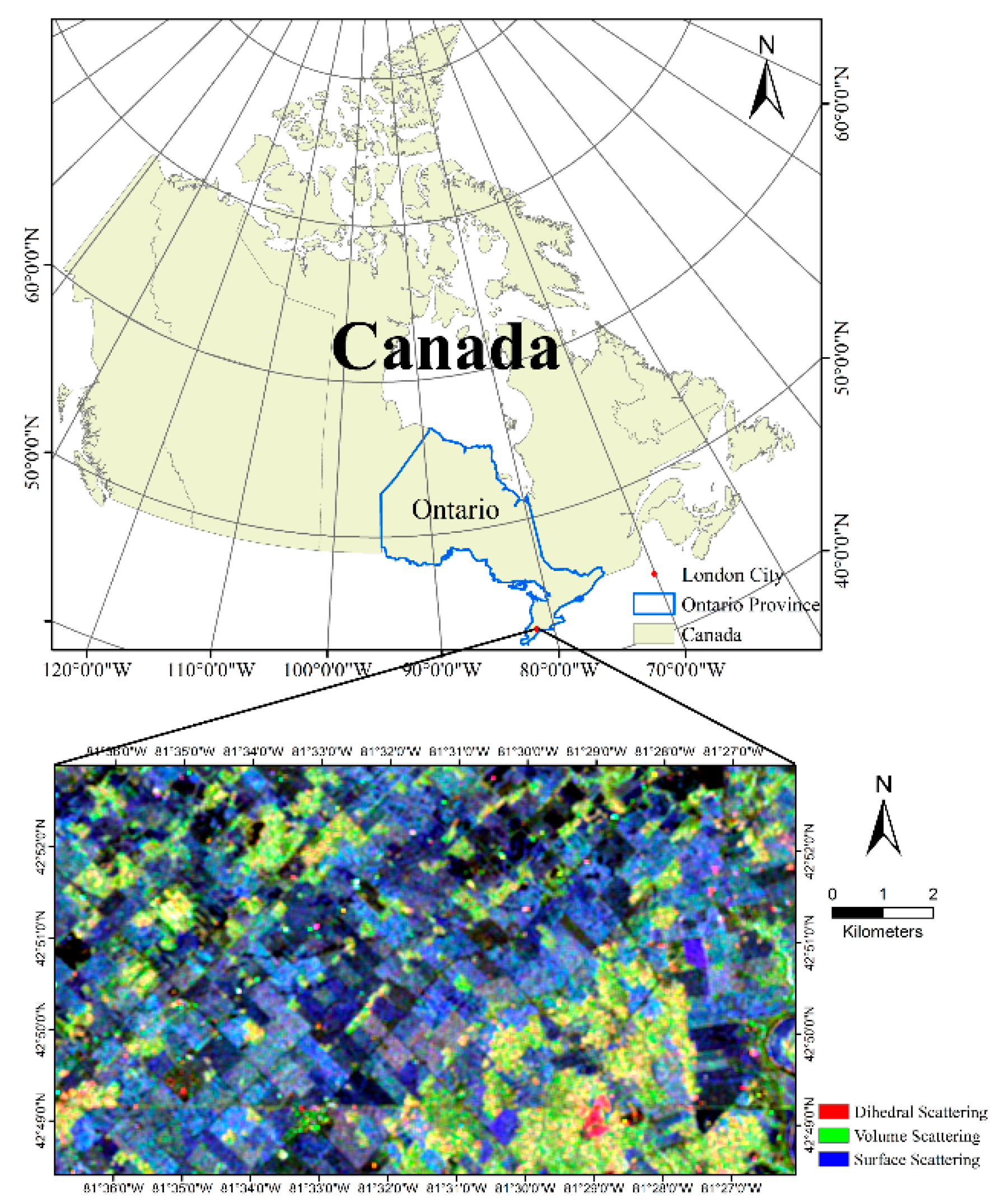
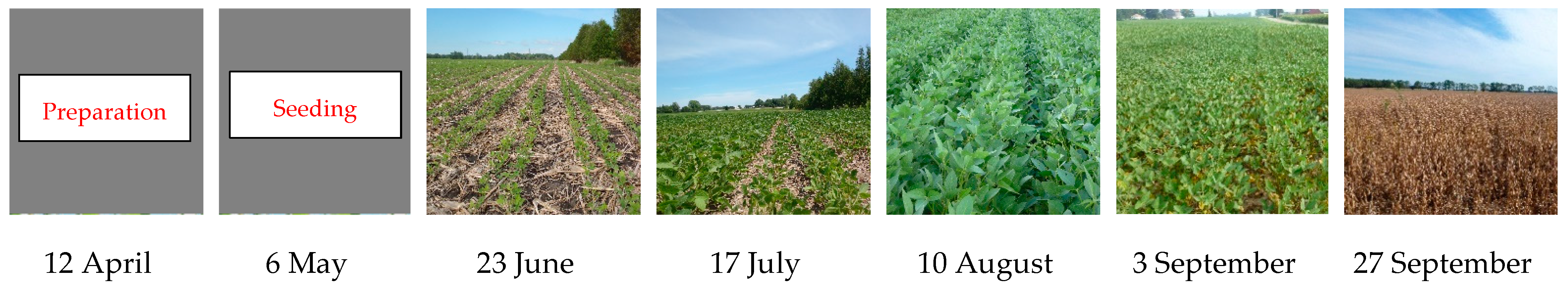
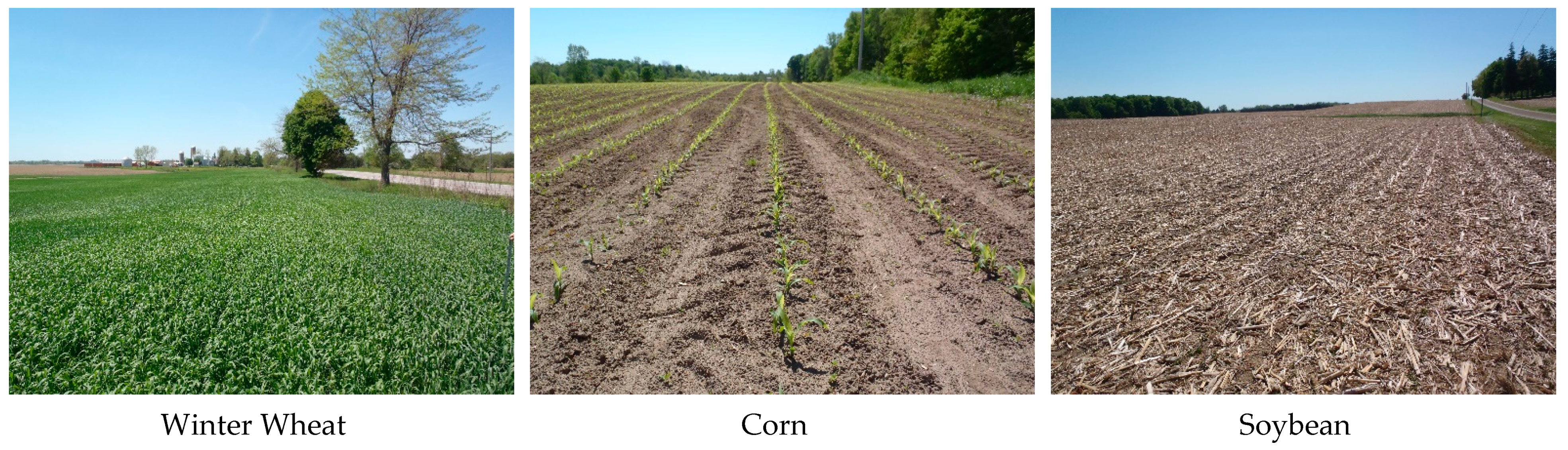
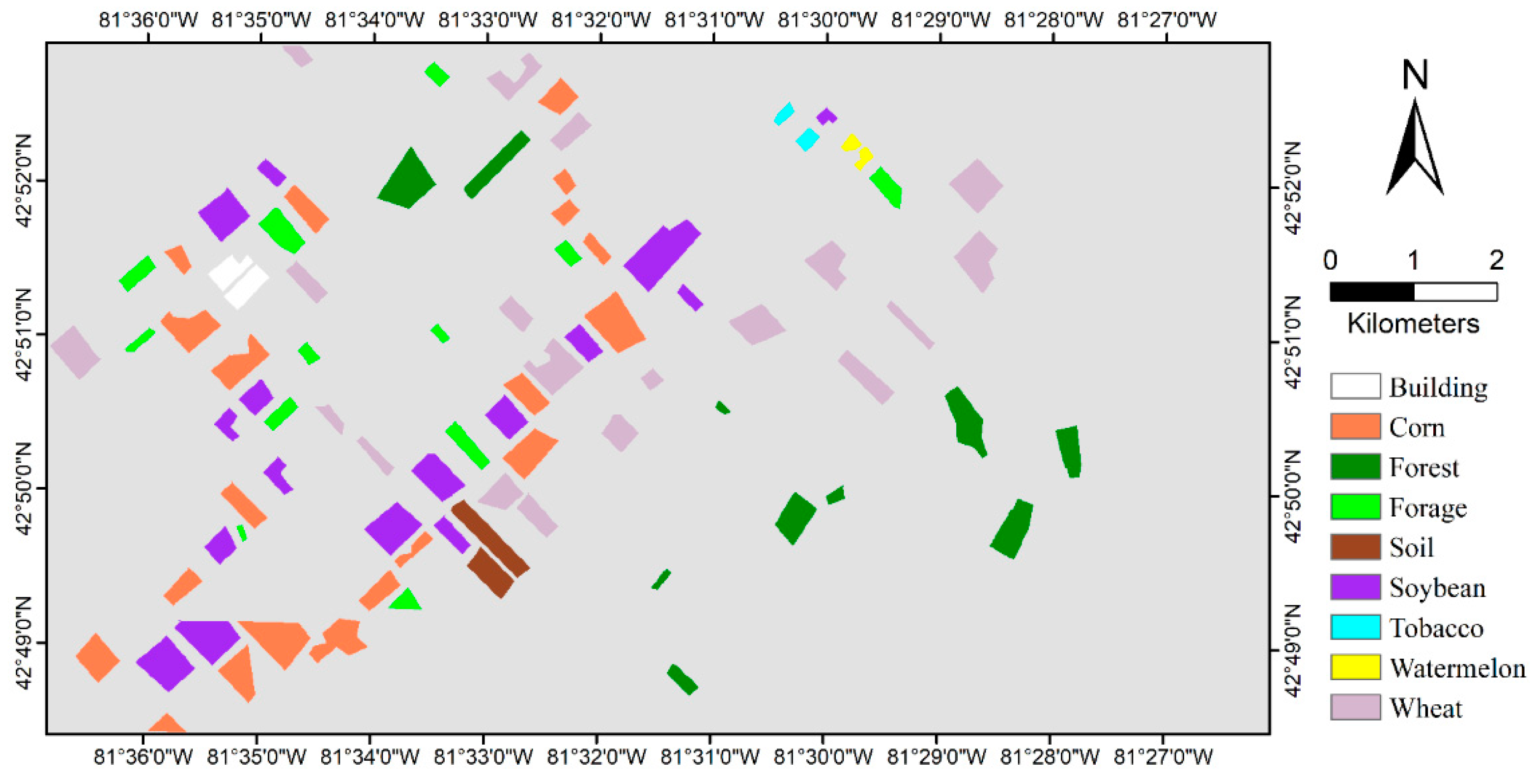
2.1. Study Site and Dataset

The study site is located in an agricultural area near the city of London in southwestern Ontario, Canada. The geographical location of this study area, and the Pauli RGB image corresponding to 12 April 2015 over the overlapping area of all RADARSAT-2 images, is presented in Figure 1. This site is very suitable for planting crops, attributed to abundant precipitation, mild weather and fertile soil, with relatively flat topography [39,41]. The main crop types over this site are winter wheat, corn, soybean and forage consisting of alfalfa, hay and grass. A few fields of tobacco and watermelon are also planted in this site. Almost all crops are rain-fed without irrigation. In addition to field crops, there are a few buildings and forest patches in the study area. The planting and harvest time for major crops in the study area are basically the same year by year. Corn and soybean are routinely seeded in May, ripened in September and harvested in October. In contrast, winter wheat is usually seeded in October of the previous fall, matured in July, and harvested from late July to early August the following year. Due to the long-time (November to March) of heavy snow in this region, farmers don’t start field operations until early April, and the winter wheat fields follow the same calendar to start regrowth around the same time. As crop rotations are commonly practiced in this region, crop residuals left from previous year’s harvest are mostly different from the crops seeded in the current year. For instance, the winter wheat fields are likely to have residues of corn or soybean prior to seeding at field preparation.

As shown in

Table 1. Description of available RADARSAT-2 time series overpassed the study area in 2015.

Date	Acquisition Mode	Incidence	Resolution	Orbit	Look Direction
12 April 2015	FQ10W	28.4~31.6°	5.5 m × 4.7 m	Ascending	Right
6 May 2015	FQ10W	28.4~31.6°	5.5 m × 4.7 m	Ascending	Right
23 June 2015	FQ10W	28.4~31.6°	5.5 m × 4.7 m	Ascending	Right
17 July 2015	FQ10W	28.4~31.6°	5.5 m × 4.7 m	Ascending	Right
10 August 2015	FQ10W	28.4~31.6°	5.5 m × 4.7 m	Ascending	Right
3 September 2015	FQ10W	28.4~31.6°	5.5 m × 4.7 m	Ascending	Right
27 September 2015	FQ10W	28.4~31.6°	5.5 m × 4.7 m	Ascending	Right

, seven fully polarimetric C-band RADARASAT-2 images in FQ10W (Fine-Quad Wide) covering the entire growing season from April to September in 2015 were employed. The uniform image acquisition beam mode offers the advantage of reduced complexity caused by varying SAR incidence angles for multitemporal studies [35,36,37]. In particular, except for the date on 30 May, when the satellite did not overpass our study area to acquire imagery due to user conflicts, the time interval between data acquisitions was 24 days.

From April to September 2015, field surveys were conducted every month by the Geographic Information Technology and Application (GITA) laboratory at the University of Western Ontario (UWO). Agricultural information, including crop type, crop height, soil moisture, crop phenological stage and field photos was recorded. Figure 2 shows field photos of three main crops (winter wheat, corn and soybean) on RADARSAT-2 acquisition dates. Since the corn and soybean were not emerging yet on 12 April and 6 May, there were no ground photos for corn and soybean taken on both dates. Field surveys of corn and soybean started on 23 May. Fields photos of three main crops on this date are presented in Figure 3. The heights of winter wheat were significantly taller than those of corn and soybean on 23 May. The winter wheat field was harvested from the end of July to early August and standing residuals were left; hence, field photos over winter wheat in harvested state were only taken once in August, as shown in Figure 1. From these field photos, we observed that the collected PolSAR time-series imagery covered the crops’ growth changes throughout almost the full growing season of the main crops over the study site. The dataset is very suitable for crop monitoring by analyzing the temporal evolution of the polarimetric parameters. The ground truth labels of crop types were collected in a field survey, and then we manually digitized the boundary of each field based on satellite imagery in a Geographic Information System (GIS). Each field polygon was drawn within the field boundaries to avoid mixed pixels. Finally, these polygons were converted to a raster layer with the same spatial resolution as the remote sensing data. During the field surveys, a total of 85 fields were identified. The land-cover map of ground truth is shown in Figure 4. Training and testing datasets for crop classification and accuracy assessment were randomly selected at the field level without overlap. Additional details are presented in

Table 2. The identified crop fields and the number of pixels for classification training and testing.

Land Cover	Training Samples		Testing Samples
	Number of Pixels	Number of Fields	Number of Pixels	Number of Fields
Corn	6258	4	20,246	16
Soybean	6505	4	15,995	12
Forage	3700	5	3615	7
Winter wheat	6018	3	17,723	16
Watermelon	310	1	309	1
Tobacco	416	1	301	1
Forest	5148	4	7292	6
Built-up	1267	1	1117	1
Soil	2331	1	1592	1

.

2.2. PolSAR Observables

Different from single and dual polarization SAR systems that can only obtain one or two linear channel images over the target site, a fully polarimetric SAR system can acquire four images by alternately transmitting two radar signals with an orthogonal polarization basis (e.g., H or V), and receiving backscattered signals simultaneously (H and V). The acquired data can be represented, for instance in an H-V polarization basis, by a $2\times 2$ complex Sinclair scattering matrix S as [28,29]

$$S=\left[\begin{array}{cc}{S}_{HH}& S_{HV}\\ S_{VH}& S_{VV}\end{array}\right]$$

(1)

where $S_{HH}$ and $S_{VV}$ represent the complex backscattering coefficients as the transmitted polarization and received polarization are the same (i.e., the copolarized channels), while $S_{HV}$ and $S_{VH}$ denote the complex backscattering coefficients in the cross-polarized channels. Under the assumption of reciprocal scattering, S_HV and $S_{VH}$ are considered equal [28,29].

Since the scattering matrix is commonly affected by speckle noise, and distributed targets are common in natural media, incoherent polarimetric analysis by using second-order statistics, such as the covariance matrix or the coherency matrix, are given more attention [28,29]. The corresponding covariance matrix C and the coherency matrix T are represented as [28,29]:

$$C=\left[\begin{array}{ccc}〈{\left|S_{HH}\right|}^2〉& \sqrt{2}〈S_{HH}{S}_{HV}^{\ast }〉& 〈S_{HH}{S}_{VV}^{\ast }〉\\ \sqrt{2}〈S_{HV}{S}_{HH}^{\ast }〉& 2〈{\left|S_{HV}\right|}^2〉& \sqrt{2}〈S_{HV}{S}_{VV}^{\ast }〉\\ 〈S_{VV}{S}_{HH}^{\ast }〉& \sqrt{2}〈S_{VV}{S}_{HV}^{\ast }〉& 〈{\left|S_{VV}\right|}^2〉\end{array}\right]$$

(2)

$$T=\frac{1}{2}\left[\begin{array}{ccc}\langle {\left|S_{HH}+S_{VV}\right|}^2\rangle & \langle \left(S_{HH}+S_{VV}\right){\left(S_{HH}-S_{VV}\right)}^{\ast }\rangle & 2\langle \left(S_{HH}+S_{VV}\right)S_{HV}^{\ast }\rangle \\ \langle \left(S_{HH}-S_{VV}\right){\left(S_{HH}+S_{VV}\right)}^{\ast }\rangle & \langle {\left|S_{HH}-S_{VV}\right|}^2\rangle & 2\langle \left(S_{HH}-S_{VV}\right)S_{HV}^{\ast }\rangle \\ 2\langle S_{HV}{\left(S_{HH}+S_{VV}\right)}^{\ast }\rangle & 2\langle S_{HV}{\left(S_{HH}-S_{VV}\right)}^{\ast }\rangle & 4\langle {\left|S_{HV}\right|}^2\rangle \end{array}\right]$$

(3)

In past studies, a large number of polarimetric observables were extracted from these polarimetric matrices (i.e., C or T in Equations (2) and (3)) for crop monitoring applications [24,42,43,44]. For instance, a global sensitivity analysis of 20 PolSAR observables for crop biophysical variable estimation were investigated in [43]. However, the number and types of selected PolSAR observables for investigating temporal evolutions and crop classification were usually limited. Besides those 20 polarimetric observables in sensitivity studies, according to wide usage of PolSAR observables in crop monitoring studies, a total of 27 polarimetric observables were selected for temporal evolution inspection and considered as input features for crop classification in this study, as listed in Table 2. For the convenience of subsequent analysis, the 27 polarimetric observables were categorized into 10 groups and given their abbreviations. First, groups 1–3 were the widely used backscattering power related parameters including SAR backscattering coefficients in linear polarization basis (HH, HV, VV), backscattering coefficients in the Pauli basis (HH + VV, HH-VV) and total backscattering power (Span). These parameters can be directly extracted or computed following simple operations from the elements in either the covariance matrix or coherency matrix. Three backscattering ratios (HH/VV, HV/HH, and HV/VV) sensitive to target characteristics were also considered, which can be obtained from the covariance matrix and classified as group 4. The polarimetric complex coherences between polarimetric channels were also selected, which have been often used for crop phenology monitoring and crop growth stage identification [24,25,31,36]. For two polarization channels i and j, the polarimetric complex coherence is given as [45]:

$${\rho }_{ij}=\frac{〈S_i{S}_j^{\ast }〉}{\sqrt{〈{\left|S_i\right|}^2〉/{\left|S_j\right|}^2〉}}$$

(4)

where <> denotes the sample average. Four complex correlation coefficients were employed, which can be split into four amplitudes and four phases marked as group 5 and group 6. In past studies, polarimetric target decomposition has proven to characterize scattering mechanisms and been frequently used for generating polarimetric features in agricultural applications. Two mostly representative methods, i.e., the Freeman-Durden three-component decomposition [46], and the H-A-alpha decomposition proposed by Cloude and Pottier [47], were used. In addition, a recent study has shown that a model-based decomposition method, i.e., Neumann decomposition [48], might be more effective in improving the crop classification accuracy with respect to the Cloude-Pottier decomposition [41]. Therefore, Neumann decomposition was also employed in our study. Three decomposition methods were marked as groups 7–9. In addition, the radar vegetation index (RVI) [49] is highly sensitivity to crop parameters [50,51,52]; thus, it was used in this study and marked as group 10. The expression of RVI is defined as [53]:

$$RVI=\frac{4min\left({\lambda }_1,{\lambda }_2,{\lambda }_3\right)}{{\lambda }_1+{\lambda }_2+{\lambda }_3}$$

(5)

where λ₁, λ₂, λ₃ are the eigenvalues of the covariance/coherency matrix.

2.3. Data Processing

A series of preprocessing steps including radiometric calibration, polarimetric matrix generation, speckle filtering and geocoding, were conducted for each RADARSAT-2 image used. A boxcar filter with a 9 by 9 window was employed to suppress the speckle noise. A 30 m digital elevation model product (PDEM) of Ontario, Canada, was applied to geocode the polarimetric matrix in the Universal Transverse Mercator (UTM) geographic reference with an output cell resolution of 10 m by 10 m. Afterwards, for each acquisition date, 27 feature images of polarimetric parameters, listed in

Table 3. The list of 27 polarimetric observables in 10 groups selected for temporal evolutions and classification in this study.

Group	Polarimetric Observable	Description	Abbreviation
1	HH (C11), HV (C22), VV (C33)	Backscattering coefficients in the linear polarization channels	LP
2	HH + VV (T11), HH-VV (T22)	Backscattering coefficients in the Pauli polarization channels	Pauli
3	Span	Total backscattering power	Span
4	HH/VV, HV/HH, HV/VV	Backscattering ratios	Ra
5	${\mathsf{\rho }}_{HHVV},{\mathsf{\rho }}_{HVVV},{\mathsf{\rho }}_{HHHV},{\mathsf{\rho }}_{HH+VV,HH-VV}$	Correlation between polarimetric channels	Ro
6	${\varphi }_{HHVV},{\varphi }_{HVVV},{\varphi }_{HHHV},{\varphi }_{HH+VV,HH-VV}$	Phase difference between polarimetric channels	Pha
7	$P_s,P_d,P_v$	Scattering power from different scattering mechanisms derived from Freeman-Durden decomposition	FD
8	$\mathrm{H},\mathrm{A},\mathsf{\alpha }$	Entropy, anisotropy, alpha angle from Cloude-Pottier decomposition	CP
9	$\left|\mathsf{\delta }\right|,{\mathsf{\varphi }}_{\delta },\mathsf{\tau }$	Magnitude and phase of the particle scattering anisotropy, the degree of orientation randomness derived from Neumann decomposition	ND
10	RVI	Radar Vegetation Index	RVI

, were extracted. These images had the same geometry and pixel spacing of 10 m.

2.4. Experimental Design

For crop growth monitoring, the temporal evolutions of all polarimetric observables for each crop type used as input feature layers for classification were derived. First, the locations of the fields for each crop type were extracted from the ground truth set. Afterwards, the average values of polarimetric observables from all the ground truth fields for each crop type were produced on each RADARSAT-2 acquisition date. The analysis of temporal evolutions of polarimetric observables were more focused on the three major crops (corn, soybean, and winter wheat).

For crop classification, 27 polarimetric observables for each SAR image were obtained and combined differently as the input feature layers according to ten groups defined in Table 3. As a result, 10 combinations of input layers were constructed. The detailed descriptions of the combinations of polarimetric observables are presented in

Table 4. The detailed descriptions of the combinations of input polarimetric observables. Note that abbreviations are explained in Table 2.

Data Source	Polarimetric Observables	Number of Images	Number of Layers
LP	HH (C11), HV (C22), VV (C33)	7	21
Pauli	HH + VV (T11), HH-VV (T22)	7	14
Span	Span	7	7
Ra	HH/VV, HV/HH, HV/VV	7	21
Ro	${\mathsf{\rho }}_{HHVV},{\mathsf{\rho }}_{HVVV},{\mathsf{\rho }}_{HHHV},{\mathsf{\rho }}_{HH+VV,HH-VV}$	7	28
Pha	${\varphi }_{HHVV},{\varphi }_{HVVV},{\varphi }_{HHHV},{\varphi }_{HH+VV,HH-VV}$	7	28
FD	$P_s,P_d,P_v$	7	21
CP	$\mathrm{H},\mathrm{A},\mathsf{\alpha }$	7	21
ND	$\left|\mathsf{\delta }\right|,{\mathsf{\varphi }}_{\delta },\mathsf{\tau }$	7	21
RVI	RVI	7	7

. The frequently used Random Forest (RF) algorithm was applied to each combination in this study due to its good performance, and demonstrated advantages in crop classification [39,54,55,56]. In addition, a beneficial property of RF is that it can quantify variable importance for classification [57,58]. Previous studies have shown that accuracy of crop classification with RF nearly reaches stable values as the number of decision trees increases above 50 [39,41,56]. Finally, 100 decision trees were used in RF algorithm for all classification tests in this study.

In total, ten groups of polarimetric observables were used as input features in classification. The combination of all types of polarimetric observables is usually adopted for crop classification and commonly generates better results than using single types of polarimetric observables alone. However, contributions from different features to crop classification accuracy may vary dramatically. Therefore, it is interesting to determine an optimal combination of features that could obtain the best classification accuracy. Moreover, in past studies with multitemporal SAR data, comparable, or even better crop classification accuracies, were sometimes obtained by combining a few images acquired at certain critical phenology stages [7,10,24,26]. Moreover, using fewer images can reduce the cost and computational burden of image processing and classification. Therefore, it is also worth studying the optimal combination of SAR images that could gain an acceptable classification accuracy. In addition, further investigating optimal combination of both factors, i.e., polarimetric observables and SAR images. will be an interesting topic.

Recently, a forward selection procedure was proposed for searching the optimal combination of SAR images that make the best tradeoff between classification and number of images [7]. In this procedure, the SAR images for classification were gradually selected and included in the image set (starting with an empty image set) with an increment step of one acquisition date. The concept of the forward selection procedure can be expanded in search of the optimal combination of polarimetric observables for crop classification, i.e., forward feature selection. In detail, the groups of polarimetric observables for classification were gradually selected and included in the feature set (starting with an empty feature set) with an increment of one group, and the feature combination with the best classification accuracy was chosen at each step.

Therefore, we first conducted RF classifications with single groups of polarimetric observables and compared their performances. Then, the classification experiments were focused on investigating optimal combinations. A forward selection procedure was applied for searching the optimal combination of polarimetric observables, SAR images or both aspects. The experiments were designed to make the best tradeoff between classification accuracy and number of parameters, image acquisitions or both factors. First, all SAR images were selected in RF classifications by the forward feature selection procedure. For instance, RF classifications with single groups of polarimetric observables were tested in the first step. The optimal combination of polarimetric observables was obtained. Then, all polarimetric observables were selected in RF classifications by the forward image selection procedure. For instance, RF classifications using single images (one acquisition date) were tested in the first step. Finally, RF classifications were carried out again using the optimal combination of polarimetric observables by the forward image selection procedure.

Classification performance was affected by the training and testing samples, including both the number of samples and their distribution. To investigate the impact of the training and testing samples on the overall classification performance, the classification tests for the optimal combination SAR image produced by a forward image selection procedure using all polarimetric observables were carried out again by swapping the training and testing samples in Table 2. Moreover, based on the unique capability of the RF method, the variable importance contributing to crop classification was also quantified. The RF classification with all polarimetric observables using all RADARSAT-2 images was selected to investigate the relative importance of the input variables for crop classification.

3. Results

3.1. Temporal Evolution of Polarimetric Observables

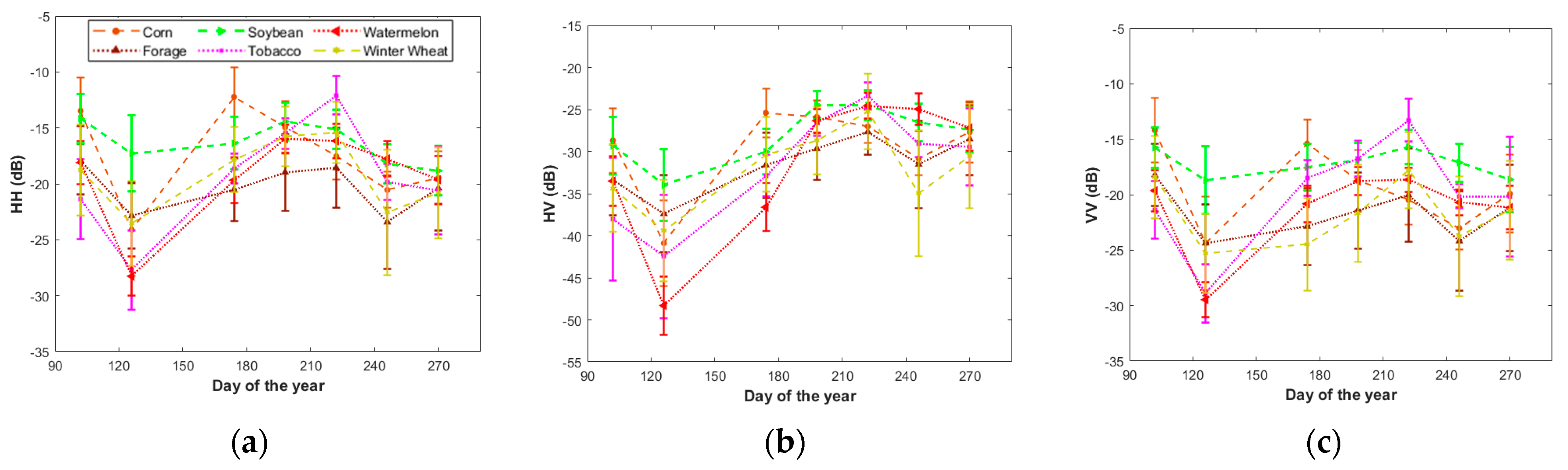
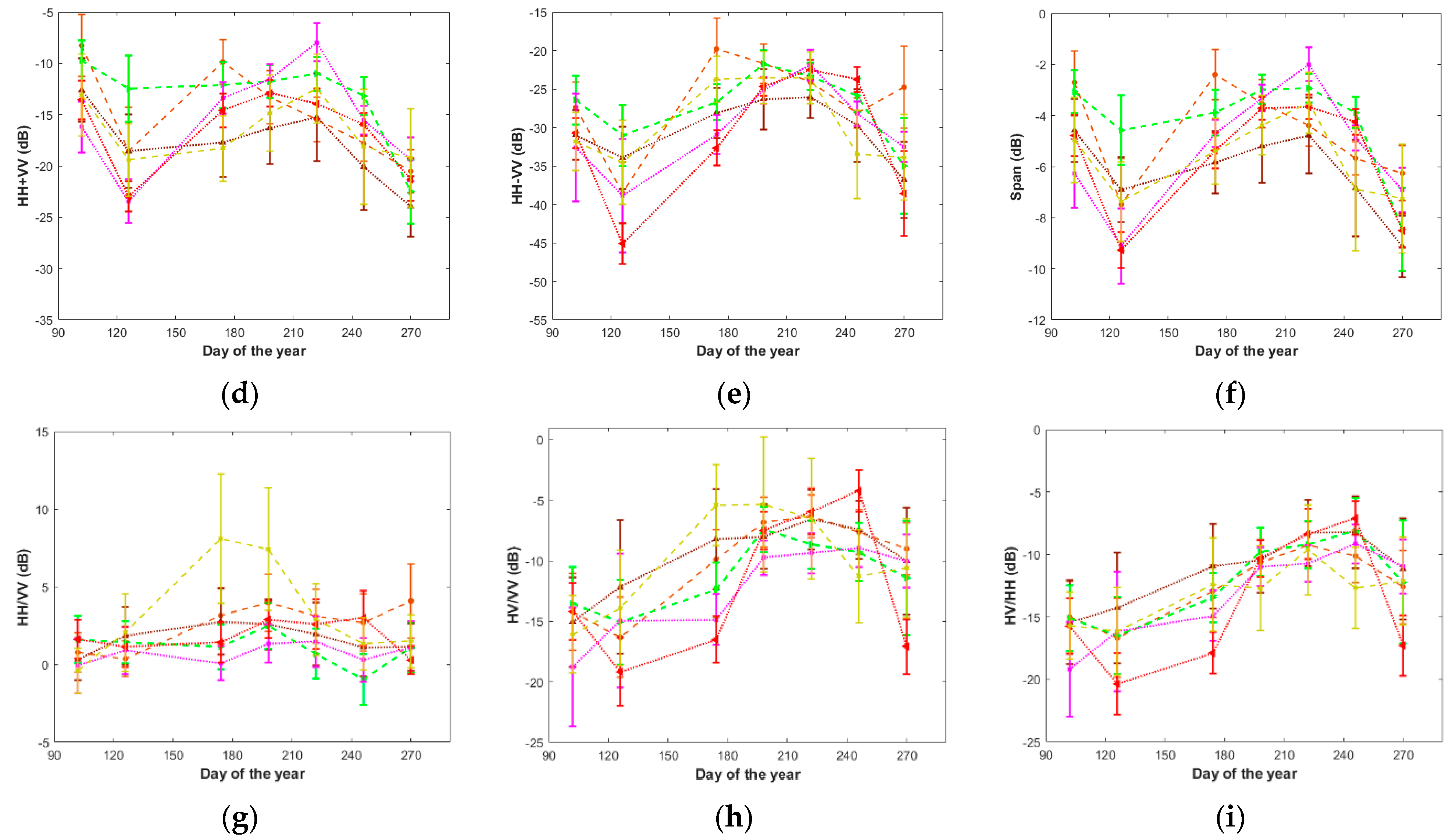
3.1.1. SAR Backscattering

The average SAR backscattering coefficients in linear polarization (HH, HV, VV), Pauli channels (HH + VV, HH-VV), total scattering power (Span), and backscattering ratios (HH/VV, HV/VV, HV/HH) for various crops throughout the whole growing season were calculated and are presented in Figure 5 (The values of three main crops (corn, soybean, and winter wheat) are shown in the supplementary Table S1). In general, the seasonal patterns of HV and HH-VV were more pronounced than those of co-polarizations (HH, VV), Span, and HH + VV. Taking winter wheat as an example, the dynamic range of HV was about 14 dB, and that of HH-VV was approximately 10 dB, while it was about 6 dB in HH and VV, 7 dB in HH + VV, and only about 3 dB in Span. The seasonal pattern of crops under HV was the most obvious, so the subsequent analysis of the variation of radar scattering values mainly revolved around HV polarization.

The seasonal patterns of winter wheat and summer crops are clearly shown in HV. In the study area, winter wheat is sown in October of the previous year, going through dormancy over winter, and starts regrowth when the snow melts the following spring. During the month of April and early May, the HV value was relatively low due to the small biomass of the winter wheat crop. After the weather warmed up more, it started to grow from May to August, and the HV value continued to rise (−40 dB to −25 Db). In mid-August, after winter wheat had been harvested, the HV value showed a downward trend. Watermelon and tobacco are harvested in October after a rapid increase in HV values during sowing and emergence in May, reaching peak biomass in August, and entering senescence in early August, when HV values start to decrease. The difference between watermelon and tobacco is that the HV values fluctuated very little from mid-July to October (−25 dB to −27 dB) for watermelon. The HV response value of soybean was the lowest in the sowing period (early May), and the HV value increased slowly and continuously to mid-July with crop growth. The HV value maintained a high value (about −24 dB) at the peak of biomass (mid-July and mid-August), and then decreased slowly due to aging and harvesting. The difference between corn and all other crops is that its biomass peaks in late June when the HV value reached its peak (about −25 dB), maintained a large HV value (about −26 dB) from late June to mid-July, and then began to decline.

The average values of three backscattering ratios (HH/VV, HV/VV, and HV/HH) for various crops were calculated and are shown in Figure 5g–i. It can be seen from the figures that most crops were more sensitive to HV/VV and HV/HH than to HH/VV, which showed only a clear temporal pattern for winter wheat. Most crops, such as corn, forage, soybean, tobacco, and watermelon, had stable HH/VV values (about 0–5 dB) throughout the growing season. The variation range of HH/VV value of soybean was 2 dB, and the variation range of HV/VV and HV/HH of soybean was about 8 dB and 9 dB. The variation range of HH/VV and HV/VV values of winter wheat was 9 dB, while the variation range of HV/HH was 5 dB, indicating that winter wheat was more sensitive to HH/VV and HV/VV. In conclusion, all crops except winter wheat were more sensitive to HV/VV and HV/HH. From Figure 5h,i, in general, the HV/VV value of crops was more pronounced than the HV/HH ratio. For example, the variation range of HV/VV of corn, tobacco and watermelon was 10 dB, 9 dB, and 16 dB respectively, and the variation range of HV/HH was 7 dB, 8 dB and 14 dB. Therefore, the following analysis mainly focuses on the HV/VV ratio.

Soybean and corn exhibited very similar patterns in HV/VV. The range of variation was small; the value from mid-July to late September was larger and more stable, which can be distinguished from other crops. When winter wheat biomass peaked in late June, the response of HV increased, so the HV/VV also reached the peak. Other crops peaked mainly from July to September, such as corn, which peaked in mid-August. The peaks for forage, tobacco and watermelon all occurred in early September. Tobacco showed a steady state of HV/VV (about −10 dB) from mid-July to late September. The variation of watermelon was the clearest, with a continuous upward trend from May to September, reaching a very high peak (−4 dB), and then decreased from September to October.

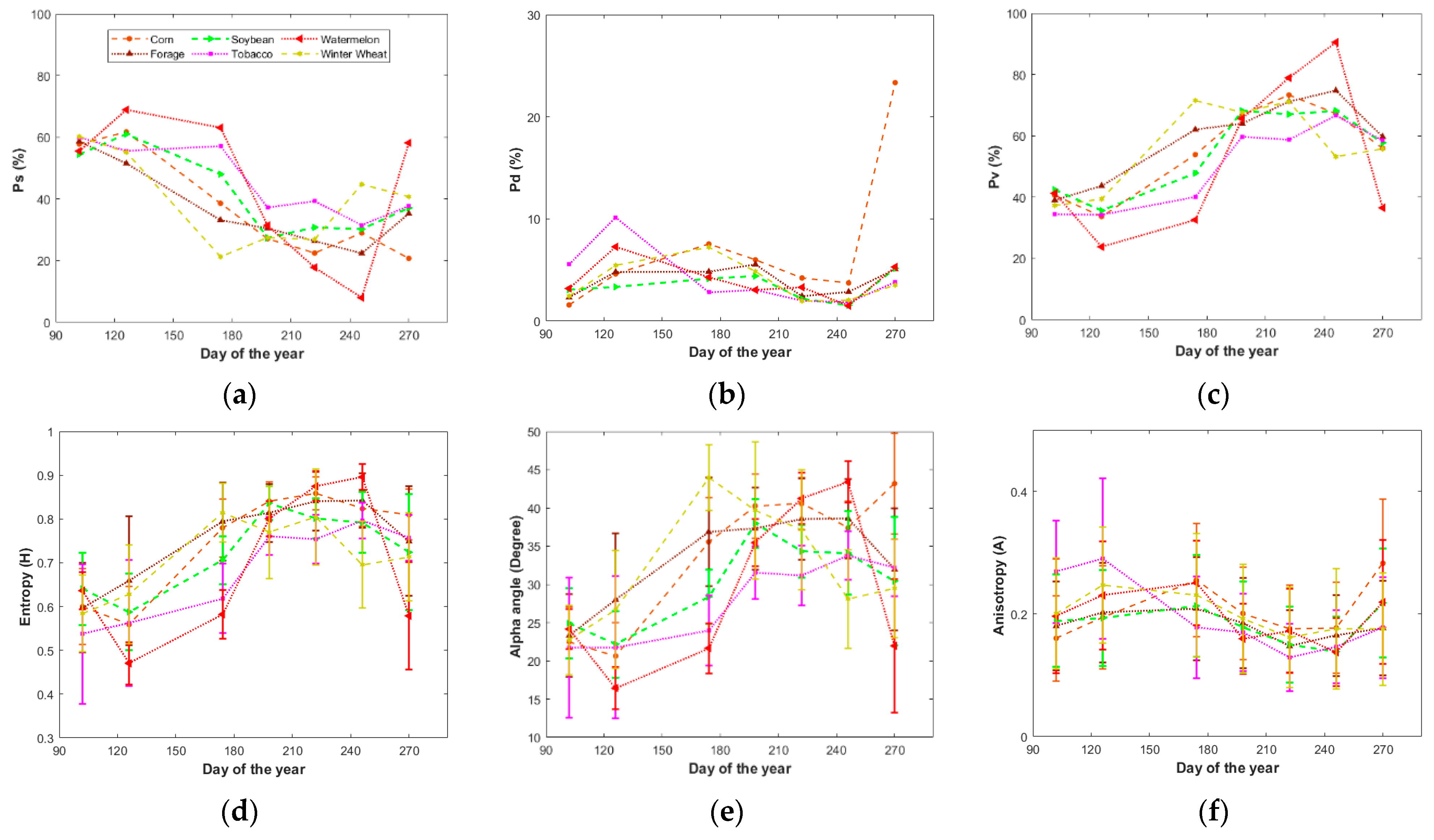
3.1.2. Polarimetric Decompositions

• Freeman-Durden Decomposition

The relative strength of the different scattering mechanisms present in the scene can be explained directly in terms of the proportional scattering contribution, in percentage (%), reported by Freeman-Durden decomposition. Notably, their proportional contribution varied greatly during the growing season for all crops. Figure 6a–c shows the contribution of surface scattering, double-bounce scattering and volume scattering of various crops during the growing season (The values of three main crops (corn, soybean, and winter wheat) in Figure 6 are shown in the supplementary Table S2). In general, the double-bounce contribution was small (less than 10%) for all crops, but for corn at the last date was 20%. The evolution of the scattering mechanism contributions was similar for all crops, showing a decreasing trend of surface scattering and an increasing trend of volume scattering. For tobacco, surface scattering was the main scattering mechanism from April to the end of June, while volume scattering was the main scattering mechanism from July to the end of September. The watermelon field and forage also had similar situations, for example, the contribution of surface scattering in the watermelon field accounted for 43%, and volume scattering accounted for 52% in the whole growing season. From August to September, the surface scattering of corn increased while volume scattering decreased, and the opposite trend was found in the watermelon field. For summer crops, volume scattering was dominant in soybean (>55%) throughout the growing season, although there was also a high contribution of surface scattering (>50%) from April to May. For corn, the volume scattering was dominant in the whole growing season (about 56%), from April to May but surface scattering was dominant (greater than 55%), in June to the end of September because of the crop leaf blight and part of the crop began to be harvested, so the volume was the main scattering mechanism (greater than 60%). Due to leaving crop residue after harvesting, double-bounce scattering also increased in the last date. Surface scattering was dominant in winter wheat from April to June (>50%), and volume scattering was dominant from June to August (>60%) due to canopy or standing residues.

• Cloude-Pottier Decomposition

Cloude-Pottier decomposition can determine the main scattering mechanism of targets on the land surface from the H-α characteristic plane. The variation trend of entropy (H), anisotropy (A), and α angle of various crops are reflected in Figure 6d–f. In general, most crops showed multiple scattering mechanisms with moderate to high values of entropy. The maximum entropy for most of crops appeared in August and September, while winter wheat reached maximum entropy at its peak biomass in late June, and soybean achieves the maximum entropy in July. Entropy generally showed a similar change trend in the whole growing season. It first increased and then tended to be relatively stable at the late stages. During the whole observation period, the α angle identifying the average scattering mechanism was distributed in the range between 14° and 45° for the three crops, indicating an increasing contribution of volume scattering, which is consistent with the contribution of scattering mechanism obtained by Freeman-Durden decomposition. Anisotropy of all crops was around 0.2 along the season, indicating that in addition to the main scattering mechanism at each stage, the difference between the second and third scattering mechanisms was relatively small.

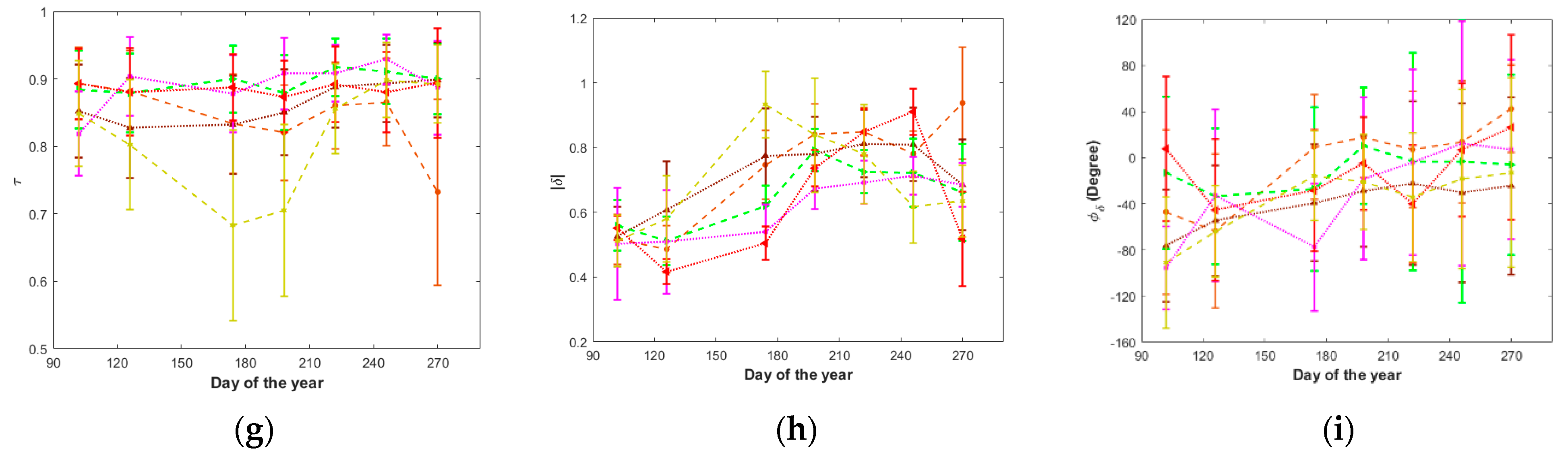
• Neumann Decomposition

The Neumann decomposition outputs three parameters, namely the degree of orientation randomness (τ), the magnitude of particle scattering anisotropy $\left|\delta \right|$ and the phase of the particle scattering anisotropy${\varphi }_{\delta }$ [48]. In addition, the parameter$\left|\delta \right|$ can represent the scattering mechanism type if a mixed scattering mechanism is assumed [48]. Figure 6g–i shows the temporal variation of the three parameters. According to Figure 6g, the τ value of most crops was large (>0.8) and maintained a stable state throughout the growing season, indicating that the scattering randomness of crops during the whole growing season was large. The variation of winter wheat was the most obvious. From Figure 6h, it is clear to the seasonal patterns of $\left|\delta \right|$in all crops showed large variations and were very similar to the α angle from the Cloude-Pottier decomposition, which proves its usability in scattering mechanism interpretation. In Figure 6i, the variations of ${\varphi }_{\delta }$ among different crops are quite different, providing helpful information for further distinguishing crop types.

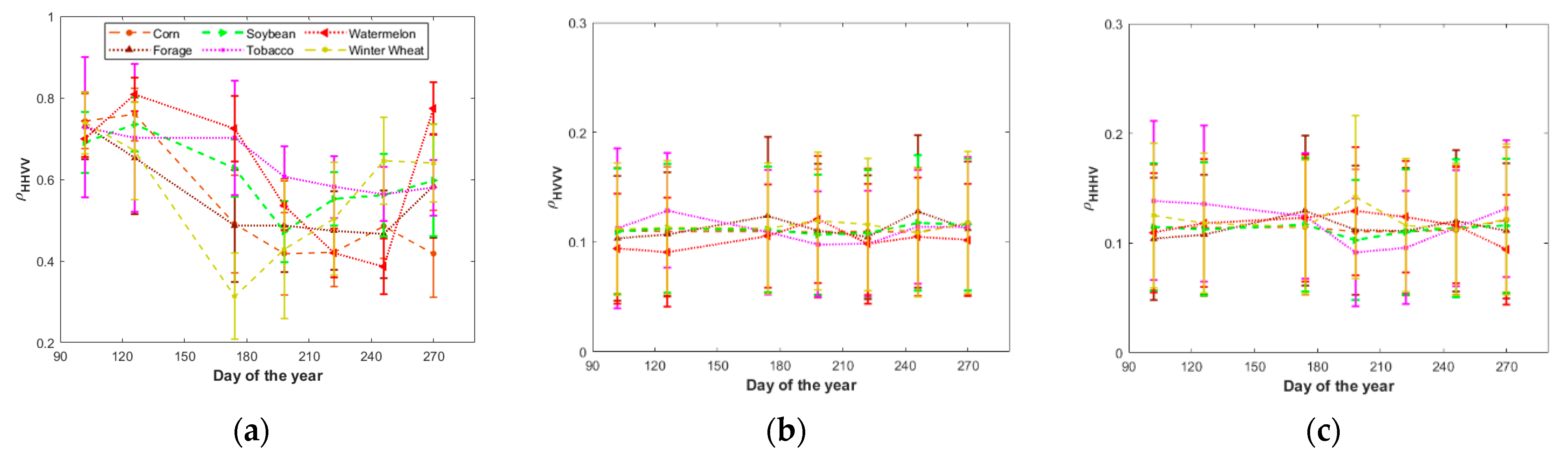
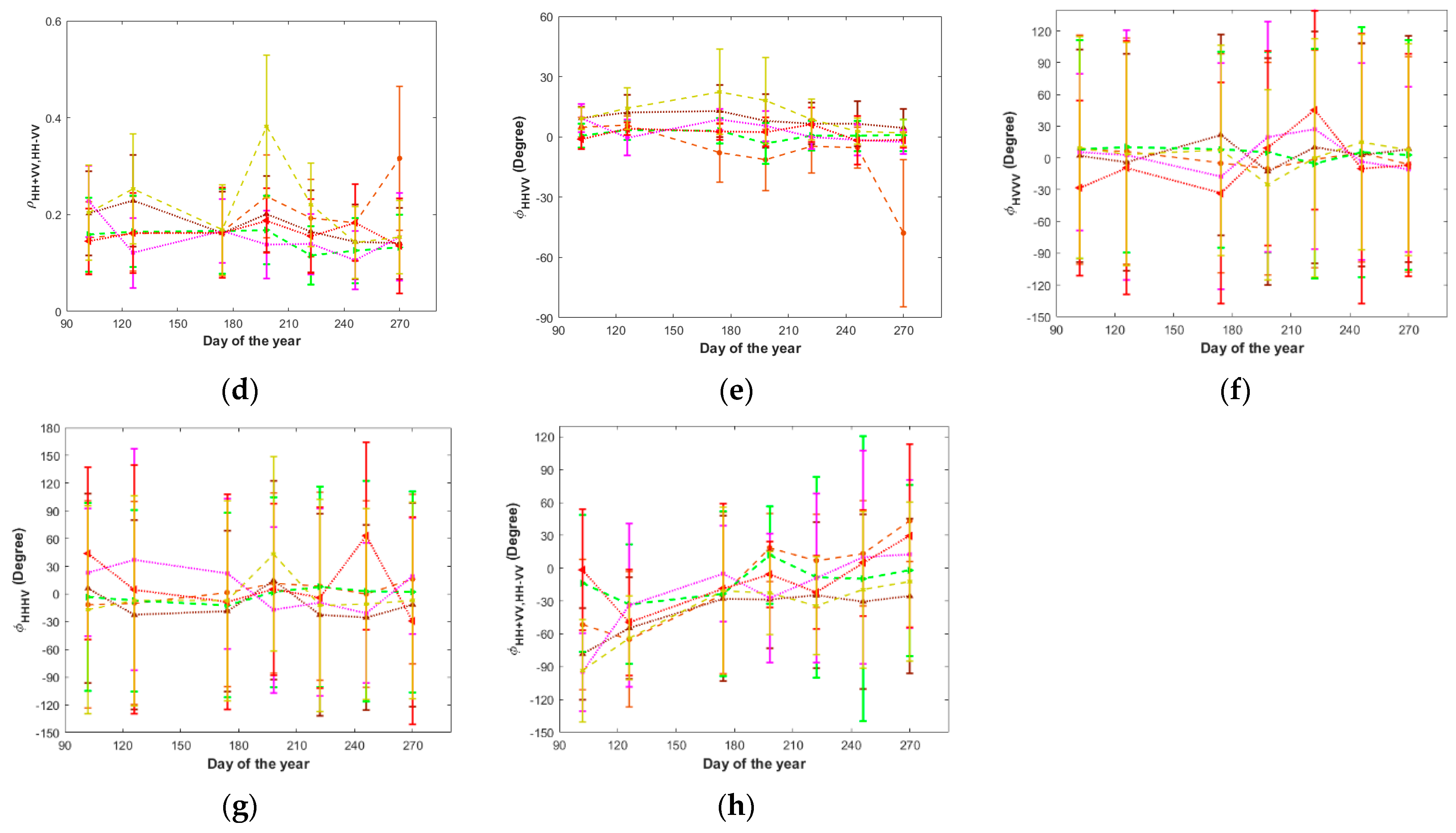
3.1.3. Correlation Coefficient and Phase Difference

Polarimetric complex coherences contain two parameters, the correlation coefficient and the phase difference between two polarimetric channels, which can be used to help distinguish land cover types. Figure 7 shows the temporal variations of the common four complex correlation coefficients (The values of three main crops (corn, soybean, and winter wheat) are shown in the supplementary Table S3). It can be seen that ${\mathsf{\rho }}_{\mathrm{HHVV}}$ showed more sensitivity to crop development than ${\mathsf{\rho }}_{\mathrm{HVVV}}$, ${\mathsf{\rho }}_{\mathrm{HHHV}}$, and ${\mathsf{\rho }}_{\mathrm{HH}+\mathrm{VV},\mathrm{HH}-\mathrm{VV}}$, whereas all phases were rather noisy due to the low correlations found in most part of the growing season.

In Figure 7a, the copolarization correlation coefficient ${\mathsf{\rho }}_{\mathrm{HHVV}}$ of corn, soybean, watermelon and winter wheat show a gradually decreasing trend first followed by an increasing trend in the growing season. The volume scattering increased with the progression of crop growth, and the surface scattering decreased with the increase of crop coverage and biomass accumulation throughout the vegetative growth period. When the crops started to mature, corn leaves started to dry up and bend down causing reduced volume scattering, and increased background soil became visible to the SAR signal, leading to increase in surface scattering. In the case of soybeans, in May to mid-July surface scattering was reduced and volume scattering increased (${\mathsf{\rho }}_{\mathrm{HHVV}}$ reduced from 0.7 to 0.5), while in late July to September volume scattering increased. Opposite trends were observed in watermelon, forage and tobacco when the surface scattering of other crops (corn and winter wheat) increased, and volume scattering decreased from August to September. The copolarization correlation of corn in April and May was high (about 0.7), by the middle of May and July it was on the decline (0.7 to 0.4), and then a small amplitude appeared, increasing (about 0.4 to 0.5) until September, followed by a small decline (0.4), showing that in the early stage of corn planting surface scattering was larger and volume scattering increased, because after harvest the surface scattering increased. The surface scattering of winter wheat was greater from April to late June, and the volume scattering increased from July to late September.

3.1.4. RVI

The radar vegetation index (RVI) showed the evolution of the vegetation cover in the study area during the whole growing season, as shown in Figure 8 (The values of three main crops (corn, soybean, and winter wheat) are shown in the supplementary Table S4). The RVI value of most crops first showed a trend of gradual rise and then began to decline in August, indicating that with the growth of crops, the randomness of crops increases, and the structure of vegetation becomes more and more complex. The RVI of all crops reached a peak in August and September. Among the main crops (corn, soybean, and winter wheat), the RVI of soybean increased sharply with crop growth (from May to July), reaching the peak of RVI in July, and maintaining a relatively stable RVI value (about 0.6) from mid-July to September when leaves were flourishing, then RVI decreased due to the falling-off of leaves at senescence and harvest. The RVI of corn peaked in August and then decreased with senescence and harvest. Due to the unique sowing time, the RVI value of winter wheat was relatively high in late June. The variation trend of tobacco and forage was similar, but the fluctuation of RVI of tobacco was slightly larger than that of forage. The change of RVI in watermelon was the most obvious among all crops, especially during the mature period (September to October), when leaves withered and RVI showed a sharp decline.

3.2. Crop Classification

3.2.1. Classification with Single Groups of Polarimetric Observables

For accuracy assessment of RF classifications using different combinations of polarimetric observables (i.e., groups in Table 3), the detailed statistics of overall accuracy (OA), Kappa coefficient, as well as class-wise producer’s accuracy (PA) and user’s accuracy (UA), are listed in

Table 5. Accuracy assessment of RF classifications using different combinations of polarimetric observables. Note that abbreviations are explained in Table 3.

Crop Class	LP		Pauli		Span		Ra		Ro
	PA	UA	PA	UA	PA	UA	PA	UA	PA	UA
Corn	94.77	84.00	93.45	84.95	82.17	92.4	91.22	80.68	91.99	85.52
Forest	98.33	94.28	95.79	97.39	90.30	94.36	98.86	94.21	98.94	97.72
Grass	90.98	67.70	87.41	69.30	66.17	87.39	52.62	42.35	45.39	52.15
Soil	89.51	100.00	89.89	100.00	94.80	76.76	86.43	100.00	90.7	90.87
Soybean	92.64	92.36	95.54	90.13	82.14	90.7	81.72	90.89	86.23	89.26
Tobacco	62.13	99.47	65.12	97.03	50.26	63.12	25.17	63.56	28.24	95.51
Watermelon	68.28	100.00	80.91	98.04	53.22	58.9	21.17	100.00	43.37	89.93
Wheat	76.44	97.40	77.71	96.80	95.17	65.76	88.8	97.66	93.22	94.49
OA	89.19		89.45		84.23		86.34		88.66
Kappa	0.86		0.86		0.80		0.82		0.85
Crop Class	Pha		FD		CP		ND		RVI
	PA	UA	PA	UA	PA	UA	PA	UA	PA	UA
Corn	90.02	86.60	95.83	87.58	90.52	82.02	93.95	89.73	66.37	57.06
Forest	80.66	76.62	99.07	97.65	99.74	97.77	99.71	97.94	99.3	94.80
Grass	48.47	26.42	88.38	56.62	52.62	48.48	77.12	64.93	39.52	33.94
Soil	70.41	76.89	91.08	100.00	82.54	99.77	83.79	99.18	78.89	100.00
Soybean	79.33	76.35	94.43	93.31	83.2	87.47	88.92	91.25	61.47	63.94
Tobacco	2.33	10.45	55.81	91.30	28.57	100.00	32.23	100.00	16.85	45.19
Watermelon	1.29	40.00	71.84	98.67	52.1	81.73	55.66	96.09	30.74	62.09
Wheat	66.21	86.21	75.38	96.57	90.49	96.88	93.18	97.42	60.69	72.77
OA	76.69		89.64		87.67		91.57		65.64
Kappa	0.70		0.87		0.83		0.89		0.55

. The classification based on Neumann decomposition had the best OA and Kappa coefficient (91.57% and 0.89), while results from RVI time series showed the lowest OA and kappa coefficient (66.54% and 0.55). Regarding SAR backscattering parameters, both Pauli and LP parameters showed more accurate results than Span and Ra. As for the polarimetric decomposition parameters, the model-based decomposition methods (FD and ND) achieved better results than the eigenvalue-based decomposition method (CP). From the set of polarimetric complex coherence parameters, the RF classification with the correlation coefficients (Ro) temporal profile produced comparable results, with an OA of 88.66% and Kappa coefficient of 0.85, which were significantly better than those using the phase difference (Pha) time-series (OA = 76.69, Kappa coefficient = 0.70). From class-wise accuracies among RF classifications, it is evident that the user’s accuracies and producer’s accuracies showed variations among crops and selected polarimetric observables. The three main economic crops (corn, soybean and wheat) in the study area were taken as examples for further analysis. Except for using RVI, the classifications using other feature groups produced good results for corn mapping, with PA greater than 90% and OA greater than 0.8. For soybean identification, LP, Pauli and FD produced better results than others, with PAs and OAs larger than 0.9. For wheat mapping, CP, ND and Ro achieved more accurate results, with PAs and OAs larger than 0.9.

Figure 9 shows the classification maps obtained by the RF algorithm using the ten different combinations of polarimetric observables defined in Table 4. The overall clustering patterns in most of results were good, since the crop fields were discriminated well. However, there existed some scattered errors, especially in RVI results.

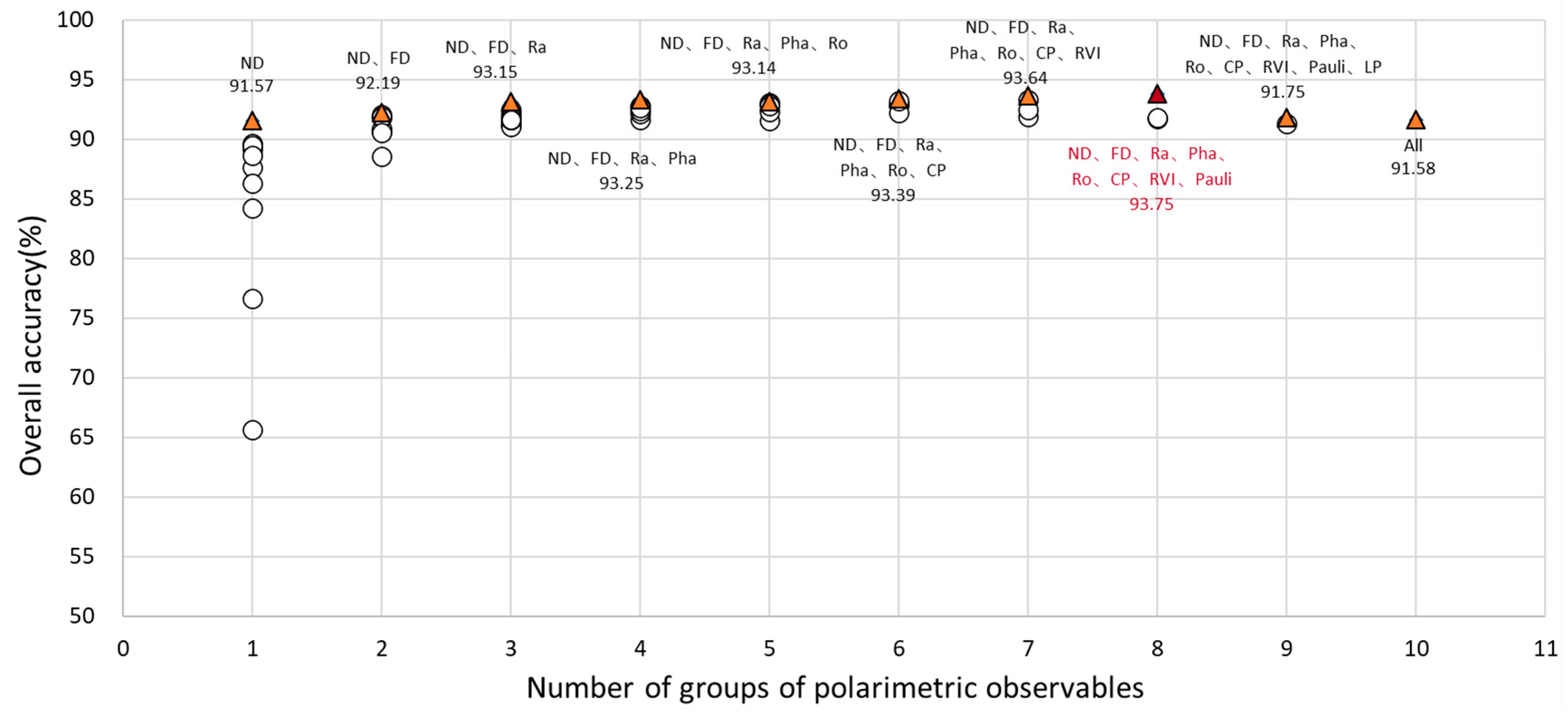
3.2.2. Optimal Combination of Polarimetric Observables

Figure 10 shows the RF overall accuracies for the optimal combination of polarimetric observables produced by a forward feature selection procedure using all multitemporal RADARSAT-2 images. A specific combination of eight groups (ND, FD, Ra, Pha, Ro, CP, RVI and Pauli) of polarimetric observables achieved the optimal crop classification accuracies in this study, with an OA of 93.75%. The corresponding optimal classification map is shown in Figure 11, which has better clustering patterns and less scattered errors than the maps in Figure 10. In addition, the usual combination of all features improved classification results in comparison with that using a single type of features alone. However, there were some combinations that produced better accuracies when using only two groups. This suggests that a reduced set of well-selected polarimetric features may generate better classification accuracies than using all features.

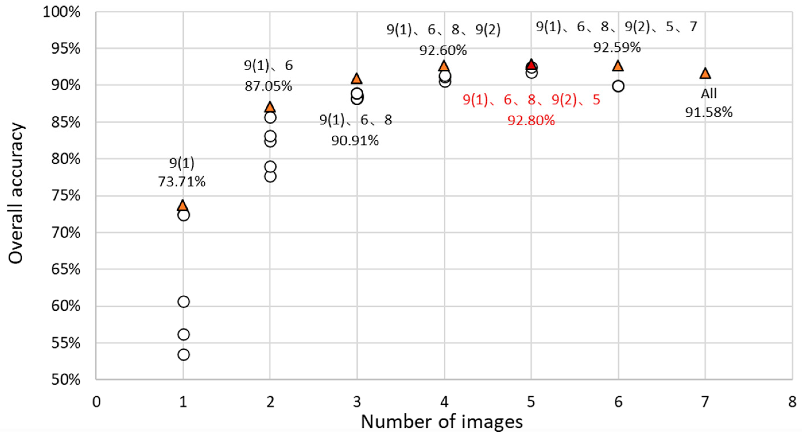
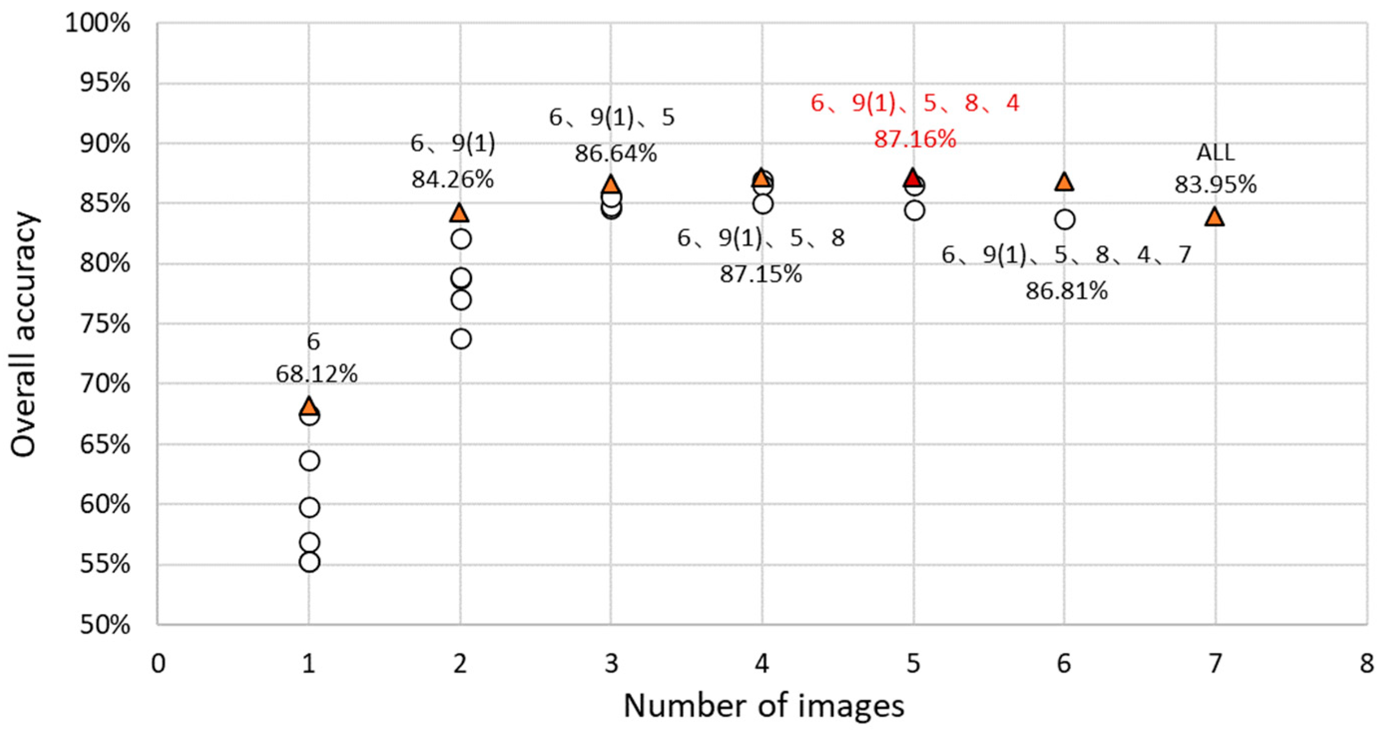
3.2.3. Optimal Combination of SAR Images

The corresponding accuracy assessment using single images (i.e., first step) with all polarimetric observables are listed in

Table 6. Accuracy assessment of RF classifications using single-date SAR image with all polarimetric observables.

Acquisition Date	OA (%)	Kappa
12 April 2015	46.11	0.32
6 May 2015	53.48	0.42
23 June 2015	72.56	0.65
17 July 2015	60.72	0.50
10 August 2015	56.23	0.45
3 September 2015	73.71	0.66
27 September 2015	72.44	0.65

. SAR images acquired in June and September produced more accurate results than at other dates. The reasons may be attributed to the large morphological and structural differences among crops on these dates due to the crop calendar. As can be seen from ground truth photos in Figure 4, big differences existed in June and September. In June, winter wheat was tall and dense while corn and soybean were sparse with large proportions of bare soil shown. In September, winter wheat had already been harvested, while corn and soybean were fully mature and started to senesce. In addition, there was a decrease in OA in the month of July and August. The reason might be corn and soybean have dense canopy structures and large canopy moisture, which increases difficulties for radar to distinguish them. Since the value of OA on September 3 was the largest in the first step, optimal combination in the next steps always included the image on this date. Figure 12 shows the RF overall accuracies for the optimal combination produced by the forward image selection procedure using all polarimetric observables. It is evident that some combinations produced better results than using all images, and the best OA was achieved using five images (in May, June, August, and September), with an OA of 92.80%. In addition, it indicates that the summer and autumn acquisitions (from June to September) were more valuable for crop classification than the spring acquisitions (April and May).

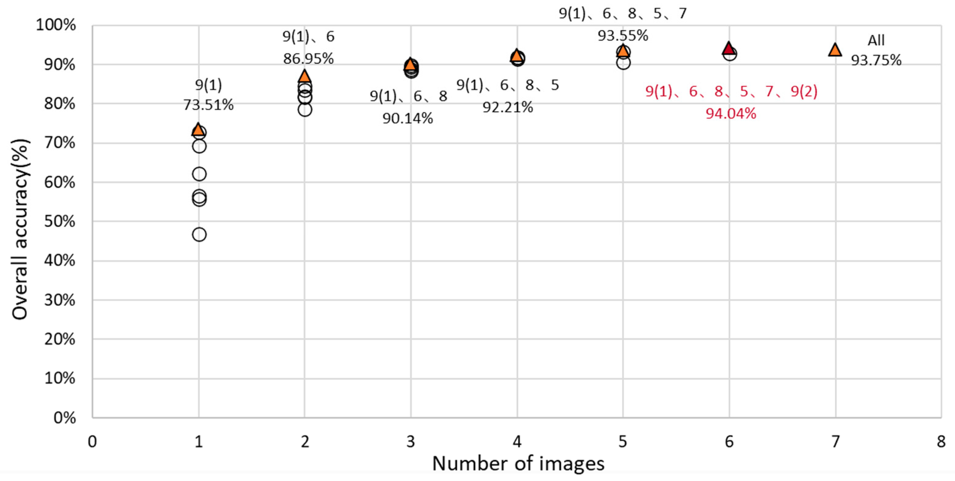
3.2.4. Optimal Combination of SAR Images and Polarimetric Observables

The corresponding accuracy assessments using single-date image (i.e., first step) with optimal combination of polarimetric observables are listed in

Table 7. Accuracy assessment of RF classifications with optimal combination of polarimetric observables using single SAR image on each date.

Acquisition Date	OA (%)	Kappa
12 April 2015	46.72	0.32
6 May 2015	55.66	0.45
23 June 2015	72.68	0.65
17 July 2015	62.14	0.51
10 August 2015	56.57	0.45
3 September 2015	73.51	0.66
27 September 2015	69.29	0.61

. SAR images in June and September still produced more accurate results. The selected optimal combination in the first step was still using the image on 3 September. Figure 13 shows the RF OA for the optimal combination produced by the forward image selection procedure using optimal combination of polarimetric observables. Similar to the previous tests, the most important acquisitions corresponded to summer and autumn (from June to September). The best OA was achieved using six images (in May, June, July, August, and September), with an OA of 94.04%, which was the highest value among all classification tests in this study. The corresponding classification map is given in Figure 14, which corresponds to the best crop classification performance over the study area in this research. It suggests that the combined use of optimal combination of polarimetric observables and acquisition dates may produce the best crop classification performance.

3.2.5. Sensitivity to Training and Testing Samples on Overall Classification Performance

By swapping the training and testing samples in Table 2, the accuracies of RF classifications with all polarimetric observables using a single SAR image on each date are listed in

Table 8. Accuracy assessment of RF classifications with all polarimetric observables using single SAR image on each date after exchanging the training and testing samples in previous tests.

Acquisition Date	OA (%)	Kappa
12 April 2015	55.25	0.45
6 May 2015	56.85	0.47
23 June 2015	68.12	0.61
17 July 2015	59.78	0.51
10 August 2015	55.30	0.45
3 September 2015	63.74	0.56
27 September 2015	67.49	0.60

. SAR images in June and September still produced the most accurate results, as in previous tests. Figure 15 shows the RF overall accuracies for the optimal combination of SAR images produced by a forward image selection procedure using all polarimetric observables. The optimal combination with the best accuracy used five images, in which four images were the same as before. This indicates, again, that fewer images on some critical dates may produce better accuracies.

3.2.6. Normalized Variable Importance for Crop Classification

Based on the unique ability of the RF algorithm, the variable importance for crop classification with all SAR images and all polarimetric observables was quantified across input features, as well as over all dates. Among the 189 variables (a total of seven images and 27 features for each image) used in the RF classification, the most important 50 variables are listed in ascending order in Figure 16. The variables from LP, Pauli, and Span exhibited the greatest importance, and the variables from polarimetric decompositions (FD, CP, ND) presented moderate importance in this study. Across time, generally the summer and autumn acquisitions (from June to September) occupied greater importance positions than the spring acquisitions (April and May).

4. Discussion

4.1. Temporal Evolutions of Polarimetric Observables

For crop growth monitoring, temporal evolutions of all 27 polarimetric observables extracted from the multi-temporal RADARSAT-2 data for different crop types were analyzed. The backscattering coefficients in cross-pol (HV), Pauli second channel (HH-VV), and HV/VV ratio were found to be the most sensitive observables to crop growth. The reason can be attributed to the sensitivity of these parameters to crop structure and its associated scattering mechanisms. The results are in line with previous studies [10,26,27]. The crop structural features were also well characterized by their unique scattering patterns using parameters derived from polarimetric decompositions (i.e., FD, CP, and ND). The difference in temporal evolution patterns of scattering mechanisms among crops provided useful information for crop classification, which have been frequently used in crop growth monitoring and classification in previous reports [7,17,27,38,39,41]. Among the polarimetric complex correlation parameters, the correlation coefficient ${\mathsf{\rho }}_{\mathrm{HHVV}}$ showed the highest sensitivity to crop growth, which has been proven useful for identification of growth stages [31,36]. The RVI also varied dramatically following the course of crop development, which has been successfully introduced for crop growth monitoring with full, dual and compact polarimetric SAR data [21,51,59].

4.2. Crop Classification

The results using single groups of polarimetric observables showed that polarimetric decompositions (ND, FD, and CP), backscattering coefficients in Pauli and linear polarimetric channels, and correlation coefficients produced the best classification accuracies, with OAs greater than 87%. This is because these polarimetric observables were found to be very sensitive to crop structure and growth parameters [7,17,27,38,39,41]. In previous studies, the common way for constructing the feature set was by stacking all polarimetric observables from various sources [7,17,27,39]. However, in our case, the classifications using an optimal combination of polarimetric observables with reduced number of polarimetric observables, i.e., eight groups (NM, FD, Ra, Pha, Ro, CP, RVI and Pauli), produced better overall accuracies for crop classification. Fewer images acquired on certain critical dates could produce better overall accuracies for crop classification, which is consistent with previous studies [10,27]. The best combination of SAR images was selected from the SAR dataset by the forward selection procedure, rather than combinations by adding images one by one sequentially along the SAR acquisition time as in previous reports [39,40]. The best result was achieved using an optimal combination of polarimetric observables and SAR images (including eight groups and six images), with an OA of 94.04%. This indicates that this strategy (a forward selection procedure for deciding the optimal combination of polarimetric observables and SAR images) is recommended for practical classification in operational scenarios.

4.3. Limitations and Future Research

There are some limitations in our study. First, the results were obtained specifically based on the C-band FQ10W RADARSAT-2 dataset over an agricultural area in South-western Ontario, Canada. Although radar signals are affected by both the sensor configurations (radar frequency, incidence angle, look direction) and the targets (crop mixture in different ecoregions), the information used for separating the targets stays the same. As long as there are structural differences and varying growth patterns among different crop types, the multitemporal SAR-based methodology presented in this study can be applied to crop classifications under different climate scenarios, and the classification accuracy will fluctuate depending on the complexity of the crop mix. Second, it is known that applying masks of noncropland land cover types could be helpful in reducing commission errors in the resulting crop classification map. However, a current and accurate cropland mask does not always exist and, therefore, we carried out the land cover classification in an agricultural site without that mask.

Future work will focus on crop growth monitoring and crop classification with PolSAR data at other radar frequencies (such as TerraSAR-X at X band, ALOS-2 at L band) and over different agricultural sites. Moreover, the forward selection procedure is helpful for investigating which type of features (time or polarimetric information) can contribute more to land-cover classification. For instance, the well-used and freely accessible Sentinel-1 data can only provide a dual-pol mode but with high temporal resolution (only six days for the two-satellite constellation). In addition, temporal variation of interferometric coherence has shown great potential in monitoring dynamics of the surface properties [60,61,62], which needs further investigation for crop monitoring and classification.

5. Conclusions

This study presents a comprehensive evaluation and demonstration of crop growth monitoring and crop type classification over an agricultural area in Southwestern Ontario, Canada, based on time series of polarimetric RADARSAT-2 C-band images acquired in the same beam mode across the full growing season. A set of 27 representative polarimetric observables was selected and analyzed. Temporal evolution studies showed that the backscattering coefficients in cross-pol (HV), Pauli second channel (HH-VV), and HV/VV ratio, polarimetric decomposition parameters, RVI were found to be the most sensitive observables to crop growth. By using the well-known Random Forest (RF) algorithm, the classification results using single groups of polarimetric observables showed that polarimetric decomposition methods (ND, FD, and CP), backscattering coefficients in Pauli and linear polarimetric channels and correlation coefficients produced the best classification accuracies, with OAs greater than 87%. The forward selection procedure for pursuing optimal classification accuracy from different perspectives was expanded to find optimal combinations of polarimetric observables, or SAR images, or both. The results showed that fewer polarimetric observables, or fewer images on certain critical dates, could produce better overall accuracies for crop classification. The best result was achieved using an optimal combination of polarimetric observables and SAR images (including eight groups and six images), with an OA of 94.04%. This suggests that an optimal combination considering both perspectives (i.e., numbers of images and polarimetric observables) is valuable and could serve as a guideline, which is transferable for crop classification in practice.

References

1. Brown, L.R. Outgrowing the Earth: The Food Security Challenge in an Age of Falling Water Tables and Rising Temperatures; W. W. Norton & Company: New York, NY, USA, 2005. [Google Scholar]
2. Liu, C.; Chen, Z.; Shao, Y.; Chen, J.; Hasi, T.; Pan, H. Research advances of SAR remote sensing for agriculture applications: A review. J. Integr. Agric. 2019, 18, 506–525. [Google Scholar] [CrossRef] [Green Version]
3. McNairn, H.; Shang, J.; Jiao, X.; Champagne, C. The contribution of ALOS PALSAR multipolarization and polarimetric data to crop classification. IEEE Trans. Geosci. Remote Sens. 2009, 47, 3981–3992. [Google Scholar] [CrossRef] [Green Version]
4. Thenkabail, P.S.; Knox, J.W.; Ozdogan, M.; Gumma, M.K.; Congalton, R.G.; Wu, Z.; Milesi, C.; Finkral, A.; Marshall, M.; Mariotto, I.; et al. Assessing future risks to agricultural productivity, water resources and food security: How can remote sensing help? Photogramm. Eng. Remote Sens. 2012, 78, 773–782. [Google Scholar]
5. Bargiel, D. A new method for crop classification combining time series of radar images and crop phenology information. Remote Sens. Environ. 2017, 198, 369–383. [Google Scholar] [CrossRef]
6. Yang, J.; Yang, S.; Zhang, Y.; Shi, S.; Du, L. Improving characteristic band selection in leaf biochemical property estimation considering interrelations among biochemical parameters based on the PROSPECT-D model. Opt. Express 2021, 29, 400. [Google Scholar] [CrossRef]
7. Li, H.; Zhang, C.; Zhang, S.; Atkinson, P.M. Crop classification from full-year fully-polarimetric L-band UAVSAR time-series using the Random Forest algorithm. Int. J. Appl. Earth Obs. Geoinf. 2020, 87, 102032. [Google Scholar] [CrossRef]
8. Ozdogan, M.; Woodcock, C.E. Resolution dependent errors in remote sensing of cultivated areas. Remote Sens. Environ. 2006, 103, 203–217. [Google Scholar] [CrossRef]
9. Wardlow, B.D.; Egbert, S.L. Large-area crop mapping using time-series MODIS 250 m NDVI data: An assessment for the U.S. central great plains. Remote Sens. Environ. 2008, 112, 1096–1116. [Google Scholar] [CrossRef]
10. Jiao, X.; Kovacs, J.M.; Shang, J.; McNairn, H.; Walters, D.; Ma, B.; Geng, X. Object-oriented crop mapping and monitoring using multi-temporal polarimetric RADARSAT-2 data. ISPRS J. Photogramm. Remote Sens. 2014, 96, 38–46. [Google Scholar] [CrossRef]
11. Wang, K.; Franklin, S.E.; Guo, X.; He, Y.; McDermid, G.J. Problems in remote sensing of landscapes and habitats. Prog. Phys. Geogr. Earth Environ. 2009, 33, 747–768. [Google Scholar] [CrossRef] [Green Version]
12. Blaes, X.; Vanhalle, L.; Defourny, P. Efficiency of crop identification based on optical and SAR image time series. Remote Sens. Environ. 2005, 96, 352–365. [Google Scholar] [CrossRef]
13. Dong, J.; Xiao, X.; Kou, W.; Qin, Y.; Zhang, G.; Li, L.; Jin, C.; Zhou, Y.; Wang, J.; Biradar, C.; et al. Tracking the dynamics of paddy rice planting area in 1986–2010 through time series Landsat images and phenology-based algorithms. Remote Sens. Environ. 2015, 160, 99–113. [Google Scholar] [CrossRef]
14. Skakun, S.; Kussul, N.; Shelestov, A.Y.; Lavreniuk, M.; Kussul, O. Efficiency assessment of multitemporal C-band RADARSAT-2 intensity and landsat-8 surface reflectance satellite imagery for crop classification in Ukraine. IEEE J. Sel. Top. Appl. Earth Obs. Remote Sens. 2016, 9, 3712–3719. [Google Scholar] [CrossRef]
15. Liu, C.; Shang, J.; Vachon, P.W.; McNairn, H. Multiyear crop monitoring using polarimetric RADARSAT-2 data. IEEE Trans. Geosci. Remote Sens. 2013, 51, 2227–2240. [Google Scholar] [CrossRef]
16. Steele-Dunne, S.C.; McNairn, H.; Monsivais-Huertero, A.; Judge, J.; Liu, P.W.; Papathanassiou, K. Radar remote sensing of agricultural canopies: A Review. IEEE J. Sel. Top. Appl. Earth Obs. Remote Sens. 2017, 10, 2249–2273. [Google Scholar] [CrossRef] [Green Version]
17. Liao, C.; Wang, J.; Xie, Q.; Baz, A.A.; Huang, X.; Shang, J.; He, Y. Synergistic Use of multi-temporal RADARSAT-2 and VENµS data for crop classification based on 1D convolutional neural network. Remote Sens. 2020, 12, 832. [Google Scholar] [CrossRef] [Green Version]
18. Alonso-Gonzalez, A.; Lopez-Martinez, C.; Papathanassiou, K.P.; Hajnsek, I. Polarimetric SAR time series change analysis over agricultural areas. IEEE Trans. Geosci. Remote Sens. 2020, 58, 7317–7330. [Google Scholar] [CrossRef]
19. Larrañaga, A.; Álvarez-Mozos, J. On the added value of quad-pol data in a multi-temporal crop classification framework based on RADARSAT-2 imagery. Remote Sens. 2016, 8, 335. [Google Scholar] [CrossRef] [Green Version]
20. Huang, X.; Wang, J.; Shang, J.; Liao, C.; Liu, J. Application of polarization signature to land cover scattering mechanism analysis and classification using multi-temporal C-band polarimetric RADARSAT-2 imagery. Remote Sens. Environ. 2017, 193, 11–28. [Google Scholar] [CrossRef]
21. Mandal, D.; Kumar, V.; Ratha, D.; Dey, S.; Bhattacharya, A.; Lopez-Sanchez, J.M.; McNairn, H.; Rao, Y.S. Dual polarimetric radar vegetation index for crop growth monitoring using sentinel-1 SAR data. Remote Sens. Environ. 2020, 247, 111954. [Google Scholar] [CrossRef]
22. Homayouni, S.; McNairn, H.; Hosseini, M.; Jiao, X.; Powers, J. Quad and compact multitemporal C-band PolSAR observations for crop characterization and monitoring. Int. J. Appl. Earth Obs. Geoinf. 2019, 74, 78–87. [Google Scholar] [CrossRef]
23. Xu, L.; Zhang, H.; Wang, C.; Zhang, B.; Liu, M. Crop classification based on temporal information using sentinel-1 SAR time-series data. Remote Sens. 2018, 11, 53. [Google Scholar] [CrossRef] [Green Version]
24. Vicente-Guijalba, F.; Martinez-Marin, T.; Lopez-Sanchez, J.M. Dynamical approach for real-time monitoring of agricultural crops. IEEE Trans. Geosci. Remote Sens. 2015, 53, 3278–3293. [Google Scholar] [CrossRef] [Green Version]
25. Lopez-Sanchez, J.M.; Ballester-Berman, J.D.; Hajnsek, I.; Hajnsek, I. First results of rice monitoring practices in Spain by means of time series of TerraSAR-X Dual-Pol Images. IEEE J. Sel. Top. Appl. Earth Obs. Remote Sens. 2011, 4, 412–422. [Google Scholar] [CrossRef]
26. Canisius, F.; Shang, J.; Liu, J.; Huang, X.; Ma, B.; Jiao, X.; Geng, X.; Kovacs, J.M.; Walters, D. Tracking crop phenological development using multi-temporal polarimetric RADARSAT-2 data. Remote Sens. Environ. 2018, 210, 508–518. [Google Scholar] [CrossRef]
27. Li, H.; Zhang, C.; Zhang, S.; Atkinson, P.M. Full year crop monitoring and separability assessment with fully-polarimetric L-band UAVSAR: A case study in the Sacramento Valley, California. Int. J. Appl. Earth Obs. Geoinf. 2019, 74, 45–56. [Google Scholar] [CrossRef] [Green Version]
28. Cloude, S.R. Polarisation: Applications in Remote Sensing Polarisation; Oxford University Press: New York, NY, USA, 2010; ISBN 978-0-19-956973-1. [Google Scholar]
29. Lee, J.; Pottier, E. Polarimetric Radar Imaging: From basics to applications; CRC Press: Boca Raton, FL, USA, 2009; ISBN 142005497X. [Google Scholar]
30. Lin, Y.C.; Sarabandi, K. A Monte Carlo coherent scattering model for forest canopies using fractal-generated trees. IEEE Trans. Geosci. Remote Sens. 1999, 37, 440–451. [Google Scholar] [CrossRef]
31. Lopez-Sanchez, J.M.; Cloude, S.R.; Ballester-Berman, J.D. Rice phenology monitoring by means of SAR polarimetry at X-band. IEEE Trans. Geosci. Remote Sens. 2012, 50, 2695–2709. [Google Scholar] [CrossRef]
32. Lopez-Sanchez, J.M.; Vicente-Guijalba, F.; Ballester-Berman, J.D.; Cloude, S.R. Polarimetric response of rice fields at C-band: Analysis and phenology retrieval. IEEE Trans. Geosci. Remote Sens. 2014, 52, 2977–2993. [Google Scholar] [CrossRef] [Green Version]
33. Busquier, M.; Lopez-Sanchez, J.M.; Mestre-Quereda, A.; Navarro, E.; González-Dugo, M.P.; Mateos, L. Exploring TanDEM-X interferometric products for crop-type mapping. Remote Sens. 2020, 12, 1774. [Google Scholar] [CrossRef]
34. Busquier, M.; Lopez-Sanchez, J.M.; Bargiel, D. Added value of coherent copolar polarimetry at X-band for crop-type mapping. IEEE Geosci. Remote Sens. Lett. 2020, 17, 819–823. [Google Scholar] [CrossRef]
35. Xu, S.; Qi, Z.; Li, X.; Yeh, A.G.-O. Investigation of the effect of the incidence angle on land cover classification using fully polarimetric SAR images. Int. J. Remote Sens. 2019, 40, 1576–1593. [Google Scholar] [CrossRef]
36. Lopez-Sanchez, J.M.; Vicente-Guijalba, F.; Ballester-Berman, J.D.; Cloude, S.R. Influence of incidence angle on the coherent copolar polarimetric response of rice at X-band. IEEE Geosci. Remote Sens. Lett. 2015, 12, 249–253. [Google Scholar] [CrossRef] [Green Version]
37. Valcarce-Diñeiro, R.; Lopez-Sanchez, J.M.; Sánchez, N.; Arias-Pérez, B.; Martínez-Fernández, J. Influence of incidence angle in the correlation of C-band polarimetric parameters with biophysical variables of rain-fed crops. Can. J. Remote Sens. 2019, 44, 643–659. [Google Scholar] [CrossRef]
38. Xie, Q.; Wang, J.; Lopez-Sanchez, J.M.; Peng, X.; Liao, C.; Shang, J.; Zhu, J.; Fu, H.; Ballester-Berman, J.D. Crop height estimation of corn from multi-year RADARSAT-2 polarimetric observables using machine learning. Remote Sens. 2021, 13, 392. [Google Scholar] [CrossRef]
39. Liao, C.; Wang, J.; Huang, X.; Shang, J. Contribution of minimum noise fraction transformation of multi-temporal RADARSAT-2 polarimetric SAR data to cropland classification. Can. J. Remote Sens. 2018, 44, 215–231. [Google Scholar] [CrossRef]
40. Xie, Y.; Fu, H.; Zhu, J.; Wang, C.; Xie, Q. A LiDAR-aided multibaseline polInSAR method for forest height estimation: With emphasis on dual-baseline selection. IEEE Geosci. Remote Sens. Lett. 2020, 17, 1807–1811. [Google Scholar] [CrossRef]
41. Xie, Q.; Wang, J.; Liao, C.; Shang, J.; Lopez-Sanchez, J.M.; Fu, H.; Liu, X. On the use of Neumann decomposition for crop classification using multi-temporal RADARSAT-2 polarimetric SAR data. Remote Sens. 2019, 11, 776. [Google Scholar] [CrossRef] [Green Version]
42. Jiao, X.; Mc Nairn, H.; Shang, J.; Pattey, E.; Liu, J.; Champagne, C. The sensitivity of RADARSAT-2 polarimetric SAR data to corn and soybean leaf area index. Can. J. Remote Sens. 2011, 37, 69–81. [Google Scholar] [CrossRef]
43. Erten, E.; Taskin, G.; Lopez-Sanchez, J.M. Selection of PolSAR observables for crop biophysical variable estimation with global sensitivity analysis. IEEE Geosci. Remote Sens. Lett. 2019, 13, 1–5. [Google Scholar] [CrossRef]
44. Liao, C.; Wang, J.; Shang, J.; Huang, X.; Liu, J.; Huffman, T. Sensitivity study of RADARSAT-2 polarimetric SAR to crop height and fractional vegetation cover of corn and wheat. Int. J. Remote Sens. 2018, 39, 1475–1490. [Google Scholar] [CrossRef]
45. Touzi, R.; Lopes, A.; Bruniquel, J.; Vachon, P.W. Coherence estimation for SAR imagery. IEEE Trans. Geosci. Remote Sens. 1999, 37, 135–149. [Google Scholar] [CrossRef] [Green Version]
46. Freeman, A.; Durden, S.L. A three-component scattering model for polarimetric SAR data. IEEE Trans. Geosci. Remote Sens. 1998, 36, 963–973. [Google Scholar] [CrossRef] [Green Version]
47. Cloude, S.R.; Pottier, E. An entropy based classification scheme for land applications of polarimetric SAR. IEEE Trans. Geosci. Remote Sens. 1997, 35, 68–78. [Google Scholar] [CrossRef]
48. Neumann, M.; Ferro-Famil, L.; Jager, M.; Reigber, A.; Pottier, E. A Polarimetric Vegetation Model to Retrieve Particle and Orientation Distribution Characteristics. In Proceedings of the 2009 IEEE International Geoscience and Remote Sensing Symposium, Cape Town, South Africa, 12–17 July 2009; Volume 4, pp. IV-145–IV-148. [Google Scholar]
49. Kim, Y.; van Zyl, J. Comparison of Forest Parameter Estimation Techniques Using SAR data. In Proceedings of the IGARSS 2001. Scanning the Present and Resolving the Future. IEEE 2001 International Geoscience and Remote Sensing Symposium (Cat. No.01CH37217), Sydney, NSW, Australia, 9–13 July 2001; Volume 3, pp. 1395–1397. [Google Scholar]
50. Kim, Y.; van Zyl, J. A time-series approach to estimate soil moisture using polarimetric radar data. IEEE Trans. Geosci. Remote Sens. 2009, 47, 2519–2527. [Google Scholar] [CrossRef]
51. Ratha, D.; Mandal, D.; Kumar, V.; McNairn, H.; Bhattacharya, A.; Frery, A.C. A generalized volume scattering model-based vegetation index from polarimetric SAR data. IEEE Geosci. Remote Sens. Lett. 2019, 10, 1–5. [Google Scholar] [CrossRef]
52. Kim, Y.; Jackson, T.; Bindlish, R.; Hong, S.; Jung, G.; Lee, K. Retrieval of wheat growth parameters with radar vegetation indices. IEEE Geosci. Remote Sens. Lett. 2014, 11, 808–812. [Google Scholar] [CrossRef]
53. Arii, M.; van Zyl, J.J.; Kim, Y. A general characterization for polarimetric scattering from vegetation canopies. IEEE Trans. Geosci. Remote Sens. 2010, 48, 3349–3357. [Google Scholar] [CrossRef]
54. Deschamps, B.; McNairn, H.; Shang, J.; Jiao, X. Towards operational radar-only crop type classification: Comparison of a traditional decision tree with a random forest classifier. Can. J. Remote Sens. 2012, 38, 60–68. [Google Scholar] [CrossRef]
55. Sonobe, R.; Tani, H.; Wang, X.; Kobayashi, N.; Shimamura, H. Random forest classification of crop type using multi-temporal TerraSAR-X dual-polarimetric data. Remote Sens. Lett. 2014, 5, 157–164. [Google Scholar] [CrossRef] [Green Version]
56. Hariharan, S.; Mandal, D.; Tirodkar, S.; Kumar, V.; Bhattacharya, A.; Lopez-Sanchez, J.M. A novel phenology based feature subset selection technique using random forest for multitemporal PolSAR crop classification. IEEE J. Sel. Top. Appl. Earth Obs. Remote Sens. 2018, 11, 4244–4258. [Google Scholar] [CrossRef] [Green Version]
57. Breiman, L. Random forest. Mach. Learn. 2001, 45, 5–32. [Google Scholar] [CrossRef] [Green Version]
58. Pal, M. Random forest classifier for remote sensing classification. Int. J. Remote Sens. 2005, 26, 217–222. [Google Scholar] [CrossRef]
59. Mandal, D.; Ratha, D.; Bhattacharya, A.; Kumar, V.; McNairn, H.; Rao, Y.S.; Frery, A.C. A radar vegetation index for crop monitoring using compact polarimetric SAR data. IEEE Trans. Geosci. Remote Sens. 2020, 58, 6321–6335. [Google Scholar] [CrossRef]
60. Mestre-Quereda, A.; Lopez-Sanchez, J.M.; Vicente-Guijalba, F.; Jacob, A.W.; Engdahl, M.E. Time-Series of Sentinel-1 Interferometric Coherence and Backscatter for Crop-Type Mapping. IEEE J. Sel. Top. Appl. Earth Obs. Remote Sens. 2020, 13, 4070–4084. [Google Scholar] [CrossRef]
61. Jacob, A.W.; Vicente-Guijalba, F.; Lopez-Martinez, C.; Lopez-Sanchez, J.M.; Litzinger, M.; Kristen, H.; Mestre-Quereda, A.; Ziolkowski, D.; Lavalle, M.; Notarnicola, C.; et al. Sentinel-1 InSAR Coherence for Land Cover Mapping: A Comparison of Multiple Feature-Based Classifiers. IEEE J. Sel. Top. Appl. Earth Obs. Remote Sens. 2020, 13, 535–552. [Google Scholar] [CrossRef] [Green Version]
62. Zhang, Z.; Wang, C.; Zhang, H.; Tang, Y.; Liu, X. Analysis of Permafrost Region Coherence Variation in the Qinghai–Tibet Plateau with a High-Resolution TerraSAR-X Image. Remote Sens. 2018, 10, 298. [Google Scholar] [CrossRef] [Green Version]
Figure 1. Location and Pauli RGB image acquired on 12 April 2015 over the overlapping area of all RADARSAT-2 images. (RADARSAT-2 Data and Products © MacDonald, Dettwiler and Associates Ltd. (2015)—All Rights Reserved. RADARSAT is an official trademark of the Canadian Space Agency).
Remotesensing 13 01394 g001
Figure 2. Field photos of three main crop types over the study site on selected acquisition dates. Top row, winter wheat; middle row, corn; bottom row, soybean. The grey boxes correspond to no photos taken due to crop fields in preparation, seeding or harvested time.
Remotesensing 13 01394 g002aRemotesensing 13 01394 g002b
Figure 3. Field photos of three main crop types over the study site on 23 May when the field survey for corn and soybean fields started.
Remotesensing 13 01394 g003
Figure 4. Map of ground truth of the study site from field survey by the Geographic Information Technology and Application (GITA) Lab, UWO in 2015.
Remotesensing 13 01394 g004
Figure 5. Temporal evolutions in synthetic aperture radar (SAR) backscattering. (a) HH; (b) HV; (c) VV; (d) HH + VV; (e) HH-VV; (f) Span; (g) HH/VV; (h) HV/VV; (i) HV/HH. Note error bars denote standard deviation.
Remotesensing 13 01394 g005aRemotesensing 13 01394 g005b
Figure 6. Temporal evolutions of polarimetric decomposition parameters for different crops. (a) surface scattering (Ps); (b) double-bounce scattering (Pd); (c) volume scattering (Pv); (d) entropy (H); (e) alpha angle (α); (f) anisotropy (A); (g) degree of orientation randomness (τ); (h) magnitude of the particle scattering anisotropy | δ | ; (i) phase of the particle scattering anisotropy   ϕ δ . Note error bars denote standard deviation.
Remotesensing 13 01394 g006aRemotesensing 13 01394 g006b
Figure 7. Temporal evolutions in correlation coefficients, phase differences and radar vegetation indexes (RVIs) for crops. (a) ρ H H V V ; (b) ρ H V V V ; (c) ρ H H H V ; (d) ρ H H + V V , H H V V ; (e) ϕ H H V V ; (f) ϕ H V V V ; (g) ϕ H H H V ; (h) ϕ H H + V V , H H V V . Note error bars denote standard deviation.
Remotesensing 13 01394 g007aRemotesensing 13 01394 g007b
Figure 8. Temporal evolutions in RVI. Note error bars denote standard deviation.
Remotesensing 13 01394 g008
Figure 9. Classification maps with all RADARSAT-2 images and Random Forest algorithm using different groups of polarimetric observables. (a) LP; (b) Pauli; (c) Span; (d) Ra; (e) Ro; (f) Pha; (g) FD; (h) CP; (i) ND; (j) RVI.
Remotesensing 13 01394 g009
Figure 10. The RF overall accuracies for the optimal combination of polarimetric observables produced by a forward feature selection procedure using all multitemporal RADARSAT-2 images. Note that numbers in the figure denote the best accuracy in each step, and the abbreviations are explained in Table 3.
Remotesensing 13 01394 g010
Figure 11. Classification map with the best accuracy using an optimal combination of polarimetric observables from all RADARSAT-2 images (OA = 93.75%).
Remotesensing 13 01394 g011
Figure 12. The RF overall accuracies for the optimal combination SAR image produced by a forward image selection procedure using all polarimetric observables. Note that numbers in the figure denote the best accuracy in each step (at the bottom), and combinations of SAR images (at the top), for example “9(1), 6, 8, 9(2)” represents the combination of images dated 3 September, 23 June, 10 August and 27 September (see Table 1).
Remotesensing 13 01394 g012
Figure 13. The RF overall accuracies for the optimal combination SAR image produced by a forward image selection procedure using optimal combination of polarimetric observables. Note that numbers in the figure denote the best accuracy in each step (at the bottom), and combinations of SAR images (at the top), for example “9(1), 6, 8, 5” represents the combination of images dated 3 September, 23 June, 10 August and 6 May (see Table 1).
Remotesensing 13 01394 g013
Figure 14. Classification map with the best accuracy simultaneously using optimal combination of polarimetric observables and images (OA = 94.04%).
Remotesensing 13 01394 g014
Figure 15. The RF overall accuracies for the optimal combination SAR image produced by a forward image selection procedure using all polarimetric observables after exchanging the training and testing samples in previous tests. Note that numbers in the figure denote the best accuracy in each step (at the bottom), and combinations of SAR images (at the top), for example “6, 9(1), 5, 8, 4” represents the combination of images dated 23 June, 3 September, 6 May, 10 August, and 12 April (see Table 1).
Remotesensing 13 01394 g015
Figure 16. Normalized variable importance of RF classification with all polarimetric observables using all RADARSAT-2 images. Different types of polarimetric variables are represented as follows: LP (purple), Pauli (dark green), Span (light green), Ra (blue); Ro (orange), Pha (green), FD (pink), CP (yellow), ND (red), RVI (cyan). A variable name consists of three parts, with the prefix, center, and suffix respectively representing acquisition date, date source (see Table 1), and a certain variable (none if only one variable from data source, such as Span and RVI). For example, the first variable name 0927-Pauli-HH-VV represents the backscattering coefficient HH-VV from Pauli channel using SAR image on 27 September.
Remotesensing 13 01394 g016