Urban Heat Island Formation in Greater Cairo: Spatio-Temporal Analysis of Daytime and Nighttime Land Surface Temperatures along the Urban–Rural Gradient

Abstract

An urban heat island (UHI) is a significant anthropogenic modification of urban land surfaces, and its geospatial pattern can increase the intensity of the heatwave effects. The complex mechanisms and interactivity of the land surface temperature in urban areas are still being examined. The urban–rural gradient analysis serves as a unique natural opportunity to identify and mitigate ecological worsening. Using Landsat Thematic Mapper (TM), Operational Land Imager/Thermal Infrared Sensor (OLI/TIRS) and Moderate Resolution Imaging Spectroradiometer (MODIS), Land Surface Temperature (LST) data in 2000, 2010, and 2019, we examined the spatial difference in daytime and nighttime LST trends along the urban–rural gradient in Greater Cairo, Egypt. Google Earth Engine (GEE) and machine learning techniques were employed to conduct the spatio-temporal analysis. The analysis results revealed that impervious surfaces (ISs) increased significantly from 564.14 km² in 2000 to 869.35 km² in 2019 in Greater Cairo. The size, aggregation, and complexity of patches of ISs, green space (GS), and bare land (BL) showed a strong correlation with the mean LST. The average urban–rural difference in mean LST was −3.59 °C in the daytime and 2.33 °C in the nighttime. In the daytime, Greater Cairo displayed the cool island effect, but in the nighttime, it showed the urban heat island effect. We estimated that dynamic human activities based on the urban structure are causing the spatial difference in the LST distribution between the day and night. The urban–rural gradient analysis indicated that this phenomenon became stronger from 2000 to 2019. Considering the drastic changes in the spatial patterns and the density of IS, GS, and BL, urban planners are urged to take immediate steps to mitigate increasing surface UHI; otherwise, urban dwellers might suffer from the severe effects of heatwaves.

1. Introduction

Urbanization impairs the natural landscape as it produces impervious surfaces. Rapid urbanization has become one of the most critical global issues in the 21st century [1,2,3,4]. Various socio-environmental problems, including climate change [5,6,7], energy systems [8], deforestation [9], water and air quality [10], and environmental health [11], have been attributed to large regions being urbanized too rapidly and without proper planning.

The urban heat island (UHI) phenomenon [12,13,14,15], which refers to higher temperatures in urban areas relative to the surroundings, has been studied in many cities around the world [15,16,17,18,19]. The distribution of impervious surfaces covered by cement, asphalt, and concrete raises the land’s radiative surface temperature [20] and changes the humidity of urban areas [21,22]. The rise in heat in urban areas has caused various social problems such as increasing water and energy consumption [23], air pollution [24], discomfort, and human health issues like cardiovascular disease and psychological stress [25,26]. Hence, a better understanding of the UHI mechanism is crucial for planning its effective mitigation and adaptive strategies for urban sustainability [20,27,28,29].

We can classify UHI into two types: atmospheric urban heat islands and surface urban heat islands [16,30]. The former considers the UHI effects in the canopy or boundary layers [31,32], whereas the latter considers the surface difference in radiative temperature [33,34,35,36]. Generally, atmospheric urban heat islands are measured and modeled by in situ sensors (meteorological stations or towers), radiosondes, and aircraft [31,37]. Although the instruments provide more reliable air UHI readings, they are expensive to install [34]. As there are few global monitoring stations, air UHIs do not provide substantial measurements in the context of urban planning and climate change studies [31]. Hence, surface UHI plays a more significant role, with satellite-based surface UHI being applied for repeatable spatio-temporal measurements at local [34,38,39,40,41], regional [20,29,42,43,44,45], and global scales [46,47]. Surface UHI also plays an important role in thermal anisotropy [48]. The degree of surface UHI differs according to seasons, solar intensity, land cover, and weather [12]. Furthermore, surface UHIs widely differ between day and night [12]. Due to the sun’s radiation, daytime surface UHI is stronger than that of nighttime.

The concept of local climate zone(s) is one method for examining surface UHIs in the urban environments [49,50,51]. However, urban–rural gradient analysis has been widely used to investigate the geographical pattern of surface UHI. For instance, Estoque et al. [12] demonstrated the surface UHI effect in three megacities in Southeast Asia by combining urban–rural gradient analysis and spatial metrics-based analysis using Landsat imageries. Yang et al. [52] discussed the spatio-temporal vegetation pattern based on an urban–rural gradient in Dalian, China, using Moderate Resolution Imaging Spectroradiometer (MODIS data). Fu et al. [53] studied the variability in annual temperature cycles in the USA, also using MODIS data. Athukorala and Murayama [54] discussed the spatial variation in surface urban heat islands in Accra, Ghana, employing the urban–urban gradient and landscape-metrics-based analysis. Thus, many scholars have demonstrated that satellite data are useful for investigating the relationship between landscape patterns and LST [55,56,57].

Today, urban–rural gradient analysis and spatial configuration analysis based on spatial metrics [58,59] provide valuable insights into the progress in UHI studies as well as useful information on urban design and urban landscape planning [54,60]. However, there are relatively few studies on surface UHIs, especially in rapidly growing cities in Africa [61,62,63,64], including Cairo [65,66]. Therefore, we focused on Cairo (Egypt), one of Africa’s important megacities in this study because it has experienced drastic urbanization during the last two decades [67]. We examined the spatial relationship between surface UHI and the urban–rural gradient for Greater Cairo in 2000, 2010, and 2019 using Moderate Resolution Imaging Spectroradiometer (MODIS), land surface temperature (LST) products. We used Landsat imageries to identify the spatio-temporal changes in land use/cover (LUC) in Greater Cairo and to understand the relationship between LST and the LUC categories of the study area.

The objectives of this study were to (1) investigate urban LUC changes, (2) examine surface UHI and the urban–rural gradient, and (3) discuss the spatial relationship between the surface UHIs and the urban structure in Greater Cairo. Surface UHIs have been widely studied in tropical and temperate regions [68,69,70]. In contrast, understanding how urbanization is associated with the climate in the hot desert environment is still limited [71]. Both daytime and nighttime urban heat island studies in these kinds of cities are lacking. Unlike previous Cairo studies [65,72], we focused on land surface temperatures in both daytime and nighttime along the urban–rural gradient to deepen our understanding of urban dynamism within a day and gather critical information regarding climate change mitigation studies.

2. Materials and Methods

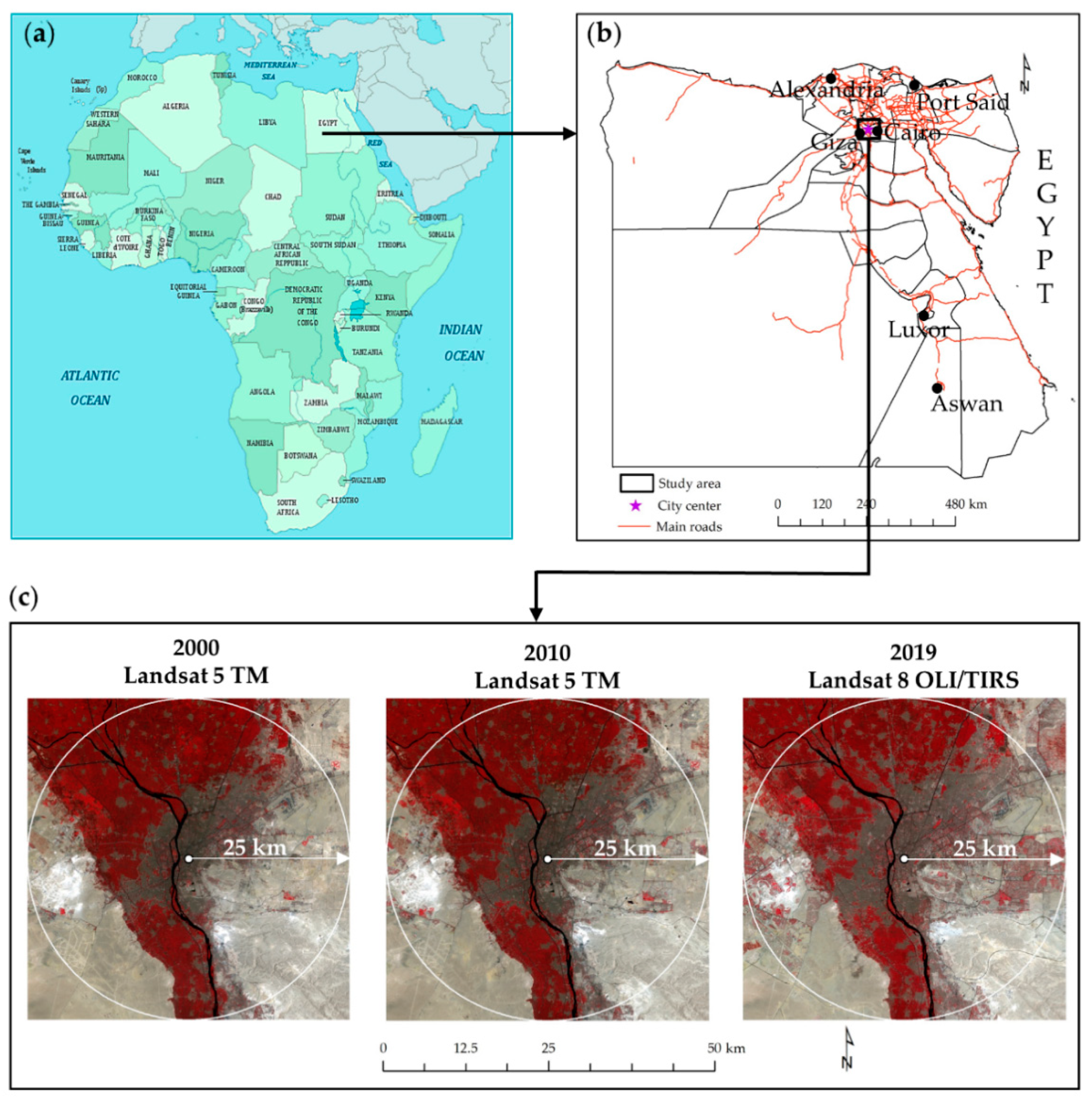
2.1. Study Area

Cairo, the capital of Egypt, is located at 30°060′ N and 31°28′ E, at 74.5 m above sea level (asl) in the Nile basin (Figure 1).Cairo has the longest history in the African continent [73]. Greater Cairo accounts for the most significant urban agglomeration in Africa and is eleventh in the world in this respect [72]. The study area stretches 50 $\times$ 50 km with a 25 km buffer from the city center. The city center is the urban core based on geographical and socio-economic significance (Figure 1).

Greater Cairo comprises three urban administrative divisions: Cairo, Giza, and Al-Qalubiya. The number of listed inhabitants reached 20 million in 2018, which is second only to Lagos, Nigeria, in Africa [74,75]. In Greater Cairo, there are barren desert and bare land in the eastern region and cultivated land in the Nile Delta and the Nile River to the west. Roads and streets in Greater Cairo are covered with asphalt, and other surfaces are covered mostly with desert sand. According to the Koppen climate classification, Greater Cairo, with relatively flat terrain, has a hot desert climate [75,76].

Climatologically, Greater Cairo belongs to the sub-tropical climatic region. Sandy winds are dominant from March to May (spring) and September to November (Autumn). December to February are the winter months, during which it is relatively humid, and there is little rain. Summer, from July to August, is hot, dry, and rainless. The annual rainfall in Greater Cairo is about 20 mm, and the average daily mean temperature is 19.7 °C in January and 34.9 °C in July [73].

Figure 1. Location of Greater Cairo: (a) Egypt and other African countries [77]; (b) Egypt and Greater Cairo [78]; and (c) study area with 25 km buffer from the city center in 2000, 2010, and 2019. False-color band composites in 2000, 2010, and 2019 were downloaded from the Google Earth Engine (GEE) platform [79].

Figure 1. Location of Greater Cairo: (a) Egypt and other African countries [77]; (b) Egypt and Greater Cairo [78]; and (c) study area with 25 km buffer from the city center in 2000, 2010, and 2019. False-color band composites in 2000, 2010, and 2019 were downloaded from the Google Earth Engine (GEE) platform [79].

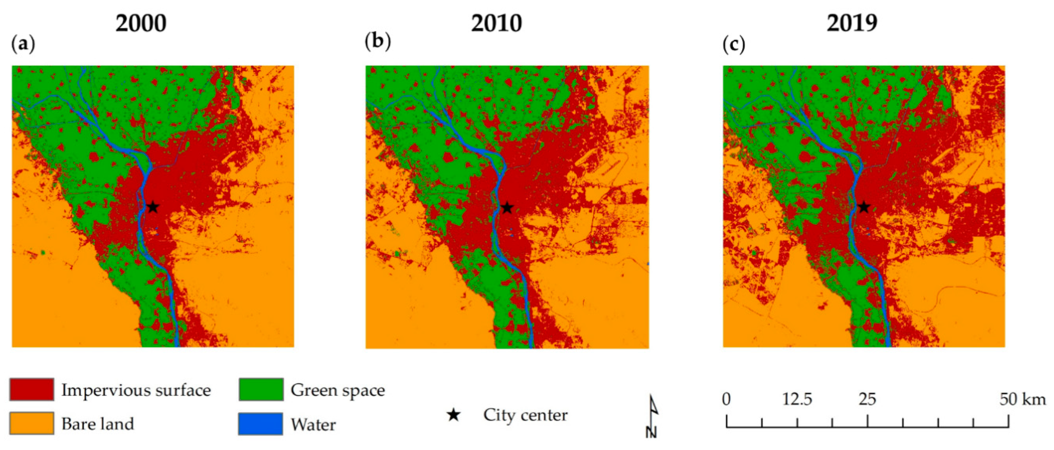
2.2. LUC Classification

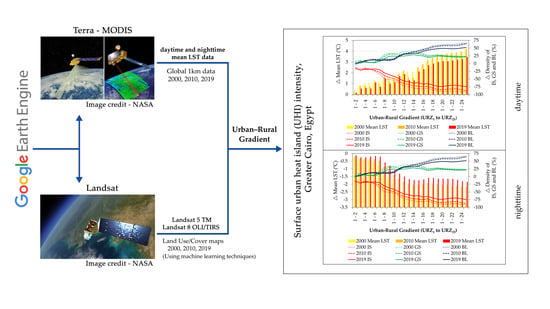
We downloaded the atmospherically corrected pre-processed (level 2) Landsat data from the GEE platform in 2000, 2010, and 2019 [79]. First, we demarcated the 50 $\times$ 50 km boundary for the study area and prepared the boundary shapefile. The city center is located in the central business district (CBD). Second, the boundary shapefile was imported on Asset in GEE. Finally, we ran the script for Greater Cairo to download Landsat imageries for summer (July and August). In this stage, we ran the script three times for three time points. Using the Image Collection tool in GEE, we prepared the three final Landsat imageries, including four images for 2000 (Landsat 5), two images for 2010 (Landsat 5), and four images for 2019 (Landsat 8) (Appendix A

Table A1. List of Landsat images used in this study (Level 2). TM, Thematic Matter; OLI/TIRS, Operational Land Imager/Thermal Infrared Sensor.

Year	Sensor	Image ID	Acquisition Date
2000	Landsat 5 TM	LT05_L2SP_176039_20000714_20200906_02_T1	14-07-2000
		LT05_L2SP_176039_20000730_20200906_02_T1	30-07-2000
		LT05_L2SP_176039_20000815_20200907_02_T1	15-08-2000
		LT05_L2SP_176039_20000831_20200907_02_T1	31-08-2000
2010	Landsat 5 TM	LT05_L2SP_176039_20100710_20200823_02_T1	10-07-2010
		LT05_L2SP_176039_20100710_20200823_02_T1	27-08-2010
2019	Landsat 8 OLI/TIRS	LC08_L2SP_176039_20190703_20200827_02_T1	03-07-2019
		LC08_L2SP_176039_20190719_20200827_02_T1	19-07-2019
		LC08_L2SP_176039_20190804_20200827_02_T1	04-08-2019
		LC08_L2SP_176039_20190820_20200827_02_T1	20-08-2019

) for Greater Cairo. All downloaded images were projected onto the WGS84/UTM 36N projection system before further processing.

The LUC maps of the study area were constructed by applying four machine learning methods: K-nearest neighbor (KNN), artificial neural network (ANN), support vector machine (SVM), and random forest (RF), facilitated by the R software [80]. In the LUC classification, bands 4, 3, and 2 for Landsat 5 and bands 5, 4, and 3 for Landsat 8 were used. The spatial resolution of the prepared LUC maps was 30 $\times$ 30 m. Four LUC types were derived from this classification: (i) bare land (BL; associated classes: desert area and stone land); (ii) green space (GS; associated classes: forest, cropland, grassland, and shrub); (iii) impervious surface (IS; associated classes: all kind of impervious surface areas including buildings, roads, and airports); and (iv) water (W; associated classes: all kinds of water bodies, e.g., rivers, and ponds). Google Earth’s historical images were used as reference data for accuracy assessment. Accurate results were generated by automatic sampling in the algorithm using 400 points each year. We constructed four LUC maps for each year based on the four LUC types.

In the next step, we ranked the classified LUC maps based on the highest overall accuracy value and determined the LUC patterns generated by K-nearest neighbor (the overall accuracy was over 90% each year) (Appendix A

Table A2. Accuracy instructions of the classified LUC maps of 2000.

Classified Data	2000				Total	User’s Accuracy (%)
	IS	GS	BL	W
KNN
IS	129	2	2	1	134	96.27
GS	5	121	3	0	129	93.80
BL	2	1	49	1	53	92.45
W	1	1	0	82	84	97.62
Total	137	125	54	84	400
Producer’s accuracy (%)	94.16	96.80	90.74	97.62
Overall accuracy (%) = 95.25
RF
IS	108	16	3	6	133	81.20
GS	8	110	4	5	127	86.61
BL	8	3	54	1	66	81.82
W	3	4	0	67	74	90.54
Total	127	133	61	79	400
Producer’s accuracy (%)	85.04	82.71	88.52	84.81
Overall accuracy (%) = 84.75
SVM
IS	112	13	3	3	131	85.50
GS	9	111	4	2	126	88.10
BL	5	2	62	2	71	87.32
W	2	4	0	66	72	91.67
Total	128	130	69	73	400
Producer’s accuracy (%)	87.50	85.38	89.86	90.41
Overall accuracy (%) = 87.75
ANN
IS	96	18	4	3	121	79.34
GS	11	104	1	4	120	86.67
BL	8	3	76	4	91	83.52
W	4	3	0	61	68	89.71
Total	119	128	81	72	400
Producer’s accuracy (%)	80.67	81.25	93.83	84.72
Overall accuracy (%) = 84.25

Note: KNN = K-Nearest Neighbor; RF = Random Forest; SVM = Support Vector Machine; ANN = Artificial Neural Network; IS = Impervious surface; GS = Green space; BL = Bare land; and W = Water.

,

Table A3. Accuracy instructions of the classified LUC maps of 2010.

Classified Data	2010				Total	User’s Accuracy (%)
	IS	GS	BL	W
KNN
IS	119	3	2	4	128	92.97
GS	3	118	3	2	126	93.65
BL	13	1	67	1	82	81.71
W	2	1	0	61	64	95.31
Total	137	123	72	68	400
Producer’s accuracy (%)	86.86	95.93	93.06	89.71
Overall accuracy (%) = 91.25
RF
IS	124	16	3	6	149	83.22
GS	9	97	3	5	114	85.09
BL	4	2	74	1	81	91.36
W	4	1	0	51	56	91.07
Total	141	116	80	63	400
Producer’s accuracy (%)	87.94	83.62	92.50	80.95
Overall accuracy (%) = 86.5
SVM
IS	114	7	5	8	134	85.07
GS	11	86	4	2	103	83.50
BL	1	5	87	3	96	90.63
W	1	3	0	63	67	94.03
Total	127	101	96	76	400
Producer’s accuracy (%)	89.76	85.15	90.63	82.89
Overall accuracy (%) = 87.5
ANN
IS	112	12	17	3	144	77.78
GS	7	76	6	2	91	83.52
BL	13	3	76	4	96	79.17
W	4	3	0	62	69	89.86
Total	136	94	99	71	400
Producer’s accuracy (%)	82.35	80.85	76.77	87.32
Overall accuracy (%) = 81.5

Note: KNN = K-Nearest Neighbor; RF = Random Forest; SVM = Support Vector Machine; ANN = Artificial Neural Network; IS = Impervious surface; GS = Green space; BL = Bare land; and W = Water.

and

Table A4. Accuracy instructions of the classified LUC maps of 2019.

Classified Data	2019				Total	User’s Accuracy (%)
	IS	GS	BL	W
KNN
IS	117	2	2	0	121	96.69
GS	4	108	5	2	119	90.76
BL	7	2	81	0	90	90.00
W	2	1	0	67	70	95.71
Total	130	113	88	69	400
Producer’s accuracy (%)	90.00	95.58	92.05	97.10
Overall accuracy (%) = 93.25
RF
IS	126	5	13	1	145	86.90
GS	3	91	6	2	102	89.22
BL	17	2	64	1	84	76.19
W	5	1	0	69	75	92.00
Total	151	99	83	73	406
Producer’s accuracy (%)	83.44	91.92	77.11	94.52
Overall accuracy (%) = 86.21
SVM
IS	107	8	17	4	136	78.68
GS	11	96	4	2	113	84.96
BL	21	5	71	3	100	71.00
W	1	3	0	47	51	92.16
Total	140	112	92	56	400
Producer’s accuracy (%)	76.43	85.71	77.17	83.93
Overall accuracy (%) = 80.25
ANN
IS	98	12	10	3	123	79.67
GS	3	81	3	2	89	91.01
BL	23	3	85	5	116	73.28
W	1	2	0	69	72	95.83
Total	125	98	98	79	400
Producer’s accuracy (%)	78.40	82.65	86.73	87.34
Overall accuracy (%) = 83.25

Note: KNN = K-Nearest Neighbor; RF = Random Forest; SVM = Support Vector Machine; ANN = Artificial Neural Network; IS = Impervious surface; GS = Green space; BL = Bare land; and W = Water.

). Subsequently, we applied the post-classification corrections as the majority filter and hybrid classification method to avoid misclassification errors and salt and pepper noise [81,82,83].

2.3. MODIS Data

The MODIS sensor is onboard on the Terra satellite, which was launched by the National Aeronautics and Space Administration (NASA) Earth Observing System (EOS) in December 1999 [84]. The Terra-MODIS satellite captures images for 10:30 a.m. (local solar time) in descending mode and 10:30 p.m. in ascending mode [85]. However, the Terra-MODIS acquisition time is a nominal time that varies with the location [86]. The swath width of MODIS instruments is 2330 km, and they observe the entire planet every one to two days. Swath acquisition produces outputs every 5 min. MODIS sensors include 36 spectral bands of the electromagnetic spectrum, with visible light and infrared radiation. MODIS instruments capture data at three spatial resolutions and various temporal resolutions (i.e., spatial resolutions: bands from 1 to 2, 2250 m; bands from 3 to 7, 500 m; bands from 8 to 36, 1000 m; and temporal resolutions: daily, 4 day, 8 day, 16 day, monthly, quarterly, and annually) [87].

MODIS LST products obtain LST at high temporal (daily) and low spatial resolutions (1 $\times$1 km), gridded at intervals of sinusoidal projection. This study used Terra-MODIS LST version 6 product data to investigate the surface UHI in Greater Cairo [88]. Terra-MODIS LST data were downloaded from the GEE platform [89] for three time points to characterize LST along the urban–rural gradient. In this stage, we used ee.reducer to extract each pixel’s mean temperature values in 2000, 2010, and 2019, available on the GEE platform. The temperature value was obtained from the MOD11_L2 product [88]. MODIS bands 31 and 32 and six quality indicator layers provided land surface temperatures for both daytime and nighttime. Bit flags were used to manage the quality control parameters, i.e., mandatory quality assessment flags, data quality flags, emissivity quality flags, and LST error flags [88].

Greater Cairo summer was defined as the period from July to August. We used the same Cairo boundary shapefile to download MODIS data. Subsequently, all downloaded MODIS data were projected onto the WGS84/UTM 36N projection system. We used ArcGIS MODIS Python Toolbox to pre-process the data [90].

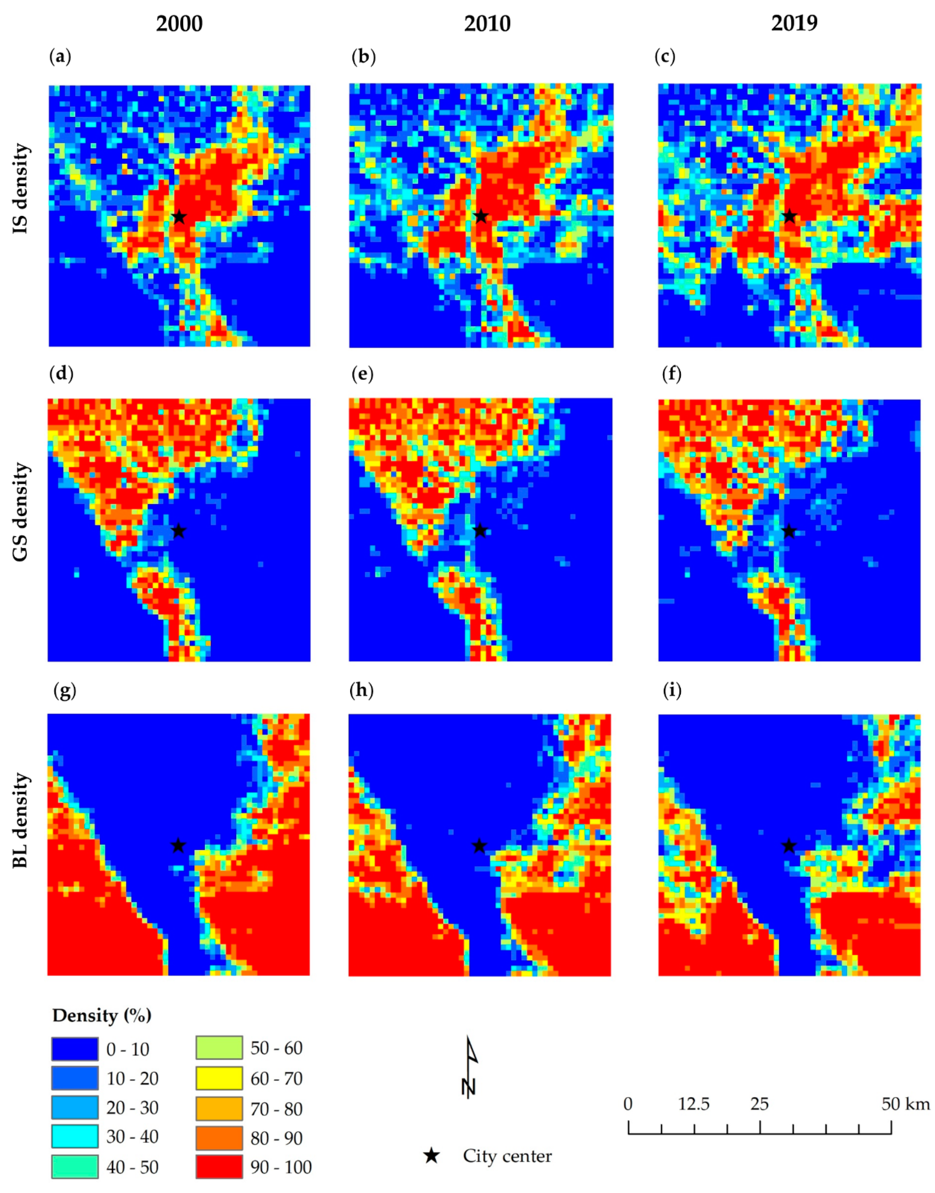
2.4. MODIS LST and Density of IS, GS, and BL

The LUC density is apparent in the cross-sectional analysis of the urban–rural gradient of a typical surface UHI profile. Based on the summer daytime/nighttime mean LST, we created a surface UHI intensity profiling for this study. First, kilometer 0, the city center, was allocated (Figure 1c). Second, raster daytime and nighttime LST maps were created by snapping together polygon grids. These polygon grids were 1 $\times$1 km, the same as in previous studies [16]. The densities of IS, GS, and BL were defined as the percentage of the total area within a 1 $\times$1 km grid, which is equal to the MODIS LST data’s spatial resolution. Finally, the relationship between the mean LST and the urban intensity measured on each grid was examined using bivariate correlation analysis and scatter plot diagrams. We excluded the water category in this stage.

2.5. Trend in the Daytime and Nighttime Surface UHI Intensity

We examined the mean LST difference ($∆$ mean LST) along the urban–rural gradient between the daytime and nighttime. All 1 km polygon grids in the same direction were targets of analysis. Four polygons of the surrounding city center (hereafter referred to as the central grid area = 4 km²) were defined as Urban–Rural Zone 1 (URZ₁) ((Appendix A Figure A1). The 25 buffer areas were delineated as urban–rural zones (URZs), e.g., URZ₁, URZ₂, …, URZ₂₅.

Zones derived the daytime and nighttime mean LST and densities of IS, GS, and BL in each URZ at 1 km intervals. The daytime/nighttime change in mean LST between URZ₁ (the zone with the highest urban intensity each year) and other URZs (i.e., URZ₂, URZ₃, ..., URZ₂₅) were defined by the surface UHI intensity. The same procedure was applied for the three time points.

We focused on the URZ with a high IS density as urban zones and URZs with <15% IS density as rural zones [16,91]. The trend in the daytime and nighttime surface UHI intensity was calculated using Equation (1). All the extracted values were plotted along the urban–rural gradient. Scatter plot diagrams were drawn to delineate statistical relationships.

Surface UHI intensity = URZ₁ − URZ_n

(1)

where URZ₁ is the central grid of the urban–rural gradient and n refers to the number of urban–rural zones (i.e., URZ₂, URZ₃, URZ₄, ……, URZ₂₅).

2.6. Population Density Data

WorldPop is a database for estimating the world’s population [92,93]. It provides various types of the gridded population data sets [94]. Numerous researchers have used this population data [95,96,97,98], including United Nations Development Programme (UNDP), World Health Organization (WHO), The World Bank, and the World Wildlife Fund (WWF) [99]. The large population or high population density (PD) of a city contributes to settlement expansion and vertical development of high-rise residential apartments. Indirectly, the PD has become one of the critical factors of urban heat island formation. In this study, 2000, 2010, and 2019 WorldPop data (at a 30 arc-second approximately 1 $\times$1 km resolution) were used to explore the relationship between mean LST and PD in both the daytime and the nighttime in Greater Cairo using scatter plots diagrams and linear regression. We used a 1 km polygon grid, produced in Section 2.4, to extract raster WorldPop PD values.

2.7. Landscape Configuration Analysis

Based on the landscape configuration analysis, we examined how IS, GS, and BL influenced the variability in the LST in Greater Cairo. The grid size used in Section 2.5 was insufficient for this configuration analysis due to the total patch’s possible effect being allocated to 1 km grids. Moreover, instead of identifying a single patch’s optimum size, we found the best configuration of patches in closer proximity. Considering previous studies [12,54,100] and the reasons mentioned above, we applied a relatively large grid size. We used a 5 $\times$ 5 km fishnet to divide the whole study area into 100 sub-parts. Based on other studies [12,54], 25 sub-parts were selected using a random sampling technique. The selected sub-parts represented 25% of the total population. The LUC map in each study area was clipped with fixed 25 polygon grids for further analysis. We determined three class-level spatial matrices: mean patch area (AREA_MN), largest patch index (LPI), and aggregation index (AI) (

Table 1. Class-level metrics used in this study [102].

Spatial Metrics	Formula	Description	Units
Mean patch area (AREA_MN)	$\mathrm{AREA}\_\mathrm{MN}\left(\mathrm{ha}\right)=\frac{{{\displaystyle \sum }}_{\mathrm{j}=1}^{\mathrm{n}}{\mathrm{x}}_{\mathrm{ij}}}{n_i}$	The spatial pattern and heterogeneity of the area.	ha
Largest Patch Index (LPI)	$\mathrm{LPI}=\frac{{\max (\mathrm{a}}_{\mathrm{ij}})}{\mathrm{A}}\times \left(100\right)$	LPI ability to detect the advantages of the LUC.	0–100
Aggregation Index (AI)	$\mathrm{AI}(\%)=\left(\frac{{\mathrm{g}}_{\mathrm{ii}}}{\max \to {\mathrm{g}}_{\mathrm{ii}}}\right)\times \left(100\right)$	The calculation of class-level aggregation in the area.	percentage

Where ${\mathrm{n}}_{\mathrm{i}}$ = number of patches of land use/cover (LUC) class i; n $=$ number of patches; j = total of the specific patch type; ${\mathrm{x}}_{\mathrm{ij}} =$ patch metrics value of patch $\mathrm{ij}$; A = total area of LUC; ${\mathrm{a}}_{\mathrm{ij}}$ = total pixels of patch area ij; ${\mathrm{g}}_{\mathrm{ii}}$  $=$ number of joins between pixels of class type; and $\max \to {\mathrm{g}}_{\mathrm{ii}} =$ maximum number of joins between pixels of class type.

). These spatial metrics have been widely used in previous UHI studies [12,101]. The 8-cell neighbor rule was applied to calculate the three metrics. To analyze the impact of landscape configuration on LST, the generated metric values were compared with the mean LST of the LUC classes of each sub-part.

3. Results

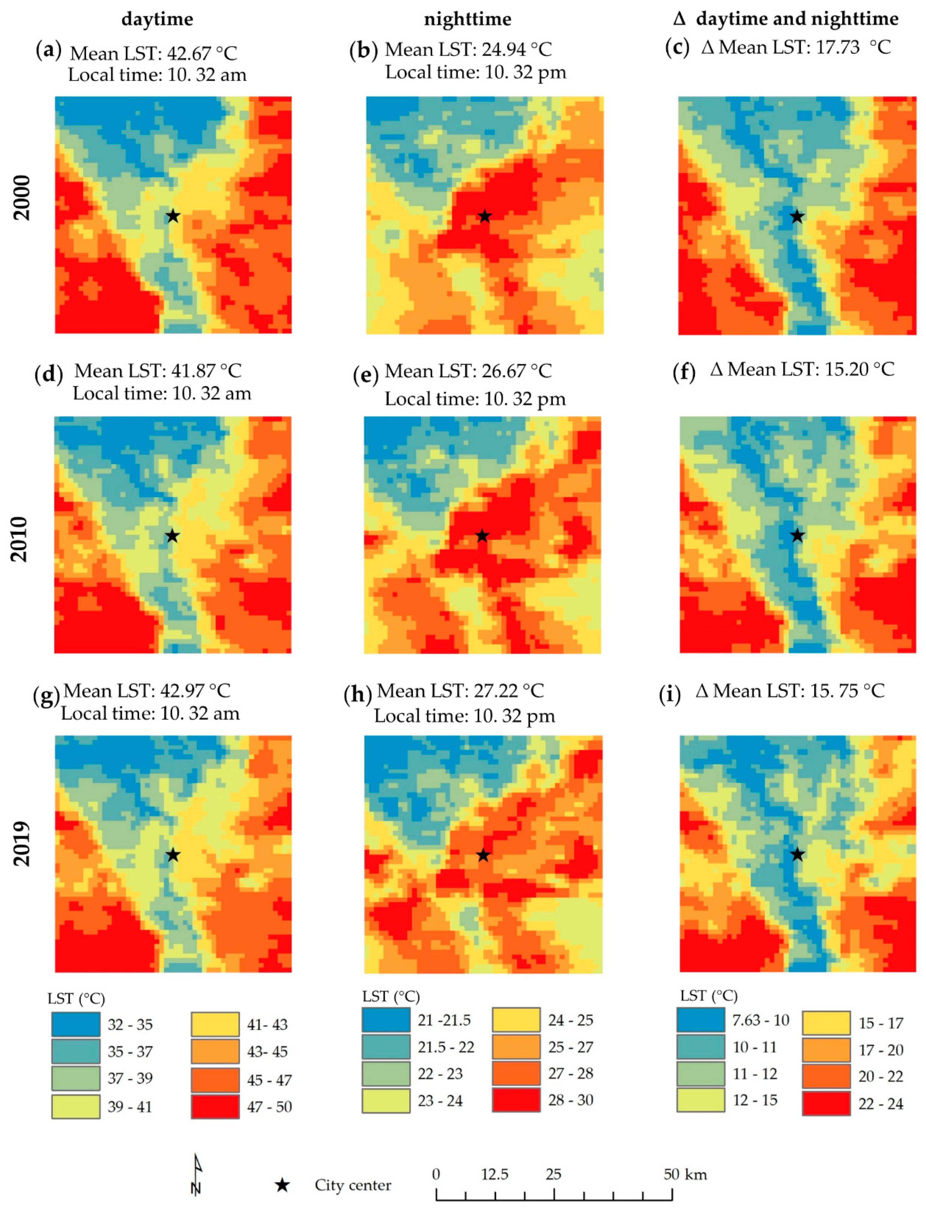
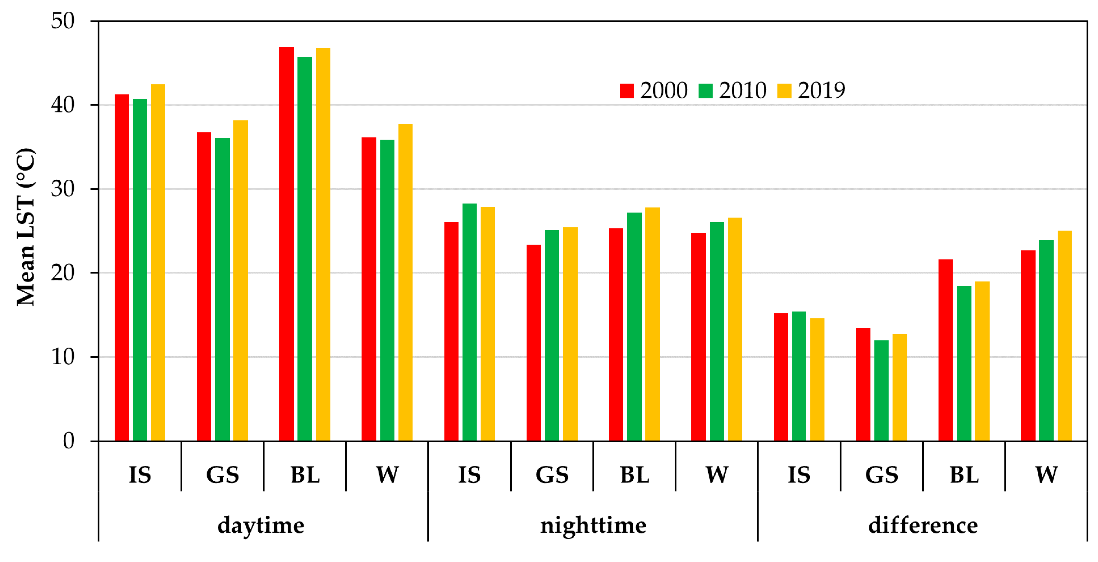
3.1. LUC Changes and Magnitude and Trends of LST

The classified LUC maps in 2000, 2010, and 2019 show that Greater Cairo has undergone rapid urbanization over the 19-year period (Figure 2). From 2000 to 2010, the IS area increased from 564.14 to 698.65 km²; and from 2010 to 2019, the IS area increased by 171 km², with a total gain of 305.21 km² (

Table 2. Area change in the LUC in the study area.

	2000		2010		2019
Land Class	Area (km2)	%	Area (km2)	%	Area (km2)	%
Impervious surface	564.14	22.57	698.65	27.95	869.35	34.77
Greenspace	699.31	27.97	639.52	25.58	627.48	25.1
Bare land	1192.12	47.68	1121.56	44.86	962.93	38.52
Water	44.43	1.78	40.27	1.61	40.24	1.61

). The increase in the IS area in the 2010–2019 period was faster than in the 2000–2009 period. The GS and BL areas showed a decrease, i.e., a total net loss of 71.83 km² and 229.19 km² from 2000 to 2019, respectively. Overall, the IS area has greatly enlarged by rapid urbanization in Greater Cairo.

Figure 3 shows the density of IS, GS, and BL with a 1 $\times$ 1 km grid size. Figure 4 shows the mean LST of Greater Cairo in the daytime/nighttime in 2000, 2010, and 2019. The mean LST in the daytime was 42.67, 41.87, and 42.97 °C in 2000, 2010, and 2019, respectively. The mean LST in the nighttime was 24.94, 26.67, and 27.22 °C in 2000, 2010, and 2019, respectively. The mean LST difference (∆ mean LST) between the daytime and nighttime was 17.73 °C in 2000, 15.20 °C in 2010, and 15.75 °C in 2019 (Figure 4). The ∆ mean LST was small in the central region and large in the surrounding area in the three time points.

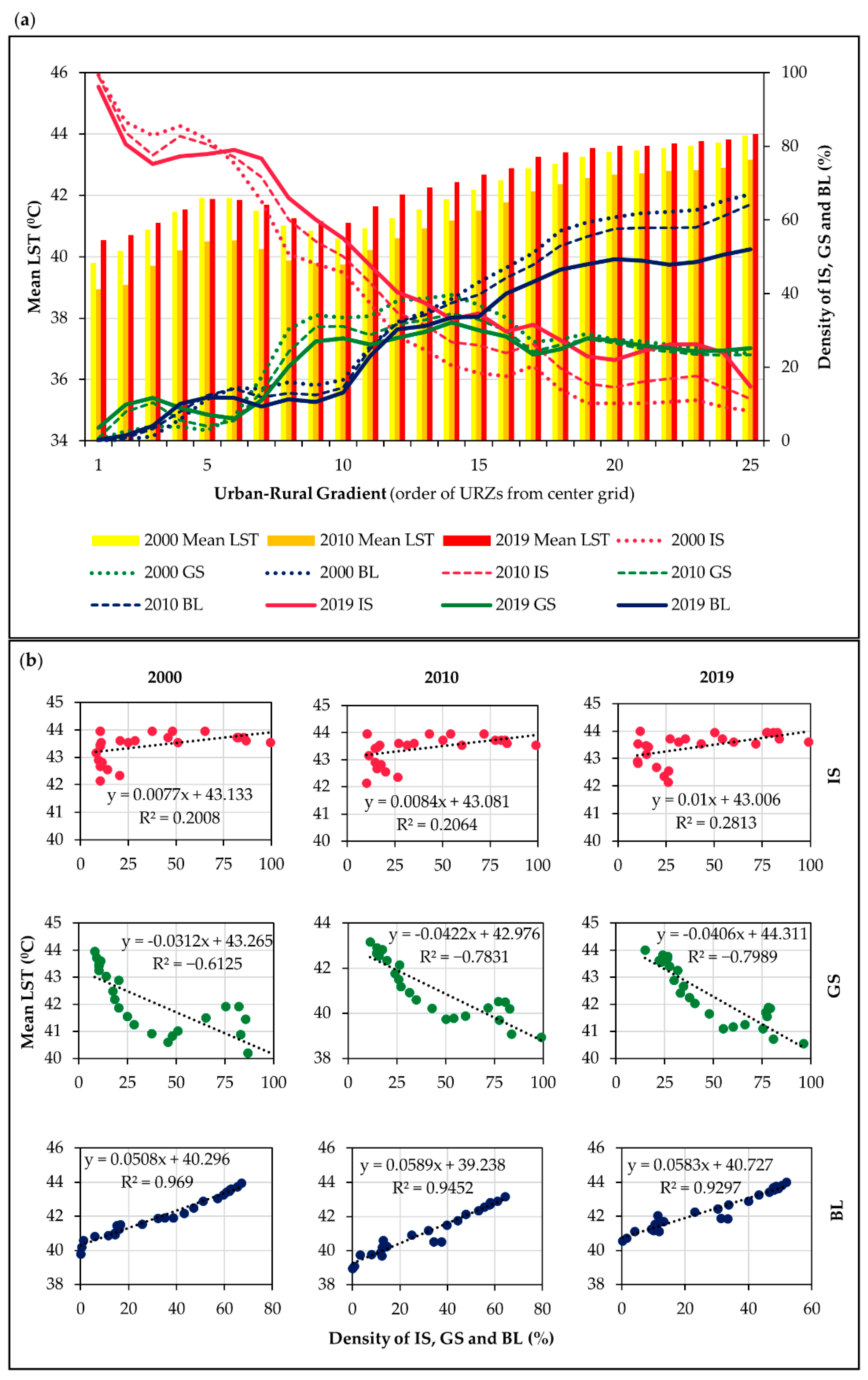
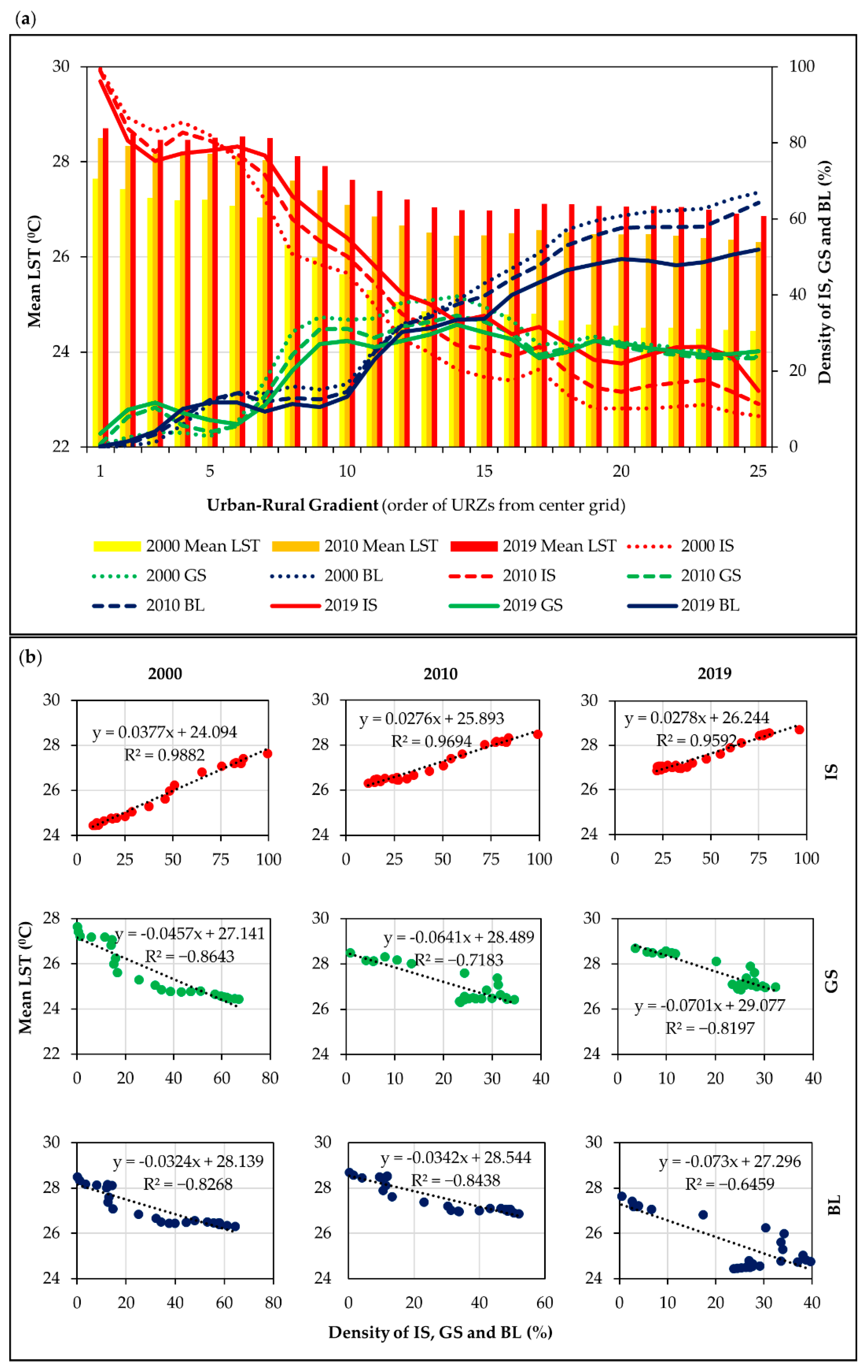
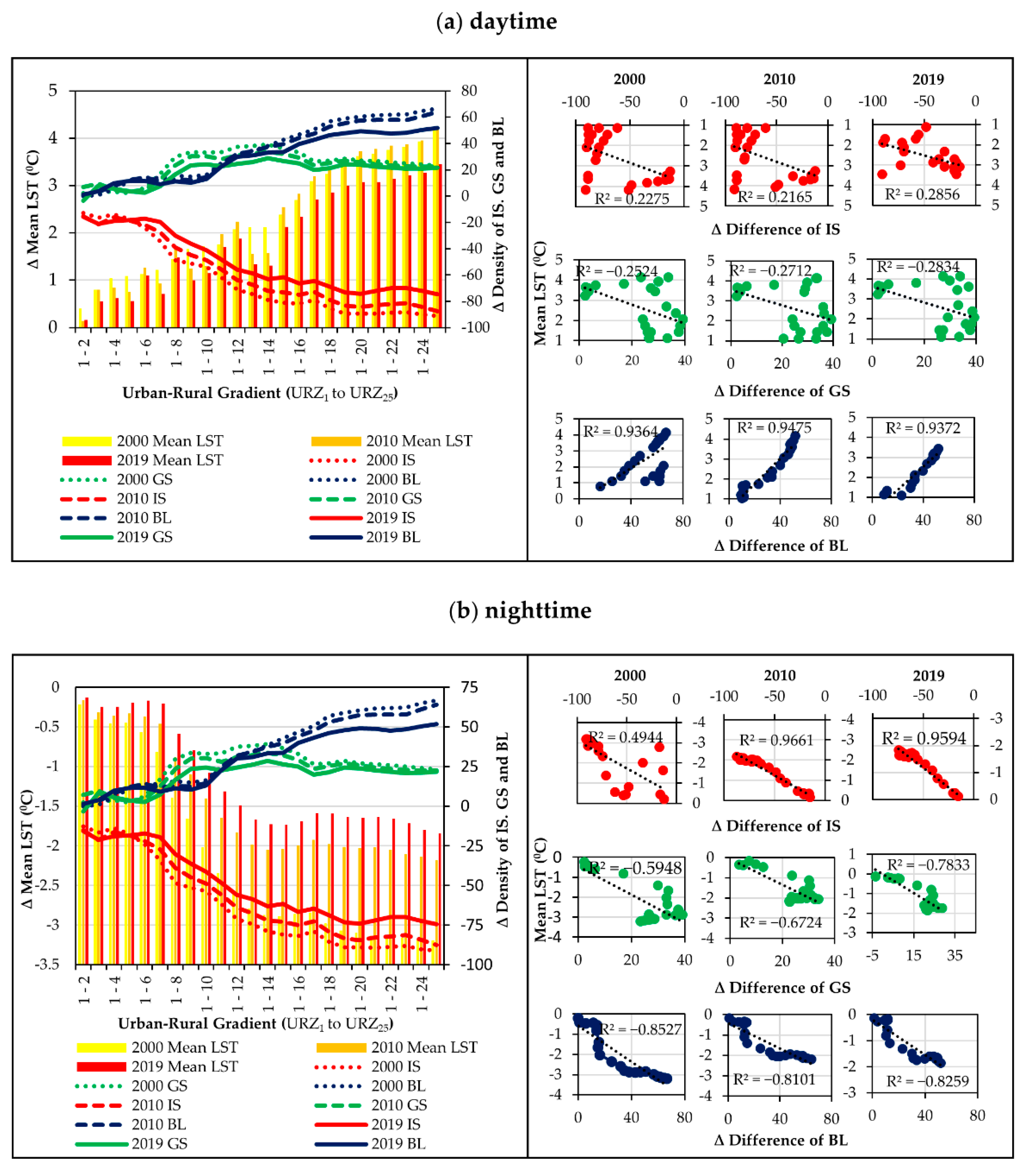
3.2. Mean LST vs. Density of IS, GS, and BL

Figure 5 indicates the derived mean LST of four LUC types: IS, GS, BL, and W (water). In the daytime, BL had the highest mean LST in the three time points. The mean LST difference (daytime—nighttime) of IS was 15.23, 15.63, and 14.59 °C, while that of BL was 21.58, 18.45, 18.99 °C in 2000, 2010, and 2019, respectively. In the nighttime, the mean LST of the four LUC types was lower compared with the daytime mean LST. Though GS showed the lowest mean LST among the four types at the three time points, the difference in the four types was not as large in the nighttime. This means that the impacts of IS and BL on the LST increase were less influential at night.

3.3. Magnitude and Trend of the Surface UHI Intensity in the Daytime and Nighttime

The highest density of IS was in URZ₁ over time (>96.39% in 2000, >97.98% in 2010, and >99.21% in 2019) (urban zone), whereas the boundaries between the urban and rural zones with <15% density of IS were in URZ₁₉ in 2000, URZ₂₃ in 2010, and URZ₂₅ in 2019 (Figure 6 and Figure 7). The urban–rural gradient analysis showed an almost similar trend in the three periods. The composition ratio of the IS in 1–6 km zones decreased, while the composition ratio of the IS in 7–25 km zones increased from 2000 to 2019. In the daytime, the central grid area (URZ₁) had the lowest mean LST (Figure 6a). Then, the mean LST gradually rose with an increase in distance. However, the mean LST tended to drop slowly from 6 to 9 km, and after 10 km, it began to rise again. Along the same line, the IS density and BL density revealed a consistent pattern with mean LST. GS density showed an inverse relationship with mean LST. The statistical analysis based on the 25 URZs indicated positive correlations between the mean LST and the IS density in the daytime. The GS density showed a high negative correlation, and the BL density had a high positive correlation with the mean LST ($\rho$< 0.001) in the daytime (Figure 6b).

Figure 7 shows the urban–rural gradient pattern in the nighttime. In 2000, 2010, and 2019, the mean LST increased gradually between URZ₁ and URZ₇ (i.e., approximately 8 km), and then, the 2000 mean LST decreased rapidly after URZ7, whereas the 2010 and 2019 decreases were more gradual (Figure 7a). After URZ₁₃, the mean LST gradually increased until URZ₂₅ at the three time points. We conclude that the area of surface UHIs in the nighttime enlarged spatially over time. Overall, the correlation analysis indicated a high positive correlation between the mean LST and the density of IS in the nighttime. Conversely, the density of GS and the density of BL had a high negative correlation with the mean LST in the nighttime ($\rho$< 0.001) (Figure 7b). Notably, the correlations of mean LST with IS density in the nighttime were higher than in the daytime in the three periods.

Figure 8 shows the actual situation of surface UHI intensity in the daytime and nighttime in greater Cairo. We use negative values of daytime (based on Equation (1)) as positive values (Figure 8a) and positive values in the nighttime (based on Equation (1)) as negative values (Figure 8b) along the urban–rural gradient because, in the daytime, the urban zones in Greater Cairo (central grid area) experienced an urban cool island effect; in contrast, in the nighttime, urban heat islands were recognized, and the influence became stronger over time. The analysis revealed that the change in mean LST between URZ₁ to URZ₂₅ gradually increased with distance in the daytime, whereas the change in mean LST between them gradually decreased in the nighttime. The difference in daytime surface UHI intensity (between the urban zone and rural zone) was 3.45 °C in 2000, 3.87 °C in 2010, and 3.46 °C in 2019 (Figure 8a). The nighttime surface UHI intensity was –3.07 °C in 2000, −2.10 °C in 2010, and −1.84 °C in 2019 (Figure 8b). In the daytime, we observed a correlation between the change in mean LST and the change in density of IS (positive), the change in density of GS (negative), and the change in density of BL (positive) (Figure 8a). In the nighttime, we observed a strong relationship between the changes in mean LST and density of IS (positive), the change in density of GS (negative), and the change in density of BL (negative) ($\rho$< 0.001; Figure 8b).

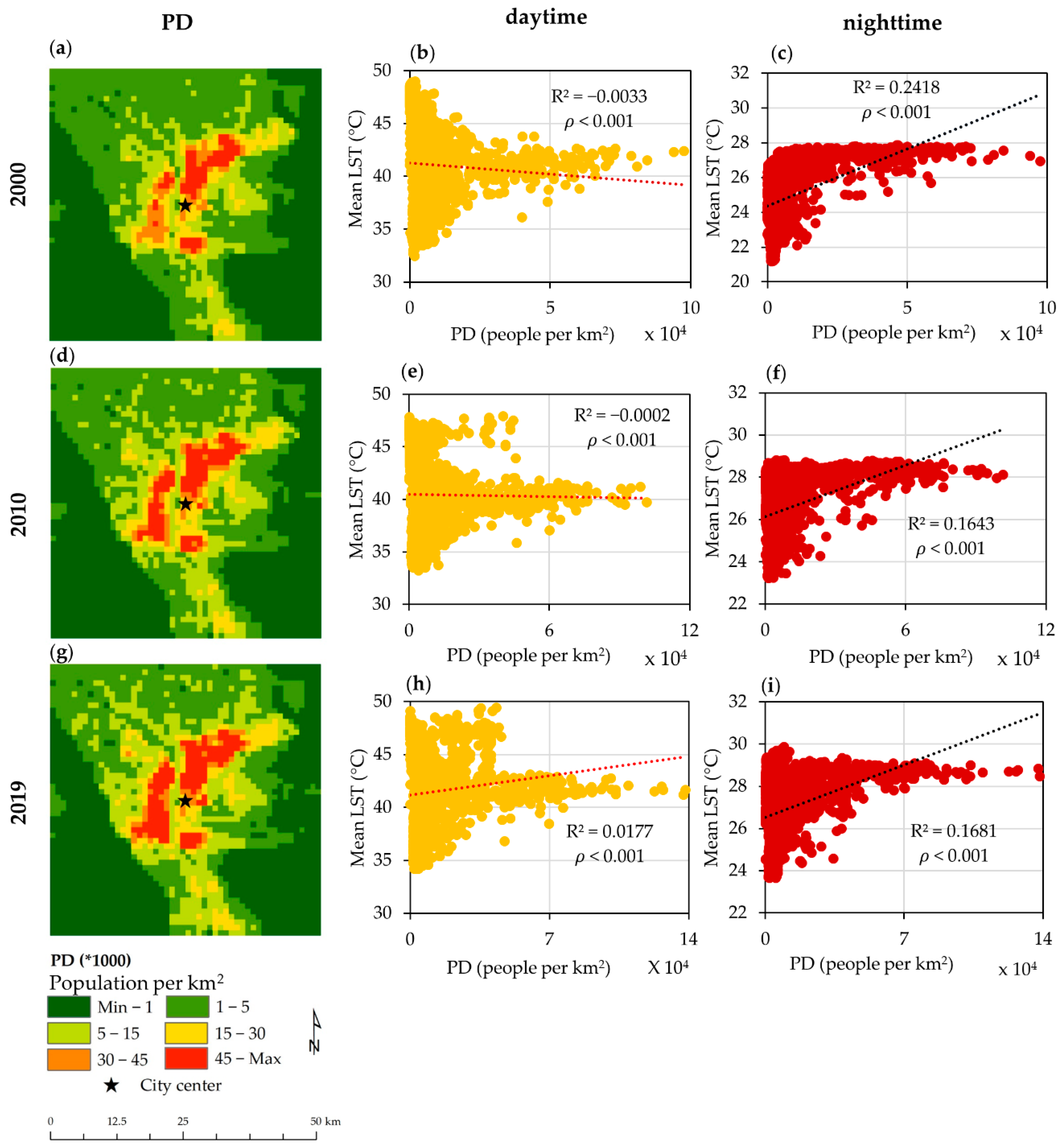
3.4. Population Desnisty vs. LST

Figure 9 shows the PD maps of Greater Cairo in 2000, 2010, and 2019. The PD increased between 2000 and 2019, mainly in the center, east, and north of the study area due to rapid urban expansion and economic development. The results revealed that the population of Greater Cairo was shifting from the city core outward. The relationship between the mean LST and PD was not well-correlated in the daytime (coefficient of determination (R²) = –0.0033 in 2000, R² = –0.0002 in 2010, and R² = 0.0177 in 2019). However, a positive correlation between mean LST and PD was indicated in the nighttime (R² = 0.2418 in 2000, R² = 0.1643 in 2010, and R² = 0.1681 in 2019). All the data analyses were statistically significant ($\rho$< 0.001). We estimated that energy use in the nighttime would cause the warming of the densely habited regions and industries.

3.5. Spatial-Metrics-Based Analysis vs. LST

The LUC types had a possible nexus with LST (

Table 3. Correlation results (r values) between three spatial metrics and mean LST.

Daytime
	2000			2010			2019
	IS	GS	BL	IS	GS	BL	IS	GS	BL
AREA_MN	0.0198	−0.4022	0.3813	0.0169	−0.3621	0.525	0.0200	−0.5001	0.5209
LPI	0.0454	−0.5238	0.6233	0.2001	−0.5123	0.3494	0.0334	−0.5448	0.6054
AI	0.0479	−0.0989	0.6036	0.0202	−0.0897	0.5989	0.004	−0.4047	0.4503
Nighttime
AREA_MN	0.2624	−0.4489	0.0004	0.1745	−0.4007	0.0006	0.199	−0.5873	0.0087
LPI	0.5077	−0.6199	0.0081	0.5700	−0.6038	0.0097	0.4332	−0.6563	0.0318
AI	0.3210	−0.2237	0.1708	0.2536	−0.296	0.1953	0.3584	−0.3781	0.1403

Note: IS = Impervious surface; GS = Green space; BL = Bare land; AREA_MN = Mean Patch Area; LPI = Largest Patch Index; and AI = Aggregation Index.

), and all the results were statistically significant ($p=$0.000). In the daytime, the three indices of AREA_MN, LPI, and AI were positively correlated with the mean LST for BL, but they were not as strongly correlated with IS in the three periods. Conversely, the results showed the opposite condition with IS in the nighttime from 2000 to 2019.

All three indices showed negative relationships with mean LST for GS both in the daytime and nighttime (Table 3). In the daytime, the values of AI of GS indicated more fragmentation in 2000 than in 2010, and it became less fragmented by 2019, which is proof of the negative impact of a strong aggregation with the mean LST. However, GS’s AI results of the nighttime showed less fragmentation of GS from 2000 to 2019 (r = −0.2237 in 2000, r = −0.296 in 2010, and r = −0.3781 in 2019) compared with the daytime.

The increase in LPI values of IS in both the daytime and the nighttime shows that mean patches of IS were less fragmented in 2010 than in 2000, and they became more fragmented by 2019. Our findings also indicated that large IS patches promoted a significant heat effect, whereas smaller IS patches generated a lower surface UHI effect. The LPI results in the daytime showed that the mean patches of BL were more fragmented in 2010 than in 2000. It became less fragmented by 2019, indicating the strong positive impacts of large patches with the mean LST. Conversely, these values indicated a low positive influence in the nighttime.

4. Discussion

4.1. Rapid Urbanization and Its Impact on Greater Cairo

Previous studies showed that rapid urbanization increased informal settlements and environmental degradation in developing countries [103,104]. According to the World Urbanization Prospects Report, Greater Cairo’s population is projected to rise from 5.7 million in 1970 to 14.7 million in 2025 [105]. In 1969, the President of Egypt proposed a master plan for establishing new towns on the fringes of the Cairo desert area [72]. As a result of this project, Greater Cairo has undergone scattered urban expansion. It is estimated that many surrounding desert areas will change to built-up environments in the not-too-distant future, primarily in the eastern side of Greater Cairo. Our results showed that Greater Cairo had experienced rapid urbanization in the 19-year period. Similar results reported by Mohamed and Worku [106] for Addis Ababa and its surrounding environment in Africa (built-up areas increased 3.7% in 2005, 5.7% in 2011, and 7% in 2015, whereas natural environment and agricultural lands were in continuous decline. Siddiqui et al. [107] found that the urban growth rate increased (4.6% in 1993 to 26% in 2013) in Uttar Pradesh of the Indian metropolitan, showing scattered and infilling urban expansion. Han and Jia [108] found that urban areas grew by 590 km² from 1995 to 2015, with a 4% annual growth rate, while agricultural areas declined to 397 km² by 2015 in Foshan, China. The urban development policies for Greater Cairo will enable the use of desert areas for urban sustainability through the advances in industrial zones and the transportation system with balanced control of urban expansion [109].

Greater Cairo’s urbanization has transformed the natural landscape to IS areas, including buildings, roads, and other human-made surface materials, enhancing the surface UHI effect. Surface features such as buildings, roads, and other IS areas can absorb more solar radiation than natural surface areas [12]. Due to daytime solar radiation, these IS areas absorb more solar energy, but the absorbed solar energy is released during the night. As a result, the surface UHI effect over city areas is more pronounced than in the surrounding natural areas during the nighttime because, at night, there is no solar energy. Still, the urban core area of Greater Cairo shows an urban heat island effect (Figure 4 and Figure 8), and the green spaces, which help to reduce urban heat at nighttime, of city area is relatively small compared with the surrounding area (Figure 8). The outcome of the study analysis revealed the significant influence of urbanization on the spatial intensity of the surface UHI effect.

4.2. Surface UHI Nexus with LUC Classes and PD

In Greater Cairo, studying surface UHI in both daytime and nighttime is critical because the city is located in a hot desert region, and a large portion of the area is covered by desert sand (Figure 2). Another important factor is its LUC composition: the northern part of Greater Cairo is covered by green areas (Figure 2). Our findings revealed that the surface UHI gradually increased from the central grid (URZ₁) in the daytime and gradually decreased in the nighttime. There was a significant difference between LUC categories in the daytime (Figure 8). Conversely, there was no substantial difference between them in the nighttime (Figure 5). The surface UHI effect in the nighttime did not fully correspond with LUC categories (Figure 4 and Figure 5), indicating that another mechanism works to produce the nighttime surface UHI effect. Therefore, it is crucial to examine why these phenomena happen in Greater Cairo.

First, the urban cool island effect was prominent in the daytime CBD. The decline in IS density and increase in GS density in the central area promoted the cooling effect in the daytime (Figure 6). Cairo’s government announced a provisioning service in the urban green areas such as green roofs and urban agriculture at the rooftop [110], green corridors, urban parks, green pedestrian, green parking for buses and taxis, as well as urban planning mainly in the urban core area and its environs [111]. These projects have promoted the urban cool island effect in the daytime. Building shading also affects LST more significantly than tree shading because there are more high-rise buildings in the city core area than trees and many buildings have a light roof, producing a positive effect on the energy balance. The suburban area showed high-temperature values in the daytime because IS density gradually increased with distance. New urban development projects have been constructed on desert sand without proper green space planning.

Second, the LUC categories did not substantially promote the surface UHI effect during the nighttime. As mentioned above, due to the daytime solar radiation, such IS areas absorb more solar energy, but in the nighttime, the absorbed solar energy is released. Another factor is anthropogenic activities. Our result revealed a positive correlation between PD and mean LST during the nighttime (Figure 9), indicating that anthropogenic heat released from industry, traffic, and air conditioners from apartments has promoted the surface UHI effect in the nighttime. Light-color paints, urban materials, and cool building materials would help to decrease the temperature. Urban water is also one solution to adopt to mitigate the surface UHI phenomenon in the nighttime [112]. Home gardens should also be promoted during landscape and urban planning to minimize the surface UHI effect during the nighttime.

4.3. Trend in Surface UHI Intensity along the Urban–Rural Gradient

Based on MODIS surface temperature data, the surface UHI effect was identified in the study area (Figure 4). Along with the urban–rural gradient pattern, the lowest LST appeared in the CBD. In contrast, the highest LST appeared 17 to 25 km away from the city center, with a difference in surface UHI intensity between urban zone and rural zone −3.45 °C in 2000, −3.87 °C in 2010, and −3.45 °C in 2019 in the daytime (Figure 6). Unlike previous studies in Africa [54,113], the CBD in Greater Cairo experienced the urban cool island phenomena in the daytime. Conversely, the surrounding rural zones experienced a relative rise in the surface temperature compared with the CBD. Several studies around the world have reported the same phenomenon. For instance, Rasul et al. (2015) [114] examined the daytime urban cool island effect in Erbil, Iraqi Kurdistan, using Landsat 8 data. They reported that the urban cool island intensity in the CBD differed from 3.5 to 4.6 °C in comparison with a 10 km buffer zone around the city. Haashemi et al. (2016) [115] explored the seasonal changes in the urban heat island in the semi-arid city of Tehran, Iran, using MODIS and Landsat 8 data. Their findings indicated that surface urban cool islands remained in the daytime (the maximal urban–rural contrast was −4 Kelvin in March). The maximal nighttime value of the urban–rural difference was 3.9 Kelvin in May. Lazzarini et al. (2015) [71] examined urban climate modification (urban heat island study) in eight hot and semi-arid cities in the world, including Abu Dhabi in the United Arab Emirates; Kuwait City in Kuwait; Riyadh in Saudi Arabia; Doha in Qatar; Las Vegas and Phoenix in the U.S.; Biskra, Algeria; and Bikaner, Rajasthan. They revealed that six cities, Abu Dhabi, Kuwait, Las Vegas, Phoenix, Biskra, and Bikaner, showed the cool UHI effect in the central area during the daytime.

The magnitude of the surface UHI intensity changed considerably with LUC types (Figure 5, Figure 6 and Figure 7). However, we found that the LST values of daytime and nighttime were dependent not only on LUC composition but also on different environmental factors such as significant air masses, dust, humidity, and solar radiation when the MODIS thermal band imageries were taken. In the daytime, the zones 8 to 10 km away from the central grid had the lowest drop in the mean LST because these zones had an abundance of the natural environment (e.g., MAZHAR botanical garden area, a large portion of the Nile River, and the Jazīrat Warrāq al Ḩaḑar area) compared with the surrounding areas. The Nile River and expansive green spaces were the sources of cool air in this zone. It is important to note that the urban cool island effect was dominant in the central grid area in the daytime. According to the density analysis, this area was almost covered with IS (96.39% in 2000, 97.98% in 2010, and 99.21% in 2019) (Figure 6 and Figure 7). This means that the IS′s effect temperature rise was less than that of BL. Furthermore, the central areas consisted of mixed land use of IS and GS with the river environment. The zones stretching from 3 to 7 km did not show a significant cooling island effect along the urban–rural gradient.

In the nighttime, the density of IS was the critical factor in the increase in the urban heat effect in the CBD (Figure 7). Thermal energy absorbed in the daytime is released at nighttime, contributing to the rise in surface UHI [12,116]. In contrast, we observed that the highest mean LST dropped in areas 12 to 16 km away from the city center because green-related land use was dominant in these zones (Figure 7), e.g., cropland and different kinds of desert vegetation such as low canopy trees, shrubs, herbs, and water-based plants (cactus). The daytime and nighttime and urban–rural anomalies were related to the LUC composition. In the nighttime, the impervious surface enhanced surface UHI intensity, combined with the effect of anthropogenic activities.

Though most surface UHI intensity studies have used IS and GS as explanatory variables [56,117,118], a few studies have focused on spatial urban–rural gradient patterns [72]. The variation in the change in mean LST along the urban–rural gradient provides a clue for future urban design and urban thermal mitigation strategies. In our study, the change in surface UHI intensity was examined through surface temperature variations (the change in mean LST) along the urban–rural gradient, i.e., between the density of IS, GS, and BL and between urban–rural zones in the daytime and nighttime at three time points (Figure 8). We compared the results of surface UHI intensities over time. We examined the overall increase and decrease in the surface UHI intensity in the daytime and nighttime in the study area (Figure 8). Along the urban–rural gradient, the rise in surface UHI intensity from 2000 to 2019 based on the urban zone (the highest density of IS) and the rural zone (the lowest density of IS < 15%) was –3.41 °C lower in the daytime and was 2.1 °C higher in the nighttime. Notably, the surface UHI intensity fluctuated (either increasing or decreasing) at critical thresholds along the urban–rural gradient.

To the best of our knowledge, no previous studies identified the critical threshold of surface UHI intensity for LST change along the urban–rural gradient. However, most studies proved that the surface UHI effect is most critical in summer [34]. We determined the threshold value of using URZs to clearly explain the mean LST variations in the urban and rural zones in the daytime and nighttime. The urban design is less aggregated in urban settings, an increase in irregular vegetation areas, coupled with small and medium water areas, would be a practical approach to mitigate the surface UHI effect. There is an urgent need for designing a sustainable urban landscape to avoid the risk of strong surface UHI and heatwaves.

4.4. Landscape Configuration on Surface UHI Formation

The AREA_MN, LPI, and AI indices were significantly correlated with mean LST. AREA_MN, LPI, and AI of IS did not substantially influence the daytime LST variation (Table 3). Conversely, the three above-mentioned metrics of IS showed a considerable positive influence on the nighttime LST variation in Greater Cairo, indicating that urban planners must pay attention to the IS category because it promotes the surface UHI effect in the nighttime. However, except for AI, AREA_MN and LPI of GS did not produce large differences in daytime and nighttime (Table 3).

Our findings are similar to those of other studies. For instance, Zhou et al. (2011) [23] revealed a strong correlation of mean patch size and mean shape index with mean LST for IS (positive) and for GS (negative) at the Gwynns Fall watershed in the USA. Li et al. (2012) [119] reported a negative correlation between mean patch size, mean shape index of patches of GS, and mean LST in Beijing, China. Among the three spatial metrics of IS and GS, mean LST showed significant correlations, positive for IS and negative for GS, in both daytime and nighttime in the study area (Table 3). Large patches of GS provide cooling, thus lowering LST more than smaller patches of GS.

Continuous and larger patches of IS provided a stronger surface UHI effect than smaller patches of IS in both daytime and nighttime. The area experienced a stronger surface UHI effect in the nighttime than the daytime due to continuous and large patches of IS around the central grid area. Human activities in large patches of the IS area have supported the increase in the nighttime temperature due to anthropogenic heat release, the use of nighttime air conditioners, and traffic in the urban core area. Additionally, BL’s continuous and large patches produced a strong surface UHI effect in the daytime in Greater Cairo. In contrast, the same condition was sufficiently influential in producing the cool island effect in the nighttime in Greater Cairo (Figure 4 and Figure 8).

In general, fragmented green areas are less effective in mitigating the surface UHI effect in urban areas. Therefore, we suggest increasing vegetation and ponds in urban areas, introducing green roofs and green walls, and other such practical strategies to mitigate the strong surface UHI effect in desert cities like Greater Cairo.

5. Conclusions

We examined the spatial change in the local climate of Greater Cairo influenced by the surface UHI phenomenon in recent decades. MODIS LST data were used to study the daytime and nighttime temperature distribution using the urban–rural gradient and landscape-metrics-based analysis. The LUC classification showed that Greater Cairo had experienced rapid urbanization since 2000. The AREA_MN, LPI, and AI of the patches of IS (positive) and GS (negative) indicated strong correlations with mean LST at the three time points. The central area (URZ₁) in Greater Cairo has experienced the cool island effect in the daytime but the surface UHI effect in the nighttime. The IS density and mean LST had a week (positive) correlation in the daytime but a strong positive relationship in the nighttime. The surface UHI formation in the nighttime did not correspond with the LUC categories compared with the surface UHI formation in the daytime, indicating anthropogenic activities that strengthen the surface UHI effect.

The urban–rural gradient serves as a unique natural opportunity to identify and mitigate environmental distortion. The urban–rural gradient analysis and landscape-metrics-based analysis are beneficial for predicting the surface UHI surface and its nexus with spatial-temporal LUC changes in future surface UHIs.

We discussed the importance of increasing vegetative cover to reduce IS in Greater Cairo. Urban landscape planners must pay attention to the 1 to 11 km zones where the mean LST is high and GS density is low. It is time to mitigate the surface UHI effect in Greater Cairo by increasing green cover and dispersing the dense building distribution. In this situation, it is vital to introduce green roofs and green walls, grow clustering or irregular trees with large crowns, and construct small- and medium-sized water ponds to cope with the rising surface UHI.

References

1. Reba, M.; Seto, K.C. A systematic review and assessment of algorithms to detect, characterize, and monitor urban land change. Remote Sens. Environ. 2020, 242, 111739. [Google Scholar] [CrossRef]
2. Estoque, R.C.; Murayama, Y. Quantifying landscape pattern and ecosystem service value changes in four rapidly urbanizing hill stations of Southeast Asia. Landsc. Ecol. 2016, 31, 1481–1507. [Google Scholar] [CrossRef]
3. Wu, J. Urban sustainability: An inevitable goal of landscape research. Landsc. Ecol. 2010, 25, 1–4. [Google Scholar] [CrossRef] [Green Version]
4. Zhang, D.; Xu, J.; Zhang, Y.; Wang, J.; He, S.; Zhou, X. Study on sustainable urbanization literature based on Web of Science, scopus, and China national knowledge infrastructure: A scientometric analysis in CiteSpace. J. Clean. Prod. 2020, 264, 121537. [Google Scholar] [CrossRef]
5. IPCC. Climate Change 2014: Synthesis Report; Contribution of Working Groups I, II and III to the Fifth Assessment Report of the Intergovernmental Panel on Climate Change; Core Writing Team, Pachauri, R.K., Meyer, L.A., Eds.; IPCC: Geneva, Switzerland, 2014. [Google Scholar]
6. Qiu, T.; Song, C.; Zhang, Y.; Liu, H.; Vose, J.M. Urbanization and climate change jointly shift land surface phenology in the northern mid-latitude large cities. Remote Sens. Environ. 2020, 236, 111477. [Google Scholar] [CrossRef]
7. Marcotullio, P.J.; Keßler, C.; Fekete, B.M. The future urban heatwave challenge in Africa: Exploratory analysis. Glob. Environ. Chang. 2021, 66. [Google Scholar] [CrossRef]
8. Franco, S.; Mandla, V.R.; Ram Mohan Rao, K. Urbanization, energy consumption and emissions in the Indian context A review. Renew. Sustain. Energy Rev. 2017, 71, 898–907. [Google Scholar] [CrossRef]
9. Michishita, R.; Jiang, Z.; Xu, B. Monitoring two decades of urbanization in the Poyang Lake area, China through spectral unmixing. Remote Sens. Environ. 2012, 117, 3–18. [Google Scholar] [CrossRef]
10. Grimm, N.B.; Faeth, S.H.; Golubiewski, N.E.; Redman, C.L.; Wu, J.; Bai, X.; Briggs, J.M. Global change and the ecology of cities. Science 2008, 319, 756–760. [Google Scholar] [CrossRef] [Green Version]
11. Cao, H.; Chao, S.; Qiao, L.; Jiang, Y.; Zeng, X.; Fan, X. Urbanization-related changes in soil PAHs and potential health risks of emission sources in a township in Southern Jiangsu, China. Sci. Total Environ. 2017, 575, 692–700. [Google Scholar] [CrossRef]
12. Estoque, R.C.; Murayama, Y.; Myint, S.W. Effects of landscape composition and pattern on land surface temperature: An urban heat island study in the megacities of Southeast Asia. Sci. Total Environ. 2017, 577, 349–359. [Google Scholar] [CrossRef] [PubMed]
13. Zhang, X.; Estoque, R.C.; Murayama, Y. An urban heat island study in Nanchang City, China based on land surface temperature and social-ecological variables. Sustain. Cities Soc. 2017, 32, 557–568. [Google Scholar] [CrossRef]
14. Howard, L. The Climate of London, Deduced from Meteorological Observations; Cambridge University Press: New York, NY, USA, 2012; Volume 2. [Google Scholar]
15. OKE, T.R. City size and the urban heat island. Atmos. Environ. 1973, 7, 769–779. [Google Scholar] [CrossRef]
16. Estoque, R.C.; Murayama, Y. Monitoring surface urban heat island formation in a tropical mountain city using Landsat data (1987–2015). ISPRS J. Photogramm. Remote Sens. 2017, 133, 18–29. [Google Scholar] [CrossRef]
17. Wang, Y.; Hu, B.K.H.; Myint, S.W.; Feng, C.; Chow, W.T.L.; Passy, P.F. Science of the Total Environment Patterns of land change and their potential impacts on land surface temperature change in Yangon, Myanmar. Sci. Total Environ. 2018, 643, 738–750. [Google Scholar] [CrossRef] [PubMed]
18. Pereira Filho, A.J.; Karam, H.A. Urban Climate Estimation of long term low resolution surface urban heat island intensities for tropical cities using MODIS remote sensing data. UCLIM 2016, 17, 32–66. [Google Scholar] [CrossRef]
19. He, B.J.; Wang, J.; Liu, H.; Ulpiani, G. Localized synergies between heat waves and urban heat islands: Implications on human thermal comfort and urban heat management. Environ. Res. 2021, 193, 110584. [Google Scholar] [CrossRef] [PubMed]
20. Zhao, L.; Lee, X.; Smith, R.B.; Oleson, K. Strong contributions of local background climate to urban heat islands. Nature 2014, 511, 216–219. [Google Scholar] [CrossRef]
21. Weng, Q.; Fu, P.; Gao, F. Generating daily land surface temperature at Landsat resolution by fusing Landsat and MODIS data. Remote Sens. Environ. 2014, 145, 55–67. [Google Scholar] [CrossRef]
22. Gillies, R.R.; Kustas, W.P.; Humes, K.S. A verification of the “triangle” method for obtaining surface soil water content and energy fluxes from remote measurements of the Normalized Difference Vegetation Index (NDVI) and surface e. Int. J. Remote Sens. 1997, 18, 3145–3166. [Google Scholar] [CrossRef]
23. Zhou, W.; Huang, G.; Cadenasso, M.L. Does spatial configuration matter? Understanding the effects of land cover pattern on land surface temperature in urban landscapes. Landsc. Urban Plan. 2011, 102, 54–63. [Google Scholar] [CrossRef]
24. Wang, Y.; Du, H.; Xu, Y.; Lu, D.; Wang, X.; Guo, Z. Temporal and spatial variation relationship and influence factors on surface urban heat island and ozone pollution in the Yangtze River Delta, China. Sci. Total Environ. 2018, 631–632, 921–933. [Google Scholar] [CrossRef] [PubMed]
25. Wong, L.P.; Alias, H.; Aghamohammadi, N.; Aghazadeh, S.; Nik Sulaiman, N.M. Urban heat island experience, control measures and health impact: A survey among working community in the city of Kuala Lumpur. Sustain. Cities Soc. 2017, 35, 660–668. [Google Scholar] [CrossRef]
26. Rocklöv, J.; Forsberg, B.; Ebi, K.; Bellander, T. Susceptibility to mortality related to temperature and heat and cold wave duration in the population of Stockholm County, Sweden. Glob. Health Action 2014, 7. [Google Scholar] [CrossRef] [PubMed] [Green Version]
27. Yang, J.; Wang, Y.; Xiu, C.; Xiao, X.; Xia, J.; Jin, C. Optimizing local climate zones to mitigate urban heat island effect in human settlements. J. Clean. Prod. 2020, 275, 123767. [Google Scholar] [CrossRef]
28. Guo, A.; Yang, J.; Sun, W.; Xiao, X.; Xia Cecilia, J.; Jin, C.; Li, X. Impact of urban morphology and landscape characteristics on spatiotemporal heterogeneity of land surface temperature. Sustain. Cities Soc. 2020, 63, 102443. [Google Scholar] [CrossRef]
29. Yang, J.; Zhan, Y.; Xiao, X.; Xia, J.C.; Sun, W.; Li, X. Investigating the diversity of land surface temperature characteristics in different scale cities based on local climate zones. Urban Clim. 2020, 34, 100700. [Google Scholar] [CrossRef]
30. Yao, R.; Wang, L.; Huang, X.; Gong, W.; Xia, X. Greening in Rural Areas Increases the Surface Urban Heat Island Intensity. Geophys. Res. Lett. 2019, 46, 2204–2212. [Google Scholar] [CrossRef]
31. Fast, J.D.; Torcolini, J.C.; Redman, R. Pseudovertical temperature profiles and the urban heat island measured by a temperature datalogger network in Phoenix, Arizona. J. Appl. Meteorol. 2005, 44, 3–13. [Google Scholar] [CrossRef]
32. Chow, W.T.L.; Roth, M. Temporal dynamics of the urban heat island of Singapore. Int. J. Climatol. 2006, 2260, 2243–2260. [Google Scholar] [CrossRef]
33. Yao, R.; Wang, L.; Huang, X.; Chen, J.; Li, J.; Niu, Z. Less sensitive of urban surface to climate variability than rural in Northern China. Sci. Total Environ. 2018, 628–629, 650–660. [Google Scholar] [CrossRef]
34. Zhou, D.; Bonafoni, S.; Zhang, L.; Wang, R. Remote sensing of the urban heat island effect in a highly populated urban agglomeration area in East China. Sci. Total Environ. 2018, 628–629, 415–429. [Google Scholar] [CrossRef]
35. Yao, R.; Wang, L.; Huang, X.; Niu, Z.; Liu, F.; Wang, Q. Temporal trends of surface urban heat islands and associated determinants in major Chinese cities. Sci. Total Environ. 2017, 609, 742–754. [Google Scholar] [CrossRef] [PubMed]
36. Imhoff, M.L.; Zhang, P.; Wolfe, R.E.; Bounoua, L. Remote sensing of the urban heat island effect across biomes in the continental USA. Remote Sens. Environ. 2010, 114, 504–513. [Google Scholar] [CrossRef] [Green Version]
37. Huang, F.; Zhan, W.; Wang, Z.H.; Voogt, J.; Hu, L.; Quan, J.; Liu, C.; Zhang, N.; Lai, J. Satellite identification of atmospheric-surface-subsurface urban heat islands under clear sky. Remote Sens. Environ. 2020, 250, 112039. [Google Scholar] [CrossRef]
38. Li, H.; Zhou, Y.; Li, X.; Meng, L.; Wang, X.; Wu, S.; Sodoudi, S. A new method to quantify surface urban heat island intensity. Sci. Total Environ. 2018, 624, 262–272. [Google Scholar] [CrossRef] [PubMed]
39. Zhou, W.; Wang, J.; Cadenasso, M.L. Effects of the spatial configuration of trees on urban heat mitigation: A comparative study. Remote Sens. Environ. 2017, 195, 1–12. [Google Scholar] [CrossRef]
40. Peng, J.; Xie, P.; Liu, Y.; Ma, J. Urban thermal environment dynamics and associated landscape pattern factors: A case study in the Beijing metropolitan region. Remote Sens. Environ. 2016, 173, 145–155. [Google Scholar] [CrossRef]
41. Kong, F.; Yin, H.; James, P.; Hutyra, L.R.; He, H.S. Effects of spatial pattern of greenspace on urban cooling in a large metropolitan area of eastern China. Landsc. Urban Plan. 2014, 128, 35–47. [Google Scholar] [CrossRef]
42. Zhou, D.; Zhang, L.; Li, D.; Huang, D.; Zhu, C. Climate—Vegetation control on the diurnal and seasonal variations of surface urban heat islands in China. Environ. Res. Lett. 2016, 11, 074009. [Google Scholar] [CrossRef]
43. Zhou, D.; Li, D.; Sun, G.; Zhang, L.; Liu, Y.; Hao, L. Contrasting effects of urbanization and agriculture on surface temperature in eastern China. J. Geophys. Res. Atmos. 2016, 9597–9606. [Google Scholar] [CrossRef] [Green Version]
44. Li, X.; Zhou, Y.; Asrar, G.R.; Imhoff, M.; Li, X. The surface urban heat island response to urban expansion: A panel analysis for the conterminous United States. Sci. Total Environ. 2017, 605–606, 426–435. [Google Scholar] [CrossRef] [PubMed]
45. Santamouris, M. Analyzing the heat island magnitude and characteristics in one hundred Asian and Australian cities and regions. Sci. Total Environ. 2015, 512–513, 582–598. [Google Scholar] [CrossRef]
46. Peng, S.; Piao, S.; Ciais, P.; Friedlingstein, P.; Ottle, C. Surface Urban Heat Island Across 419 Global Big Cities. Environ. Sci. Technol. 2012. [Google Scholar] [CrossRef]
47. Clinton, N.; Gong, P. MODIS detected surface urban heat islands and sinks: Global locations and controls. Remote Sens. Environ. 2013, 134, 294–304. [Google Scholar] [CrossRef]
48. Scott Krayenhoff, E.; Voogt, J.A. Daytime thermal anisotropy of urban neighbourhoods: Morphological causation. Remote Sens. 2016, 8, 108. [Google Scholar] [CrossRef] [Green Version]
49. Stewart, I.D.; Oke, T.R. Local climate zones for urban temperature studies. Bull. Am. Meteorol. Soc. 2012, 93, 1879–1900. [Google Scholar] [CrossRef]
50. Yang, J.; Ren, J.; Sun, D.; Xiao, X.; Xia, J.C.; Jin, C.; Li, X. Understanding land surface temperature impact factors based on local climate zones. Sustain. Cities Soc. 2021, 69, 102818. [Google Scholar] [CrossRef]
51. Alexander, P.J.; Mills, G. Local climate classification and Dublin’s urban heat island. Atmosphere 2014, 5, 755–774. [Google Scholar] [CrossRef] [Green Version]
52. Yang, J.; Luo, X.; Jin, C.; Xiao, X.; Cecilia, J. Spatiotemporal patterns of vegetation phenology along the urban—Rural gradient in Coastal Dalian, China. Urban For. Urban Green. 2020, 54, 126784. [Google Scholar] [CrossRef]
53. Fu, P.; Weng, Q. Variability in annual temperature cycle in the urban areas of the United States as revealed by MODIS imagery. ISPRS J. Photogramm. Remote Sens. 2018, 146, 65–73. [Google Scholar] [CrossRef]
54. Athukorala, D.; Murayama, Y. Spatial Variation of Land Use/Cover Composition and Impact on Surface Urban Heat Island in a Tropical Sub-Saharan City of Accra, Ghana. Sustainability 2020, 12, 7953. [Google Scholar] [CrossRef]
55. Weng, Q.; Liu, H.; Lu, D. Assessing the effects of land use and land cover patterns on thermal conditions using landscape metrics in city of Indianapolis, United States. Urban Ecosyst. 2007, 10, 203–219. [Google Scholar] [CrossRef]
56. Myint, S.W.; Wentz, E.A.; Brazel, A.J.; Quattrochi, D.A. The impact of distinct anthropogenic and vegetation features on urban warming. Landsc. Ecol. 2013, 28, 959–978. [Google Scholar] [CrossRef] [Green Version]
57. Voogt, J.A.; Oke, T.R. Thermal remote sensing of urban climates. Remote Sens. Environ. 2003, 86, 370–384. [Google Scholar] [CrossRef]
58. Lu, L.; Weng, Q.; Guo, H.; Li, Q.; Hui, W. Spatiotemporal Variation of Surface Urban Heat Islands in Relation to Land Cover Composition and Configuration: A Multi-Scale Case Study of Xi’an, China. Remote Sens. 2020, 12, 2713. [Google Scholar] [CrossRef]
59. Osborne, P.E.; Alvares-Sanches, T. Quantifying how landscape composition and configuration affect urban land surface temperatures using machine learning and neutral landscapes. Comput. Environ. Urban Syst. 2019, 76, 80–90. [Google Scholar] [CrossRef]
60. Connors, J.P.; Galletti, C.S.; Chow, W.T.L. Landscape configuration and urban heat island effects: Assessing the relationship between landscape characteristics and land surface temperature in Phoenix, Arizona. Landsc. Ecol. 2013, 28, 271–283. [Google Scholar] [CrossRef]
61. Terfa, B.K.; Chen, N.; Zhang, X.; Niyogi, D. Spatial configuration and extent explains the urban heat mitigation potential due to green spaces: Analysis over Addis Ababa, Ethiopia. Remote Sens. 2020, 12, 2876. [Google Scholar] [CrossRef]
62. Nega, W.; Hailu, B.T.; Fetene, A. An assessment of the vegetation cover change impact on rainfall and land surface temperature using remote sensing in a subtropical climate, Ethiopia. Remote Sens. Appl. Soc. Environ. 2019, 16, 100266. [Google Scholar] [CrossRef]
63. Kabano, P.; Lindley, S.; Harris, A. Evidence of urban heat island impacts on the vegetation growing season length in a tropical city. Landsc. Urban Plan. 2021, 206, 103989. [Google Scholar] [CrossRef]
64. Me-ead, C.; McNeil, R. Pattern and Trend of Night Land Surface Temperature in Africa. Sci. Rep. 2019, 9, 1–8. [Google Scholar] [CrossRef] [PubMed]
65. Effat, H.A.; Hassan, O.A.K. Change detection of urban heat islands and some related parameters using multi-temporal Landsat images; a case study for Cairo city, Egypt. Urban Clim. 2014, 10, 171–188. [Google Scholar] [CrossRef]
66. El-Hattab, M.; Amany, S.M.; Lamia, G.E. Monitoring and assessment of urban heat islands over the Southern region of Cairo Governorate, Egypt. Egypt. J. Remote Sens. Sp. Sci. 2018, 21, 311–323. [Google Scholar] [CrossRef]
67. United Nations Human Settlements Programme. The State of African Cities. 2008. A Framework for Addressing Urban Challenges in Africa; UN-HABITAT: Nairobi, Kenya, 2008; ISBN 9789211320152. [Google Scholar]
68. Kondo, K.; Mabon, L.; Bi, Y.; Chen, Y.; Hayabuchi, Y. Balancing conflicting mitigation and adaptation behaviours of urban residents under climate change and the urban heat island effect. Sustain. Cities Soc. 2021, 65, 102585. [Google Scholar] [CrossRef] [PubMed]
69. Monteiro, F.F.; Gonçalves, W.A.; Andrade, L.D.M.B.; Villavicencio, L.M.M.; dos Santos Silva, C.M. Assessment of Urban Heat Islands in Brazil based on MODIS remote sensing data. Urban Clim. 2021, 35. [Google Scholar] [CrossRef]
70. Richard, Y.; Pohl, B.; Rega, M.; Pergaud, J.; Thevenin, T.; Emery, J.; Dudek, J.; Vairet, T.; Zito, S.; Chateau-Smith, C. Is Urban Heat Island intensity higher during hot spells and heat waves (Dijon, France, 2014–2019)? Urban Clim. 2021, 35, 100747. [Google Scholar] [CrossRef]
71. Lazzarini, M.; Molini, A.; Marpu, P.R.; Ouarda, T.B.M.J.; Ghedira, H. Urban climate modifications in hot desert cities: The role of land cover, local climate, and seasonality. Geophys. Res. Lett. 2015, 42, 9980–9989. [Google Scholar] [CrossRef] [Green Version]
72. Shahraiyni, H.T.; Sodoudi, S.; El-zafarany, A.; Abou, T.; Seoud, E. A Comprehensive Statistical Study on Daytime Surface Urban Heat Island during Summer in Urban Areas, Case Study: Cairo and Its New Towns. Remote Sens. 2016, 8, 643. [Google Scholar] [CrossRef] [Green Version]
73. Robaa, S.M. Some aspects of the urban climates of Greater Cairo Region, Egypt. Int. J. Climatol. 2013, 3216, 3206–3216. [Google Scholar] [CrossRef]
74. The World’s Cities in 2018. Available online: https://www.un.org/development/desa/pd/search/node/the%20world%20cities%20in%202018 (accessed on 4 April 2021).
75. Yin, Z.Y.; Stewart, D.J.; Bullard, S.; MacLachlan, J.T. Changes in urban built-up surface and population distribution patterns during 1986-1999: A case study of Cairo, Egypt. Comput. Environ. Urban Syst. 2005, 29, 595–616. [Google Scholar] [CrossRef]
76. Nile Basin Climate Zones—Nile Basin Water Resources Atlas. Available online: https://atlas.nilebasin.org/treatise/nile-basin-climate-zones/ (accessed on 23 February 2021).
77. Maps and Educational Software. Available online: http://www.yourchildlearns.com/ (accessed on 11 August 2020).
78. DIVA-GIS. Available online: https://www.diva-gis.org/ (accessed on 11 August 2020).
79. Google Earth Engine. Available online: https://earthengine.google.com/ (accessed on 11 August 2020).
80. R: The R Project for Statistical Computing. Available online: https://www.r-project.org/ (accessed on 12 August 2020).
81. Kamusoko, C.; Aniya, M. Hybrid classification of Landsat data and GIS for land use/cover change analysis of the Bindura district, Zimbabwe. Int. J. Remote Sens. 2009, 30, 97–115. [Google Scholar] [CrossRef]
82. Erkan, U.; Gökrem, L. A new method based on pixel density in salt and pepper noise removal. Turk. J. Electr. Eng. Comput. Sci. 2018, 26, 162–171. [Google Scholar] [CrossRef]
83. Thapa, R.B.; Murayama, Y. Image classification techniques in mapping urban landscape: A case study of Tsukuba city using AVNIR-2 sensor data. Tsukuba Geoenviron. Sci. 2007, 3, 3–10. [Google Scholar]
84. Schwarz, N.; Lautenbach, S.; Seppelt, R. Exploring indicators for quantifying surface urban heat islands of European cities with MODIS land surface temperatures. Remote Sens. Environ. 2011, 115, 3175–3186. [Google Scholar] [CrossRef]
85. Wang, K.; Li, Z.; Cribb, M. Estimation of evaporative fraction from a combination of day and night land surface temperatures and NDVI: A new method to determine the Priestley-Taylor parameter. Remote Sens. Environ. 2006, 102, 293–305. [Google Scholar] [CrossRef]
86. Jin, M.; Dickinson, R.E. Land surface skin temperature climatology: Benefitting from the strengths of satellite observations. Environ. Res. Lett. 2010, 5. [Google Scholar] [CrossRef] [Green Version]
87. LP DAAC—MODIS Overview. Available online: https://lpdaac.usgs.gov/data/get-started-data/collection-overview/missions/modis-overview/ (accessed on 10 February 2021).
88. MOD11A1.006 Terra Land Surface Temperature and Emissivity Daily Global 1 km. Available online: https://developers.google.com/earth-engine/datasets/catalog/MODIS_006_MOD11A1 (accessed on 12 August 2020).
89. Image Collection Reductions. Available online: https://developers.google.com/earth-engine/reducers_image_collection (accessed on 12 August 2020).
90. LP DAAC Data User Resources/ArcGIS MODIS Python Toolbox. Available online: https://git.earthdata.nasa.gov/projects/LPDUR/repos/arcgis-modis-python-toolbox/browse (accessed on 10 February 2021).
91. van Hove, L.W.A.; Steeneveld, G.J.; Jacobs, C.M.J.; Heusinkveld, B.G.; Elbers, J.A.; Moors, E.J.; Holtslag, A.A.M. Exploring the Urban Heat Island Intensity of Dutch Cities: Assessment Based on a Literature Review, Recent Meteorologic; Alterra: Wageningen, The Netherlands, 2011. [Google Scholar]
92. Tatem, A.J. WorldPop, open data for spatial demography. Sci. Data 2017, 4, 2–5. [Google Scholar] [CrossRef] [PubMed]
93. Lloyd, C.T. High resolution global gridded data for use in population studies. Int. Arch. Photogramm. Remote Sens. Spat. Inf. Sci. ISPRS Arch. 2017, 42, 117–120. [Google Scholar] [CrossRef] [Green Version]
94. WorldPop. Available online: https://www.worldpop.org/ (accessed on 17 February 2021).
95. Taubenböck, H.; Weigand, M.; Esch, T.; Staab, J.; Wurm, M.; Mast, J.; Dech, S. A new ranking of the world’s largest cities—Do administrative units obscure morphological realities? Remote Sens. Environ. 2019, 232, 111353. [Google Scholar] [CrossRef]
96. Ye, T.; Zhao, N.; Yang, X.; Ouyang, Z.; Liu, X.; Chen, Q.; Hu, K.; Yue, W.; Qi, J.; Li, Z.; et al. Improved population mapping for China using remotely sensed and points-of-interest data within a random forests model. Sci. Total Environ. 2019, 658, 936–946. [Google Scholar] [CrossRef]
97. Estoque, R.C.; Ooba, M.; Seposo, X.T.; Togawa, T.; Hijioka, Y.; Nakamura, S. Heat health risk assessment in Philippine cities using remotely sensed data and social-ecological indicators. Nat. Commun. 2020, 11, 1–12. [Google Scholar] [CrossRef] [PubMed] [Green Version]
98. Zhao, X.; Liu, J.; Bu, Y. Quantitative Analysis of Spatial Heterogeneity and Driving Forces of the Thermal Environment in Urban Built-up Areas: A Case Study in Xi’ an, China. Sustainability 2021, 13, 1870. [Google Scholar] [CrossRef]
99. WorldPop: About WorldPop. Available online: https://www.worldpop.org/about (accessed on 17 February 2021).
100. Hou, H.; Estoque, R.C. Detecting Cooling Effect of Landscape from Composition and Configuration: An Urban Heat Island Study on Hangzhou. Urban For. Urban Green. 2020, 53, 126719. [Google Scholar] [CrossRef]
101. Li, X.; Kamarianakis, Y.; Ouyang, Y.; Turner, B.L.; Brazel, A. On the association between land system architecture and land surface temperatures: Evidence from a Desert Metropolis—Phoenix, Arizona, U.S.A. Landsc. Urban Plan. 2017, 163, 107–120. [Google Scholar] [CrossRef] [Green Version]
102. McGarigal, K. Fragstats; US Department of Agriculture, Forest Service, Pacific Northwest Research Station: Corvallis, OR, USA, 2015; pp. 1–182. [CrossRef]
103. Rady, O.; El-kawy, A.; Ahmed, H.; Mohamed, H. The Egyptian Journal of Remote Sensing and Space Sciences Temporal detection and prediction of agricultural land consumption by urbanization using remote sensing. Egypt. J. Remote Sens. Sp. Sci. 2019, 22, 237–246. [Google Scholar] [CrossRef]
104. Athukorala, D.; Estoque, R.C.; Murayama, Y.; Matsushita, B. Impacts of urbanization on the Muthurajawela marsh and Negombo lagoon, Sri Lanka: Implications for landscape planning towards a sustainable urban wetland ecosystem. Remote Sens. 2021, 13, 316. [Google Scholar] [CrossRef]
105. World Urbanization Prospects, The 2011 Revision; Department of Economic and Social Affairs, Popolation Division, United Nations: New York, NY, USA, 2012.
106. Mohamed, A.; Worku, H. Simulating urban land use and cover dynamics using cellular automata and Markov chain approach in Addis Ababa and the surrounding. Urban Clim. 2020, 31, 100545. [Google Scholar] [CrossRef]
107. Siddiqui, A.; Siddiqui, A.; Maithani, S.; Jha, A.K.; Kumar, P.; Srivastav, S.K. Urban growth dynamics of an Indian metropolitan using CA Markov and Logistic Regression. Egypt. J. Remote Sens. Sp. Sci. 2018, 21, 229–236. [Google Scholar] [CrossRef]
108. Han, Y.; Jia, H. Simulating the spatial dynamics of urban growth with an integrated modeling approach: A case study of Foshan, China. Ecol. Modell. 2017, 353, 107–116. [Google Scholar] [CrossRef]
109. The Strategic Urban Development Master Plan Study for a Sustainable Development of the Greater Cairo Region in the Arab Republic of Egypt; Final Report; General Organization for Physical Planning, Greater Cairo Region Urban Planning Center: Cairo, Egypt; Volume 2, pp. 1–46.
110. Climate Change Adaptation And Urban Resilience Participatory Development Programme in Urban Areas. Available online: http://www.egypt-urban.net/climate-change-adaptation-and-urban-resilience/ (accessed on 22 February 2021).
111. Strategic Urban Development Plan for Greater Cairo Region. UN-HABITAT. Available online: https://mirror.unhabitat.org/content.asp?cid=7120&catid=192&typeid=13 (accessed on 4 April 2021).
112. Rehan, R.M. Cool city as a sustainable example of heat island management case study of the coolest city in the world. HBRC J. 2016, 12, 191–204. [Google Scholar] [CrossRef] [Green Version]
113. Town, B.; Tarawally, M.; Xu, W.; Hou, W.; Mushore, T.D. Comparative Analysis of Responses of Land Surface Temperature to Long-Term Land Use/Cover Changes between a Coastal and Inland City: A Case of Freetown and Bo Town in Sierra Leone. Remote Sens. 2018, 10, 112. [Google Scholar] [CrossRef] [Green Version]
114. Rasul, A.; Balzter, H.; Smith, C. Spatial variation of the daytime Surface Urban Cool Island during the dry season in Erbil, Iraqi Kurdistan, from Landsat 8. Urban Clim. 2015, 14, 176–186. [Google Scholar] [CrossRef] [Green Version]
115. Haashemi, S.; Weng, Q.; Darvishi, A.; Alavipanah, S.K. Seasonal variations of the surface urban heat Island in a semi-arid city. Remote Sens. 2016, 8, 352. [Google Scholar] [CrossRef] [Green Version]
116. USA Environmental Protection Agency Reducing Urban Heat Islands: Green Roofs. Heat Isl. Reduct. Act. 2008, 1–23. [CrossRef]
117. Xu, H.; Lin, D.; Tang, F. The impact of impervious surface development on land surface temperature in a subtropical city: Xiamen, China. Int. J. Climatol. 2013, 1883, 1873–1883. [Google Scholar] [CrossRef]
118. Weng, Q.; Lu, D.; Schubring, J. Estimation of land surface temperature-vegetation abundance relationship for urban heat island studies. Remote Sens. Environ. 2004, 89, 467–483. [Google Scholar] [CrossRef]
119. Li, X.; Zhou, W.; Ouyang, Z.; Xu, W.; Zheng, H. Spatial pattern of greenspace affects land surface temperature: Evidence from the heavily urbanized Beijing metropolitan area, China. Landsc. Ecol. 2012, 27, 887–898. [Google Scholar] [CrossRef]
Figure 2. LUC patterns of Greater Cairo derived from Landsat imagery from GEE (from 2000 to 2019) and K-nearest neighbor classification by R software: (a) LUC map in 2000; (b) LUC map in 2010; and (c) LUC map in 2019.
Remotesensing 13 01396 g002
Figure 3. Distribution of impervious surface (IS), green space (GS), and bare land (BL) densities (1 × 1 km grid) of the study area: (a) IS density in 2000; (b) IS density in 2010; (c) IS density in 2019; (d) GS density in 2000; (e) GS density in 2010; (f) GS density in 2019; (g) BL density in 2000; (h) BL density in 2010; and (i) BL density in 2019.
Remotesensing 13 01396 g003
Figure 4. Land surface temperature (LST) maps of Greater Cairo and its environs derived from Moderate Resolution Imaging Spectroradiometer (MODIS) LST data (2000, 2010, and 2019); (a) daytime mean LST in 2000; (b) nighttime mean LST in 2000; (c) daytime and nighttime mean LST difference in 2000; (d) daytime mean LST in 2010; (e) nighttime mean LST in 2010; (f) daytime and nighttime mean LST difference in 2010; (g) daytime mean LST in 2019; (h) nighttime mean LST in 2019; and (i) daytime and nighttime mean LST difference in 2019. The temperatures are the mean clear-sky LST values observed during July and August.
Remotesensing 13 01396 g004
Figure 5. Mean LST of the LUC types in Greater Cairo, Egypt, in 2000, 2010, and 2019. Note: IS = Impervious surface; GS = Greenspace; BL = Bare land; and W = Water.
Remotesensing 13 01396 g005
Figure 6. Urban–rural gradient analysis in the daytime: (a) mean LST and density of IS, GS, and BL along the urban–rural gradient; and (b) statistical relationships between mean LST and density of IS, GS, and BL.
Remotesensing 13 01396 g006
Figure 7. Urban–rural gradient analysis in the nighttime: (a) mean LST and density of IS, GS, and BL along the urban–rural gradient, and (b) statistical relationships between mean LST and density IS, GS and BL.
Remotesensing 13 01396 g007
Figure 8. The magnitude and trend of surface urban heat island (UHI) intensity (2000–2019): (a) daytime surface UHI intensity and statistical relationships and (b) nighttime surface UHI intensity and statistical relationships.
Remotesensing 13 01396 g008
Figure 9. Population density (PD) of Greater Cairo and its environs: (a) PD in 2000; (b) daytime relationship between mean LST and PD in 2000; (c) nighttime relationship between mean LST and PD in 2000; (d) PD in 2010; (e) daytime relationship between mean LST and PD in 2010; (f) nighttime relationship between mean LST and PD in 2010; (g) PD in 2019; (h) daytime relationship between mean LST and PD in 2019; and (i) nighttime relationship between mean LST and PD in 2019.
Remotesensing 13 01396 g009