Article

Observations of Wintertime Low-Level Jets in the Coastal Region of the Laptev Sea in the Siberian Arctic Using SODAR/RASS

1
Department of Environmental Meteorology, University of Trier, 54286 Trier, Germany
2
MENTZ GmbH, 81675 München, Germany
3
Arctic and Antarctic Research Institute (AARI), Air-Sea Interaction Department, 199397 St-Petersburg, Russia
*
Author to whom correspondence should be addressed.
Submission received: 1 March 2021 / Revised: 1 April 2021 / Accepted: 3 April 2021 / Published: 7 April 2021
(This article belongs to the Section Atmospheric Remote Sensing)

Abstract

:
In 2014/2015 a one-year field campaign at the Tiksi observatory in the Laptev Sea area was carried out using Sound Detection and Ranging/Radio Acoustic Sounding System (SODAR/RASS) measurements to investigate the atmospheric boundary layer (ABL) with a focus on low-level jets (LLJ) during the winter season. In addition to SODAR/RASS-derived vertical profiles of temperature, wind speed and direction, a suite of complementary measurements at the Tiksi observatory was available. Data of a regional atmospheric model were used to put the local data into the synoptic context. Two case studies of LLJ events are presented. The statistics of LLJs for six months show that in about 23% of all profiles LLJs were present with a mean jet speed and height of about 7 m/s and 240 m, respectively. In 3.4% of all profiles LLJs exceeding 10 m/s occurred. The main driving mechanism for LLJs seems to be the baroclinicity, since no inertial oscillations were found. LLJs with heights below 200 m are likely influenced by local topography.

Graphical Abstract

1. Introduction

The representation of processes of the atmospheric boundary layer (ABL) in polar regions is still a major challenge for weather forecast and climate models. Therefore, the generation of data sets of the ABL structure by in-situ observations in the high Arctic is valuable for process studies and the verification of models. One of the challenges for climate models is the stable boundary layer (SBL). In the SBL, intermittent turbulence may occur (e.g., [1]) or low-level jets (LLJ) may form [2], which generate turbulence by the wind shear below the core of a LLJ [3,4]. The polar regions are often regarded as a natural laboratory for investigating ABL processes [5]. This is particularly the case for the SBL during winter, since there is no or only little solar radiation and thus no daily course. Due to a constant negative radiation balance the ABL can become very stably stratified for a long time period in contrast to the mid-latitudes, where stable stratification mainly occurs only during the night-time. Apart from LLJs, there are several important phenomena in the SBL, such as surface and elevated inversions or fog, which influence the whole boundary layer. These phenomena can be best studied with a combination of high-resolution ground-based remote sensing systems, tower measurements, and radio soundings.
Many investigations have been carried out in the past with the objective to study the structure of the polar SBL and associated phenomena such as LLJs. The classical method to investigate the SBL structure is the use of radiosondes (e.g., [2]), which allows for only a few profiles per day. For specific campaigns, studies using airborne measurements have been made (e.g., [1,3,6]), which allow for a high spatial resolution, but are limited to short periods only. Ground-based remote sensing methods such as Sound Detection and Ranging (SODAR) measurements (e.g., [7,8,9,10]) enable the measurement of continuous profiles of the ABL with high spatial and temporal resolution for longer periods. [11] analysed LLJs over the central Arctic Ocean during April to August 2007 taking data from tethersonde soundings of the drifting station “Tara”.
A model-based climatology of LLJs for the wintertime Arctic was shown by [12]. They used reanalysis data with 30-km resolution for the years 2000–2010 and found the highest frequency of LLJs being associated with strong gradients in topography. For the slopes of the Greenland ice sheet, where katabatic winds dominate [3,13,14], the frequency exceeds 80%. LLJ frequencies around 40% are found for baroclinically forced jets at the sea-ice edge. For the inner Arctic including the Laptev Sea, fewer (20%) and weaker LLJs are found.
The modification of the flow in the SBL by topography may also generate LLJs. A prominent example for the Arctic is the LLJ system in Nares Strait (North Greenland), where topographic channeling leads to strong LLJs exceeding 20 m/s in many cases [6,15]. To a smaller extent, also low-level mountains can influence the flow through channeling effects and forcing a flow around hills for a stably stratified boundary layer.
LLJs are important climatological features in the polar regions. Due to strong wind shear, they influence the turbulence structure and are relevant for the wind field and associated transports on scale of several hundreds of kilometers [16]. The knowledge about the LLJ climatology is crucial for air pollution problems, but also for the use of wind power [17], which is of particular interest for Tiksi and Yakutia in the Siberian Arctic [18].
The present paper investigates LLJs using measurements of the ABL at the Tiksi observatory in Siberia for one winter season. The Tiksi observatory is one of the few places in the high Arctic where year-round boundary-layer measurements and radiosonde launches are performed [19]. The region, the experimental set-up and data are described in Section 2. An overview over LLJs and detection criteria is given in Section 3. The results for LLJs are shown in Section 4 for two case studies and the climatology for the winter of 2014/15. The results are discussed in Section 5, and conclusions are given in Section 6.

2. Data

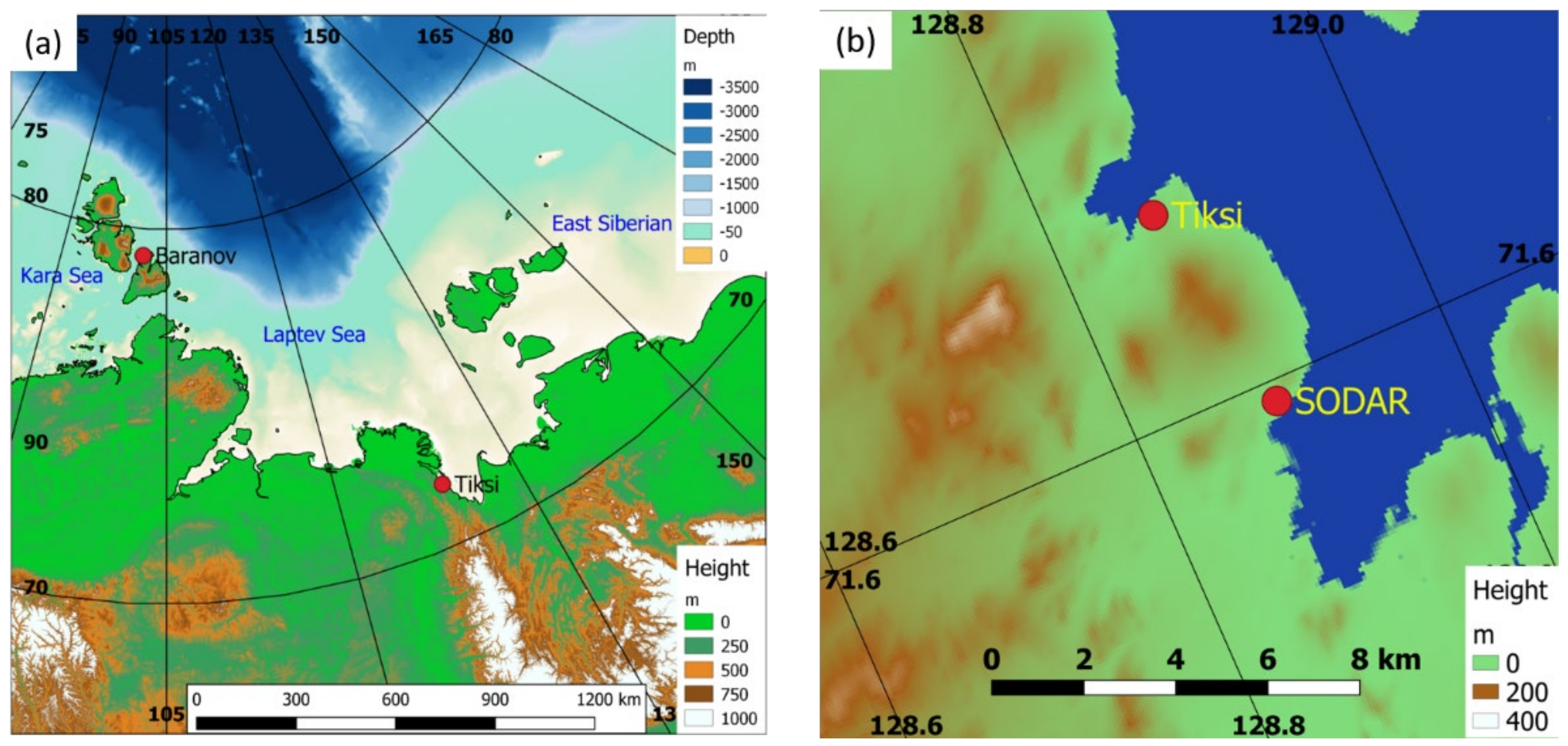
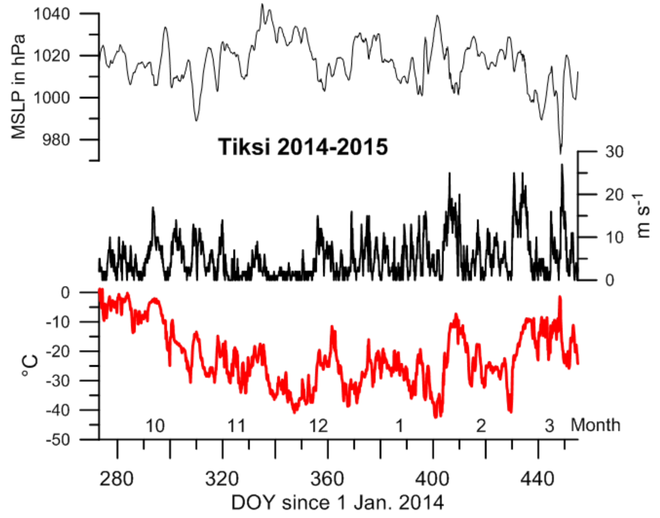
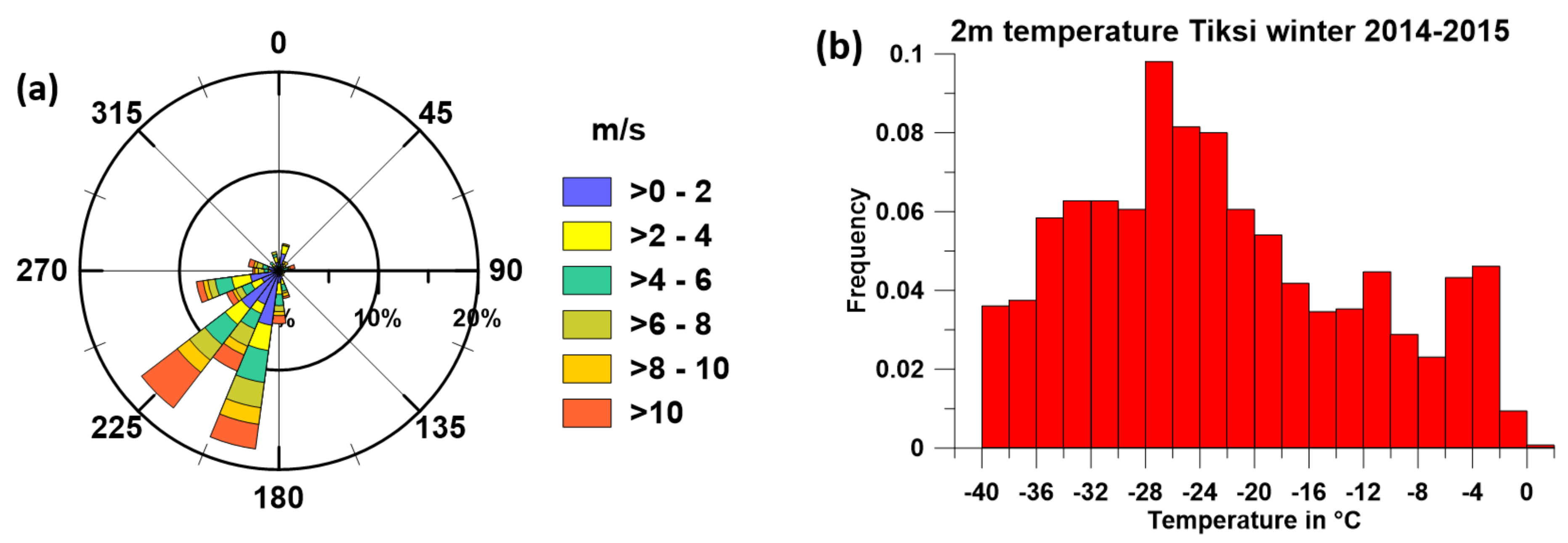
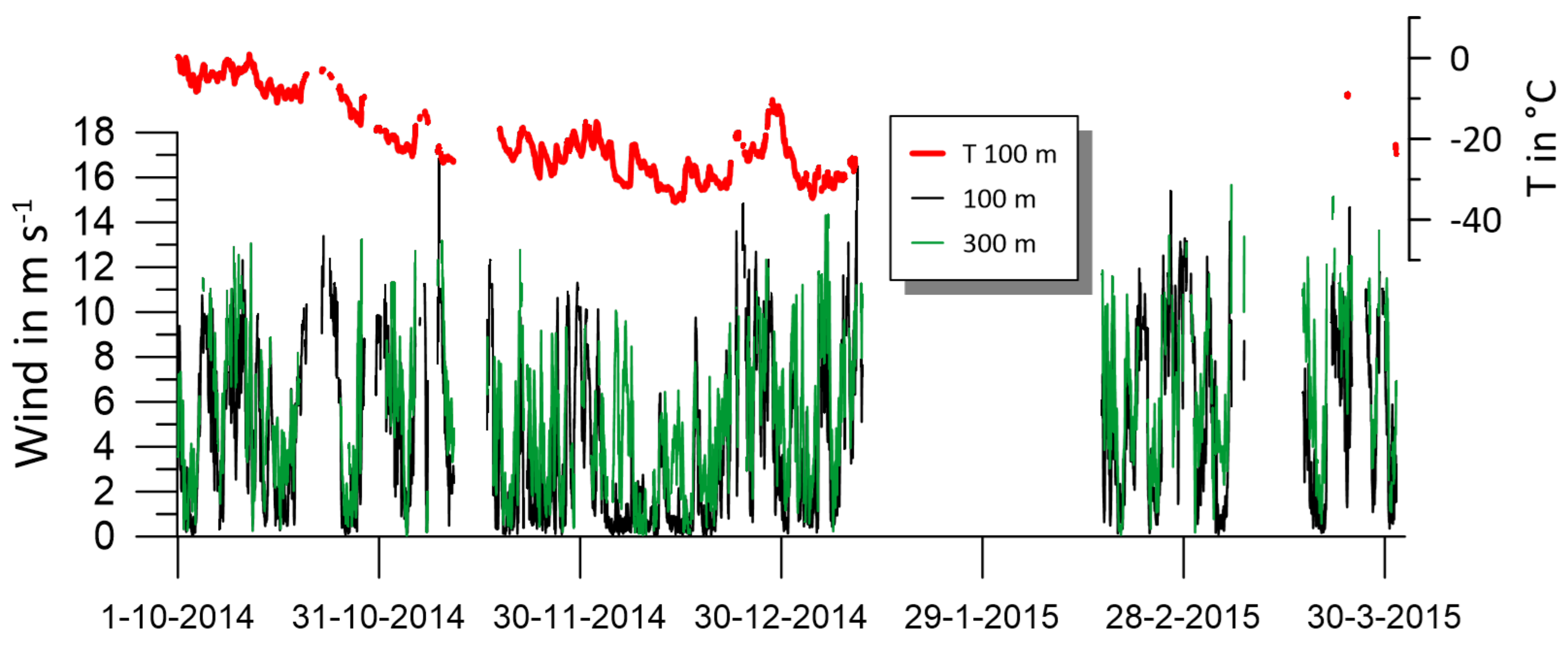
2.1. Study Area and General Meteorological Conditions
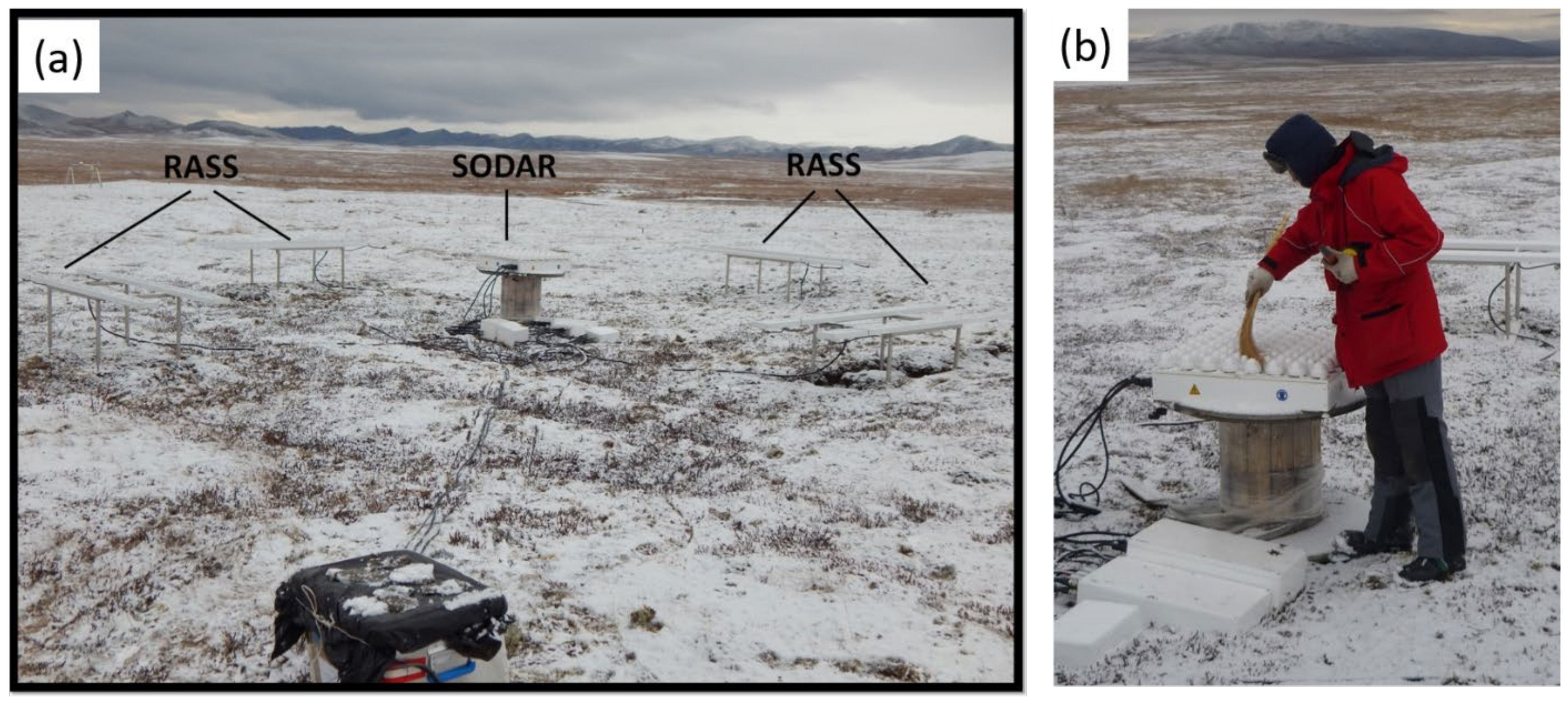
A field campaign near Tiksi in the Siberian Arctic (Figure 1a) was carried out by the University of Trier and the Arctic and Antarctic Research Institute (AARI) for the period September 2014 to September 2015. The campaign took place at the Tiksi observatory (71.60°N, 128.8°9E, 7 m asl) about 5 km south of Tiksi (Yakutia, Russia, see Figure 1b, local time: UTC+9). It is located south-east of the Lena delta at the shoreline of the Buor–Khaya Gulf of the Laptev Sea. The research motivation of the experiment was to generate a high-resolution year-round data set of the ABL structure in the high Arctic using SODAR and Radio Acoustic Sounding System (RASS) measurements for the verification of regional climate models and process studies. A special focus was on LLJs during the winter season (October–March).
In Tiksi, the temperature reaches values above the freezing point only from June to September. On average it drops below −30°C in the winter months. Fast ice begins to form in Tiksi bay in the middle of October. The average wind speeds in Tiksi are relatively high, especially during December and January with mean values above 10 m/s [20].
Figure 2 gives an overview over the meteorological conditions during the investigation period from 1 October 2014 to 31 March 2015. The mean 2 m air temperature for this period was about −23°C and stayed below the freezing point during the whole period. A strong drop of mean temperature of almost −20°C can be seen at the end of October. Minimum temperatures of −40°C and lower were measured in the middle of December and at the beginning of January, February and March. 10 m-wind speeds were high during the whole investigation period, but especially high in February and March with values of exceeding 20 m/s. The wind rose for the 10 m-wind (Figure 3a) showing that southwesterly winds were predominant, i.e. from the inland area. The 2-m temperature statistics (Figure 3b) showed a broad maximum between −18°C and −36°C.

2.2. Measurements

During the field campaign, ground-based remote sensing devices in the form of a SODAR (Sound Detection And Ranging) and a RASS (Radio Acoustic Sounding System), as well as a large-aperture scintillometer (BLS), were installed in addition to the existing instrumentation (Figure 4 and Figure 5, Table 1). Measurements of the cross-path wind speed of the BLS were used to check the plausibility of the lowest-level SODAR winds, but since we focus on LLJs and inversions, further results from the scintillometer are not presented in this paper. A SODAR measures the Doppler signal of sound returns, which are used to derive vertical profiles of the wind speed, wind direction and the turbulence characteristics in the lower atmosphere. Sound pulses, emitted by the SODAR antenna, get backscattered at temperature inhomogeneities and are then received by the same antenna (monostatic SODAR). SODAR measurements always contain information of an air volume. For the Scintec MFAS SODAR (www.scintec.com/english/web/Scintec/Details/A032010.aspx (accessed on 1 April 2021)) these air volumes have a dimension of 10 m in the vertical, and several meters horizontally depending on height. The Scintec MFAS SODAR emits at frequencies between 1650 HZ to 2750 Hz. The RASS extension (www.scintec.com/english/web/Scintec/Details/A040030.aspx (accessed on 1 April 2021)) measures the speed of sound pulses as a function of height using radio waves (frequency: 1290 MHz) and thus allows for the determination of the virtual temperature profile.
The SODAR was installed 200 m south of the Tiksi Clean Air Facility (CAF), which had a distance of about 1600 m to the main observatory, where the routine synoptic observations and radiosonde launches were performed (Figure 4). The SODAR/RASS site had a distance of about 700 m from the coastline (see Figure 4). The SODAR measurements were performed without enclosure (Figure 5), due to the fact that there are several heavy blizzards in wintertime which could have easily filled the whole enclosure with snow. Although measuring without the sound isolating enclosure, there were almost no disturbing sound sources or fixed echoes recognized by the SODAR. South of the measuring site there was a cooling system of another measuring device with a frequency of 2500 Hz. Additionally, there was a light fixed echo from the CAF. Both sources of error could be removed during the data processing. For average wind velocities near the ground exceeding 10 m/s the SODAR measurements become disturbed because the signal to noise ratio is poor [21]. Typically, wind speed measurements ranged from 30 m to 560 m (10 m vertical resolution) and temperature measurements from 40 m to 250 m (10 m vertical resolution).
The maximum range of the RASS measurement was 250 m and decreased with increasing wind speed (which is typical for a monostatic SODAR/RASS). Complete data loss for the RASS occurred for near-surface wind speeds exceeding 10 m/s. Another problem was the alignment of the RASS antennas, which has to be exact for the RASS to function properly. Unfortunately, the only grounding available was hand-build stone piles, since the soil consists of shale chips that cannot be dug into without machinery, which is not permitted in summer for environmental protection (see also Figures S3 and S4 in the Supplementary Materials). In consequence, the alignment was lost during the annual freeze cycle and the RASS signal was lost in spring. Time resolution for RASS and SODAR profiles was set to 20 min.
If the SODAR/RASS raw data pass the quality control they are processed to raw wind measurements that can be used for further evaluation. To guarantee the quality of these data, additional control mechanisms available in the Scintec SODAR software have been applied; for example, a confidence level based on the spectral shape of the echo and a temporal and spatial consistency check of wind speed and direction. The SODAR/RASS wind and temperature data were then also checked against the tower, scintillometer and radiosonde data for credibility. This comparison revealed that–probably due to the missing acoustic enclosure–spurious low wind speeds were found above the actual current range of the SODAR, for example in case of strong elevated inversions. To eliminate these errors in the wind profile, additional quality checks were introduced based on the vertical gradient of the wind speed and variance of the vertical wind component.
The available SODAR/RASS data set for October 2014 to March 2015 is shown in Figure 6 as the time series of the wind speed at 100 m and 300 m and temperature at 100 m. A small data gap can be seen from 11 to 16 November 2014, but a larger failure of the SODAR occurred from 11 January to 16 February 2015 and at the beginning of March. The RASS worked well until mid of January, but failed almost totally for the rest of the measurement period. It is also obvious that in many cases the wind speed at 100 m is larger than the wind speed at 300 m indicating an LLJ. Overall, the data availability of the SODAR at 100 m is 62% for the whole winter. The quality checks led to a reduction of the wind data for the upper levels relative to 100 m (89%, 80% and 66% for 200, 300 and 400 m, respectively).
Table 1 summarizes the meteorological instrumentation during the investigation period. For the present paper we use only data of SODAR/RASS and the tower near the CAF site, the standard synoptic observations and radiosondes at the observatory, and data of the Baseline Surface Radiation Network (BSRN) station [22,23].

2.3. Numerical Model Data

Numerical weather forecast data are used to study the synoptic environment. The non-hydrostatic regional climate model COSMO-CLM (CCLM, [24]) was used to produce a high-resolution atmospheric data set. The model is nested in ERA5 data and uses high-resolution sea ice concentration data [25] on a daily basis to keep the hindcast close to reality. CCLM was adapted to the polar regions by the implementation of a thermodynamic sea ice model ([26,27,28]). The model was run for the whole Arctic with a resolution of 15 km [29,30]. Data is available every hour.

3. Low-Level Jets and Detection Criteria

There are different mechanisms for the formation of LLJs:
  • Inertial oscillation: stable stratification leads to a strong decrease of turbulence inducing a decoupling of the upper layer of the SBL as friction becomes negligible. The resulting imbalance of Coriolis and pressure gradient forces causes a super-geostrophic wind by an inertial oscillation [2,31,32,33,34].
  • Baroclinity causes a vertical shear in the geostrophic wind [11,16].
  • Katabatic winds forming in the SBL over sloped terrain are typically associated with LLJs [13,35].
  • Topographic channeling and local density flows [6,15,36].
  • Offshore LLJ due to a decrease of friction from rough land to smooth water or sea ice surfaces [37,38].
The inertial oscillation LLJ is the most frequent LLJ at mid-latitudes (nighttime LLJ). It can be seen in hodographs and the duration of a LLJ event is limited to some hours depending on the period of the inertial oscillation. This period is about 12.6 h for the latitude of Tiksi. While the nighttime inertial oscillation LLJ is caused by the formation of the surface inversion in the evening, the decoupling of the upper layer during the polar night can also result from warm air advection or by changes from cloudy to clear conditions. Ref. [37] refers to these LLJs in a more general sense as thermal boundary layer jets. LLJs associated with katabatic winds do not develop in the Tiksi area, but topographic effects can occur. Topography rises to an elevation of about 200 m north-northeasterly of the SODAR/RASS (Figure 4), which may influence the wind in the lower 200 m. The distance to the foot of this hill is about 900 m (see Supplementary Materials for more maps). The effect of the topography could be a flow over and around the hills, depending on the Froude number. An overflow over the hill north of the measuring site (during northerly winds) can cause increased turbulence due to gravity waves. A flow around this obstacle (during westerly or easterly winds) can cause increased wind speeds in the lower 200 m due to channeling effects. When we compare the wind statistics at 100 m and 400 m (Figure 7a,b) a shift to more southwesterly and southeasterly directions can be seen, possibly indicating the impact of topography on the flow. The observed low-level jets (LLJs) (see Section 4 for details) are almost exclusively from westerly (Figure 7c).
By means of the SODAR data it is possible to detect LLJs within the SBL. [39] identified LLJs by visual inspection of horizontal wind speed, variance of vertical velocity and acoustic backscatter intensity profiles of SODAR measurements. [2,40] defined a LLJ as local wind speed maximum that is 2 m/s higher than the next minimum below and above. [4] used the same definition, but with 1.5 m/s difference of the local wind speed maximum and the next minimum below and above. [41] defined the jet core height as the height of the maximum wind speed which is at least 25 % and 2 m/s faster than the next minima. This definition prevents a false classification at very low wind speeds (absolute criteria) and at very high wind speeds (relative criteria). The oldest LLJ classification is from [42], who had chosen four criteria to determine low-level jets. His weakest criteria defined LLJs as any jet speed maximum within the first 1500 m above ground with a decrease of at least 3 m/s above the maximum.
In this study we use the LLJ definition according to [2], which detects all LLJs regardless of the wind speed (the minimum must exceed 2 m/s according to the definition). Within the detected LLJs, we use an additional threshold for the jet speed of 10 m/s for strong LLJs. In order to increase the coverage of LLJ detection due to the lack of the vertical height range of the SODAR, one-hourly averaged wind speed profiles were used. In the case of a gap between two hourly profiles, a check for temporal consistency was included as an additional criterion. If a LLJ could be detected in the prior and the following hourly profile, we assume that the jet event is also present at the actual hour. As a result of this kind of gap filling, additional 61 (general LLJ definition) and 5 (strong LLJ definition) hourly profiles with LLJs were detected. The relative frequency of LLJs was calculated as the ratio of the number of counted LLJ profiles and the number of observations.

4. Results

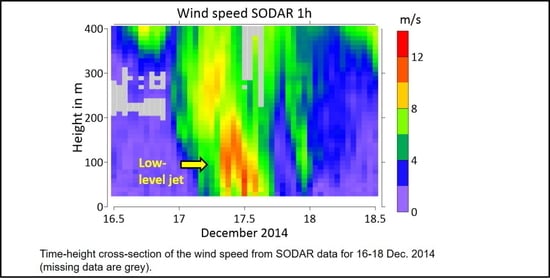
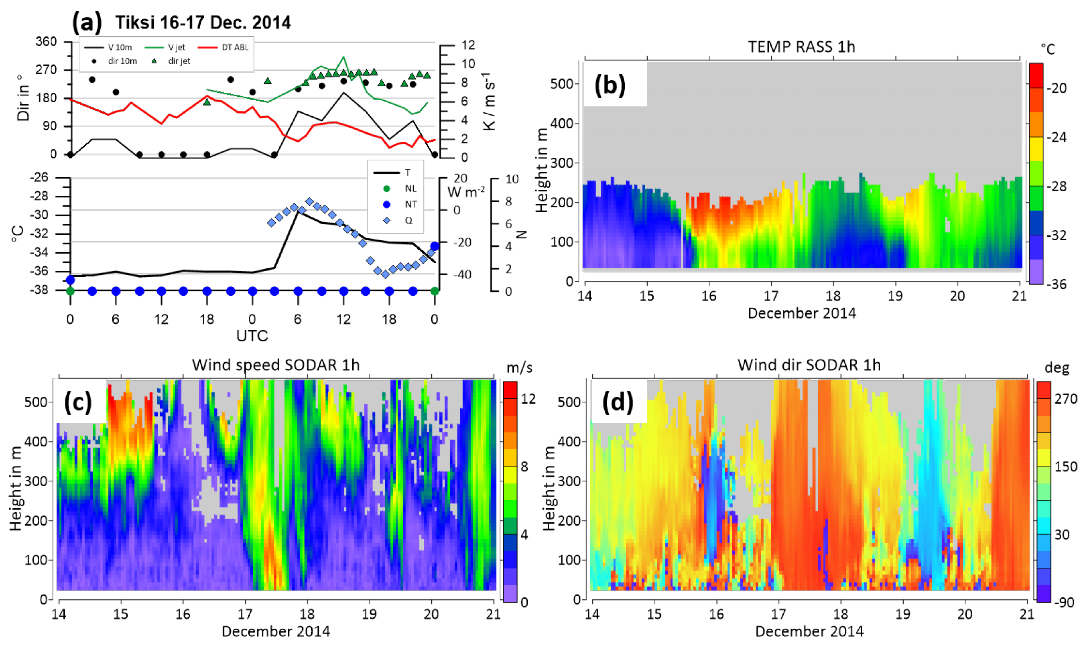
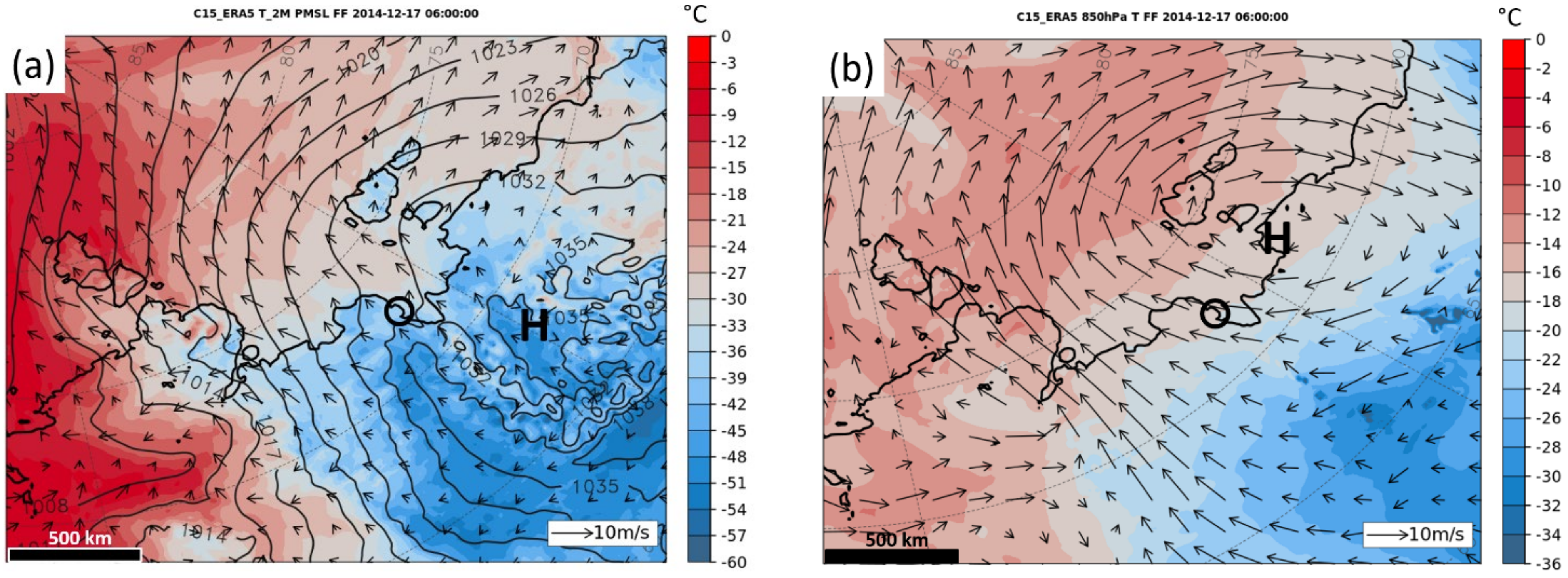
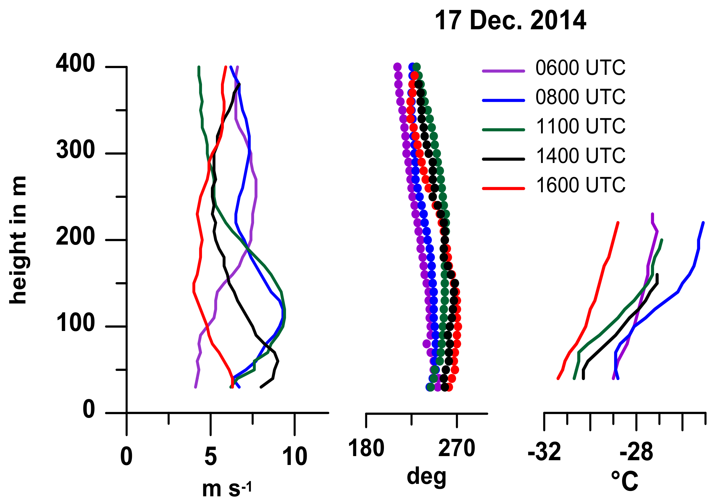
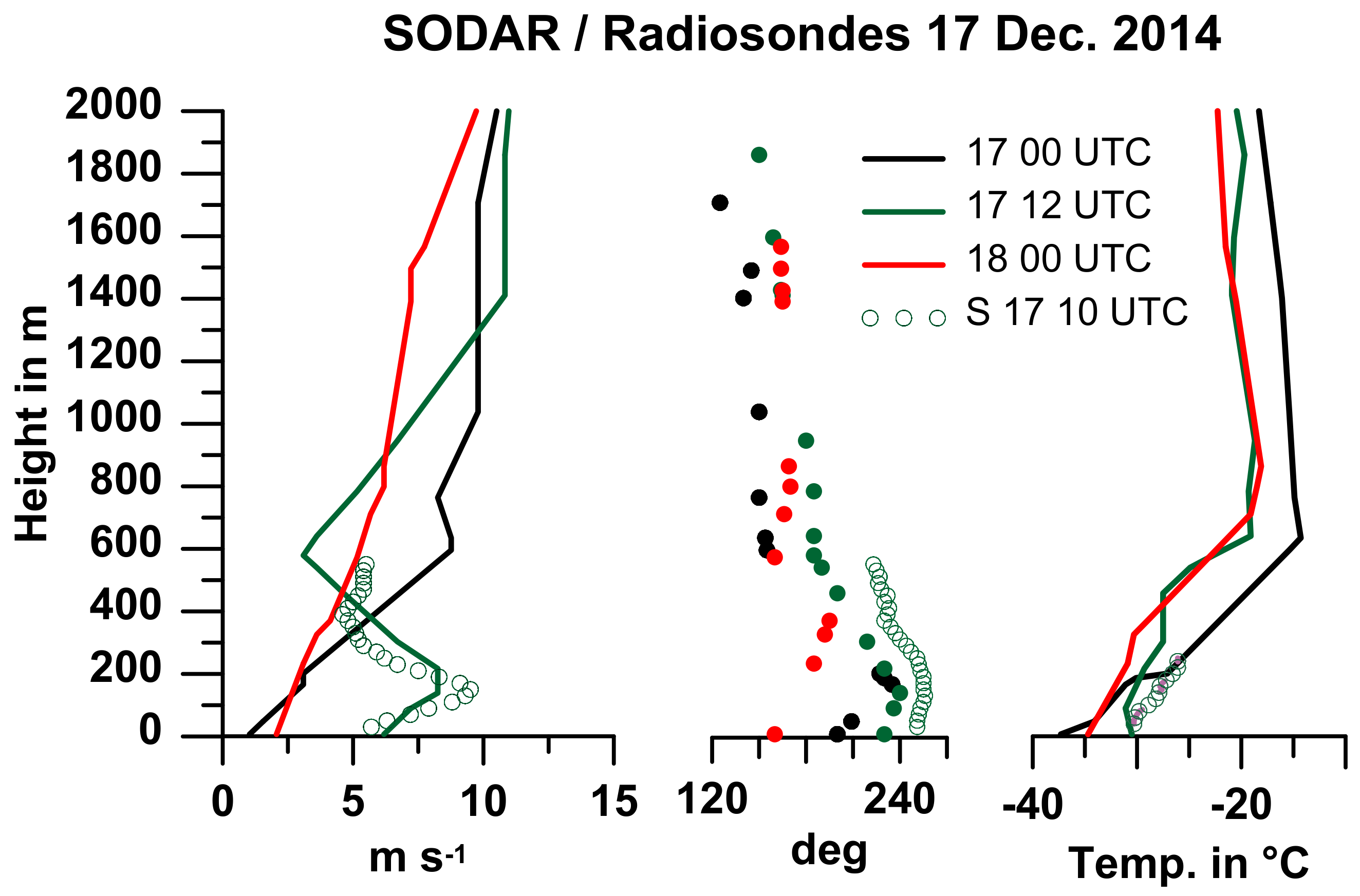
4.1. Case 17 December 2014

During the period from 14 to 21 December 2014 several LLJ events occurred (Figure 8). During the first two days, strong winds are present above 400 m, but the range of the SODAR does not allow to detect these as LLJs. On 17 December and later on, a very shallow strong LLJ and a number of weaker jets can be seen. In the following, we focus on the LLJ on 17 December 2014.
On 16 December very weak winds with temperatures around −36°C prevail near the surface (Figure 8a), followed by a warming with the onset of medium winds from southwest at the beginning of 17 December (0000 UTC corresponds to 1000 local time), but then a cooling and decrease of net radiation occurs throughout 17 December and the wind decreases again. No clouds were observed during this period. The RASS data (Figure 8b) show a stable stratification for all days, which is most-pronounced on 16 December and gets weaker with the onset of the LLJ. This LLJ develops during 17 December and has a shallow core around 100 m (Figure 8c) with maximum wind speeds of more than 10 m/s. The wind direction at the jet core was around 240° (Figure 8d). The vertical shear in wind direction is relatively small. This can be also seen in the comparison between the synoptic observations near the surface and the wind from SODAR at the jet core (Figure 8a). The course of the ABL stability (given by the temperature difference between 200 m and 40 m as from RASS data) shows a decrease during the onset of the LLJ (Figure 8a). The turbulence associated with the LLJ (derived from SODAR wind variance and backscatter data, not shown) was quite strong and is a likely reason for the stability decrease. Two weaker jets at about 200 m and 300 m can be seen on 19 December and 20 December, respectively. The jet on 19 December is associated with northeasterly wind directions, while the jet on 20 December is southwesterly.
The synoptic situation for the onset of the LLJ on 17 December is shown in Figure 9 for 0600 UTC on 17 December. A high-pressure system is located over the Siberian land mass southeast of Tiksi and cold air is advected from the interior of Siberia towards the Laptev Sea (Figure 9a). In the region of Tiksi, there is a strong temperature contrast at low levels between the cold land and the warmer (sea-ice covered) Laptev Sea. At 850 hPa (Figure 9b), the high is northward compared to the position at the surface, but also here we find cold air advection and baroclinicity for the Tiksi area.
The vertical profiles on 17 December show the LLJ evolution in detail (Figure 10). At 0600 UTC the wind speed was still low in the lowest 100 m and had values of about 4 m/s. Above 200 m the wind had already increased to values of 7–8 m/s with no pronounced wind maximum (see also Figure 8c). The LLJ developed very quickly between 0600 and 0800 UTC with about 10 m/s wind speed and a jet height of about 100 m. The wind direction remained almost constant during the development. The LLJ began to weaken in the afternoon and had disappeared at 1600 UTC. The wind direction showed a slight turning to more westerly directions, but a small directional shear with height for all profiles. The temperature profiles showed the strong stability of the SBL and the overall cooling during the day.
Radiosondes were available for 0000 and 1200 UTC for this period. Due to the short lifetime of LLJs, only few of them were detected in the operational radiosoundings. Since the LLJ on 17 December occurred between 0800 and 1400 UTC, the radiosonde data can be used to study the atmospheric structure also at larger heights. The comparison of the SODAR/RASS data with the radiosonde profile at 17 December 1200 UTC shows good agreement (Figure 11). Due to the much higher resolution, the LLJ was more pronounced in the SODAR data. For the wind direction and temperature, there is a slight positive bias for the SODAR/RASS data compared to the radiosondes, but it should also be considered that the radiosonde drifts with the wind and the difference in position between SODAR and radiosonde increases with increasing height (the distance between SODAR and the position of the radiosonde launch is already about 1600 m). The radiosonde data show that the surface inversion extends up to 600–800 m throughout the day. The veering of the wind extends up to 2 km, i.e. the wind direction is southeasterly at larger heights (consistent with the 850 hPa map of Figure 9b) and shifts from southerly to southwesterly and back in the lowest 200 m. Since the inversion top was higher than jet core height, an influence of hills with elevations of about 200 m north and 120 m west of the measurement site (Figure 4) is likely.
An LLJ caused by an inertial oscillation should be seen in hodographs. The period of the inertial oscillation is about 13 h for the latitude of Tiksi. The hodograph at the height of the LLJ on 17 December is shown in Figure 12a. The LLJ results mainly of the increase of the westerly wind (positive u) between 0600 and 0800 UTC. No indication of an inertial oscillation can be seen.

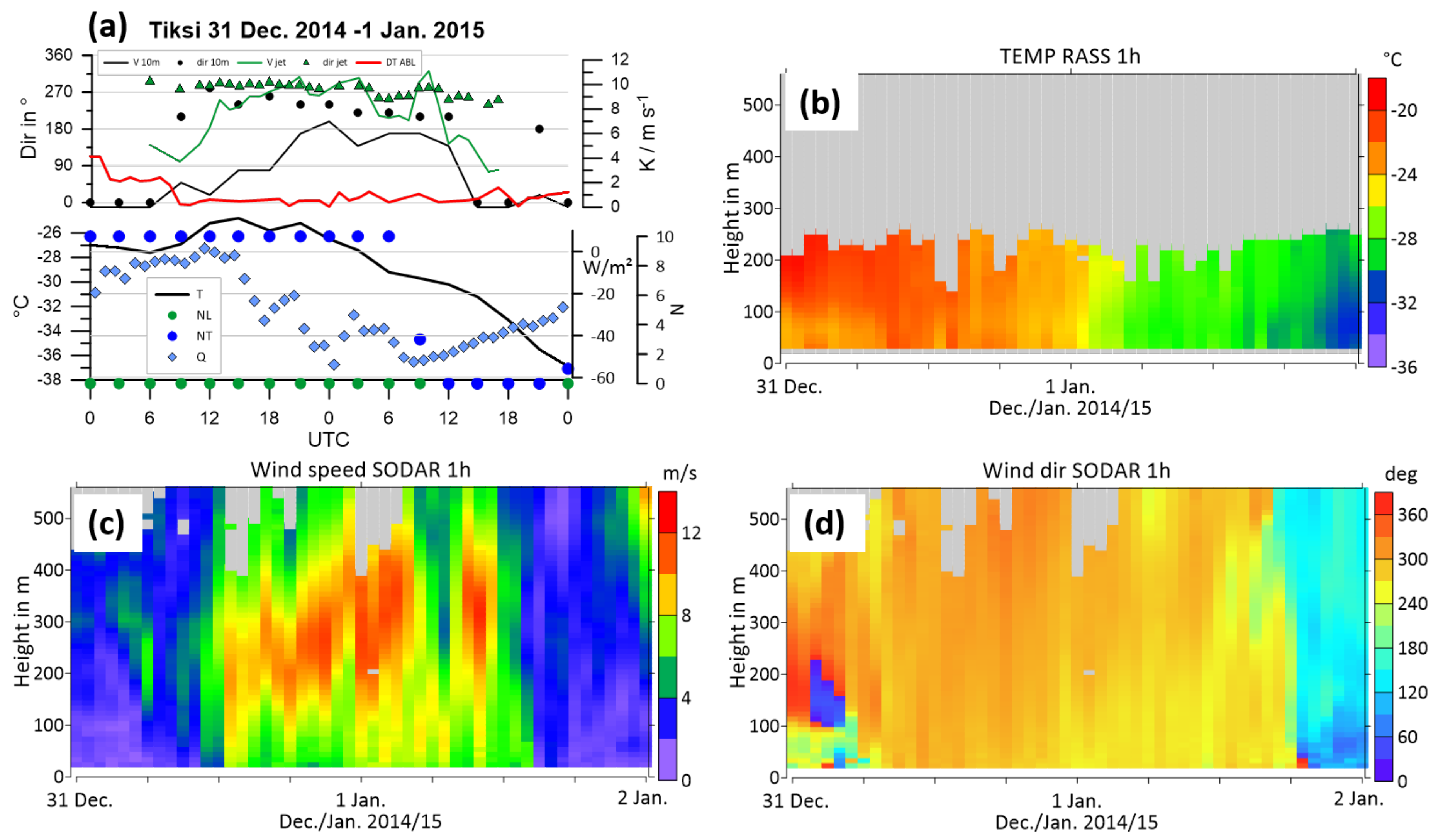
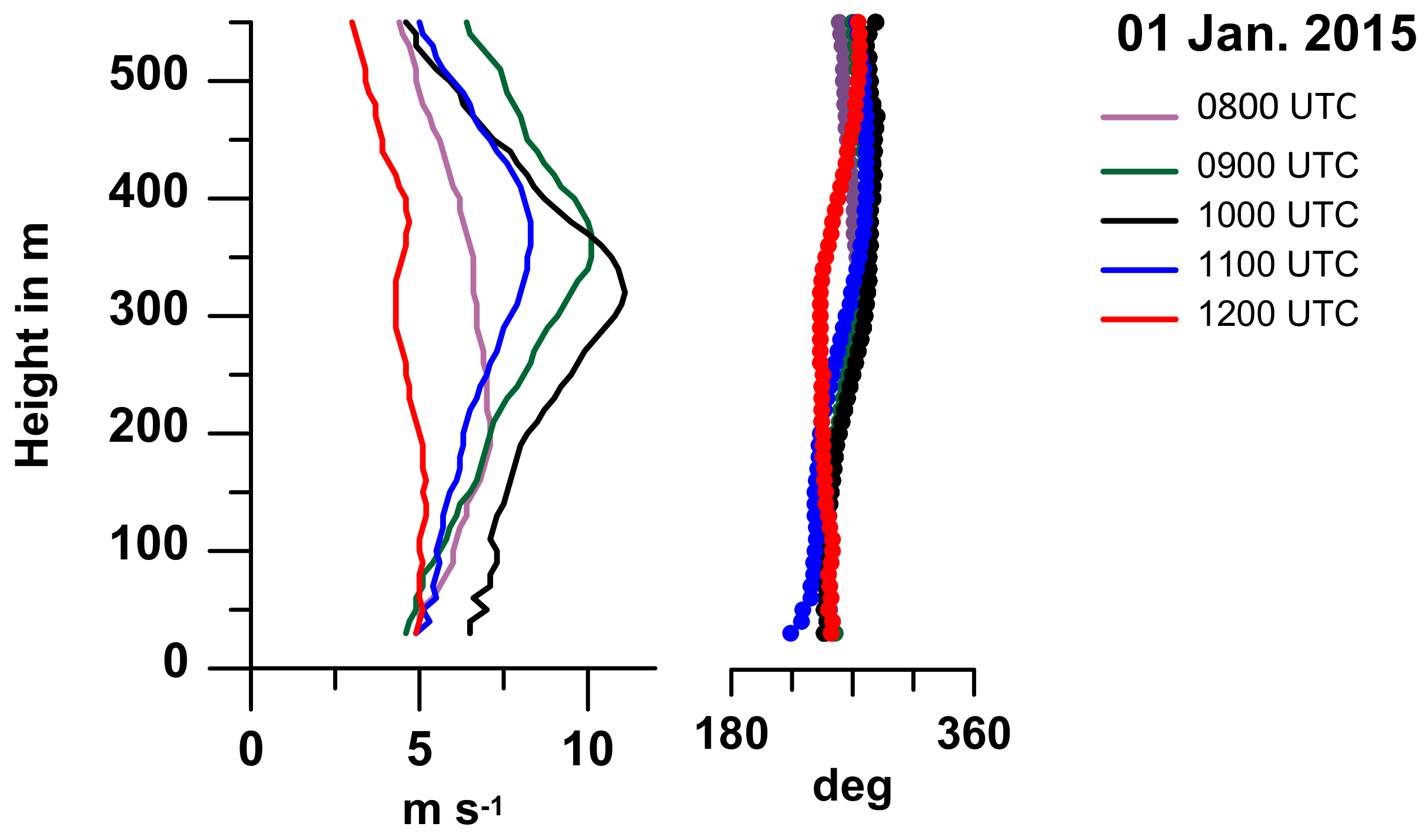
4.2. Case 1 January 2015

During the period 31 December 2014 to 1 January 2015 a LLJ event with a very long duration of 30 h occurred (Figure 13). 31 December started with a calm period for the 10 m-wind, but a weak LLJ from westerly directions was observed for a few hours (Figure 13a,c). In the late morning of 31 December the near-surface wind changed to westerly directions and increased to 6 m/s (Figure 13a). This was associated with a decrease of the net radiation during the second half of 31 December 2014, and only high or mid-level clouds were observed. On 1 January 2015 a cooling of about 10 K took place, while the wind dropped to low values at about 1200 UTC. The cooling can be seen throughout the lowest 200 m (Figure 13b) and the part of the SBL in the range of the RASS data was only weakly stable (Figure 13a). The period of high near-surface winds corresponds to the wind structure from the SODAR (Figure 13c). The LLJ started at 1200 UTC on 31 December 2014 and lasted until 1800 UTC on 1 January 2015. The jet core intensified on the second half of 31 December and rose from 200 m to 300 m. After a couple of hours with weaker winds, the LLJ intensified again with winds exceeding 10 m/s until 11 UTC on 1 January 2015. For the whole period of the LLJ the wind direction in the jet core was westerly to northwesterly (Figure 13a,d). The profiles of the LLJ event on 1 January are shown in Figure 14. The jet was most pronounced at 1000 UTC and can be classified as strong jet (exceeding 10 m/s). The hodographs at the height of the LLJ on 31 December (Figure 12b) and 1 January (Figure 12c) showed again no inertial oscillation, but mainly the increase and decrease of the westerly wind (positive u). Since wind profiles from radiosonde ascents were only available at 1200 UTC on 31 December 2014 and 1 January 2015, the LLJ event was not captured by the radiosondes.

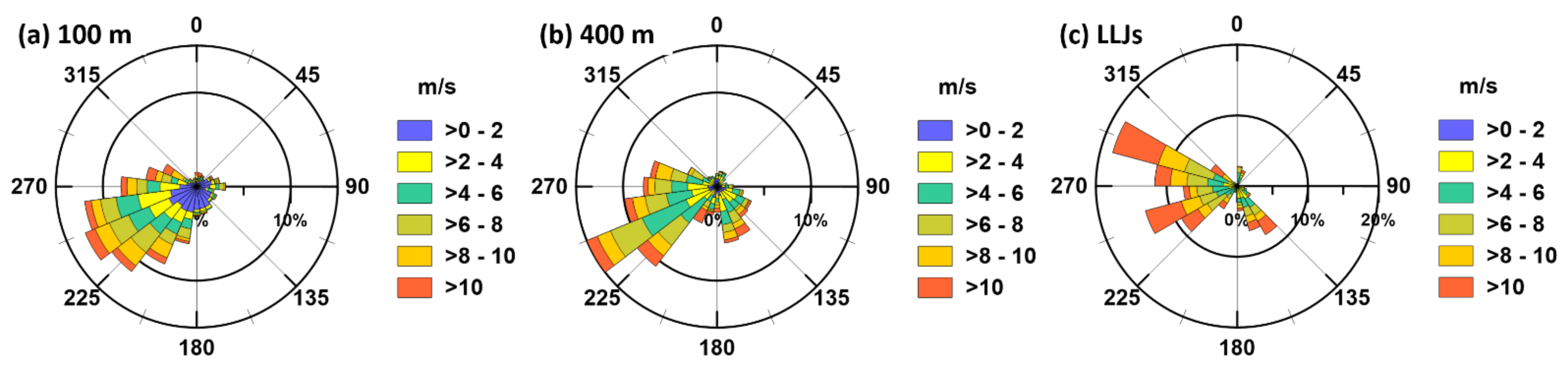
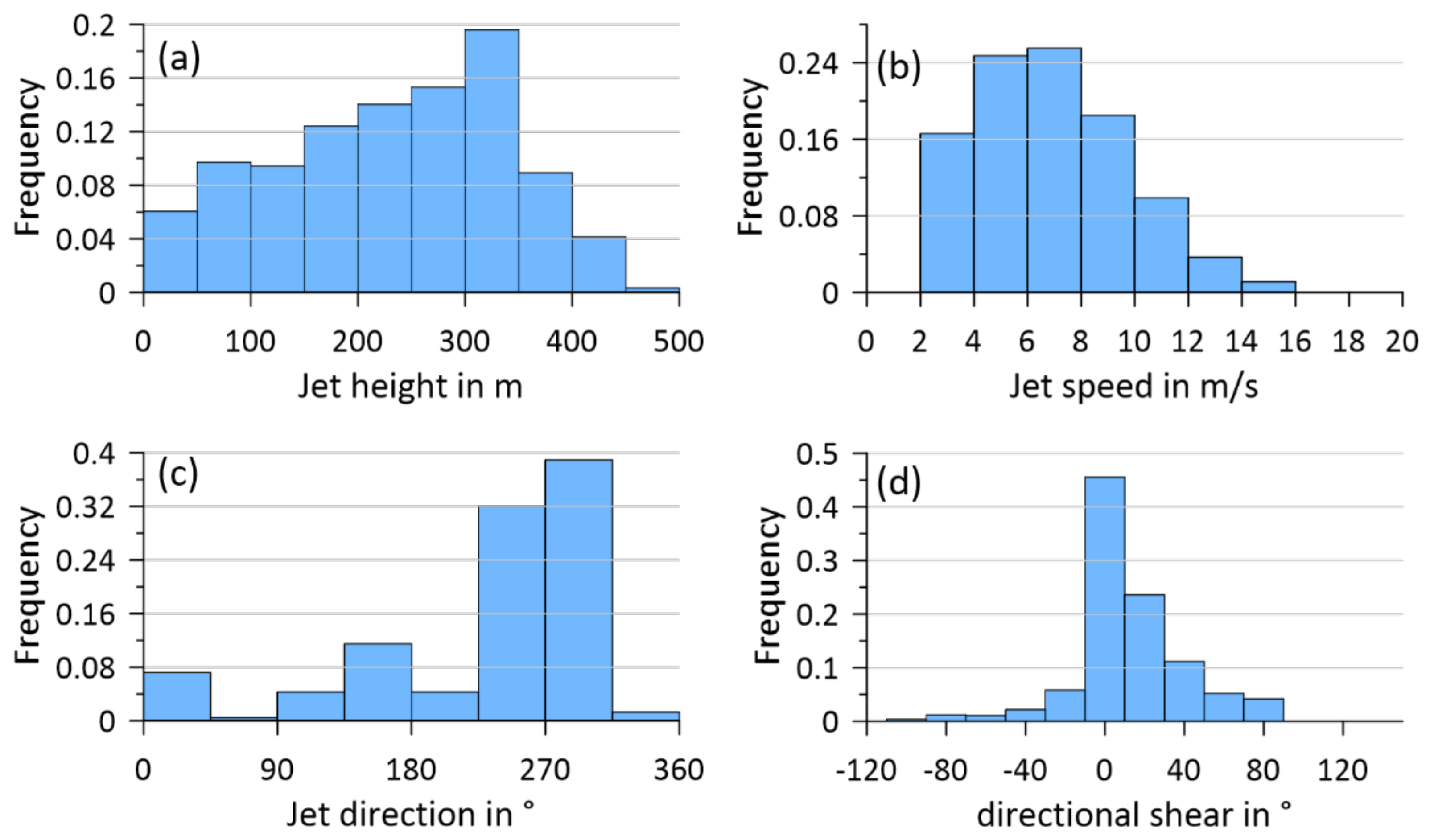
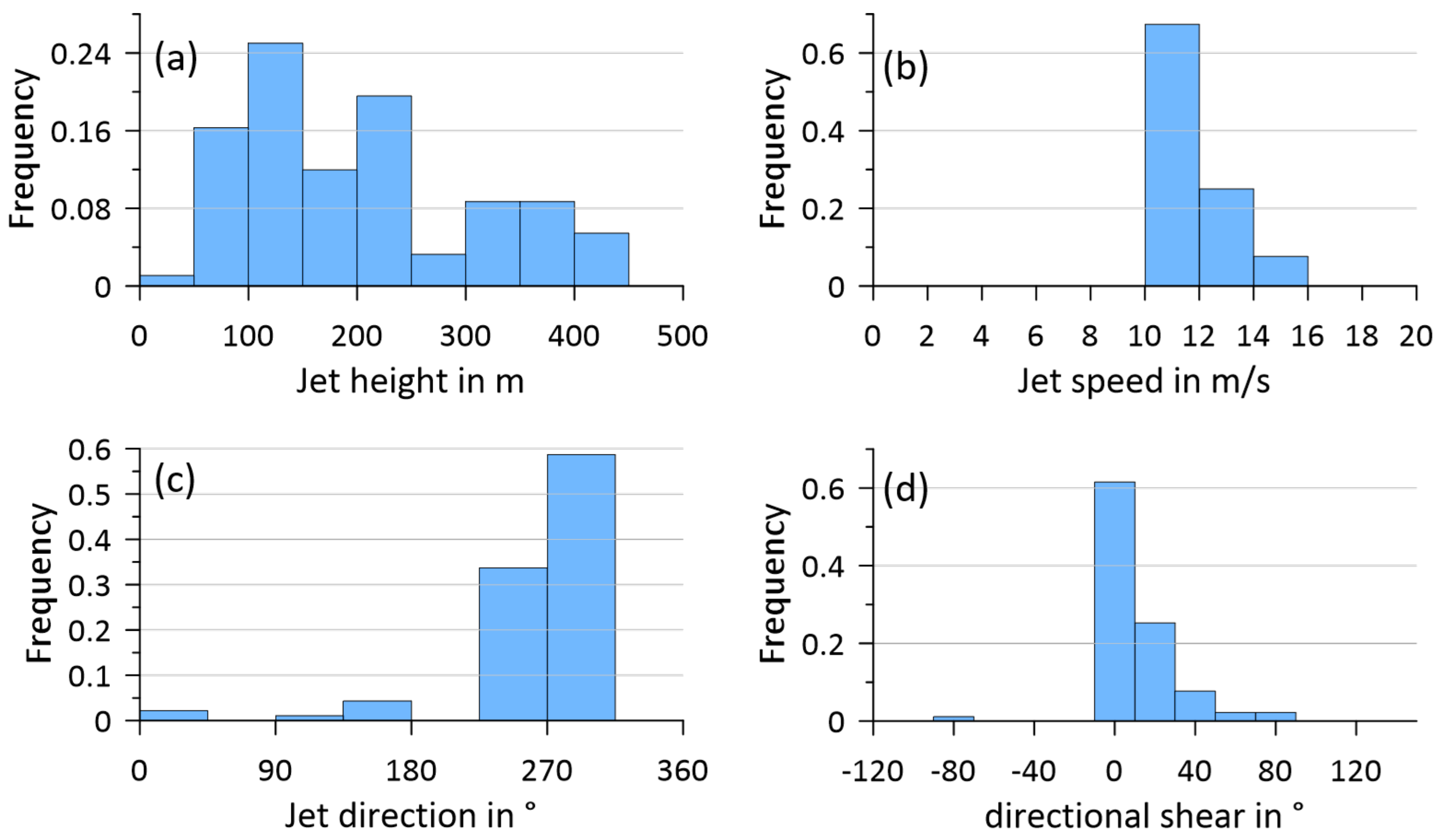
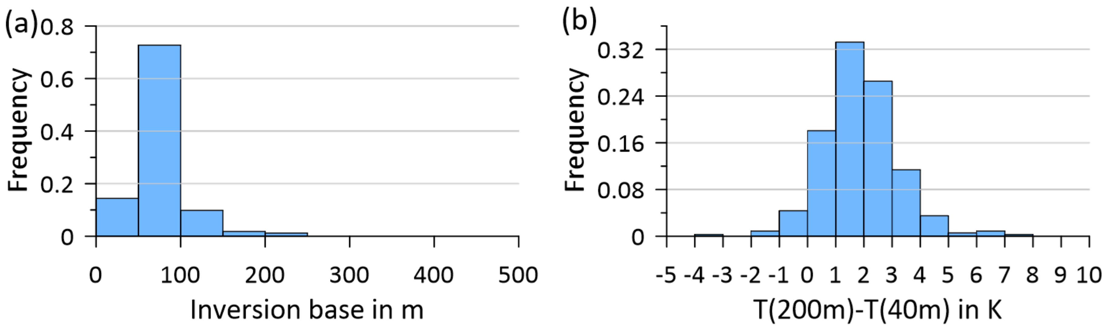
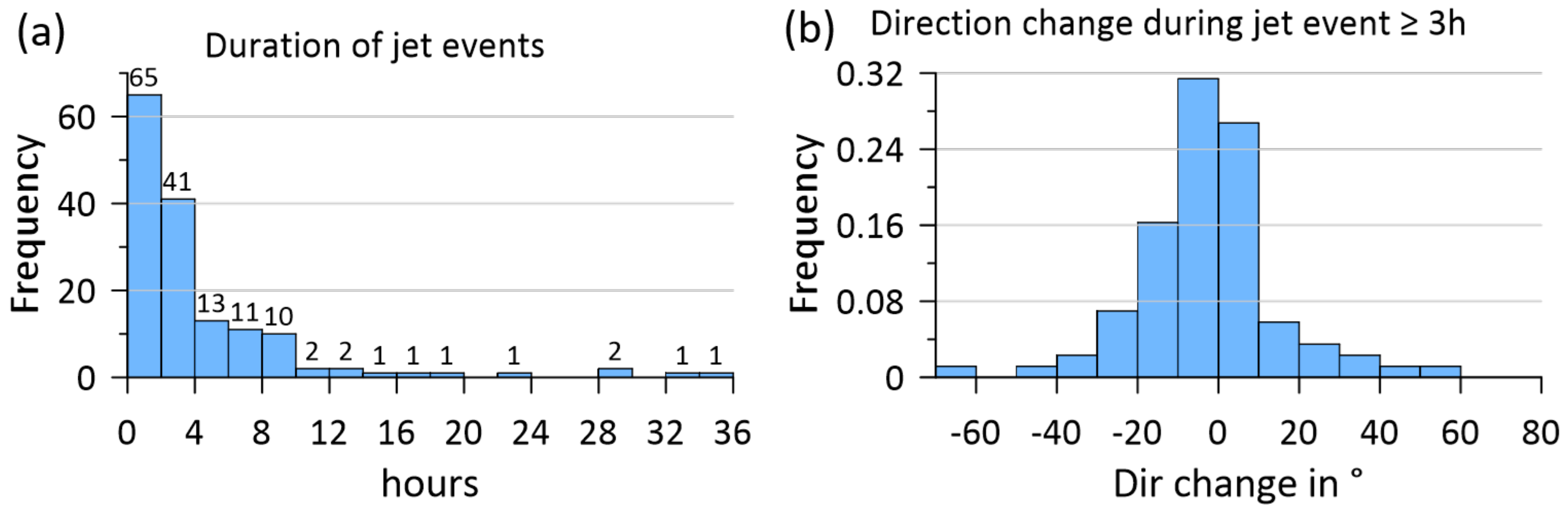
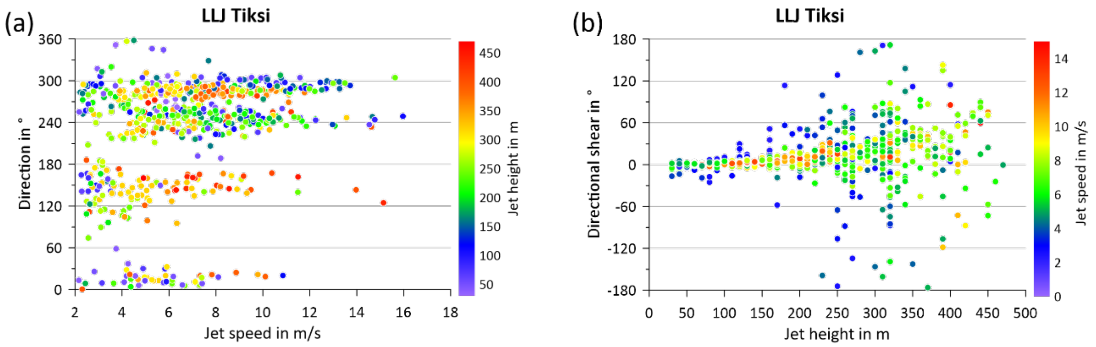
4.3. Statistics of LLJs for Winter 2014/2015

The here presented results refer to the period from 1 October 2014 to 31 March 2015. At a height of 50 m above ground, the wind and temperature measurements show a data availability for this period of about 67% and 49% of the SODAR and RASS measurements, respectively. At 200 m above surface the data availability was 64% and 47%, respectively. At 500 m the data availability for the SODAR was 48%. A stated in Section 2, RASS measurements were limited to 250 m and near-surface wind speeds below 10 m/s and are only available until January 2015.
The statistics for all LLJs are shown in Figure 15 and for strong LLJs in Figure 16. A total of 2690 1 h-profiles were measured. LLJs were detected in 627 profiles (all LLJs) and 92 profiles (strong LLJs), respectively. Thus, LLJs occurred in 23.3% of the profiles, and strong LLJs in 3.4%. The highest frequency for the jet height was found at 300–350 m for all LLJs, while strong LLJs were most frequent at 100–150 m. The average jet heights were 236 ± 109 m (all LLJs) and 205 ± 107 m (strong LLJs), respectively. Strong LLJs were almost exclusively westerly, and for all LLJs a second (but weaker) maximum was found from southerly directions (see also Figure 7c). Directional shear between low levels and the jet core was very small for strong LLJs. For all LLJs, larger directional shear was found for some cases, and there were also more negative values compared to strong LLJs. A positive shear can be expected due to friction due to Ekman dynamics. The average jet speed was to 6.9 ± 2.8 m/s (all LLJs) and 11.7 ± 1.4 m/s (strong LLJs) with a maximum jet speed of 16.0 m/s. Since the inversion tops were measured only in few cases, we analyze the static stability of the lowest 200 m (taking the tempera­ture difference between 200 m and 40 m as well as the height of the inversion base from RASS data (Figure 17). The inversion base could be detected in 52% of the LLJ profiles, the temperature difference was available for 55% of the profiles. The inversion base was found between 50 and 100 m for most cases. The temperature difference distribution shows that stable stratification was present for almost all LLJ profiles (note that the difference is −1.4 K for adiabatic conditions). The mean difference was 1.9 ± 1.3 K, corresponding to a mean temperature gradient of 1.2 K/100 m (the maximum is 4.4 K/100 m).
The statistics of the LLJ event durations is shown in Figure 18a. A LLJ event is defined as the period where in consecutive profiles the LLJ criterion is fulfilled. The highest frequency was found for LLJs with a short duration (1 h), but the majority of LLJs had a longer duration of 3 to 10 hours. The LLJ events detected only as a single 1-h profile are suspected to fall into the class of turbulence-generated wind maxima [12]. However, we have reduced these fluctuations by averaging three 20-min-profiles. From these short events, 66% had maximum speeds of less than 8 m/s, and the absolute detection criterion of at least 2 m/s wind speed decrease above and below the jet exceeds the relative criterion of 25%, which [12] defined to exclude turbulence generated wind maxima.
The discussion of the case studies has shown that no indication of an internal oscillation was found. We extended this analysis to all LLJs with at least 3-h duration by looking at the change in wind direction between the end and the start of an event (Figure 18b). The highest frequencies were found for ±10°, that is, no change. Larger directional changes were found with both signs, with a slight bias to negative values (wind turning counter-clock wise during the event). An internal oscillation would lead to a clockwise change in the wind direction. It was also tested if there was a stability increase 6 h prior to the jet development (see Figure S6 in the Supplementary Materials). The statistics show that there were both decreases and increases mainly in the range of ±2 K for the temperature difference between 200 and 40 m prior to the jet development for LLJs events of at least 3-h duration. However, there is a bias to a near-surface cooling 6 h prior to the jet development (see Figure S7 in the Supplementary Materials).

5. Discussion

In the present study, LLJ characteristics are investigated for a whole winter season in a coastal area of the Siberian Arctic. Only few long-term studies of LLJs are available for high latitudes. The model-based climatology of LLJs for the wintertime Arctic by [12] shows LLJ frequencies around 20% for the inner Arctic including the Laptev Sea. Their LLJ definition is based on the same absolute criterion of 2 m/s anomaly as in the present study, but they use a relative criterion of a 25% decrease above and below the wind maximum in addition. In the present study, LLJs were observed in about 23% of all profiles and on 68% of all measurement days at Tiksi in the winter season October 2014 to March 2015. [11] analysed LLJs over the central Arctic Ocean during April to August 2007 taking data from tethersonde soundings of the drifting station “Tara”. They found LLJs in 46% of the observations, and baroclinicity was found to be the most important mechanism (about half of the LLJs were associated with the passage of fronts). [2] investigated LLJs in the Weddell Sea of the Antarctic during the fall/winter season by means of tethersondes using a similar LLJ definition as in our study. They found LLJs in 80% of the profiles, which were mostly associated with inertial oscillations due to synoptic-scale changes in stratification. Their statistics of jet height and jet speed showed highest frequencies around 100 m and 6–8 m/s, respectively. Thus, the speed distribution is similar, but the jet heights are much lower compared to our study. On the other hand, they detected inversions at larger heights than in our study. Their directional shear between the near-surface wind and the LLJ was consistent with Ekman dynamics with most frequent values of around 30 degrees. In contrast, our study shows a clear peak for no directional shear and only some cases were consistent with Ekman dynamics. [43] studied LLJs using Doppler lidar measurements for about two years on a small island in the northern Baltic Sea (60°N). LLJs were identified in only 12% of the profiles. Most LLJs were lower than 150 m, and the mean jet speed was 11.6 m/s. A strong seasonality was found with highest values during summer (30%) and lowest values during winter (<5%).
As discussed for Figure 17, a stable stratification is present for all LLJs in the lowest 200 m, which is also the height of the surrounding hills in the vicinity of the SODAR/RASS. In Figure 15 and Figure 16 it has been shown that all jets had the highest frequency for westerly directions, and that strong LLJs have lower heights. Figure 19a shows the relation between jet speed, direction and height in a different way. Again, we see the majority of LLJs from westerly and a second maximum for southerly directions. Almost all LLJs with a height lower than 200 m were in the westerly sector, particularly for the stronger LLJs. The relation between jet height and directional shear (Figure 19b) shows that the directional shear (difference in wind direction between jet and near-surface) was very small for jet heights below 200 m (for all jet speeds). For jet heights larger than 300 m the scatter becomes large. This indicates that the hills around the Tiksi observatory may influence the flow in the lowest 200 m.
Our observations have shown that the inertial oscillation being associated with a thermal boundary layer jet [37] was not found in our cases. While strong changes in the stability of the boundary layer occur also during the polar night leading to a decoupling of the upper layer of the SBL, this effect seems not the dominant one. The main driving mechanism of LLJ events seems therefore to be baroclinity, which may result from the strong low-level temperature gradient between land and the sea-ice covered ocean, but also from temperature advection. [33] discussed also the role of temperature advection and katabatic winds superimposed on a strong surface inversion as factors for generating LLJs in fjords.

6. Conclusions

The present study yields new information about LLJ characteristics for a whole winter season (October 2014 to March 2015) in the remote area of the Siberian Arctic and provides a data set for the verification of weather forecast and regional climate model data. The statistics of LLJs for six months show that in about 23% of all profiles LLJs were present with a mean jet speed and height of about 7 m/s and 240 m, respectively. In 3.4% of all profiles LLJs exceeding 10 m/s occurred. LLJs were observed on 68% of all measurement days at Tiksi in the winter season. There seem to be several complementary mechanisms leading to the LLJ formation and structure. The main driving mechanism for LLJs seems to be the baroclinicity, since no inertial oscillations were found. LLJs with heights below 200 m are likely influenced by local topography. High-resolution modelling is needed to understand the processes of the LLJ dynamics in more detail.

Supplementary Materials

The following are available online at https://0-www-mdpi-com.brum.beds.ac.uk/article/10.3390/rs13081421/s1: Figure S1: Map of the investigation area with positions of the SODAR, the clean air facility, the micro-meteorological tower and the main observatory. Figure S2: Zoom-in of Figure S1 as 3D view. Figure S3: Photo of the phased-array antenna of the SODAR. Figure S4: Photo of the SODAR/RASS installation with enclosure during September 2014. Figure S5: View from the roof of the CAF to the main observatory during September 2014. Figure S6: Statistics of the change of the bulk stability for the layer 40-200 m 6h prior to LLJs with a duration of at least 3h. Figure S7: Statistics of the change of the 2m-temperature 6h prior to LLJs with a duration of at least 3h.

Author Contributions

Conceptualization, G.H. and C.D.; Data curation, G.H., C.D. and A.M.; Formal analysis, G.H. and C.D.; Funding acquisition, G.H. and A.M.; Investigation, P.S.; Methodology, G.H., C.D. and A.M.; Project administration, G.H. and A.M.; Resources, G.H. and A.M.; Software, G.H. and C.D.; Supervision, G.H. and A.M.; Validation, G.H. and C.D.; Visualization, G.H.; Writing—original draft, G.H.; Writing—review & editing, G.H., C.D., P.S. and A.M. All authors have read and agreed to the published version of the manuscript.

Funding

This research was funded by the Federal Ministry of Education and Research (BMBF) under grant 03F0831C in the frame of German-Russian cooperation “WTZ RUS: Changing Arctic Transpolar System (CATS)” and the Russian Ministry of Education and Science (project RFMEFI61619X0108). The publication was funded by the Open Access Fund of the University of Trier and the German Research Foundation (DFG) within the Open Access Publishing funding program.

Data Availability Statement

SODAR/RASS data will be made available on PANGAEA. Radiosoundings and synoptic observations are available on the AARI Electronic archive of meteorological and upper-air observations via http://www.aari.ru/main.php?lg=1&id=123 (accessed on 1 April 2021). Baseline Surface Radiation Network (BSRN) data are published on PANGAEA [22,23]. Additional observations were obtained from NOAA via ftp://ftp.ncdc.noaa.gov/pub/data/gsod (accessed on 1 April 2021).

Acknowledgments

We thank colleagues at GEOMAR Kiel and AARI for logistic support in framework of the interdisciplinary Transdrift project. Thanks go to Lukas Schefczyk (Univ. Trier) for support with the CCLM data. We also thank Vasily Kustov (AARI) for help and organization of the installation of SODAR in Tiksi.

Conflicts of Interest

The authors declare no conflict of interest. The funders had no role in the design of the study; in the collection, analyses, or interpretation of data; in the writing of the manuscript, or in the decision to publish the results.

References

  1. Drüe, C.; Heinemann, G. Characteristics of intermittent turbulence in the upper stable boundary layer over Greenland. Bound. Layer Meteorol. 2007, 124, 361–381. [Google Scholar] [CrossRef] [Green Version]
  2. Andreas, E.L.; Claffy, K.J.; Makshtas, A.P. Low-Level Atmospheric Jets And Inversions Over The Western Weddell Sea. Bound. Layer Meteorol. 2000, 97, 459–486. [Google Scholar] [CrossRef]
  3. Heinemann, G. Aircraft-Based Measurements of Turbulence Structures In The Katabatic Flow Over Greenland. Bound. Layer Meteorol. 2002, 103, 49–81. [Google Scholar] [CrossRef]
  4. Duarte, H.F.; Leclerc, M.Y.; Zhang, G.; Durden, D.; Kurzeja, R.; Parker, M.; Werth, D. Impact of Nocturnal Low-Level Jets on Near-Surface Turbulence Kinetic Energy. Bound. Layer Meteorol 2015, 156, 349–370. [Google Scholar] [CrossRef]
  5. Heinemann, G. The polar regions: A natural laboratory for boundary layer meteorology a review. Meteorol. Z. 2008, 17, 589–601. [Google Scholar] [CrossRef]
  6. Heinemann, G. An Aircraft-Based Study of Strong Gap Flows in Nares Strait, Greenland. Mon. Weather Rev. 2018, 146, 3589–3604. [Google Scholar] [CrossRef]
  7. Cheung, T.K. Sodar observations of the stable lower atmospheric boundary layer at Barrow, Alaska. Bound. Layer Meteorol. 1991, 57, 251–274. [Google Scholar] [CrossRef]
  8. Argentini, S.; Viola, A.P.; Mastrantonio, G.; Maurizi, A.; Georgiadis, T.; Nardino, M. Characteristics of the boundary layerat Ny-Ålesund in the Arctic during the ARTIST field experiment. Ann. Geophys. 2003, 46, 185–196. [Google Scholar] [CrossRef]
  9. Renfrew, I.A.; Anderson, P.S. Profiles of katabatic flow in summer and winter over Coats Land, Antarctica. Q. J. R. Meteorol. Soc. 2006, 132, 779–802. [Google Scholar] [CrossRef] [Green Version]
  10. Kallistratova, M.A.; Kouznetsov, R.D. Low-Level Jets in the Moscow Region in Summer and Winter Observed with a Sodar Network. Bound. Layer Meteorol. 2012, 143, 159–175. [Google Scholar] [CrossRef] [Green Version]
  11. Jakobson, L.; Vihma, T.; Jakobson, E.; Palo, T.; Männik, A.; Jaagus, J. Low-level jet characteristics over the Arctic Ocean in spring and summer. Atmos. Chem. Phys. 2013, 13, 11089–11099. [Google Scholar] [CrossRef] [Green Version]
  12. Tuononen, M.; Sinclair, V.A.; Vihma, T. A climatology of low-level jets in the mid-latitudes and polar regions of the Northern Hemisphere. Atmos. Sci. Lett. 2015, 16, 492–499. [Google Scholar] [CrossRef] [Green Version]
  13. Heinemann, G.; Klein, T. Modelling and observations of the katabatic flow dynamics over Greenland. Tellus A 2002, 54, 542–554. [Google Scholar] [CrossRef]
  14. Gorter, W.; van Angelen, J.H.; Lenaerts, J.T.M.; van den Broeke, M.R. Present and future near-surface wind climate of Greenland from high resolution regional climate modelling. Clim. Dyn. 2014, 42, 1595–1611. [Google Scholar] [CrossRef]
  15. Samelson, R.M.; Barbour, P.L. Low-Level Jets, Orographic Effects, and Extreme Events in Nares Strait: A Model-Based Mesoscale Climatology. Mon. Weather Rev. 2008, 136, 4746–4759. [Google Scholar] [CrossRef] [Green Version]
  16. Guest, P.; Persson, P.O.G.; Wang, S.; Jordan, M.; Jin, Y.; Blomquist, B.; Fairall, C. Low-Level Baroclinic Jets Over the New Arctic Ocean. J. Geophys. Res. Ocean. 2018, 123, 4074–4091. [Google Scholar] [CrossRef]
  17. Wagner, D.; Steinfeld, G.; Witha, B.; Wurps, H.; Reuder, J. Low Level Jets over the Southern North Sea. Meteorol. Z. 2019, 28, 389–415. [Google Scholar] [CrossRef]
  18. Ivanova, I.Y.; Nogovitsyn, D.D.; Tuguzova, T.F.; Shakirov, V.A.; Sheina, Z.M.; Sergeeva, L.P. The use of wind potential in the local energy of Yakutia. IOP Conf. Ser. Mater. Sci. Eng. 2020, 905, 12050. [Google Scholar] [CrossRef]
  19. Uttal, T.; Starkweather, S.; Drummond, J.R.; Vihma, T.; Makshtas, A.P.; Darby, L.S.; Burkhart, J.F.; Cox, C.J.; Schmeisser, L.N.; Haiden, T.; et al. International Arctic Systems for Observing the Atmosphere: An International Polar Year Legacy Consortium. Bull. Am. Meteorol. Soc. 2016, 97, 1033–1056. [Google Scholar] [CrossRef] [Green Version]
  20. Makshtas, A.P.; Bolshakova, I.I.; Gun, R.M.; Jukova, O.L.; Ivanov, N.E.; Shutilin, S.V. Climate of the Hydrometeorological Observatory Tiksi region. In Meteorological and Geophysical Investigations; Paulsen, M., Ed.; WMO: Geneva, Switzerland, 2011; pp. 49–74. ISBN 978-5-98797-067-6. [Google Scholar]
  21. Anderson, P.S.; Ladkin, R.S.; Renfrew, I.A. An Autonomous Doppler Sodar Wind Profiling System. J. Atmos. Ocean. Technol. 2005, 22, 1309–1325. [Google Scholar] [CrossRef] [Green Version]
  22. Kustov, V. Basic and Other Measurements of Radiation at Station Tiksi (2014-12); PANGAEA-Data Publisher for Earth & Environmental Science: Bremerhaven, Germany, 2016. [Google Scholar]
  23. Kustov, V. Basic and Other Measurements of Radiation at Station Tiksi (2015-01); PANGAEA-Data Publisher for Earth & Environmental Science: Bremerhaven, Germany, 2016. [Google Scholar]
  24. Rockel, B.; Will, A.; Hense, A. The Regional Climate Model COSMO-CLM (CCLM). Meteorol. Z. 2008, 17, 347–348. [Google Scholar] [CrossRef]
  25. Spreen, G.; Kaleschke, L.; Heygster, G. Sea ice remote sensing using AMSR-E 89-GHz channels. J. Geophys. Res. 2008, 113, 14485. [Google Scholar] [CrossRef] [Green Version]
  26. Schröder, D.; Heinemann, G.; Willmes, S. The impact of a thermodynamic sea-ice module in the COSMO numerical weather prediction model on simulations for the Laptev Sea, Siberian Arctic. Polar Res. 2011, 30, 6334. [Google Scholar] [CrossRef]
  27. Gutjahr, O.; Heinemann, G.; Preußer, A.; Willmes, S.; Drüe, C. Quantification of ice production in Laptev Sea polynyas and its sensitivity to thin-ice parameterizations in a regional climate model. Cryosphere 2016, 10, 2999–3019. [Google Scholar] [CrossRef] [Green Version]
  28. Heinemann, G.; Willmes, S.; Schefczyk, L.; Makshtas, A.; Kustov, V.; Makhotina, I. Observations and Simulations of Meteorological Conditions over Arctic Thick Sea Ice in Late Winter during the Transarktika 2019 Expedition. Atmosphere 2021, 12, 174. [Google Scholar] [CrossRef]
  29. Kohnemann, S.H.E.; Heinemann, G.; Bromwich, D.H.; Gutjahr, O. Extreme Warming in the Kara Sea and Barents Sea during the Winter Period 2000–16. J. Clim. 2017, 30, 8913–8927. [Google Scholar] [CrossRef]
  30. Heinemann, G. Assessment of Regional Climate Model Simulations of the Katabatic Boundary Layer Structure over Greenland. Atmosphere 2020, 11, 571. [Google Scholar] [CrossRef]
  31. Thorpe, A.J.; Guymer, T.H. The nocturnal jet. Q. J. R. Meteorol. Soc. 1977, 103, 633–653. [Google Scholar] [CrossRef]
  32. Baas, P.; van de Wiel, B.J.H.; van den Brink, L.; Holtslag, A. Composite hodographs and inertial oscillations in the nocturnal boundary layer. Q. J. R. Meteorol. Soc. 2012, 138, 528–535. [Google Scholar] [CrossRef]
  33. Vihma, T.; Kilpeläinen, T.; Manninen, M.; Sjöblom, A.; Jakobson, E.; Palo, T.; Jaagus, J.; Maturilli, M. Characteristics of Temperature and Humidity Inversions and Low-Level Jets over Svalbard Fjords in Spring. Adv. Meteorol. 2011, 2011, 1–14. [Google Scholar] [CrossRef]
  34. Heinemann, G.; Rose, L. Surface energy balance, parameterizations of boundary-layer heights and the application of resistance laws near an Antarctic Ice Shelf front. Bound. Layer Meteorol. 1990, 51, 123–158. [Google Scholar] [CrossRef]
  35. Heinemann, G. The KABEG’97 field experiment: An aircraft-based study of katabatic wind dynamics over the Greenland ice sheet. Bound. Layer Meteorol. 1999, 93, 75–116. [Google Scholar] [CrossRef]
  36. Banta, R.M. Stable-boundary-layer regimes from the perspective of the low-level jet. Acta Geophys. 2008, 56, 58–87. [Google Scholar] [CrossRef]
  37. Orr, A.; Hunt, J.; Capon, R.; Sommeria, J.; Cresswell, D.; Owinoh, A. Coriolis effects on wind jets and cloudiness along coasts. Weather 2005, 60, 291–299. [Google Scholar] [CrossRef] [Green Version]
  38. Smedman, A.-S.; Tjernström, M.; Högström, U. Analysis of the turbulence structure of a marine low-level jet. Bound. Layer Meteorol. 1993, 66, 105–126. [Google Scholar] [CrossRef]
  39. Emeis, S. Wind speed and shear associated with low-level jets over Northern Germany. Meteorol. Z. 2014, 23, 295–304. [Google Scholar] [CrossRef]
  40. Karipot, A.; Leclerc, M.Y.; Zhang, G. Characteristics of Nocturnal Low-Level Jets Observed in the North Florida Area. Mon. Weather Rev. 2009, 137, 2605–2621. [Google Scholar] [CrossRef]
  41. Baas, P.; Bosveld, F.C.; Klein Baltink, H.; Holtslag, A.A.M. A Climatology of Nocturnal Low-Level Jets at Cabauw. J. Appl. Meteor. Clim. 2009, 48, 1627–1642. [Google Scholar] [CrossRef]
  42. Bonner, W.D.; Esbensen, S.; Greenberg, R. Kinematics of the Low-Level Jet. J. Appl. Meteorol. 1968, 7, 339–347. [Google Scholar] [CrossRef] [Green Version]
  43. Tuononen, M.; O’Connor, E.J.; Sinclair, V.A.; Vakkari, V. Low-Level Jets over Utö, Finland, Based on Doppler Lidar Observations. J. Appl. Meteorol. Clim. 2017, 56, 2577–2594. [Google Scholar] [CrossRef]
Figure 1. (a) Map of the Laptev Sea with topography and bathymetry. The Russian observatories near Tiksi and at the Cape Baranov are marked by red dots. (b) Map of the Tiksi area with topography. The town of Tiksi and the location of the Sound Detection and Ranging (SODAR) at the Tiksi observatory are marked.
Remotesensing 13 01421 g001
Figure 2. Time series of the 2 m-temperature (red line), 10 m-wind speed, and mean sea level pressure (MSLP) during the investigation period.
Remotesensing 13 01421 g002
Figure 3. (a) Wind rose for the 10 m-wind during the investigation period (15° bins). (b) Frequency distribution of the 2 m-tem­perature during the investigation period.
Remotesensing 13 01421 g003
Figure 4. 3D view from the south of the investigation area (Google Earth 2021). The SODAR and Radio Acoustic Sounding System (RASS) was installed south of the clean air facility (CAF). The Tiksi micro-meteorological tower (20 m height) is located approximately 315 m south-west of the CAF (see maps in Figures S1 and S2 in the supplement). The scintillometer measured between the observatory and CAF. Standard meteorological observations are taken at the weather station (WS). The elevations of some hill tops are indicated.
Remotesensing 13 01421 g004
Figure 5. (a) Setup of the SODAR/RASS (view in south-west direction, photo: P. Schwarz). (b) Maintenance of the SODAR after snowfall (photo: C. Drüe).
Remotesensing 13 01421 g005
Figure 6. Hourly values of the SODAR wind speed at 100 m (black line) and at 300 m (green line) and RASS temperature at 100 m (red line) for 1 October 2014–31 March 2015.
Remotesensing 13 01421 g006
Figure 7. Wind rose for the wind at 100 m (a), at 400 m (b) and (c) for LLJs at the height of the wind maximum from SODAR data during the investigation period (15° bins).
Remotesensing 13 01421 g007
Figure 8. (a) Observations for 16 and 17 December 2014. Lower panel: time series of 1-hourly measurements of net radiation (Q, light blue diamonds), and 3-hourly measurements of 2 m-temperature (T) as well as observations of cloudiness in 1/10 (total NT, blue dots, and low clouds, green dots); upper panel: 10 m-wind speed (black line) and direction (black dots), jet speed (green line) and direction (green triangles), and temperature difference between 200 and 40 m (red line, scale as for wind speed). (b)–(d) Time-height cross-sections from SODAR/RASS data of the (b) temperature, (c) wind speed, and (d) wind direction from 14–21 December 2014. SODAR/RASS data are shown as pixels (not interpolated), missing data are grey. All times are in UTC.
Remotesensing 13 01421 g008
Figure 9. COSMO-CLM (CCLM) simulations with 15 km resolution for 17 December 2014, 0600 UTC: (a) mean sea-level pressure, 2 m-temperature and 10 m-wind vectors (scale in the lower right corner); (b) temperature and wind vectors at 850 hPa. The position of Tiksi is marked by an open circle, vectors are shown every 8th grid point.
Remotesensing 13 01421 g009
Figure 10. Vertical profiles from SODAR/RASS of the wind speed (left), wind direction (middle) and temperature (right) for 17 December 2014.
Remotesensing 13 01421 g010
Figure 11. Vertical profiles from radiosondes of the wind speed (left), wind direction (middle) and temperature (right) for 17 December 2014 0000 UTC (black) and 1200 UTC (green) and 18 December 0000 UTC (red). The data of the SODAR/RASS for 1000 UTC are shown as open dots (only every second point). Note that the radiosondes are launched about 1–2 hours before their nominal time.
Remotesensing 13 01421 g011
Figure 12. (a) Hodograph at the height 100 m for 17 December 2014. (b) Hodograph at the height 300 m for 31 December 2014. (c) Hodograph at the height 300 m for 1 January 2015. Numbers denote the time in UTC, triangles are plotted for every hour.
Remotesensing 13 01421 g012
Figure 13. (a) Observations for 31 December 2014 and 1 January 2015. Lower panel: time series of 1-hourly measurements of net radiation (Q, light blue diamonds), and 3-hourly measurements of 2 m-temperature (T) as well as observations of cloudiness in 1/10 (total NT, blue dots, and low clouds, green dots); upper panel: 10 m-wind speed (black line) and direction (black dots), jet speed (green line) and direction (green triangles), and temperature difference between 200 and 40 m (red line, scale as for wind speed). (b)–(d) Time-height cross-sections from SODAR/RASS data of the (b) temperature, (c) wind speed, and (d) wind direction from 31 December 2014 to 1 January 2015. SODAR/RASS data are shown as pixels (not interpolated), missing data are grey. All times are in UTC.
Remotesensing 13 01421 g013
Figure 14. Vertical profiles from SODAR/RASS of the wind speed (left) and wind direction (right) for 1 January 2015.
Remotesensing 13 01421 g014
Figure 15. Statistics (relative frequencies) for all LLJs of the (a) jet height, (b) jet speed, (c) jet direction and (d) directional shear (difference between the wind direction at the jet core and at a height of 30 m).
Remotesensing 13 01421 g015
Figure 16. Statistics (relative frequencies) for strong LLJs (exceeding 10 m/s) of the (a) jet height, (b) jet speed, (c) jet direction and (d) directional shear (difference between the wind direction at the jet core and at a height of 30 m).
Remotesensing 13 01421 g016
Figure 17. Statistics (relative frequencies) for (a) the height of the inversion base and (b) the temperature difference between 200 m and 40 m for all LLJs.
Remotesensing 13 01421 g017
Figure 18. Statistics for (a) the duration of jet events (absolute frequencies) and for (b) the change in jet direction during the jet events for jets with a duration of at least 3 h (relative frequencies).
Remotesensing 13 01421 g018
Figure 19. left (a): Scatter plot of the jet direction against jet speed with jet height color coded. Right (b): Scatter plot of the directional shear against jet height with jet speed color coded.
Remotesensing 13 01421 g019
Table 1. Instruments and measurements at Tiksi during the experiment.
InstrumentVariableHeight / RangeSamplingOwner
SODAR MFAS (Scintec)3D wind profile, wind variances30–550 m20 minUniversity Trier
windRASS extension (Scintec)Temperature profile40–250 m20 minUniversity Trier
Large Aperture Scintillometer BLS900 (Scintec)Cross-path wind, temperature structure parameter1570 m1 minUniversity Trier
RadiosondeWind, humidity and tem­perature ­profile0–25 km12–24 hRoshydromet
TowerWind profile4, 9, 15, 21 m1 minNOAA
temperature profile4, 8, 12, 14, 16,20 m1 min
humidity profile2, 6, 10 m1 min
Publisher’s Note: MDPI stays neutral with regard to jurisdictional claims in published maps and institutional affiliations.

