
Region-by-Region Registration Combining Feature-Based and Optical Flow Methods for Remote Sensing Images


1
School of Geography and Tourism, Shaanxi Normal University, Xi’an 710062, China
2
School of Resource and Environmental Sciences, Wuhan University, Wuhan 430079, China
3
Collaborative Innovation Center of Geospatial Technology, Wuhan University, Wuhan 430079, China
4
Key Laboratory of Geographic Information System, Ministry of Education, Wuhan University, Wuhan 430079, China
5
School of Remote Sensing and Information Engineering, Wuhan University, Wuhan 430079, China
*
Author to whom correspondence should be addressed.
Remote Sens. 2021, 13(8), 1475; https://0-doi-org.brum.beds.ac.uk/10.3390/rs13081475
Submission received: 19 February 2021
/
Revised: 7 April 2021
/
Accepted: 8 April 2021
/
Published: 11 April 2021
(This article belongs to the Special Issue Applications of Remote Sensing Imagery for Urban Areas)
Abstract
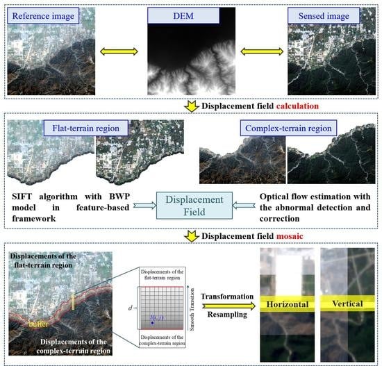
:While geometric registration has been studied in remote sensing community for many decades, successful cases are rare, which register images allowing for local inconsistency deformation caused by topographic relief. Toward this end, a region-by-region registration combining the feature-based and optical flow methods is proposed. The proposed framework establishes on the calculation of pixel-wise displacement and mosaic of displacement fields. Concretely, the initial displacement fields for a pair of images are calculated by the block-weighted projective model and Brox optical flow estimation, respectively in the flat- and complex-terrain regions. The abnormal displacements resulting from the sensitivity of optical flow in the land use or land cover changes, are adaptively detected and corrected by the weighted Taylor expansion. Subsequently, the displacement fields are mosaicked seamlessly for subsequent steps. Experimental results show that the proposed method outperforms comparative algorithms, achieving the highest registration accuracy qualitatively and quantitatively.
1. Introduction
The spatial position consistency of the same objects in multiple images guarantees the subsequent applications accuracy of remote sensing [1,2], medical imaging [3,4] and computer vision fields [5,6]. It is usually enforced by the means of geometric registration, which is a process of aligning different images of the same scene acquired at different times, viewing angles, and/or sensors [7].
In particular, quite a few algorithms have been proposed over the past decades for remote sensing images registration, broadly falling into two categories [8,9], i.e., the area-based methods and the feature-based methods. The area-based methods register images with their intensity information directly, whereas they are disabled to cope with large rotation and scale changes [10]. Consequently, more attention has been paid to feature-based methods [10,11,12,13,14,15,16]. The sensed image is aligned to the reference image by their significant geometrical features rather than intensity information, including feature extraction, feature matching, transformation model construction, coordinate transformation, and resampling [14]. Taking the feature point extraction as an example, the scale-invariant feature transform (SIFT) [17], the speeded-up robust feature (SURF) [18], and the extended SIFT or SURF [15,16] are well-known operators. The exhaustive search method [17] and the KD-tree matching algorithm are popular representatives of feature matching. The random sample consensus (RANSAC) [19] or maximum likelihood estimation sample consensus (MLESAC) [20] is applied to purify the matched features [21], namely outliers elimination. Successively, designing the geometric relationships for coordinate transformation, the global transformation model is the traditional and typical representation [9], which usually results in local misalignments for local and complicated deformations.
The local transformation model designs varied mapping functions for a whole image, including piecewise linear mapping function (PLM) [22], weighted mean (WM), multiquadric (MQ) [23], thin-plate spline (TPS) [24], and two-stage local registration model BWP-OIS [25]. The registration accuracy of the local model highly depends on the modeling type and is further determined by the distribution, number and position precision of feature points [23]. Nevertheless, the feature point extraction of the complex-terrain image is arduous due to the monotonous texture and degraded image quality. In addition, the pixel correspondences between images destroyed by varied geometric deformations could not be precisely acquired by current local models [26]. That is to say, it is difficult to achieve high-precision registration in the complex-terrain region under the feature-based framework although it performs well in most scenarios. To this end, a pixel-wise registration method should be taken into consideration.
Optical flow estimation is a pixel-wise algorithm firstly introduced by Horn and Schunch [27] in the field of computer vision for motion estimation. Afterwards, some modified models are proposed for high-precision motion estimation of video images [28,29]. As the geometric deformation of the corresponding pixels in multiple remote sensing images is similar to the object motions in successive frames, the optical flow algorithm was available for remote sensing images registration. However, its applications are rare in the remote sensing field. Only in recent years, the sparse optical flow algorithm is conducted for multi-modal remote sensing images registration on a single scenario, which does not need to process the abnormal displacements caused by land use or land cover (LULC) changes [26,30,31].
Due to the large field of view, a remote sensing image generally covers a large scene, containing the residential region, mountainous region, and agricultural region, etc. simultaneously. Different regions in the same scene involve locally varied geometric distortions with the topographic relief, for example, the complicated deformation in the complex-terrain region and locally consistent geometric distortion in the flat-terrain region. Moreover, LULC changes are frequent phenomena in multiple remote sensing images, which is an obstacle for pixel-wise registration algorithms to some extent. For the aforementioned two points, we propose a region-by-region registration combining feature-based and optical flow algorithms for remote sensing image, which is based on the mosaic of their individual displacement field. The main contributions of this paper include two aspects. One gives a novel region-by-region registration framework achieving highly precise registration of the whole scene considering the topographic relief. The other is to propose a correction approach for abnormal optical flow field caused by the LULC changes, integrating the adaptive detection and seamless correction by the weighted Taylor expansion.
The rest of this paper is organized as follows. The details of the proposed registration method are introduced in Section 2. The experimental results and verification from the visual and quantitative perspectives are provided in Section 3. Subsequently, the core parameter analysis is performed in Section 4. Finally, our conclusions are summarized in Section 5.
2. Methodology
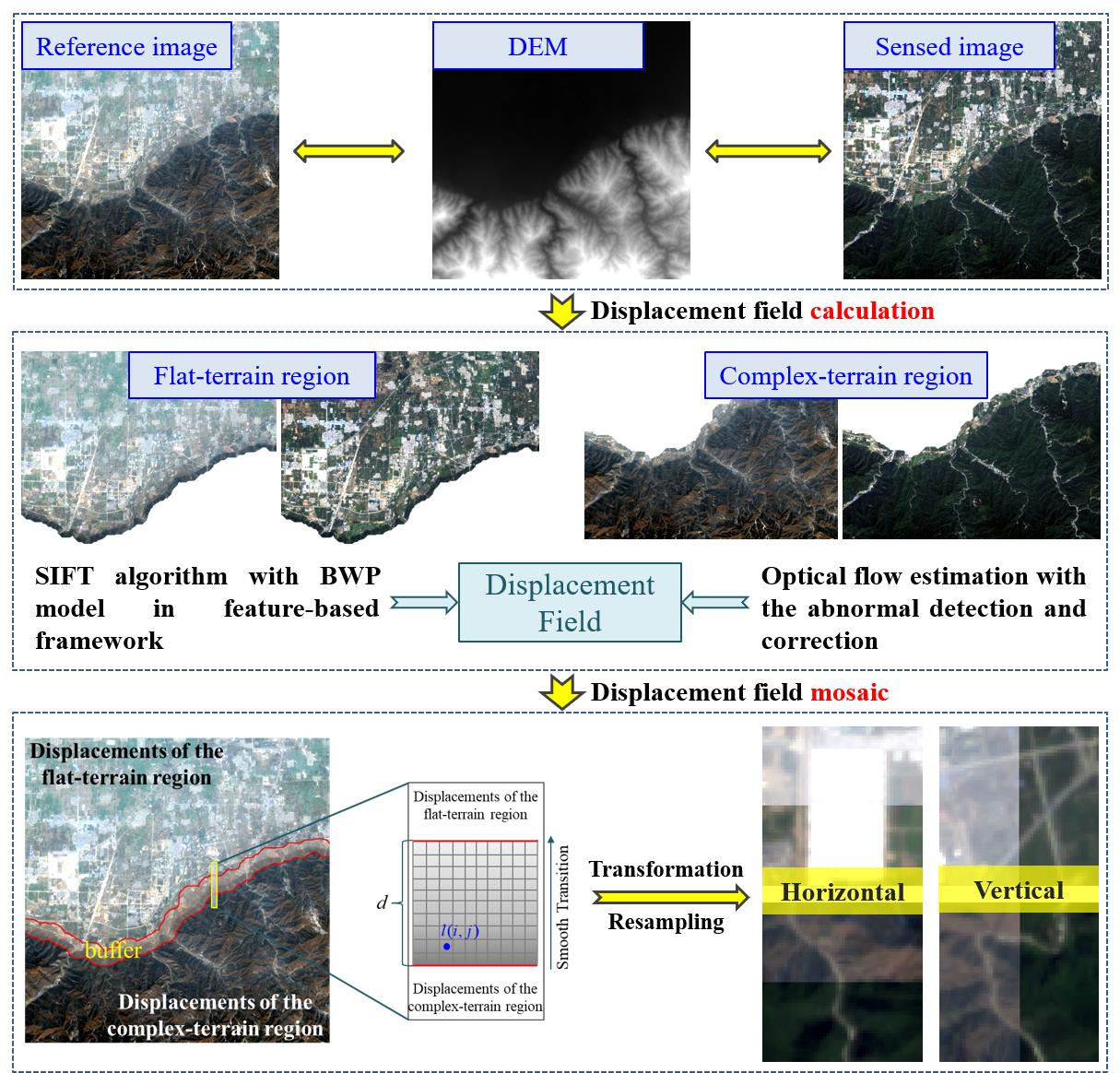
Allowing for the varied geometric distortions from the topographic relief in different regions of the remote sensing image, a novel region-by-region registration algorithm is proposed, as shown in Figure 1. Firstly, the initial pixel-wise displacement fields are calculated by the BWP model and the BOF estimation in the flat-terrain and complex-terrain regions, respectively. Secondly, the abnormal displacements correction is conducted by integrating the feature-based GP model for adaptive detection with the weighted Taylor expansion for thorough modification. Afterwards, the displacement fields of flat- and complex-terrain regions are mosaicked to generate a seamless one. Ultimately, the aligned image is obtained by the coordinate transformation and resampling.
2.1. Initial Displacements Calculation
As mentioned above, remote sensing images to be registered are divided into a series of flat- and complex-terrain parts in accordance with their topographic characteristics for initial displacement calculation. Since the elevation data is the typical representation of the terrain characteristics, among many sets of elevation data, considering the stability and wide availability, the digital elevation model (DEM) of the optimized shuttle radar topography mission (SRTM) was employed in our experiments. The local elevation difference (LED) indicating the terrain differences among the adjacent DEM cells in a specified window, is screened as the criterion of region division. Herein, LED is calculated by the elevation differences from the central cell to its eight neighbors.
where represents the elevation in the i-th local window and is the local terrain difference of the central pixel. is the terrain mask, and it equals one when is larger than the threshold , otherwise zero. is an integer ranging from five to eight, which is empirically set as seven in the experiment. However, there are inevitable fragmentary blobs, e.g., a small hole belonging to the complex-terrain region appears in the flat-terrain region. The hole-filling algorithm [32] and the morphological expansion approach [33,34] are utilized for terrain mask post-processing, where the expansion radius is set as ten. In this way, images are divided into different parts with two kinds of terrain characteristics. The displacement fields of the flat- and complex-terrain regions will be calculated by the feature-based BWP model and BOF estimation, respectively.
2.1.1. Displacements Calculation in the Flat-Terrain Region
In the flat-terrain region, the feature-based method is utilized to calculate the pixel-wise displacements between the reference and sensed images. The feature points are extracted by SIFT and matched by the nearest neighbor distance ratio (NNDR) algorithm for transformation model construction [17]. As one of the local models, BWP is employed to calculate the displacements [35] by dividing the image into blocks and designing block-wise geometric relationships. Generally, if the transformed point in the sensed image coincides with the original corresponding point in the reference image with the transformation model , it is rewritten as [14]. Linearizing the equation and the projective transformation model of a specified block is estimated as follows [25].
where is the number of the matched feature points. is the left part of the linearized and represents the stack of all . is the weight of the specified feature point calculated by the inverse distance weight (IDW) function, varying with blocks. For each block, with the transformation model , the pixel-wise displacement is calculated:
2.1.2. Displacements Estimation in the Complex-Terrain Region
As for the displacement field estimation in the complex-terrain region, the classical motion estimation method proposed by Brox et al. [36] is employed (namely BOF) and rewritten as follows:
where is the displacement field, and represents the coordinate in the reference image. and mean the intensity value in the specified location of the sensed and reference image, respectively. is the gradient. is modified minimization. and are the weights of gradient consistency and smoothness terms, respectively.
2.2. Abnormal Displacements Correction
However, BOF is sensitive to occlusions, which is similar to the LULC changes of remote sensing images, leading the abnormal displacements. These abnormal displacements will successively result in the changed content of the aligned image. Therefore, they should be corrected by the following algorithms.
2.2.1. Incorrect Displacements Detection
Generally, abnormal displacements appear in the region where the objects in the reference image could not be sought in the sensed image. In this situation, the displacements are discontinuous and mutational compared to their surroundings, with large or small magnitude as well as different directions. Since the feature-based global model obtains the continuous and stabilized displacement field even around the region of LULC changes, it is exactly used for detecting the abnormal displacements. By comparison with the displacements of the feature-based method, the abnormal displacements of BOF are adaptively detected by a given threshold. Concretely, the feature points are extracted by SIFT. The relationship between the reference and the sensed image assumes to be described by the GP model . Then the pixel-wise displacement is generated by Equation (5) and the mask for abnormal displacement is obtained in Equation (6).
where represents the displacement differences in and directions. and are the thresholds determined by the specified percentile of the ascending-order . It is hard to detect abnormal displacements identical to the LULC changes. To ensure the correction effect, the detected abnormal displacements are appropriately enlarged than the actual size of LULC changes with the thresholds. Our experiments verified that extra small-scale false abnormal displacements (in fact, they are normal displacements) will not reduce the final registration accuracy. According to our experimental experience, the available percentage range is [0.7, 0.9], which is set as 0.75 in the following experiments.
2.2.2. Incorrect Displacements Rectification
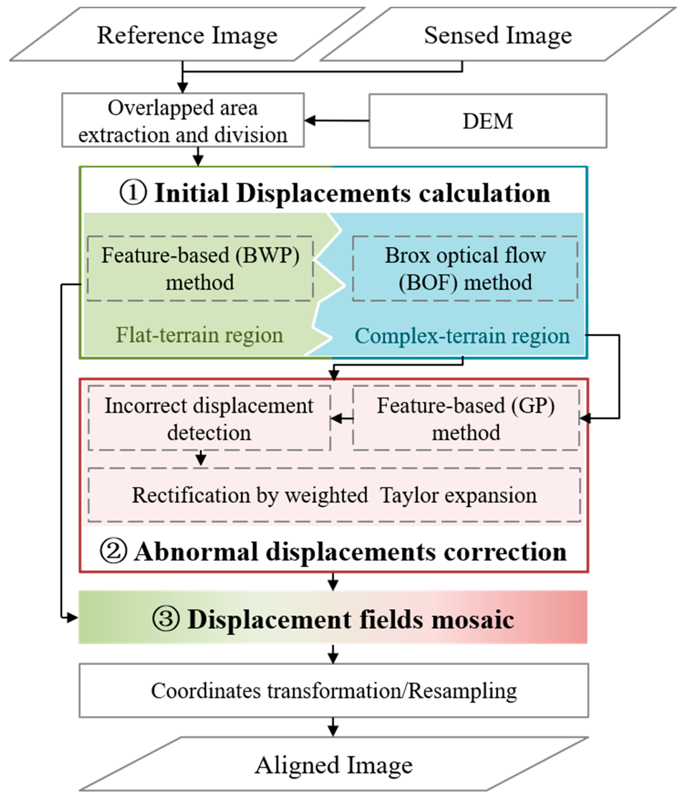
Guided by the mask from the detection result, the abnormal displacements will be corrected by the weighted first-order Taylor expansion. As illustrated in Figure 2, the abnormal displacements on the boundary are firstly recalculated, utilizing the neighboring accurate displacements specified with a yellow dotted rectangle. The boundary gradually propagates into the abnormal displacement region in white along the direction of arrows, until it is corrected completely.
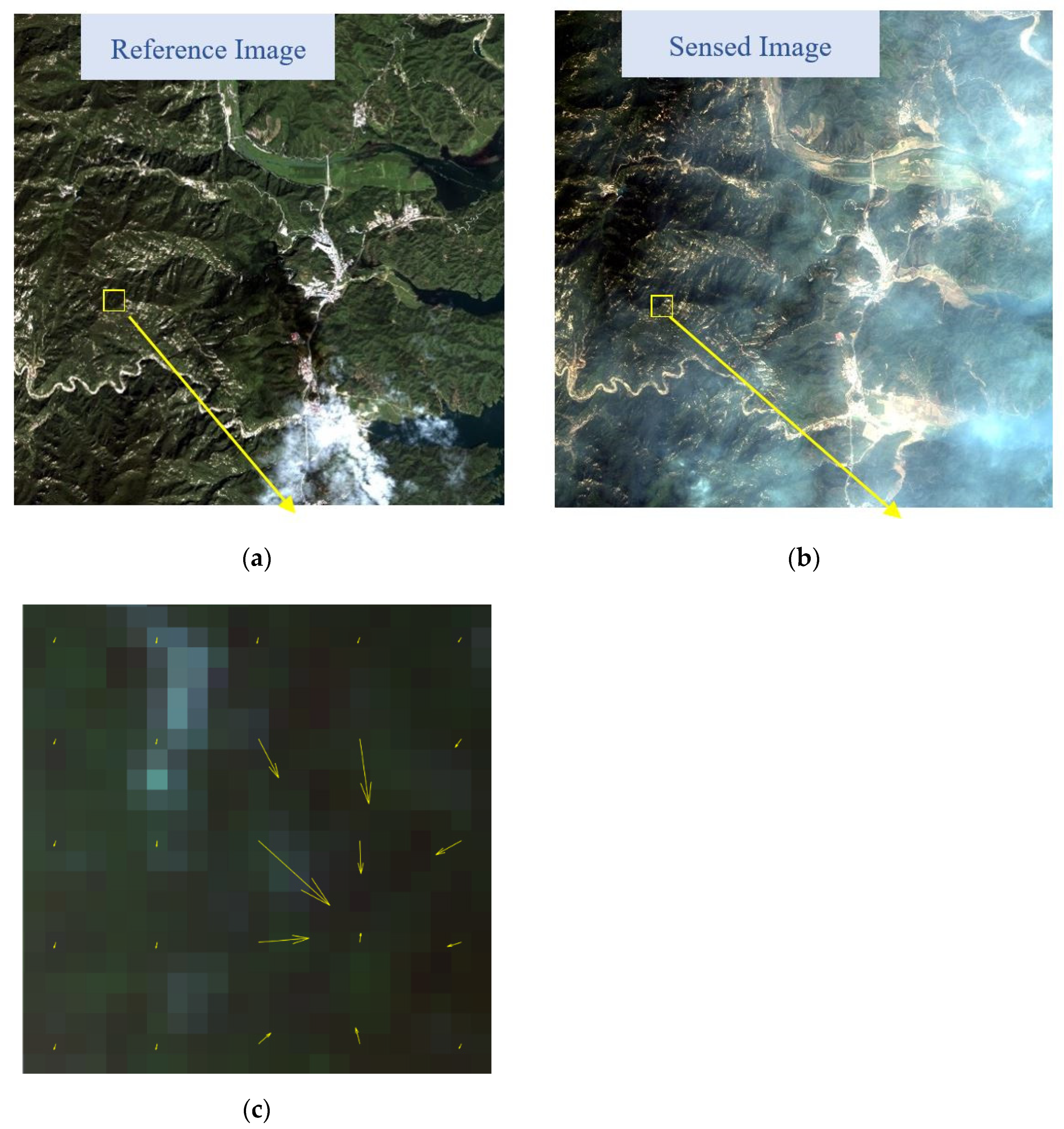
Concretely, supposing is the position of an abnormal displacement, it will be corrected with in its neighborhood . There is an assumption that the displacement variation is locally small in [37,38], as shown in Figure 3. As seen, taking part of the displacement field, owning 21 × 21 pixels, the displacement is displayed with yellow arrow every 5 pixels. Except the abnormal displacements in the lower right corner, the displacement variation is locally small in both magnitude and direction, which is consistent with the continuous law of remote sensing image. Under this circumstance, the displacement in (denoted as ) could be written by the first-order Taylor series expansion in Equation (8) [37,38].
where is the gradient of the displacement vector and contains x- and y-direction gradient. denotes the coordinate difference between pixels and . The abnormal displacement of (denoted as ) is recalculated by Equation (9).
where is a weighting function by the product of two essential factors. One is the geometric distance , and the other is the structural similarity . is calculated by IDW, which means that the closer to the pixel to be corrected, the greater the weight.
The neighboring pixels with similar structures from the same object possibly own a similar displacement. The image structure extracted by the phase congruency [13], is similar to the image gradient whereas it is insensitive to illumination and contrast changes. The LULC changes in the sensed image will lead to incorrect weight. Therefore, structural similarity is calculated in the reference image.
Equation (11) should not be calculated if the denominator is zero. represents the coordinate of the specified pixel. means the phase congruency in the reference image. Although the measure does not capture the exact structure similarity between and , the structural similarity between and on the reference image gives an approximation.
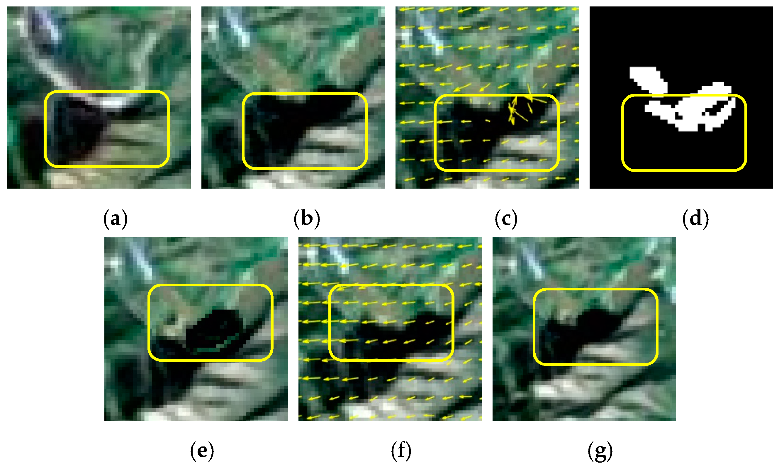
To summarize, with the geometric distance term , the effect from distant accurate displacement decreases. Additionally, the structure similarity approximates anisotropic propagation of neighboring accurate displacement. To avoid a jump between the corrected displacements and the original accurate displacements, the median filtering is conducted for the ultimate adjustment. An example of abnormal displacement detection and correction is shown in Figure 4. Figure 4a,b are the reference and sensed images. The LULC changes are marked with a yellow round rectangle. It leads to abnormal displacements estimation in Figure 4c, where the magnitude and direction of displacements are inconsistent with their neighborhood. The abnormal displacements further change the image content, comparing the region marked with a yellow round rectangle in Figure 4b,e. The abnormal displacements are detected and their corresponding mask is shown in Figure 4d. The white pixels represent the abnormal displacements and the black means the accurate ones. The abnormal displacements are corrected and shown in Figure 4f, where the corrected displacements are similar to the displacements in their surrounding region. Furthermore, the aligned image (see Figure 4g) is similar to the corresponding region in the sensed image in Figure 4b. Thus, the corrected BOF method is effective for abnormal displacement correction.
2.3. Displacement Fields Mosaic
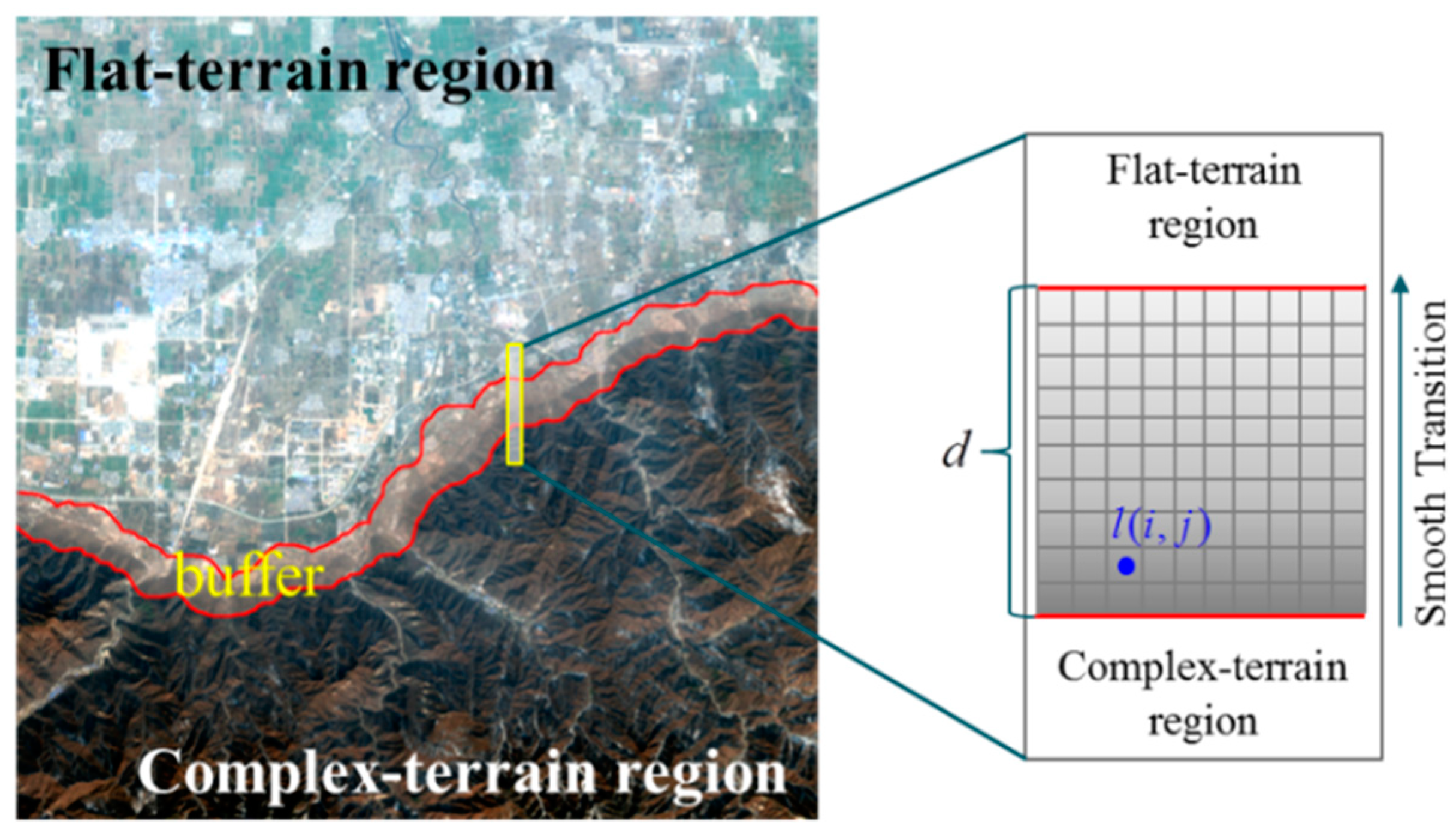
As mentioned previously, the proposed algorithm respectively calculates the displacements of flat-terrain and complex-terrain regions. To generate a displacement field for the entire image, the displacement fields from different regions should be mosaicked. Avoiding the jump at the edge of different displacement fields, for example, a buffer is constructed for two displacement fields, as shown in Figure 5, which is similar to image mosaic [39]. Outside the buffer, the displacements at the bottom and top come from the corrected BOF and feature-based BWP, respectively. Inside the buffer, each pixel’s displacement is a weighted combination of the two displacement fields. Without any loss of generality, we choose a simple weighted standard: distance. For example, as shown in Figure 5, for any pixel in the buffer, the distance is the buffer size from the bottom border to the top. The closer the pixel lies to the bottom of the buffer, the heavier the weight of the displacement from the complex-terrain region is, and the lighter the weight of the flat-terrain region displacement is; and vice versa.
Concretely, supposing is the final mosaicked displacement field, it is calculated as follows.
where and are the respective weights of displacement in the complex- and flat-terrain part in the buffer. is the displacement field from the complex-terrain region. represents the complex-terrain region and is the flat-terrain region. It is required that and . Therefore, the weight could also be designed according to IDW. Supposing that the distance of any pixel in the buffer to the border closer to the complex-terrain region is denoted as .
According to these principles, the displacement in the buffer area transits smoothly and a seamless displacement field is obtained. With the whole displacement field, the coordinates in the sensed image are directly transformed. After resampling, the aligned image is obtained.
3. Experiments and Evaluations
In this section, four representative pairs of remote sensing images in Table 1 were testified to evaluate the proposed algorithm qualitatively and quantitatively. Firstly, the results of the proposed method were visually compared with those of three local transformation models under the feature-based framework and the original optical flow estimation, i.e., PLM [22], TPS [24], BWP-OIS [25], and BOF [36]. PLM designs a series of local affine transformation models for each triangle constructed by the extracted feature points [22]. TPS estimates the geometrical relationship between the reference and sensed image by a systematic affine transformation model and a weighted radial basis function for considering local distortion [24]. BWP-OIS locally registers images in a two-step process by integrating the block-weighted projective transformation model and the outlier-insensitive model [25]. BOF registers the image by directly transforming the coordinates and resampling with pixel-wise displacements calculated under the brightness consistency and the gradient consistency [36]. Secondly, three assessment indicators were used for quantitative evaluation in Section 3.2, including root-mean-square error (RMSE), normal mutual information (NMI), and correlation coefficients (CC).
3.1. Visual Judgment
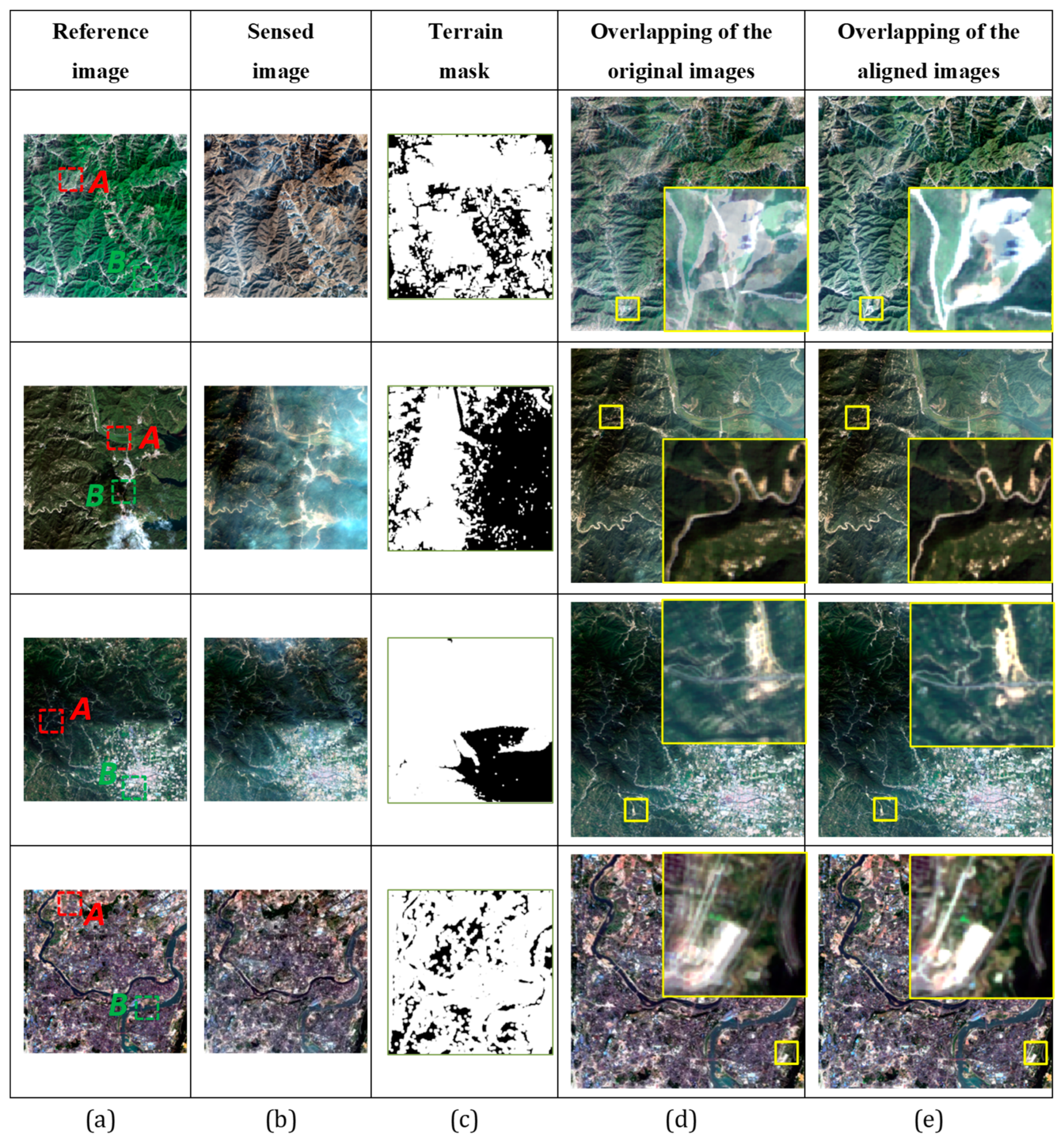
The registration results of the proposed algorithm are shown in Figure 6. As seen from the original images in Figure 6a,b, they show a large radiation difference (“test-I”), or are contaminated by uneven clouds (“test-II”), or include typical hybrid terrain region (“test-III”), or cover the complicated terrain (“test-IV”). The terrain mask is calculated by TR in Equation (1) and shown in Figure 6c. The white pixels represent the complex-terrain region and the black ones mean the flat-terrain region. They are approximately consistent with the visual observation and elevation data. Especially, since the test-IV images are located in Chongqing, China, which is known as the "mountain city", most of the image is in the complex-terrain region and they are white in the terrain mask. The overlapping results of the original images in Figure 6d show blurs and ghosts, which indicates that the geometrical deformation exists between reference and sensed images. By contrast, the overlapping results of aligned images by the proposed algorithm in Figure 6e are visually clear and distinctive. In other words, the experiments demonstrate the effectiveness of the proposed algorithm.
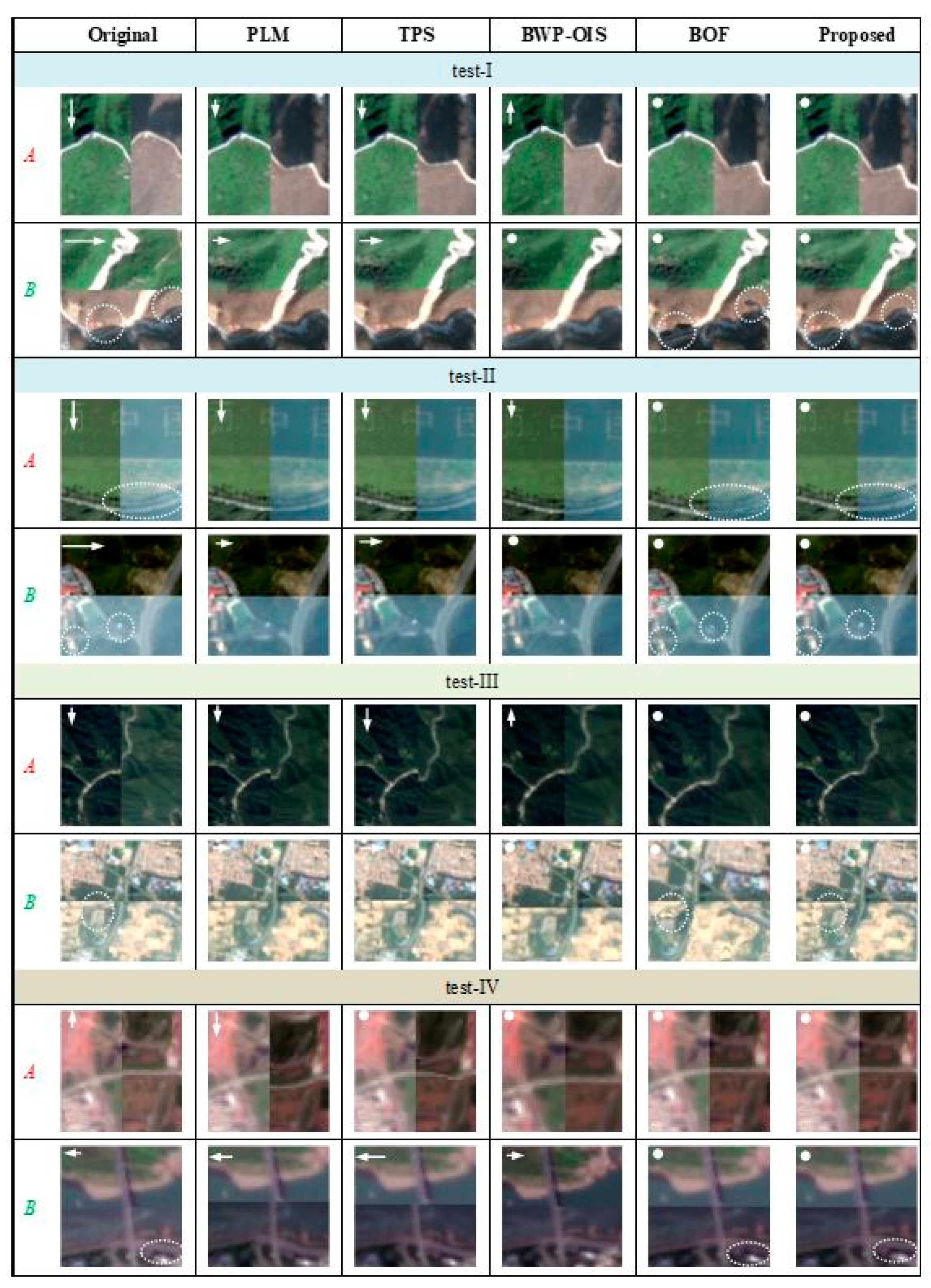
Successively, the comparison results of the proposed algorithm and other comparative methods are shown in Figure 7, which are the enlarged sub-regions of the red and green dotted-rectangle regions in Figure 6a for fine comparisons. The vertical alignment is labeled with red “A” and the horizontal alignment is marked with green “B”. The boundaries of the reference and aligned images are available to judge the registration accuracy. The white arrows and filled circles are auxiliary to indicate the displacements between the reference and aligned image. The arrows depict the direction of misalignment and their lengths are proportional to the amount of dislocation from the aligned image to the reference image. The white filled circles represent the well-registered results.
While focusing on the first comparison for “test-I” in Figure 7, row “A” shows the vertical registration of different methods. The “Original” broken linear features mean a large vertical deformation between the reference and sensed images. PLM and TPS eliminate the most of vertical deformation, but not completely. BWP-OIS results in overcompensation [25] to the sensed image so that the opposite misalignment of the linear features is introduced on the boundary. BOF and the proposed algorithm achieve highly accurate registration, where the linear features are continuous and smooth at the same position. For row “B”, though most of the horizontal displacements have been eliminated, the results of PLM and TPS still have dislocations. BWP-OIS, BOF, and the proposed algorithm register the sensed image well. However, the abnormal objects are introduced by BOF, which are not visible in the aligned image of the proposed method, marked with the white dotted ellipses. Therefore, the proposed algorithm gives high registration accuracy and guarantees the content against changes simultaneously.
The second comparison is for “test-II” in Figure 7. In Row “A”, the road at the bottom and the edge of the second Chinese character on the top are used to judge the registration result. The second Chinese character should be symmetrical, whereas its left and right parts are asymmetries due to the vertical dislocation. Although PLM aligns the road continuously and smoothly, the deformation of the second Chinese character is magnified. TPS could not align the sensed image well to the reference image. The Chinese character is aligned by BWP-OIS, but the road is not continuous. Fortunately, BOF and the proposed algorithm obtain the well-aligned outcomes for the road and the second Chinese character. However, the road on the result of BOF is changed. In “B” row, the road in the sensed image is shifted a lot to right by PLM and TPS. The proposed algorithm, BOF, and BWP-OIS provide the desired alignments. The only drawback is the content of the sensed image is altered by BOF. Therefore, PLM and TPS fail to align the sensed image to the reference image spatially. BWP-OIS gives desirable registration in the horizontal direction but not in the vertical direction. BOF generates accurate alignments accompanied by abnormal changes marked with white dotted ellipses. The proposed algorithm outperforms others in alignment with accuracy or content fidelity.
The selected regions in “test-III” and “test-IV” in Figure 6 further verify the proposed algorithm, as shown in Figure 7. For “test-III” in Figure 7, a similar phenomenon is observed, where the proposed algorithm outperforms others both in the vertical and horizontal directions. The phenomenon of the content change introduced by BOF is removed by the proposed algorithm. For “test-IV” in Figure 7, the other three algorithms excluding PLM provide the well-aligned outcomes in “A” row. In “B” row (test-IV), PLM and TPS widen the dislocation, and BWP-OIS introduces the opposite misalignment of the bridge. BOF and the proposed algorithm completely eliminate the deformation and the bridge is connected smoothly and continuously. However, BOF changes the content (labeled by a white dotted ellipse), and the proposed algorithm keeps the content of the sensed image well. In conclusion, the proposed algorithm visually outperforms other algorithms in all experiments. To further evaluate the proposed algorithm, the quantitative evaluation is conducted.
3.2. Quantitative Evaluation
The quantitative evaluation with three indictors was further used for verifying the visual judgment. On one hand, RMSE depicts the spatial registration accuracy. On the other hand, NMI and CC judge the similarity between the aligned image and the reference image according to their corresponding pixel values.
The RMSE focuses on evaluating the registration result by calculating the average distance of the corresponding points in the reference and aligned image. As most literature did, some distinct feature points from the corresponding reference and aligned images were extracted manually to calculate their RMSE [7,40]. RMSE of the comparative algorithms is listed in Table 2. The feature points for evaluation are extracted manually and the number is listed in brackets. “Original” means the RMSE of the reference and sensed image before registration. All the algorithms relieve the geometric distortion of the reference and sensed image as shown in Table 2. TPS gives the largest RMSE among all registration algorithms. BWP-OIS performs better than PLM in the last three experiments. The smallest RMSE is obtained by the proposed algorithm and the suboptimal performance is given by BOF. Since there are some abnormal objects and pseudo traces in the aligned image of BOF, these anomalies change the shape or the original track of linear features in the aligned image, causing lower registration accuracy. The proposed algorithm performs better than the three feature-based algorithms, which means that it is more favorable for registering complex-terrain regions. Furthermore, RMSE of the proposed algorithm is smaller than that of BOF, indicating that the feature-based method owns the similar registration accuracy without being affected by the LULC changes in the flat-terrain region, and the proposed algorithm copes with the LULC changes in the complex-terrain region well.
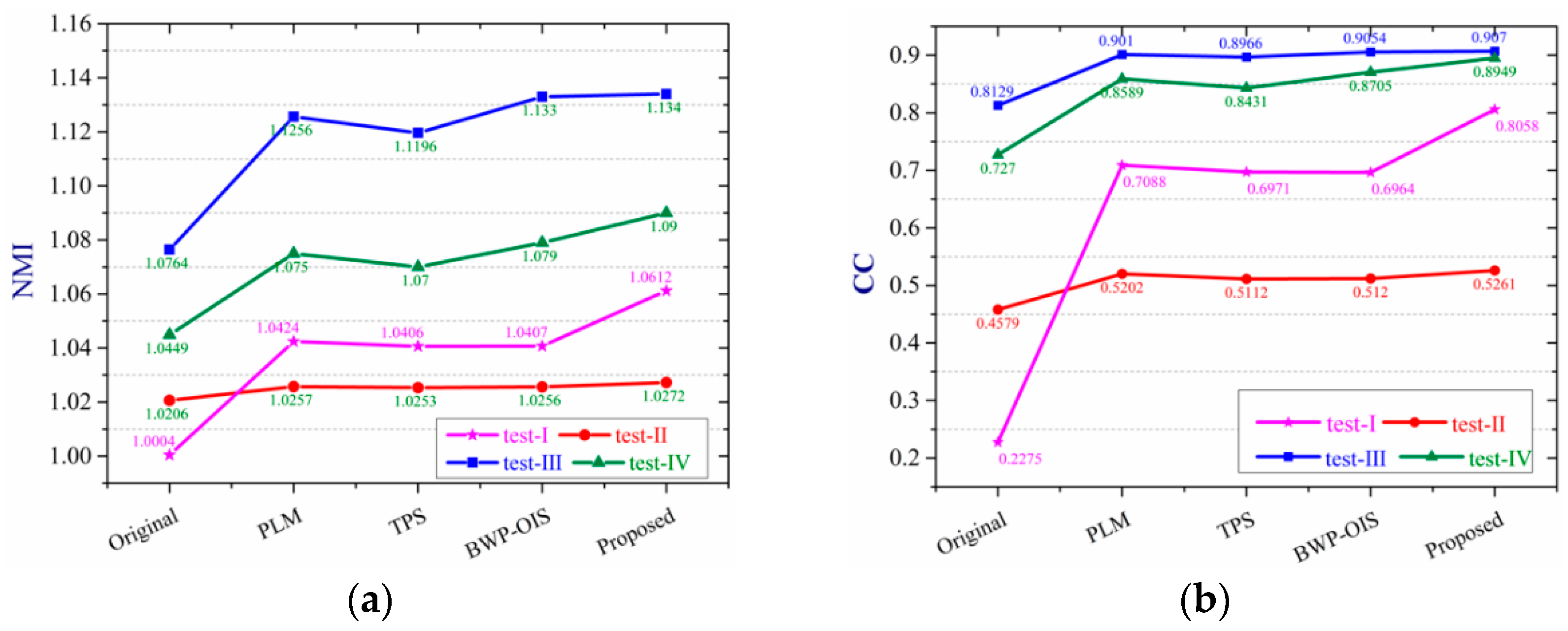
To further evaluate the performance of the proposed method, we extract the complex-terrain region of the aligned image and the corresponding part in the reference image. The extracted ones of the above experiments are conducted to calculate the NMI and CC shown in Figure 8a,b. NMI and CC are the similarity criteria, usually employing as the iteration termination condition in the area-based registration algorithm. The NMI index measures the statistical correlation of images, which is defined as follows:
where and are the entropy of images and , respectively. is the joint entropy of two images. Larger NMI correspond to a greater similarity between two images. The CC value of images and is calculated as:
where denotes covariance between two images. and are the standard deviations of two images, respectively. Since CC could range from −1 to 1, 1 indicates perfect correlation.
As shown, the proposed method achieves the largest NMI and CC in all the experiments. The registration accuracy of PLM is close to that of BWP-OIS whereas the latter is slightly superior in “test-III” and “test-IV” in Figure 8. The local mapping functions of PLM are constructed by feature points, so its accuracy is limited by the precision of the feature points extraction. On that account, BWP-OIS alleviates the situation by designing the transformation functions with all feature points in different weights. Therefore, BWP-OIS performs better than PLM in most instances. Additionally, TPS gets the worst registration accuracy in four experiments, which is suitable for images with dense and uniformly distributed feature points [23]. It is difficult to extract feature points in the complex-terrain region, especially points with uniform distribution. In addition, the registration accuracy of BOF is comparable to the proposed method in the complex-terrain regions when evaluating with NMI and CC, which is similar to the RMSE result. In addition, it is worth noting that there is a big jump on test-I. It is because there is a large deformation between the reference and sensed images, resulting in the smaller NMI and CC compared with those of the registration results. On the one hand, not only the local region rounded with yellow rectangles of test-I in Figure 5 presents an obvious geometric dislocation; but the RMSE of the test-I original images in Table 2 is larger than those of other experiments. Hence, there is a big jump in Figure 8 of NMI and CC values on test-I. The proposed method automatically registers images, including image division according to the terrain characteristics, alignment of flat-terrain region with feature-based algorithm, the pixel-wise displacement calculation of complex-terrain region with improved optical flow estimation. The thresholds in these steps are determined with the experience of a large number of experiments. The evaluation demonstrates that the proposed method performs well on the mixed-terrain region compared with the conventional feature-based methods and the original optical flow algorithm. To a certain extent, it also shows that the scheme of region-by-region registration is feasible.
4. Discussions
The previous section validated the registration result of the proposed method. This section focuses on core parameter analysis. The main parameter is the LED threshold for the terrain division, determining the algorithm utilized to register the local region of images and further influencing the final registration accuracy.
for terrain division determines that a pixel should be divided into the complex terrain region or flat-terrain region, which further influences the overall registration accuracy. To reveal the relationship, a series of experiments were conducted with different thresholds. Without loss of generality, the aforementioned experimental data in Figure 6 is employed, with the threshold varied from five to thirteen. The quantitative evaluation results of the final registration with varied thresholds are shown in Table 3, with the evaluation indicators of NMI and CC.
For the four groups of experiments, with the increase in the threshold, the two indicators are at first small fluctuations, or even stable, and then decrease, showing the relatively simple relationship. However, focusing on the quantitative evaluation of “test-III”, the largest NMI is obtained when the LED threshold is set as eight whereas the best CC is generated while equals six. Except for the third experiment, they share the same phenomenon, in that the optimal registration results are obtained while the LED threshold is set as seven. When the threshold is larger than seven, more pixels are put into the flat-terrain region whereas the complex terrain is in practice, weakening the registration accuracy. However, this does not mean that the smaller the threshold is, the higher the registration accuracy will be, such as the third and fourth groups of the experiments. However, when the available range of LED threshold is five to eight, the indicators do not show an obvious difference, where the largest numerical difference is 0.0008. Under this circumstance, the difference between the different registration results could not be caught by the eyes. After the comprehensive consideration, the LED threshold was determined to be seven in the experiments.
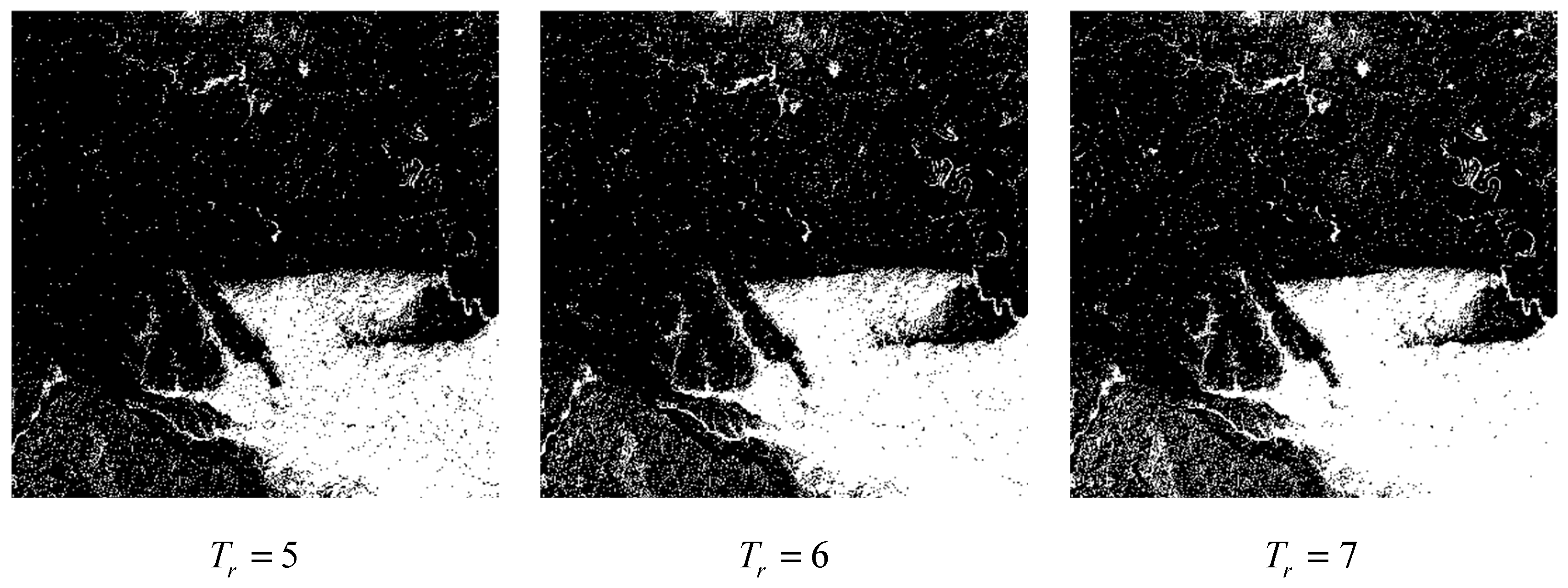
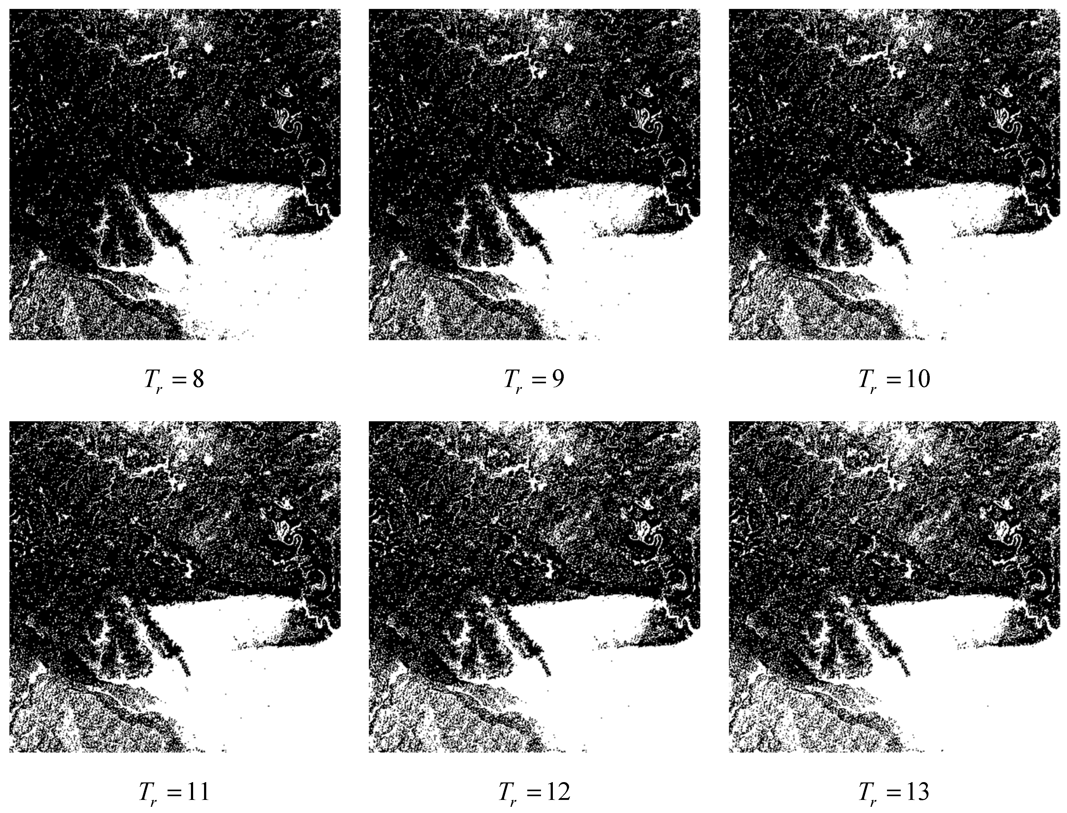
For conveniently applying this technique, taking test-III as an example, the terrain masks generated by different thresholds are listed in Figure 9. The intention is to divide the image to be registered into multiple local regions with flat- and complex-terrain characteristics. That is to say, the heterogeneous features distributed in a topographic block are not put into this block as far as possible. Therefore, the hole-filling algorithm and the morphological expansion approach are utilized, as described in Section 2.1. Before the post-processing of the terrain mask, the generated mask should provide an ideal foundation. The threshold of LED for terrain division is set with the visual observation and the quantitative evaluation of registration result. In Figure 9, the black indicates the complex-terrain region, and white means the flat-terrain region. When the threshold is 5, there are heterogeneous and small blobs both in the complex- and flat-terrain regions. While the threshold is 7, there are relatively few heterogeneous blobs in the flat-terrain region (denoted in white), and more white blobs in the complex-terrain region, compared with the first two masks. When compared with the last six masks, the terrain division is relatively regular, namely most flat-terrain pixels are in the white region and complex-terrain blobs are in black. The conclusion is similar to Table 3. Not only test-III but three other experiments also give a similar conclusion, which is not shown here. Therefore, after quantitative comparison and qualitative observation of a large number of experiments, we provide the available range of the threshold in Section 2.1 and the best recommended threshold is seven.
5. Conclusions
In this paper, we proposed a region-by-region registration combining feature-based and optical flow methods for remote sensing images. The proposed method innovatively makes use of the geometric deformation characteristic varied with regions caused by the topographic relief, registering flat- and complex-terrain regions, respectively. Owing to the pixel-wise displacement estimation of dense optical flow algorithm, the registration accuracy in complex-terrain region is reinforced. Moreover, the adaptive detection and weighted Taylor expansion enforced makes up for the defect of the abnormal displacements in the LULC changed region, which is sensitive for dense optical flow estimation. In other words, the feature-based method, dense optical flow estimation, adaptive detection technique, and weighted Taylor expansion are all employed for high-precision pixel-wise displacements, further for accurate registration. The accuracy of the complex-terrain region determines the whole registration precision of images covering the mixed terrain, which has attracted much attention in the proposed framework, and is realized by improving the optical flow algorithm. As confirmed in the experiments, the proposed approach outperforms the conventional feature-based methods and the original optical flow algorithm, not only qualitatively, but also quantitatively, from the aspects of visual observation, NMI, CC and RMSE.
However, the proposed method is just an interesting first trial of mixed-terrain images registration. The result is preliminary, and there is still room for improvement. For instance, when the experiments are conducted on Matlab2018a settled on computer with an Intel (R) Xeon (R) CPU E5-2650 v2 2.6GHz, the runtime of our experiments is 295.237s, 294.044s, 373.050s, and 143.808s respectively. It is time-consuming to register images by the proposed algorithm, which exceeds the expected time of image registration in the pre-processing stage, even real-time processing. Therefore, the time efficiency needs to be improved with parallel processing on the C++ platform, particularly for the complex-terrain region alignment. Additionally, when registering two degraded images with optical flow algorithm in the complex-terrain region, both images are simultaneously contaminated at the same location and abnormal displacements could not be restored as the weight from phase congruency for Taylor expansion calculating abnormally, which further changes the aligned image content compared with sensed image. Moreover, more mixed-terrain images from other sensors should be further tested in experiments for our proposed method. These issues will be addressed in our future work.
Author Contributions
Conceptualization, R.F., X.L. and H.S.; methodology, R.F.; validation, R.F. and X.L.; formal analysis, R.F.; investigation, R.F. and X.L.; resources, H.S. and Q.D.; data curation, R.F.; writing—original draft preparation, R.F.; writing—review and editing, R.F., X.L. and H.S.; supervision, H.S. and Q.D.; project administration, H.S. and X.L.; funding acquisition, X.L. and H.S. All authors have read and agreed to the published version of the manuscript.
Funding
This research was funded by the National Natural Science Foundation of China (NSFC), grant number 41701394, 61671334 and 41901357; the Open Research Fund Program of the Key Laboratory of Digital Mapping and Land Information Application Engineering, the Ministry of Natural Resources, grant number ZRZYBWD201903, and the Fundamental Research Funds for the Central Universities, grant number GK202103143.
Institutional Review Board Statement
Not applicable.
Informed Consent Statement
Not applicable.
Data Availability Statement
Not applicable.
Acknowledgments
This article was completed during the first author’s doctoral study at Wuhan University, sorted and written in Shaanxi Normal University after graduation. Therefore, special thanks are given to the co-authors and others who helped with this article. In addition, thanks editor and assistant editor of Remote Sensing, as well as four anonymous reviewers for their advices and good idea to strength our manuscript.
Conflicts of Interest
The authors declare no conflict of interest.
References
- Ballesteros, R.; Ortega, J.; Hernandez, D.; del Campo, A.; Moreno, M. Combined use of agro-climatic and very high-resolution remote sensing information for crop monitoring. Int. J. Appl. Earth Obs. Geoinf. 2018, 72, 66–75. [Google Scholar] [CrossRef]
- Raza, S.-E.-A.; Sanchez, V.; Prince, G.; Clarkson, J.P.; Rajpoot, N.M. Registration of thermal and visible light images of diseased plants using silhouette extraction in the wavelet domain. Pattern Recognit. 2015, 48, 2119–2128. [Google Scholar] [CrossRef]
- So, R.W.; Chung, A.C. A novel learning-based dissimilarity metric for rigid and non-rigid medical image registration by using Bhattacharyya Distances. Pattern Recognit. 2017, 62, 161–174. [Google Scholar] [CrossRef]
- So, R.W.; Tang, T.W.; Chung, A.C. Non-rigid image registration of brain magnetic resonance images using graph-cuts. Pattern Recognit. 2011, 44, 2450–2467. [Google Scholar] [CrossRef]
- Hao, Y.; Li, J.; Wang, N.; Gao, X. Modality adversarial neural network for visible-thermal person re-identification. Pattern Recognit. 2020, 107, 107533. [Google Scholar] [CrossRef]
- Zhang, Y.; Shi, L.; Wu, Y.; Cheng, K.; Cheng, J.; Lu, H. Gesture recognition based on deep deformable 3D convolutional neural networks. Pattern Recognit. 2020, 107, 107416. [Google Scholar] [CrossRef]
- Wong, A.; Clausi, D.A. ARRSI: Automatic Registration of Remote-Sensing Images. IEEE Trans. Geosci. Remote Sens. 2007, 45, 1483–1493. [Google Scholar] [CrossRef]
- Ding, L.; Goshtasby, A.; Satter, M. Volume image registration by template matching. Image Vis. Comput. 2001, 19, 821–832. [Google Scholar] [CrossRef]
- Arce-Santana, E.R.; Alba, A. Image registration using Markov random coefficient and geometric transformation fields. Pattern Recognit. 2009, 42, 1660–1671. [Google Scholar] [CrossRef] [Green Version]
- Wu, Y.; Ma, W.; Su, Q.; Liu, S.; Ge, Y. Remote sensing image registration based on local structural information and global constraint. J. Appl. Remote Sens. 2019, 13, 1. [Google Scholar] [CrossRef]
- Chen, S.; Li, X.; Zhao, L.; Yang, H. Medium-low resolution multisource remote sensing image registration based on SIFT and robust regional mutual information. Int. J. Remote Sens. 2018, 39, 3215–3242. [Google Scholar] [CrossRef]
- Duan, Y.; Huang, X.; Xiong, J.; Zhang, Y.; Wang, B. A combined image matching method for Chinese optical satellite imagery. Int. J. Digit. Earth 2016, 9, 851–872. [Google Scholar] [CrossRef]
- Ye, Y.; Shan, J.; Bruzzone, L.; Shen, L. Robust Registration of Multimodal Remote Sensing Images Based on Structural Similarity. IEEE Trans. Geosci. Remote. Sens. 2017, 55, 2941–2958. [Google Scholar] [CrossRef]
- Zitová, B.; Flusser, J. Image registration methods: A survey. Image Vis. Comput. 2003, 21, 977–1000. [Google Scholar] [CrossRef] [Green Version]
- Chang, H.-H.; Wu, G.-L.; Chiang, M.-H. Remote Sensing Image Registration Based on Modified SIFT and Feature Slope Grouping. IEEE Geosci. Remote Sens. Lett. 2019, 16, 1363–1367. [Google Scholar] [CrossRef]
- Sedaghat, A.; Mohammadi, N. High-resolution image registration based on improved SURF detector and localized GTM. Int. J. Remote Sens. 2018, 40, 2576–2601. [Google Scholar] [CrossRef]
- Lowe, D.G. Distinctive Image Features from Scale-Invariant Keypoints. Int. J. Comput. Vis. 2004, 60, 91–110. [Google Scholar] [CrossRef]
- Bay, H.; Tuytelaars, T.; Van Gool, L. SURF: Speeded Up Robust Features. Lect. Notes Comput. Sci. 2006, 110, 404–417. [Google Scholar]
- Fischler, M.A.; Bolles, R.C. Random sample consensus: A paradigm for model fitting with applications to image analysis and automated cartography. Commun. ACM 1981, 24, 381–395. [Google Scholar] [CrossRef]
- Wang, Y.; Shen, J.; Liao, W.; Zhou, L. Automatic fundus images mosaic based on SIFT feature. In Proceedings of the 23rd International Congress on Image and Signal Processing, Yantai, China, 16–18 October 2010; pp. 2747–2751. [Google Scholar]
- Song, Z.; Zhou, S.; Guan, J. A Novel Image Registration Algorithm for Remote Sensing Under Affine Transformation. IEEE Trans. Geosci. Remote Sens. 2013, 52, 4895–4912. [Google Scholar] [CrossRef]
- Goshtasby, A. Piecewise linear mapping functions for image registration. Pattern Recognit. 1986, 19, 459–466. [Google Scholar] [CrossRef]
- Zagorchev, L.; Goshtasby, A. A comparative study of transformation functions for nonrigid image registration. IEEE Trans. Image Process. 2006, 15, 529–538. [Google Scholar] [CrossRef] [PubMed]
- Goshtasby, A. Registration of images with geometric distortions. IEEE Trans. Geosci. Remote Sens. 1988, 26, 60–64. [Google Scholar] [CrossRef]
- Feng, R.; Du, Q.; Li, X.; Shen, H. Robust registration for remote sensing images by combining and localizing feature- and area-based methods. ISPRS J. Photogramm. Remote Sens. 2019, 151, 15–26. [Google Scholar] [CrossRef]
- Brigot, G.; Colin-Koeniguer, E.; Plyer, A.; Janez, F. Adaptation and Evaluation of an Optical Flow Method Applied to Coregistration of Forest Remote Sensing Images. IEEE J. Sel. Top. Appl. Earth Obs. Remote Sens. 2016, 9, 2923–2939. [Google Scholar] [CrossRef] [Green Version]
- Horn, B.K.P.; Schunck, B.G. Determining optical flow. Artif. Intell. 1981, 17, 185–203. [Google Scholar] [CrossRef] [Green Version]
- Liu, C.; Yuen, J.; Torralba, A. SIFT Flow: Dense Correspondence across Scenes and Its Applications. IEEE Trans. Pattern Anal. Mach. Intell. 2011, 33, 978–994. [Google Scholar] [CrossRef] [Green Version]
- Lin, K.; Jiang, N.; Liu, S.; Cheong, L.-F.; Do, M.; Lu, J. Direct photometric alignment by mesh deformation. In Proceedings of the IEEE Conference on Computer Vision and Pattern Recognition (CVPR), Honolulu, HI, USA, 21–26 July 2017; pp. 2405–2413. [Google Scholar]
- Xiang, Y.; Wang, F.; Wan, L.; Jiao, N.; You, H. OS-Flow: A Robust Algorithm for Dense Optical and SAR Image Registration. IEEE Trans. Geosci. Remote Sens. 2019, 57, 6335–6354. [Google Scholar] [CrossRef]
- Plyer, A.; Colin-Koeniguer, E.; Weissgerber, F. A New Coregistration Algorithm for Recent Applications on Urban SAR Images. IEEE Geosci. Remote Sens. Lett. 2015, 12, 2198–2202. [Google Scholar] [CrossRef]
- Soille, P. Morphological Image Analysis: Principles and Applications; Springer Science & Business Media: Berlin/Heidelberg, Germany, 2013. [Google Scholar]
- van den Boomgaard, R.; van Balen, R. Methods for fast morphological image transforms using bitmapped binary images. CVGIP Graph. Models Image Process. 1992, 54, 252–258. [Google Scholar] [CrossRef]
- Blanchet, G.; Charbit, M. Digital Signal and Image Processing Using MATLAB; Wiley Online Library: Hoboken, NJ, USA, 2006; Volume 4. [Google Scholar]
- Feng, R.; Li, X.; Zou, W.; Shen, H. Registration of multitemporal GF-1 remote sensing images with weighting perspective transformation model. In Proceedings of the IEEE International Conference on Image Processing (ICIP), Beijing, China, 17–20 September 2017; pp. 2264–2268. [Google Scholar]
- Brox, T.; Bruhn, A.; Papenberg, N.; Weickert, J. High Accuracy Optical Flow Estimation Based on a Theory for Warping. In Proceedings of the European Conference on Computer Vision (ECCV), Prague, Czech Republic, 11–14 May 2004; pp. 25–36. [Google Scholar]
- Matsushita, Y.; Ofek, E.; Weina, G.; Xiaoou, T.; Heung-Yeung, S. Full-frame video stabilization with motion inpainting. IEEE Trans. Pattern Anal. Mach. Intell. 2006, 28, 1150–1163. [Google Scholar] [CrossRef] [PubMed]
- Telea, A. An Image Inpainting Technique Based on the Fast Marching Method. J. Graph. Tools 2004, 9, 23–34. [Google Scholar] [CrossRef]
- Li, X.; Feng, R.; Guan, X.; Shen, H.; Zhang, L. Remote Sensing Image Mosaicking: Achievements and Challenges. IEEE Geosci. Remote Sens. Mag. 2019, 7, 8–22. [Google Scholar] [CrossRef]
- Han, Y.; Bovolo, F.; Bruzzone, L. An Approach to Fine Coregistration Between Very High Resolution Multispectral Images Based on Registration Noise Distribution. IEEE Trans. Geosci. Remote Sens. 2015, 53, 6650–6662. [Google Scholar] [CrossRef]
Figure 1.
The flow-chart of the processed algorithm.

Figure 2.
Abnormal displacement correction.

Figure 3.
Displacement field of the local region. (a) Reference image, (b) sensed image, (c) the displacement field of corresponding pixels in the yellow rectangle.
Figure 3.
Displacement field of the local region. (a) Reference image, (b) sensed image, (c) the displacement field of corresponding pixels in the yellow rectangle.

Figure 4.
The abnormal displacements correction. (a) Reference image, (b) sensed image, (c) the displacement field by Equation (6), (d) the mask for abnormal displacements, (e) the BOF aligned image, (f) the corrected displacements, (g) the aligned image after abnormal displacements correction.
Figure 4.
The abnormal displacements correction. (a) Reference image, (b) sensed image, (c) the displacement field by Equation (6), (d) the mask for abnormal displacements, (e) the BOF aligned image, (f) the corrected displacements, (g) the aligned image after abnormal displacements correction.

Figure 5.
Displacement field mosaic of flat-terrain and complex-terrain region.

Figure 6.
The registration results of the proposed method. From top to the bottom they correspond to test-I, test-II, test-III, and test-IV, respectively. (a) Reference image, (b) sensed image, (c) terrain mask (white means the complex-terrain region, otherwise are flat-terrain regions) the overlapping result of reference and (d) the sensed image, (e) the aligned image.

Figure 7.
Zoom-in results of red and green dotted-rectangle regions in Figure 6.
Figure 7.
Zoom-in results of red and green dotted-rectangle regions in Figure 6.

Figure 8.
(a) NMI and (b) CC of the aligned results from the compared methods.

Figure 9.
The terrain mask of test-III with different thresholds (Note: black represents the complex-terrain region and white means the flat-terrain region).
Figure 9.
The terrain mask of test-III with different thresholds (Note: black represents the complex-terrain region and white means the flat-terrain region).


Table 1.
Experimental data.
| Tab | Res. | Time | Sensor | Characteristics (All Located in China) |
|---|---|---|---|---|
| test-I | 4 m | 2016.05.06 | GF2_PMS2 | Near Jinan, a mixed region. |
| 2016.02.07 | ||||
| test-II | 4 m | 2016.08.27 | GF2_PMS2 | Northeast of Beijing, mixed terrain with clouds. |
| 2016.06.09 | ||||
| test-III | 16 m | 2017.08.10 | GF1_WFV1 | Northwestern of Zhengzhou, mixed region. |
| 2017.09.20 | ||||
| test-IV | 16 m | 2018.04.18 | GF1_WFV1 | The urban area of Chongqing, most are large topographic relief. |
| 2018.05.13 |
Table 2.
RMSE (↓) of different algorithms in the experiments (by pixels).
| Experiment | Original | PLM | TPS | BWP-OIS | BOF | Proposed |
|---|---|---|---|---|---|---|
| test-I (20) | 41.10 | 4.21 | 5.14 | 4.59 | 0.61 | 0.43 |
| test-II (20) | 3.14 | 1.12 | 1.23 | 1.02 | 0.62 | 0.40 |
| test-III (20) | 3.54 | 0.62 | 0.98 | 0.41 | 0.35 | 0.26 |
| test-IV (20) | 2.69 | 0.86 | 1.47 | 0.74 | 0.29 | 0.28 |
Table 3.
Quantitative evaluation of ultimate registration with different .
| Image | Indicator | 5 | 6 | 7 | 8 | 9 | 10 | 11 | 12 | 13 |
|---|---|---|---|---|---|---|---|---|---|---|
| test-I | NMI | 1.0612 | 1.0612 | 1.0612 | 1.0599 | 1.0587 | 1.0570 | 1.0529 | 1.0492 | 1.0465 |
| CC | 0.8058 | 0.8057 | 0.8058 | 0.7992 | 0.7919 | 0.7831 | 0.7592 | 0.7388 | 0.7227 | |
| test-II | NMI | 1.0272 | 1.0271 | 1.0272 | 1.0272 | 1.0271 | 1.0269 | 1.0268 | 1.0266 | 1.0265 |
| CC | 0.5256 | 0.5249 | 0.5261 | 0.5259 | 0.5250 | 0.5238 | 0.5227 | 0.5216 | 0.5203 | |
| test-III | NMI | 1.1342 | 1.1341 | 1.1340 | 1.1347 | 1.1347 | 1.1346 | 1.1345 | 1.1346 | 1.1346 |
| CC | 0.9071 | 0.9071 | 0.9070 | 0.9064 | 0.9064 | 0.9063 | 0.9062 | 0.9063 | 0.9063 | |
| test-IV | NMI | 1.0900 | 1.0900 | 1.0900 | 1.0900 | 1.0897 | 1.0895 | 1.0892 | 1.0889 | 1.0884 |
| CC | 0.8948 | 0.8948 | 0.8949 | 0.8948 | 0.8943 | 0.8939 | 0.8933 | 0.8925 | 0.8915 |
Publisher’s Note: MDPI stays neutral with regard to jurisdictional claims in published maps and institutional affiliations. |
© 2021 by the authors. Licensee MDPI, Basel, Switzerland. This article is an open access article distributed under the terms and conditions of the Creative Commons Attribution (CC BY) license (https://creativecommons.org/licenses/by/4.0/).
Share and Cite
MDPI and ACS Style
Feng, R.; Du, Q.; Shen, H.; Li, X. Region-by-Region Registration Combining Feature-Based and Optical Flow Methods for Remote Sensing Images. Remote Sens. 2021, 13, 1475. https://0-doi-org.brum.beds.ac.uk/10.3390/rs13081475
AMA Style
Feng R, Du Q, Shen H, Li X. Region-by-Region Registration Combining Feature-Based and Optical Flow Methods for Remote Sensing Images. Remote Sensing. 2021; 13(8):1475. https://0-doi-org.brum.beds.ac.uk/10.3390/rs13081475
Chicago/Turabian StyleFeng, Ruitao, Qingyun Du, Huanfeng Shen, and Xinghua Li. 2021. "Region-by-Region Registration Combining Feature-Based and Optical Flow Methods for Remote Sensing Images" Remote Sensing 13, no. 8: 1475. https://0-doi-org.brum.beds.ac.uk/10.3390/rs13081475
Note that from the first issue of 2016, this journal uses article numbers instead of page numbers. See further details here.