Challenges in Reconciling Satellite-Based and Locally Reported Estimates of Wetland Change: A Case of Topographically Constrained Wetlands on the Eastern Tibetan Plateau

Abstract

The coupling of rapid warming and wetland degradation on the Tibetan Plateau has motivated studies of climate influence on wetland change in the region. These studies typically examine large, topographically homogeneous regions, whereas conservation efforts sometimes require fine-grained information in rugged terrain. This study addresses topographically constrained wetlands on the Eastern Tibetan, where herders report significant wetland degradation. We used Landsat images to examine changes in wetland areas and Sentinel-1 SAR images to investigate water level and vegetation structure. We also analyzed trends in precipitation, growing season length, and reference evapotranspiration in weather station records. Snow cover and the vegetation growing season were quantified using MODIS observations. We analyzed estimates of actual evapotranspiration using the Atmosphere-Land Exchange Inverse model (ALEXI) and the Simplified Surface Energy Balance model (SSEBop). Satellite-informed analyses failed to confirm herders’ accounts of reduced wetland function, as no coherent trends were found in wetland area, water content, or vegetation structure. An analysis of meteorological records did indicate a warming-induced increase in reference evapotranspiration, and both meteorological records and satellites suggest that the growing season had lengthened, potentially increasing water demand and driving wetland change. The discrepancies between the satellite data and local observations pointed to temporal, spatial, and epistemological gaps in combining scientific data with empirical evidence in understanding wetland change on the Tibetan Plateau.

1. Introduction

The alpine wetlands of the Eastern Tibetan Plateau are of high conservation value for multiple reasons. First, wetlands are intermediates between terrestrial and aquatic systems that show salient responses to hydrological and climate variations, raising concern that these wetland systems might be affected by shifting climate patterns. Second, wetlands as a class offer essential ecological services by providing water buffering capacities and wildlife habitats. Third, the Eastern Tibetan Plateau is one of China’s last places characterized by largely intact ecosystems [1], such that the wetlands of this region may harbor endemic species and characteristic ecosystems not found in other regions. Fourth, the hydrological cycles of alpine wetlands in the Eastern Tibetan Plateau affect water security in densely populated floodplains in East and Southeast Asia since the wetlands constitute the headwaters of the Yangtze, Mekong, and Yellow rivers [2].

The coupling of rapid climate change and wetland degradation on the Tibetan Plateau since the 1970s has drawn attention from researchers and conservationists. Climate change is expected to be more significant in high altitude regions in general, and the Tibetan Plateau is one of the areas most sensitive to intense warming effects [3]. In the past 40 years, the average annual surface temperature has increased by approximately 0.32 °C per decade on the Tibetan Plateau, a rate twice the global average [4]. During the same period, about 10% of the alpine wetland on the Tibetan Plateau was lost [5]. If this severe warming trend continues, a simulation suggests that about 35.7% of the wetland might be lost by 2080s, even under the most optimistic scenario according to the IPCC 4th Assessment Report [6].

However, the trend is heterogeneous for different wetland types in different regions of the Tibetan Plateau (

Table 1. A Sample of Studies on Wetland Change on the Tibetan Plateau.

Article	Focus	Spatial Extent	Timespan	Main Conclusions
[5]	Area change Fragmentation	Entire Tibetan Plateau	1967–2014	10% loss of wetland across the Tibetan Plateau. Greatest degradation occurred in Yangtze source region. Wetland fragmentation accelerated in Yellow river headwaters region and Zoige basin.
[7]	Area change	Entire Tibetan Plateau	1990–2010	Lake area increased of 35.3%. River and swamp decreased by with 833.49 km2 and 2761.30 km2.
[9]	Area change Structure change Vegetation diversity	Maqu County	1995–2010	Temperature rise causes drying of wetland and reduction in biodiversity.
[14]	Area change Driver	Zoige basin	1967–2011	Changes in evapotranspiration does not completely explain peatland degradation as precipitation > evapotranspiration during the study period
[15]	Area change	Three River Source Region	1976–2013	Lake increase steadily by a small amount Marsh wetland significant decreases Wetland in Yangtze River Basin has been decreasing since 2004, while wetland in Yellow River Basin has been increasing.
[16]	Area change	Mt. Everest Region	1988–2016	Total area changed (expansion and contraction) by 94.5 km2 (5.6%). Regressive succession occurred in some regions.
[17]	Area change Succession	Zoige Basin	1977–2001	Succession between lake, marsh, semi-marsh, and grassland was found.
[18]	Area change Structural change Biodiversity change	Zoige Basin	2000–2015	Area decreased in the study period. Fragmentation varied in the period. Vegetation biomass dropped in 2015.
[19]	Area, number	Entire Tibetan Plateau	1960s–2006 (maps)	Patterns of changes in the area of lakes differ by regions. No consistent trend.
[20]	Runoff production Growing season length Evapotranspiration Vertical temperature gradient	Zoige Basin	1985–2007	Basins with larger wetlands have lower runoff Increasing trend of non-freeze period and growing season. Increasing trend in evapotranspiration and vertical temperature gradient.
[21]	Area change Type Conversion	Zoige Basin	1994–2009	Wetland decreased by 440 km2, deep wetland decreased by 78 km2 and humid meadow decreased by 80 km2
[22]	Area change Type Conversion	Zoige Basin	1975–2005	Wetland steadily converted to other types, mainly various kinds of grasslands and sandy lands.
[13]	Soil moisture Vegetative cover	Maduo County	2011	Degree of wetland degradation is assessed a priori. Density of pika burrows is a less reliable indicators for wetland change, vegetation cover and soil moisture content are more reliable.
[23]	Gross-primary production Phenology	Zoige Basin	2000–2011	Simulation shows increasing EVI, LSWI, and growing season GPP
[24]	Area change	Zoige Basin	1990–2005	Wetland shrank from 5308 km2 to 4980 km2 Sandy land expanded from 112 km2 to 137 km2 Forest land decreased from 5686 km2 to 5443 km2 Grassland degraded from 12,309 km2 to 10,672 km2
[25]	Ecosystem service	Zoige Basin	1975–2015	The value of ecosystem services dropped from 61.46 × 109 yuan in 1975 to 58.61 × 109 yuan in 2005.

). A review by [2] suggests that between 1970 and 2006, the river and swamp wetland area decreased overall at a rate of 0.23%/a, yet the area of lakes in inland river basins increased at a rate of 0.17%/a. This trend has since been confirmed by [7]. While rapid climate change is an oft-cited reason for wetland degradation, there is limited empirical evidence on the mechanisms linking the two patterns [2,4]. Given the uneven water distribution across the Tibetan Plateau, local wetland responses to climate change may vary [8]. It has been proposed that the rising temperature is likely to drive wetland change by widening the water gap between evapotranspiration and precipitation [9], varying the regime of glacial water influx [10,11], and melting permafrost [12]; however, debates around the directions and magnitudes of these effects persist [10,13].

Most recent studies on wetland degradation on the Tibetan Plateau benefit from remotely sensed datasets, allowing rapid sampling across vast, inaccessible landscapes. In many cases, remote-sensing data is the only feasible approach for obtaining data over a wide geographic range. The results of these studies have been used in state-sponsored conservation campaigns about the Tibetan Plateau, including the establishment last year of China’s first national park in the Sanjiangyuan region [26,27,28]. Meanwhile, there is an emerging trend of community-based conservation campaigns on the Tibetan Plateau as NGOs and local herders have formed various cooperatives to promote traditional cultural and ecological practices [29]. The latter movement places more emphasis on local conservation concerns such as biodiversity monitoring and pasture restoration, and it often relies on empirical knowledge. While there have been successful attempts to incorporate remote sensing data in assessing local resource usage and conservation problems [30,31], it is often difficult to make this information useful for community stakeholders due to technical constraints, competing interests, and epistemological differences [32].

Furthermore, collecting climate-related ecological changes across spatiotemporal scales meaningful to community members and local resource managers is challenging because no one method reliably produces essential data at both fine and broad scales [33]. Most remote-sensing studies (Table 1) focus on large-scale, low-resolution analyses covering the entire Tibetan Plateau or large topographically flat areas (such as the Zoige basin). Nevertheless, climate, topographic, and hydrological conditions vary significantly within the Tibetan Plateau, and there are potentially large variations in wetland changes in different regions. While studies in large, flat wetlands are valuable, few studies examine the trends of small, fragmented wetlands in mountainous areas where the habitats’ spatial heterogeneity can support higher biodiversity. Conservation initiatives and community planning on the ground require local-scale characterization of wetland changes. The coarse scale of common remote sensing studies is often insufficient to address these needs.

Another issue in the current wetland remote sensing literature on the Tibetan Plateau is the varied meanings of the term “degradation.” As [18] points out, wetland degradation is a complex, integrated process of wetland area, structure, and function change. However, most of the current studies focus on only one aspect of the multidimensional process, with many studies concentrating on changes in area [2]. While the areal extent is a fundamental dimension of wetland changes, our fieldwork on the Tibetan Plateau and interviews with local herders suggest that the structure and ecological services of some wetlands might evolve without any apparent change in the area. In addition to changes in the wetland area, two empirical trends we noticed from our fieldwork are changes in wetland water content and the succession of vegetation types. A wetland experiencing these internal changes will serve different ecological functions, host different plant and animal communities, and affect local herders in different ways than it did originally.

Given the challenges of characterizing wetland changes from remote-sensing data in the context of climate change, we faced the question of how to provide local conservationists with meaningful climate and wetland trend analyses on an ecological scale that interested them the most. To address this question, we explored the use of publicly available satellite image and climate records to remotely assess temporal trends in small, fragmented wetlands in a rugged mountainous region of the Eastern Tibetan Plateau, where local herders have reported a widespread decline in wetlands and pasture over the past 30 years. Specifically, we aimed to collect direct evidence of wetland change from satellite images to determine whether the observed wetland degradation might be driven by climate change. We did this by examining trends in the wetland area (using Landsat TM), water content, and vegetation structure (with Sentinel-2 SAR) and by characterizing trends of regional climate variables using ground weather records of temperature, precipitation, and potential evapotranspiration (CHIRTS_max for maximum temperature, MODIS for snow cover fraction and NDVI, ALEXI and SSEBop models for evapotranspiration). While we acknowledge that there might be better quality remote-sensing data (orthophotos, hyperspectral images, and high-resolution images) in commercial or governmental datasets, we limited our scope to readily available data to reflect the technical and financial constraints faced by local conservationists. In the context of previous literature, the contribution of this paper is to examine the value of publicly available satellite datasets in studying the trend of wetland changes in topographically constrained wetlands.

2. Materials and Methods

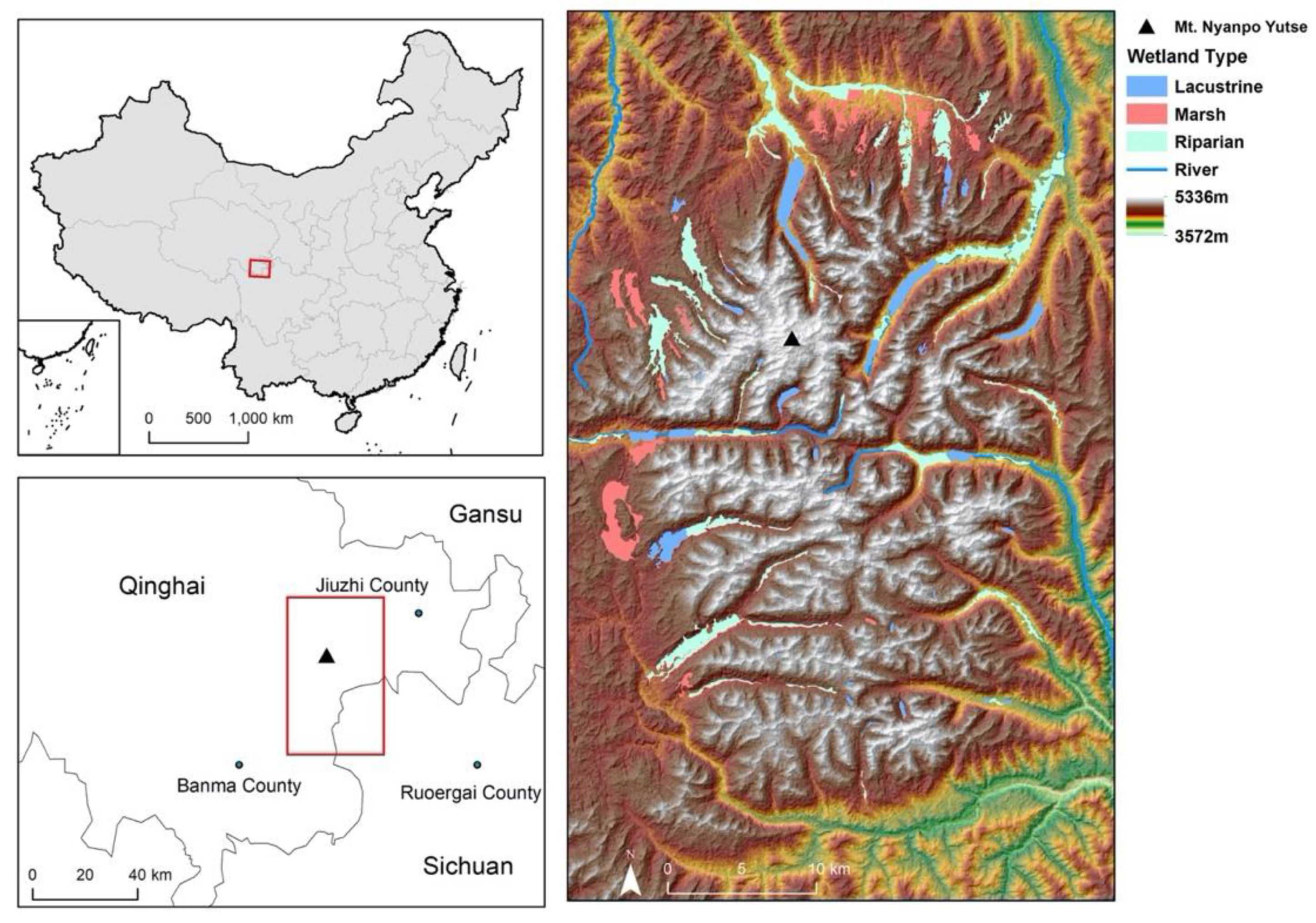
2.1. Regional Setting

Located on the Eastern Tibetan Plateau, our study site (100°90′–101°40′E, 32°90′–33°55′N) is a geomorphologically unique region surrounding Mt. Nyanpo Yutse (5368 m) on the border between Qinghai and Sichuan provinces, China (Figure 1). The region is characterized by an 820 km² granite dome rising 500–800 m above the surrounding peneplain, with the highest peaks above 5100 m still covered by 5.2 km² of modern glaciers [34]. Multiple Pleistocene glaciations deeply incised into granite batholith, leaving a distinctive glacial landform of U-shaped valleys, cirque lakes, and granite moraines. Below the near-vertical granite cliffs, alpine meadow covers much of the aeolian sandy silt between 3500 and 4300 m, providing pasture for nomadic herders who have been migrating across the region for at least 2200 years, based on palaeoecological records [35]. The region’s climate is controlled by the East Asian monsoon and can be divided into cold and warm seasons, with an annual mean temperature of 0.1 °C and an annual mean precipitation of 760 mm [31]. It is one of the wettest regions in Qinghai Province, but ~80% of the annual precipitation occurs from May to October, making the cold season very dry (Figure 2). The steep elevation and climate gradients in the region lead to a diversity of micro ecosystems, providing habitats for some endangered species such as snow leopard (Panthera uncia), Tibetan bunting (Emberiza koslowi), black-necked crane (Grus nigricolis), and an endemic Himalayan poppy (Meconopsis barbiseta) [36].

Hydrographically, Mt. Nyanpo Yutse is part of the NW–SE Bayan Har Mountains that divide the Yangtze River watershed to the south and the Yellow River watershed to the north. With elevation gradually decreasing from the center of the study region to the periphery, rivers radiate outward along the glacial trough valleys. At the flat bottom of the valleys or where moraines impede water flow, wetlands may develop. Based on their geological settings, we classified wetlands in our study area into three types: (1) “lacustrine wetlands”, which surround open cirque lakes that are directly controlled by the water level in the lakes; (2) “riparian wetlands”, which develop along the riverbed of braided rivers at the bottom of the glacial trough valleys or on alluvial fans at valley openings; and (3) “marsh wetlands” with thick peat layers, which are found in glacial basins to the north and east of the study region (see the right panel of Figure 1 for details). In this study, we only focused on riparian wetlands and marsh lands since the narrow width of lacustrine wetlands around the lake often makes them difficult to separate from open water on medium-resolution satellite images.

Given that there is no significant surface water flow into the region, the incoming water is almost entirely from rain, snowmelt, and glaciers (Figure 3). As modern glaciers cover less than 1% of the study region, we assumed their contribution to the regional water budget to be negligible. Thus, we considered rain and snowmelt to be the main sources. The main water sinks in our region are surface flow, underground flow, and evapotranspiration. However, without detailed ground monitoring data, we cannot reliably estimate the extent to which these variables have changed over the past decades. Thus, we focused only on evapotranspiration, with the assumption that the latter would be more directly influenced by climatic drivers such as temperature, wind speed, and relative humidity.

2.2. Analysis of Satellite-Based Evidence of Wetland Change

Our first goal was to quantify changes in wetland areas by conducting supervised classification of Landsat images over our study site (Path: 137, Row: 37). We acquired all Landsat TM, ETM, and OLI images captured between mid-July and mid-August from 1988 to 2017 and filtered the images by the percentage of cloud cover. Because of heavy clouds in the summers, we found only five usable images with light cloud cover over the wetlands of interest. These were captured by Landsat 5 TM on 16 August 1996; 14 August 2001; 6 August 2004; 27 July 2006; and 25 July 2011. All scenes were preprocessed to the study area’s extent, atmospherically corrected, calibrated to surface reflectance, and normalized to values between 0 and 1. We then applied Landsat QA bands to mask out the clouds and cloud shadows. Based on extensive fieldwork experience in the region and visual interpretation of a Landsat TM image from 2004, we created a training dataset consisting of six land-cover types: wetland, lake, bare rock, ice, meadow, and shrub. The numbers of training pixels for each class were approximately proportional to the area of the class, and a signature file was computed independently for each image over the same training regions. We used this training sample to train a maximum-likelihood classifier on bands 1–7 of each Landsat image, and applied the classifier to each image. The algorithm correctly separated bare rocks, glacier, lake, and meadow from other land-use types. Ancillary data were used to distinguish wetlands from upland shrub regions based on the similarity of their spectral signatures. For this purpose, we used 30 m ASTER GDEM to mask out all wetland pixels with an elevation above 4500 m or a slope greater than 20 degrees because surface water cannot easily be contained on sleep slopes, except under special geological settings [37]. We masked out all regions where there was a data gap in any of the images and counted the number of pixels classified as wetlands in each image. We then evaluated the accuracy of the classification by constructing confusion matrices against an independent test dataset and calculated Cohen’s kappa as an indicator of reliability.

Next, we examined potential changes in vegetation and water cycles within the wetlands. Due to extensive cloud cover, we apply synthetic aperture radar data to the problem, as it can provide information on water level and the texture of vegetation canopies regardless of cloudiness [38]. In this study, we utilized the Sentinel-1 GRD collection hosted on Google Earth Engine. This dataset has been preprocessed through a sequence of steps, including updating orbit metadata, border noise removal, thermal noise removal, radiometric calibration, and terrain correction using the protocols in Sentinel-1 Toolbox. The raw unitless backscatter coefficients were converted to normalized backscatter coefficients in dB [39]. We filtered the dataset to extract all images over the study area on the descending orbit acquired through the Interferometric Wide Swath mode. VV data has been available since October 2014. Using both ground-truth data and Landsat images, we manually traced out the contours of visible marsh and riparian wetlands (assuming that the boundaries of wetland stayed constant over time, which was supported by the Landsat data). We then calculated the time series of VV backscatter coefficients averaged over each type of wetland.

2.3. Analysis of Potential Climate Drivers of Wetland Change

In addition to collecting direct evidence of wetland change, we examined the potential climate factors that may drive wetland degradation. A significant challenge for analyzing climate trends in our study area was the paucity of ground monitoring data. The closest weather station is located at 25 km to the northwest at the Jiuzhi county seat, which has a daily record of temperature, precipitation, wind speed, relative humidity, and sunshine hours from 1959.

To improve the spatial resolution of climate records, we supplemented the ground observations with satellite data and modeling products. For temperature, we explored the CHIRTS_max gridded station-corrected satellite derived monthly-averaged daily maximum temperature [40], but we found the CHIRTS_max data contained anomalies and was inconsistent with ground observations in our area of interest. Thus, the single-point observation was determined to be our best estimate of regional temperature trends for our local-scale application. We employed monthly snow cover fraction data derived from MODIS observations to inform estimates of spring meltwater. MODIS snow covered area data were validated as having about 90% accuracy over the Tibetan Plateau [41].

As previous studies have shown that the increase in evapotranspiration associated with temperature rise is a likely driver of climate-induced degradation on the Tibetan Plateau, we took extra caution in constructing the evapotranspiration records in our study area. In this study, we examined three kinds of indicators: (1) “actual evapotranspiration” (ET_a), the amount of water evaporated from the vegetation within our study region; (2) “reference crop evapotranspiration” (ET_ref), the maximum amount of water capable of being evaporated from the soil and transpired from vegetation [42]; (3) “changes in phenology” because a longer growing season can be a potential driver of greater evapotranspiration.

For actual evapotranspiration, we examined the 10-day average actual evapotranspiration product of the Simplified Surface Energy Balance model parameterized (SSEBop), and the 8-day averaged actual evapotranspiration product from Atmosphere-Land Exchange Inverse model (ALEXI). Combining 10-day average MODIS thermal imagery surface temperature, PRISM data for air temperature, and reference evapotranspiration from GDAS, the SSEBop model provides a thermally based estimation of ET_a based on predefined, seasonal dynamic “hot” and “cold” boundary conditions unique for each pixel [43]. The ALEXI model incorporated a 7-day clear sky MODIS thermal dataset into a two-source land-surface representation model consisting of both soil and canopy to derive the evapotranspiration estimate [44]. For reference crop evapotranspiration, we used the daily average weather variables recorded by Jiuzhi meteorological station and the Penman-Monteith equation recommended by FAO to compute E_rc each day and calculated annual mean values. We did not use the pan-evaporation data at Jiuzhi meteorological station because of the inconsistent use of different evaporation pans at the meteorological station and the lack of accurate calibration data.

Finally, we examined phenology data to determine if the trend of lengthening the growing season might drive up water demand in our region of interest. We calculated the growing degree-days in our region of interest, which is defined as GDD = (T_max − T_min)/2 if (T_max − T_min)/2 > T_base or 0 if otherwise [45]. A base temperature T_base = 0 °C was selected as our study region lies in the cold climate region [46]. We also computed the normalized difference vegetation index (NDVI) over our study region using MODIS 16-day, clear sky observation. We studied the trends on specific days during the spring and fall to examine if there were an indication of advancement in spring green-up or delay in fall senescence.

3. Results

3.1. Wetland Area

Based on a supervised classification (Figure 4), the wetland area in our study region was 61.4 km², 63.9 km², 86.4 km², 63.9 km², and 77.9 km² in 1996, 2001, 2004, 2006, and 2011, respectively. The classification accuracies before and after filtering were evaluated in

Table 2. Confusion Matrix of Supervised Classification for Landsat 5 TM image in 2004.

	Wetland	Lake	Rock	Meadow	Shrub	Total	User’s Accuracy
Wetland	78	0	0	4	7	89	0.88
Lake	0	34	0	0	0	34	1
Rock	1	8	80	0	0	89	0.90
Meadow	12	0	0	69	30	111	0.62
Shrub	2	0	0	0	28	30	0.93
Total	93	42	80	73	65	353
Producer’s Accuracy	0.84	0.81	1	0.95	0.43
Kappa	0.77

and

Table 3. Confusion Matrix After Filtering by Elevation and Slope for 2004 Image.

	Non-Wetland	Wetland	Total	User’s Accuracy
Non-Wetland	253	7	260	0.97
Wetland	18	75	93	0.81
Total	271	82	353
Producer’s Accuracy	0.93	0.91
Kappa	0.81

, using ground-truth points selected based on first-hand field knowledge and visual interpretation of a recent Sentinel-2 image. The Cohen’s kappa coefficient was 0.77 for all five land cover types (ice was excluded because of the very small number of pixels available), and 0.81 for wetland/non-wetland after reclassification and filtering. These results were skewed by the varying degree of cloud cover in different scenes. In particular, the Landsat image from 2004 is the only cloud-free image, so it has a much larger number of effective training samples than the other images, which resulted in a greater number of pixels being classified as wetland. A comparison between wetland classification at the beginning and the end of the study period (1996 and 2011) suggests that there are no consistent spatial patterns of pixels indicating wetland gain or wetland loss, so the observed variations in the total area of pixels classified as wetland is more likely due to classification errors and cloud cover than actual changes in the wetland area (Figure 5). Comparing Landsat images in different years to our ground-truth data, we did not observe a visible change in the wetland boundary, suggesting that the actual area of wetlands may be mostly stable.

3.2. Wetland Vegetation and Water

Figure 6 displays the seasonal pattern of Sentinel-1 SAR backscattering coefficients of wetlands in the northern part of our study area. The red band displays time-averaged normalized backscattering coefficient in spring (15 March–15 April), the green band shows that for late spring (10 May–1 June), and the blue band shows that for summer (15 July–15 August). Note that all vegetated parts of the image have a bluish-green color, which suggests increased backscattering during periods of vegetation growth. In particular, the wetland has a brighter color than the surrounding area, suggesting that during the growing season the backscatter is higher in the water-flooded wetland than the adjacent grassland. This is not surprising given the presence of a microwave double bounce between wetland water and hydrophytes. Therefore, a higher backscatter coefficient is indicative of the presence of water and/or hydrophyte in the wetland. This seasonal cycle is clear in the normalized VV backscattering coefficients averaged across all the marsh and riparian wetlands in our study region (Figure 7). However, the data did not demonstrate a multi-year trend that would indicate interannual changes in wetland content or vegetation structure.

3.3. Meteorological Record

The average daily mean temperature recorded at Jiuzhi increased by 2.36 °C from 1959 to 2017, with an average rate of increase of 0.04 °C per year (F_1,56 = 150.3, p < 0.0001). During the same period, the average daily min temperature increased by 2.98 °C (F_1,56 = 143.5, p < 0.0001), whereas the average daily max temperature increased by only 1.25 °C (F_1,56 = 14.9, p = 0.0003). Furthermore, while there was a significant increase in January max temperature (F_1,56 = 5.4, p = 0.01) the maximum temperature increase in July was not significant (F_1,56 = 3.45, p = 0.07). The increase in minimum temperature was significant in both January (F_1,57 = 40.69, p < 0.0001) with rate of 0.077 °C per year and July (F_1,57 = 9.64, p = 0.003) with a rate of 0.028 °C per year. However, CHIRTS_max data did not show a significant increase in daily maximum temperature averaged across all months from 1983 to 2016 in the northern part of the study region, including the location of the meteorological station. A positive trend is observed in CHIRTS_max for January daily maximum temperature (p < 0.05), and the rate of increase gradually declines from 0.046 °C per year in the southwest to 0.025 °C per year in the northeast of the study region. During the same period, there was no significant change in annual total precipitation (F_1,56 = 1.44, p = 0.24), but the relative humidity had a significant decline (F_1,56 = 14.57, p = 0.0003). The wind speed showed an increasing trend from around 1.8 to 2.4 m/s from the 1970s to 1980s, and it fell back to about 1.7 m/s at the beginning of the 2000s before increasing slightly in the late 2000s (Figure 8).

3.4. Snow Cover Fraction

Trends in MODIS snow cover fraction from 2000 to early 2019 are presented in Figure 9. The monthly cover snow cover in our region showed variations from year to year, yet there was no multiannual trend in the data (F_1,16 = 0.57, p = 0.46). Figure 9B–D shows the timing of snow cover reduction in spring, which would affect the rate of meltwater influx, but, again, there is not a clear multiannual trend.

3.5. Evapotranspiration Trends

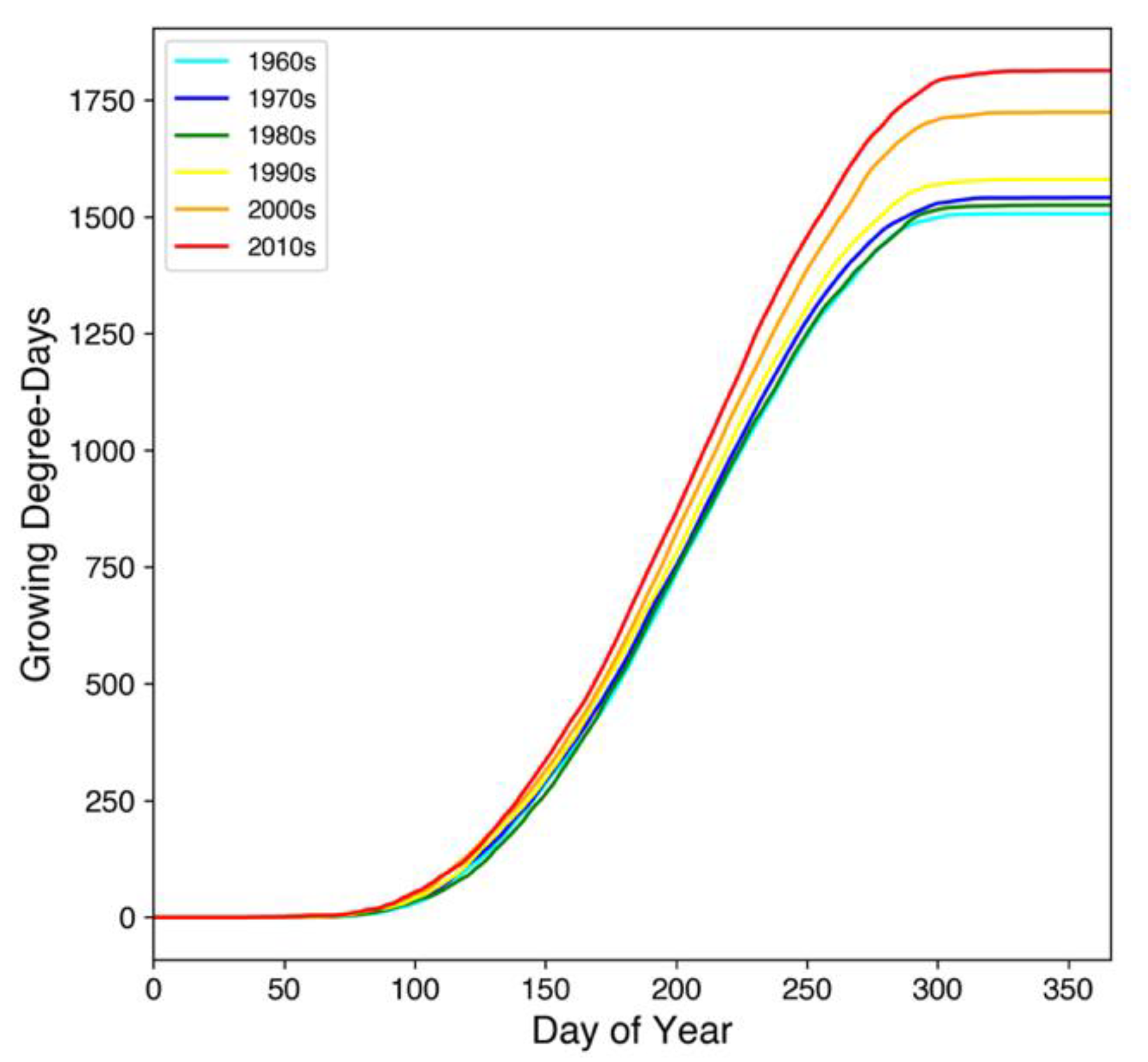
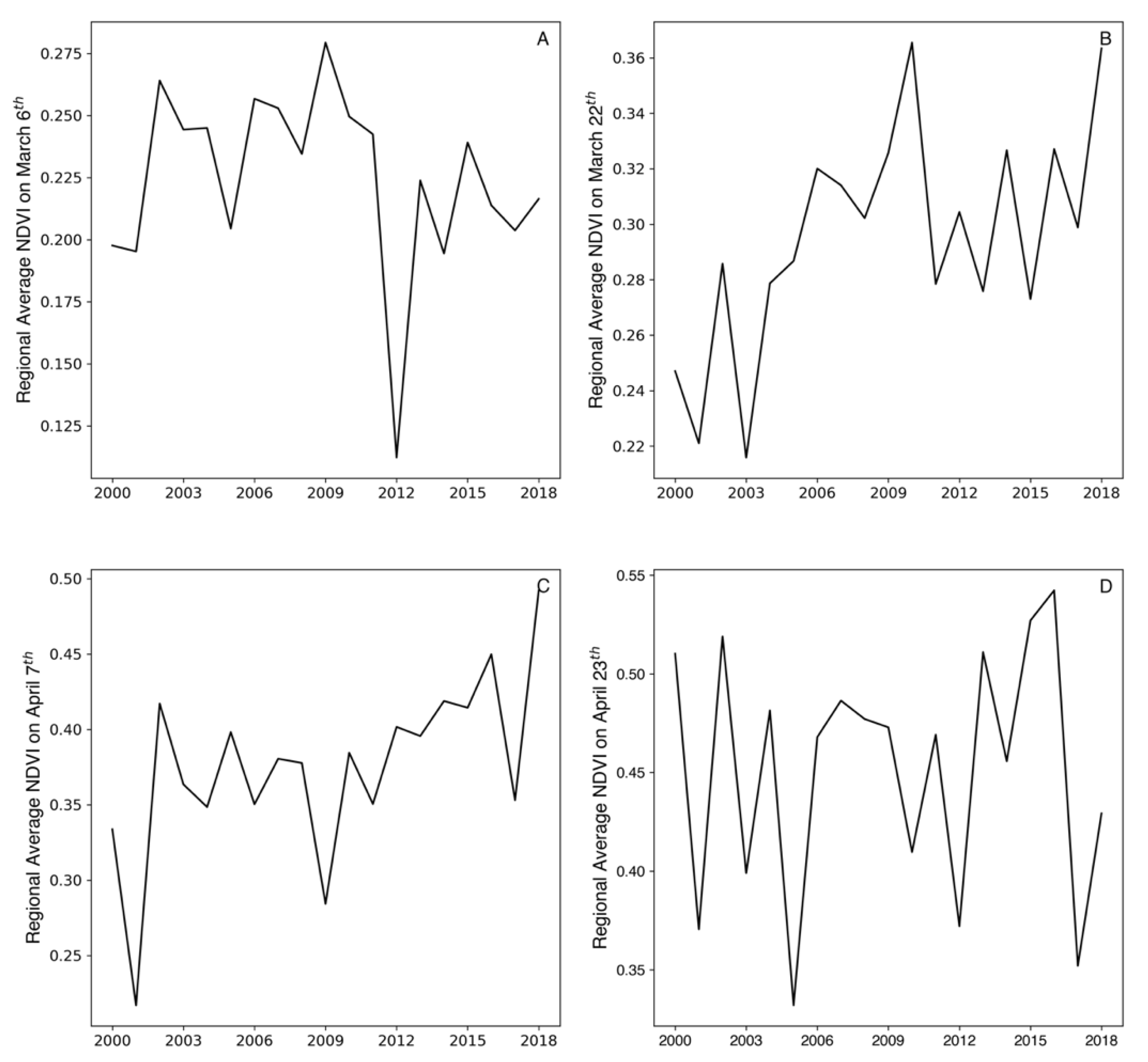
Regional average evapotranspiration modeled by ALEXI from 2003 to 2016 is presented in Figure 10. While the data suggested a clear seasonal cycle, there was no pattern in the annual total evapotranspiration (F_1,12 = 0.01, p = 0.94), which varied from 380 to 490 mm during the study period. The SSEBop model (Figure 11), on the other hand, showed regional average evapotranspiration for only about half of the ALEXI model’s estimate, averaging from 130 to 230 mm per year. Note that from April to May 2005, there were records with abnormally high evapotranspiration values. However, a cross-check with the weather data in this period revealed no anomalous deviation in temperature, precipitation, or wind speed compared with the multiannual mean. If we replace the anomalies with five-year medians, then there is a significant positive trend (F_1,16 = 4.48, p = 0.05). The reference crop evapotranspiration is about twice the actual evapotranspiration estimated by ALEXI and about four times the actual evapotranspiration estimated by SSEBop. There is a significant positive trend in the reference crop evapotranspiration (F_1,56 = 16.4, p = 0.0002) between 1959 and 2017 (Figure 12). The reference crop is evapotranspiration positively correlated with annual average daily maximum temperature (F_1,56 = 62.5, p < 0.0001), daily maximum temperature (F_1,56 = 6.47, p = 0.014), daily mean temperature (F_1,56 = 15.7, p = 0.0002), and sunshine hours (F_1,56 = 69.2, p < 0.0001). Furthermore, the reference crop evapotranspiration is negatively correlated with relative humidity (F_1,56 = 37.5, p < 0.0001) but not with wind speed (F_1,56 = 0.00, p = 0.98).

3.6. Phenology

Between 1960 and 2017, the total growing degree-days in our region of interest increased from 1506 in the 1960s to 1813 in the 2010s. The decade-averaged growing-degree days remained mostly the same from the 1960s to 1980s, but it dramatically increased in the 1990s. The greatest shift in growing-degree days happened between the 1990s and 2000s, where there was a sharp increase from 1580 to 1723 degree-days (Figure 13).

The MODIS 16-day averaged NDVI recorded between 2000 and 2018 suggested an advancement in spring phenology that was reflected by an upward trend in interannual NDVI on specific dates during the spring. A rising trend was observed in NDVI recorded on 22 March (F_1,17 = 9.43, p = 0.007) and 7 April (F_1,17 = 8.57, p = 0.0094) but not on 6 March (F_1,17 = 0.73, p = 0.40) or 23 April (F = 0.03, p = 0.87). Thus, the rising trend was only observed during an approximate 32-day period during the early phase of the greening-up but not during the entire spring (Figure 14). A delay in fall phenology, however, was not observed in the data (Figure 15) as no NDVI trend was observed on 13 August (F_1,17 = 0.01, p = 0.93), 29 August (F_1,17 = 0.19, p = 0.67), 14 September (F_1,17 = 0.14, p = 0.71), or 30 September (F_1,17 = 0.13, p = 0.72).

4. Discussion

This study was motivated by local herder reports of wetland degradation in our study area. Based on these reports, we expected to find evidence in optical or radar satellite images of changes in wetland area or water content or shifting vegetation structure in the wetland that would match the ground reports. Given previous studies on climate trends on the Tibetan Plateau, we also expected to identify potential climate drivers to explain the reported changes. However, the Landsat records showed no substantive change in our study area. The C-band SAR images of Sentinel-1 were only available for recent years, but they also indicated no significant interannual difference in the backscatter coefficients of the wetland. Thus, remote sensing presented a different picture of the wetlands than the testimonies from local herders.

On the other hand, the climate record showed a mixed result that partially supported the existence of climate factors that may drive up water demand in the wetlands. Although we observed no net change in precipitation in approximately the last 60 years or the snow cover fraction over the last 20 years, we did see some evidence of rising evapotranspiration and an extension of the growing season. In particular, one of the two satellite-based diagnostic evapotranspiration models showed an upward trend in actual evapotranspiration, and the calculated annual reference crop evapotranspiration shows a total of 55 mm increase from 1959 to 2017. At the same time, both MODIS NDVI and the growing degree-days data point to a lengthening of the growing season, which might be another factor that drives up the water demand in the wetland.

Analysis of Climate Trends

From a climate perspective, the study region’s trends exemplified the widespread warming patterns on the Tibetan Plateau. The magnitude of temperature rise at Jiuzhi was much more significant in the winter than in the summer, which is in agreement with earlier studies that found the winter warming (0.32 °C per decade) to be twice that of the annual mean temperature (0.16 °C per decade) [3]. We also found a larger and more consistent increase in the daily minimum temperature than in the daily maximum, suggesting that warming had a more substantial effect on reducing the net radiative cooling at night.

The trends in reference crop evapotranspiration (E_rc) suggest that the evapotranspiration in our region is temperature-limited rather than precipitation-limited, since (1) there is a strong correlation between E_rc and temperature, but no correlation between E_rc and precipitation; and (2) there is a net water surplus in the region because the estimated evapotranspiration, regardless of which estimate approach is used, is lower than the total precipitation. Thus, an increasing temperature would be expected to lead to an increase in evapotranspiration. Positive trends in ET were observed in wetlands in the wet areas of the Tibetan Plateau, such as the Zoige basin. In contrast, a negative trend in ET was observed in wetlands in the hinterland of the Tibetan Plateau, such as the Maidika wetland and Qiangtang plateau where evapotranspiration is constrained by soil moisture [14,47]. This increasing trend, however, is not consistent with an overall trend of reference evapotranspiration across the Tibetan Plateau or Eastern China, in general, where decreasing evapotranspiration is considered to be related to decreasing wind speed caused by a decline in the intensity of regional monsoon circulation and a decrease in the solar radiation [42,48,49]. In our study, evapotranspiration was found to be correlated with sunshine hours but did not correlate with wind speed despite its significant rise and decline over a period of three decades from 1970 to 2000. A combination of increasing temperature and decreasing relative humidity is the probable cause of a long-term increase in evapotranspiration.

It must be noted that the estimates for actual evapotranspiration from energy balance models should be evaluated with caution. The ALEXI dataset did not take account the effect of topography and elevation in its model [50]. The SSEBop model, while it did involve correction for elevation, still performed less optimally in regions with complex terrain. As its developer suggests, the high variations in ET fraction over mountainous regions revealed the inherent difficulty of capturing radiation and heat transfer process on steep slopes. This limitation continues to be an area where more research is needed [51]. However, a comparison between our study region with a recent study in Zoige wetland (100–150 km to the east with an elevation around 700–900 m lower than our region) offers some very general evidence that the estimates of the model fall within a reasonable range. The authors of that study estimated the evaporation fraction (Kc)—the ratio between actual evapotranspiration and reference evapotranspiration—to be 0.40, 0.73, and 0.60 in grassland and 0.70, 1.09, 0.62 for peatland at Maqu county during the initial, mid-, and end-section of the growing season [14]. Given that the Maqu weather station is only 83 km to the northeast and 150 m lower in elevation than Jiuzhi weather station, we may assume that these values applied to the evaporation fraction for wetland and grassland near the Jiuzhi township. However, it would be challenging to determine actual evapotranspiration using the single evaporation fraction approach because the weather records at Jiuzhi township may not be representative for wetlands located in higher elevation regions.

Our study also provided some insight into the debate on how climate change affects spring phenology on the Tibetan Plateau. One hypothesis that gained traction in the early 2010s is that strong warming in the winter will slow the fulfillment of chilling requirements for plants to germinate, thereby causing delays in spring phenology [52]. At the same time, there was a competing hypothesis suggesting that a continuous advancement in spring phenology with more substantial advancement at higher altitude [23,46,53]. Our study seemed to support the second hypothesis although we did not observe a corresponding delay in the fall phenology. While some researchers have pointed out the observed increase in spring NDVI might be a false signal caused by decreasing snow cover [54], this did not appear to be the case since we did not observe a trend in the snow cover fraction during the same period.

Uncertainties in the Temporal and Spatial Scale

It should be noted that the purpose of this study was not to validate or disprove local herder’s observations but to provide information that may support local conservation actions. In particular, the mismatch between the satellite records and the accounts from the local herders illustrated the importance of being aware of spatial and temporal scales when combining evidence from different sources to evaluate local environmental change. In the local herders’ oral accounts, wetland degradation was described in phenomena like whether yaks can walk across a patch of marshland without sinking into the peat. However, converting these claims into hypotheses verifiable by satellite images was challenging because (1) the described phenomenon may happen on a very fine-grained scale below the resolution of satellite images like Landsat; (2) the specific year and season of the observation was unknown, while the record of optical remote sensing record contains many gaps due to severe cloud coverage; (3) the effective resolution of vegetation change or water content often requires hyperspectral images or active remote sensing, yet many of these products do not have a record long enough to trace the wetland changes on a decadal scale.

The recent developments of high-resolution optical sensors and the increasing availability of SAR imagery has led to advances in characterizing water levels in seasonally inundated vegetation [38]. Our study demonstrated that the time-series of Sentinel-1 image is capable of capturing seasonal trends in wetlands and differentiating the vegetation within the wetland from that of the surrounding pastures. While the length of the Sentinel record is not presently sufficient to reveal long-term changes in wetlands in our study, it is expected that we may have the potential to characterize details of changes happening within the wetlands as the record grows in length. However, remote-sensing technology cannot replace the need for in situ measurements of hydrological and climate variables, and accurate ground-truth data is needed to improve the reliability of climate models in topographically complex areas. While recognizing the promise of remote-sensing technology for large-scale wetland mapping, researchers should be aware of the need to verify satellite-derived data with ground observations and of relevant opportunities and limitations when applying space-borne observations to the ground.

5. Conclusions

Local herders in our study region reported significant degradation to local wetlands over the past 30 years. However, we were unable to detect changes associated with local wetland degradation. Our study, using various publicly available remote sensing datasets, did not provide evidence corresponding to a reduction in local wetland area between 1996 and 2010 or interannual vegetation and water changes in the wetlands from 2015 to 2020. In the broader context of rapid warming on the Tibetan Plateau, we found within our study region an increase in evapotranspiration and an extension of the growing season, which might have raised water demand in the local wetlands and contributed to the reported degradation. The discrepancies between wetland changes observed on the ground and trends observed from the satellites show the challenges of characterizing climate-related wetland changes at scales relevant to local conservation actions. These limitations highlight the need for in situ studies of climate and hydrological changes in topographically complex regions on the Tibetan Plateau, as well as an examination of high resolution commercial satellite imagery because data from these platforms are becoming more accessible to budget-constrained conservation organizations.

References

1. Bullock, A.; Acreman, M. The Role of Wetlands in the Hydrological Cycle. Hydrol. Earth Syst. Sci. 2003, 7, 358–389. [Google Scholar] [CrossRef] [Green Version]
2. Zhao, Z.; Zhang, Y.; Liu, L.; Liu, F.; Zhang, H. Recent Changes in Wetlands on the Tibetan Plateau: A Review. J. Geogr. Sci. 2015, 25, 879–896. [Google Scholar] [CrossRef] [Green Version]
3. Liu, X.; Chen, B. Climatic Warming in the Tibetan Plateau during Recent Decades. Int. J. Climatol. 2000, 20, 1729–1742. [Google Scholar] [CrossRef]
4. Wang, B.; Bao, Q.; Hoskins, B.; Wu, G.; Liu, Y. Tibetan Plateau Warming and Precipitation Changes in East Asia. Geophys. Res. Lett. 2008, 35, 2–6. [Google Scholar] [CrossRef] [Green Version]
5. Zhang, Y.; Wang, G.; Wang, Y. Changes in Alpine Wetland Ecosystems of the Qinghai-Tibetan Plateau from 1967 to 2004. Environ. Monit. Assess. 2011, 180, 189–199. [Google Scholar] [CrossRef] [Green Version]
6. Xue, Z.; Zhang, Z.; Lu, X.; Zou, Y.; Lu, Y.; Jiang, M.; Tong, S.; Zhang, K. Predicted Areas of Potential Distributions of Alpine Wetlands under Different Scenarios in the Qinghai-Tibetan Plateau, China. Glob. Planet. Change 2014, 123, 77–85. [Google Scholar] [CrossRef]
7. Liu, D.; Xu, M. Dynamic Changes of the Alpine Wetlands in Tibet, China. In Proceedings of the IGARSS, Valencia, Spain, 22–27 July 2018; pp. 9229–9232. [Google Scholar]
8. Erwin, K.L. Wetlands and Global Climate Change: The Role of Wetland Restoration in a Changing World. Wetl. Ecol. Manag. 2009, 17, 71–84. [Google Scholar] [CrossRef]
9. Li, W.; Xu, J. Typical Alpine Wetland Landscape Changes in Eastern Tibetan Plateau under Climate Change over 15 Years. Int. Geosci. Remote Sens. Symp. 2012, 4907–4910. [Google Scholar] [CrossRef]
10. Kang, S.; Xu, Y.; You, Q.; Flügel, W.A.; Pepin, N.; Yao, T. Review of Climate and Cryospheric Change in the Tibetan Plateau. Environ. Res. Lett. 2010, 5. [Google Scholar] [CrossRef]
11. Li, Z.; Xu, J.; Shilpakar, R.L.; Ma, X. Mapping Wetland Cover in the Greater Himalayan Region: A Hybrid Method Combining Multispectral and Ecological Characteristics. Environ. Earth Sci. 2014, 71, 1083–1094. [Google Scholar] [CrossRef]
12. Cheng, G.; Wu, T. Responses of Permafrost to Climate Change and Their Environmental Significance, Qinghai-Tibet Plateau. J. Geophys. Res. Earth Surf. 2007, 112, 1–10. [Google Scholar] [CrossRef] [Green Version]
13. Gao, J.; Li, X.L.; Cheung, A.; Yang, Y.W. Degradation of Wetlands on the Qinghai-Tibet Plateau: A Comparison of the Effectiveness of Three Indicators. J. Mt. Sci. 2013, 10, 658–667. [Google Scholar] [CrossRef] [Green Version]
14. Li, Z.; Gao, P.; Hu, X.; Yi, Y.; Pan, B.; You, Y. Coupled Impact of Decadal Precipitation and Evapotranspiration on Peatland Degradation in the Zoige Basin, China. Phys. Geogr. 2020, 41, 145–168. [Google Scholar] [CrossRef]
15. Luo, C.; Hao, M.; Li, Y.; Tong, L. Monitoring the Changes of Wetlands in the Source Region of Three Rivers with Remote Sensing Data from 1976 to 2013. In Proceedings of the 2016 4th International Workshop on Earth Observation and Remote Sensing Applications (EORSA), Guangzhou, China, 4–6 July 2016; pp. 198–201. [Google Scholar]
16. Nie, Y.; Li, A. Assessment of Alpine Wetland Dynamics from 1976–2006 in the Vicinity of Mount Everest. Wetlands 2011, 31, 875–884. [Google Scholar] [CrossRef]
17. Qiu, P.; Wu, N.; Luo, P.; Wang, Z.; Li, M. Analysis of Dynamics and Driving Factors of Wetland Landscape in Zoige, Eastern Qinghai-Tibetan Plateau. J. Mt. Sci. 2009, 6, 42–55. [Google Scholar] [CrossRef] [Green Version]
18. Shen, G.; Yang, X.; Jin, Y.; Xu, B.; Zhou, Q. Remote Sensing and Evaluation of the Wetland Ecological Degradation Process of the Zoige Plateau Wetland in China. Ecol. Indic. 2019, 104, 48–58. [Google Scholar] [CrossRef]
19. Wan, W.; Xiao, P.; Feng, X.; Li, H.; Ma, R.; Duan, H.; Zhao, L. Monitoring Lake Changes of Qinghai-Tibetan Plateau over the past 30 Years Using Satellite Remote Sensing Data. Chinese Sci. Bull. 2014, 59, 1021–1035. [Google Scholar] [CrossRef]
20. Zhang, W.; Yi, Y.; Song, K.; Kimball, J.S.; Lu, Q. Hydrological Response of Alpine Wetlands to Climate Warming in the Eastern Tibetan Plateau. Remote Sens. 2016, 8, 336. [Google Scholar] [CrossRef] [Green Version]
21. Yu, K.F.; Lehmkuhl, F.; Falk, D. Quantifying Land Degradation in the Zoige Basin, NE Tibetan Plateau Using Satellite Remote Sensing Data. J. Mt. Sci. 2017, 14, 77–93. [Google Scholar] [CrossRef]
22. Hu, G.; Dong, Z.; Wei, Z.; Lu, J. Land Use and Land Cover Change Monitoring in the Zoige Wetland by Remote Sensing. In Proceedings SPIE Volume 7841, In Proceedings of the 6th International Symposium on Digital Earth: Data Processing and Applications, Beijing, China, 9–12 September 2009; International Society for Optics and Photonics: Bellingham, WA, USA, 2010; p. 78410V. [Google Scholar]
23. Kang, X.; Hao, Y.; Cui, X.; Chen, H.; Huang, S.; Du, Y.; Li, W.; Kardol, P.; Xiao, X.; Cui, L. Variability and Changes in Climate, Phenology, and Gross Primary Production of an Alpine Wetland Ecosystem. Remote Sens. 2016, 8, 391. [Google Scholar] [CrossRef] [Green Version]
24. Guang-Yin, H.; Zhi-Bao, D.; Jun-Feng, L.; Chang-Zhen, Y. Driving Forces of Land Use and Land Cover Change (LUCC) in the Zoige Wetland, Qinghai-Tibetan Plateau. Sci. Cold Arid Reg. 2012, 4, 422. [Google Scholar] [CrossRef] [Green Version]
25. Li, J.; Wang, W.; Hu, G.; Wei, Z. Changes in Ecosystem Service Values in Zoige Plateau, China. Agric. Ecosyst. Environ. 2010, 139, 766–770. [Google Scholar] [CrossRef]
26. Foggin, J.M. Environmental Conservation in the Tibetan Plateau Region: Lessons for China’s Belt and Road Initiative in the Mountains of Central Asia. Land 2018, 7, 52. [Google Scholar] [CrossRef] [Green Version]
27. Yan, F.; Liu, X.; Chen, J.; Yu, L.; Yang, C.; Chang, L.; Yang, J.; Zhang, S. China’s Wetland Databases Based on Remote Sensing Technology. Chinese Geogr. Sci. 2017, 27, 374–388. [Google Scholar] [CrossRef] [Green Version]
28. General Schema of Sanjiangyuan National Park; National Development and Reform Commission: Beijing, China, 2018.
29. Shen, X.; Tan, J. Ecological Conservation, Cultural Preservation, and a Bridge between: The Journey of Shanshui Conservation Center in the Sanjiangyuan Region, Qinghai-Tibetan Plateau, China. Ecol. Soc. 2012, 17. [Google Scholar] [CrossRef]
30. Li, L. Alpine Habitat Dynamics and Avian Biodiversity in Different Land-use Regimes on the Eastern Tibetan Plateau; Springer: New York, NY, USA, 2017. [Google Scholar]
31. Li, L.; Fassnacht, F.E.; Storch, I.; Bürgi, M. Land-use Regime Shift Triggered the Recent Degradation of Alpine Pastures in Nyanpo Yutse of the Eastern Qinghai-Tibetan Plateau. Landsc. Ecol. 2017, 32, 2187–2203. [Google Scholar] [CrossRef]
32. Yeh, E.T. ‘How Can Experience of Local Residents be “Knowledge”?’ Challenges in Interdisciplinary Climate Change Research. Area 2016, 48, 34–40. [Google Scholar] [CrossRef]
33. Gallant, A.L.; Sadinski, W.; Brown, J.F.; Senay, G.B.; Roth, M.F. Challenges in Complementing Data from Ground-based Sensors with Satellite-derived Products to Measure Ecological Changes in Relation to Climate—lessons from Temperate Wetland-upland Landscapes. Sensors 2018, 18, 880. [Google Scholar] [CrossRef] [PubMed] [Green Version]
34. Zhang, C.; Mischke, S. A Lateglacial and Holocene Lake Record from the Nianbaoyeze Mountains and Inferences of Lake, Glacier and Climate Evolution on the Eastern Tibetan Plateau. Quat. Sci. Rev. 2009, 28, 1970–1983. [Google Scholar] [CrossRef]
35. Schlütz, F.; Lehmkuhl, F. Holocene Climatic Change and the Nomadic Anthropocene in Eastern Tibet: Palynological and Geomorphological Results from the Nianbaoyeze Mountains. Quat. Sci. Rev. 2009, 28, 1449–1471. [Google Scholar] [CrossRef]
36. Environment and Culture of the Tibetan Plateau (Nyanpo Yutse Volume); China Tibetology Publishing House: Beijing, China, 2019.
37. Stein, E.D.; Mattson, M.; Fetscher, A.E.; Halama, K.J. Influence of Geologic Setting on Slope Wetland Hydrodynamics. Wetlands 2004, 24, 244–260. [Google Scholar] [CrossRef]
38. White, L.; Brisco, B.; Dabboor, M.; Schmitt, A.; Pratt, A. A Collection of SAR Methodologies for Monitoring Wetlands. Remote Sens. 2015, 7, 7615–7645. [Google Scholar] [CrossRef] [Green Version]
39. Sentinel-1 Algorithms. Available online: https://developers.google.com/earth-engine/sentinel1 (accessed on 10 October 2020).
40. Funk, C.; Peterson, P.; Peterson, S.; Shukla, S.; Davenport, F.; Michaelsen, J.; Knapp, K.R.; Landsfeld, M.; Husak, G.; Harrison, L.; et al. A high-resolution 1983–2016 TMAX Climate Data Record Based on Infrared Temperatures and Stations by the Climate Hazard Center. J. Clim. 2019, 32, 5639–5658. [Google Scholar] [CrossRef]
41. Pu, Z.; Xu, L.; Salomonson, V.V. MODIS/Terra Observed Seasonal Variations of Snow Cover over the Tibetan Plateau. Geophys. Res. Lett. 2007, 34, 1–6. [Google Scholar] [CrossRef] [Green Version]
42. Zhang, Y.; Liu, C.; Tang, Y.; Yang, Y. Trends in Pan Evaporation and Reference and Actual Evapotranspiration across the Tibetan Plateau. J. Geophys. Res. Atmos. 2007, 112, 1–12. [Google Scholar] [CrossRef]
43. Senay, G.B.; Bohms, S.; Singh, R.K.; Gowda, P.H.; Velpuri, N.M.; Alemu, H.; Verdin, J.P. Operational Evapotranspiration Mapping Using Remote Sensing and Weather Datasets: A New Parameterization for the SSEB Approach. J. Am. Water Resour. Assoc. 2013, 49, 577–591. [Google Scholar] [CrossRef] [Green Version]
44. Anderson, M.C.; Norman, J.M.; Mecikalski, J.R.; Otkin, J.A.; Kustas, W.P. A Climatological Study of Evapotranspiration and Moisture Stress Across the Continental United States Based on Thermal Remote Sensing: 1. Model Formulation. J. Geophys. Res. Atmos. 2007, 112, 1–17. [Google Scholar] [CrossRef]
45. McMaster, G.S.; Wilhelm, W.; Wilhelm, W.W. Growing Degree-days: One Equation, Two Interpretations. Agric. For. Meteorol. 1997, 87, 291–300. [Google Scholar] [CrossRef] [Green Version]
46. Liu, L.; Liu, L.; Liang, L.; Donnelly, A.; Park, I.; Schwartz, M.D. Effects of Elevation on Spring Phenological Sensitivity to Temperature in Tibetan Plateau Grasslands. Chin. Sci. Bull. 2014, 59, 4856–4863. [Google Scholar] [CrossRef]
47. Wang, R.; He, M.; Niu, Z. Responses of Alpine Wetlands to Climate Changes on the Qinghai-Tibetan Plateau Based on Remote Sensing. Chin. Geogr. Sci. 2020, 30, 189–201. [Google Scholar] [CrossRef]
48. Gao, G.; Chen, D.; Ren, G.; Chen, Y.; Liao, Y. Spatial and Temporal Variations and Controlling Factors of Potential Evapotranspiration in China: 1956–2000. J. Geogr. Sci. 2006, 16, 3–12. [Google Scholar] [CrossRef]
49. Chen, S.; Liu, Y.; Axel, T. Climatic Change on the Tibetan Plateau: Potential Evapotranspiration Trends from 1961–2000. Clim. Change 2006, 76, 291–319. [Google Scholar] [CrossRef]
50. Anderson, M.C.; Norman, J.M.; Mecikalski, J.R.; Otkin, J.A.; Kustas, W.P. A Climatological Study of Evapotranspiration and Moisture Stress Across the Continental United States Based on Thermal Remote Sensing: 2. Surface Moisture Climatology. J. Geophys. Res. Atmos. 2007, 112. [Google Scholar] [CrossRef]
51. Senay, G.B.; Budde, M.E.; Verdin, J.P. Enhancing the Simplified Surface Energy Balance (SSEB) Approach for Estimating Landscape ET: Validation with the METRIC Model. Agric. Water Manag. 2011, 98, 606–618. [Google Scholar] [CrossRef]
52. Yu, H.; Luedeling, E.; Xu, J. Winter and Spring Warming Result in Delayed Spring Phenology on the Tibetan Plateau. Proc. Natl. Acad. Sci. USA 2010, 107, 22151–22156. [Google Scholar] [CrossRef] [PubMed] [Green Version]
53. Zhang, G.; Zhang, Y.; Dong, J.; Xiao, X. Green-up Dates in the Tibetan Plateau Have Continuously Advanced from 1982 to 2011. Proc. Natl. Acad. Sci. USA 2013, 110, 4309–4314. [Google Scholar] [CrossRef] [PubMed] [Green Version]
54. Wang, T.; Peng, S.; Lin, X.; Chang, J. Declining Snow Cover May Affect Spring Phenological Trend on the Tibetan Plateau. Proc. Natl. Acad. Sci. USA 2013, 110, E2854–E2855. [Google Scholar] [CrossRef] [Green Version]
Figure 1. Maps of the study area. The map on the right shows the locations of three types of wetlands based on manual classification from Landsat remote sensing images. Lacustrine wetlands refer to the open water of cirque lakes and the surrounding semi-submerged ground. Marsh wetlands are wetlands distributed along the banks of rivers and cover the bottom of the glacial valleys.
Remotesensing 13 01484 g001
Figure 2. Thirty-Year Average of Monthly Mean Temperature and Precipitation reported by the weather station at Jiuzhi county (elevation 3630 m), 25 km to the northeast of our study site.
Remotesensing 13 01484 g002
Figure 3. A simplified diagram of water sources and water sink in our study. The boxes marked in blue are factors estimated in this study.
Remotesensing 13 01484 g003
Figure 4. (a) Maximum-likelihood classification results of Landsat 5 TM image over the study area on 6 August 2004. (b) The scatterplot of Landsat band 4 (near infrared) and band 6 (thermal infrared).
Remotesensing 13 01484 g004
Figure 5. Composite of wetland classification results on 16 August 1996 and 25 July 2011. Grey pixels represent areas classified as wetland in both 1996 and 2011, black pixels represent areas not classified as wetland in either year. Red pixels represent areas classified as wetland in 1996 but not 2011. Cyan pixels represent areas classified as wetland in 2011 but not 1996. White pixels are regions removed due to cloud cover.
Remotesensing 13 01484 g005
Figure 6. False color Sentinel-1 VV image showing distinctive seasonal hydrological and vegetation patterns of wetlands compared with the surrounding grassland in 2019 (top) and 2010 (bottom).
Remotesensing 13 01484 g006
Figure 7. Red: Time series of backscatter coefficients of VV bands averaged over all marsh wetlands (A) and riparian wetlands (B). Blue: Time series of backscatter coefficients of VV bands averaged over samples of grassland in the study region.
Remotesensing 13 01484 g007
Figure 8. Time Series of Weather Data at Jiuzhi Station.
Remotesensing 13 01484 g008
Figure 9. (A) MODIS snow cover fraction from March 2000 to February 2019. (BD) Time series for March, April and May respectively.
Remotesensing 13 01484 g009
Figure 10. (A) Annual mean daily average actual evapotranspiration modeled by ALEXI data from 2003 to 2017 (B) Daily ALEXI evapotranspiration on different date of year from 2003 to 2017, with darker lines representing more recent years.
Remotesensing 13 01484 g010
Figure 11. (A) Annual mean daily evapotranspiration from 2003 to 2020 (B) Daily SSEBop evapotranspiration on different date of year from 2003 to 2020, with darker lines representing more recent years.
Remotesensing 13 01484 g011
Figure 12. (A) Time series of reference crop evapotranspiration; (B) Relation between reference crop evapotranspiration and annual mean temperature.
Remotesensing 13 01484 g012
Figure 13. Cumulative growing degree-days by decades.
Remotesensing 13 01484 g013
Figure 14. Regional-averaged 16-day MODIS NDVI on selected dates in the spring.
Remotesensing 13 01484 g014
Figure 15. Regional-averaged 16-day MODIS NDVI on selected dates in the fall.
Remotesensing 13 01484 g015