
A Robust Prediction Model for Species Distribution Using Bagging Ensembles with Deep Neural Networks


School of Electrical Engineering, Korea University, 145 Anam-ro, Seongbuk-gu, Seoul 02841, Korea
*
Author to whom correspondence should be addressed.
Remote Sens. 2021, 13(8), 1495; https://0-doi-org.brum.beds.ac.uk/10.3390/rs13081495
Submission received: 26 February 2021
/
Revised: 9 April 2021
/
Accepted: 10 April 2021
/
Published: 13 April 2021
(This article belongs to the Special Issue Remote Sensing for Biodiversity Mapping and Monitoring)
Abstract
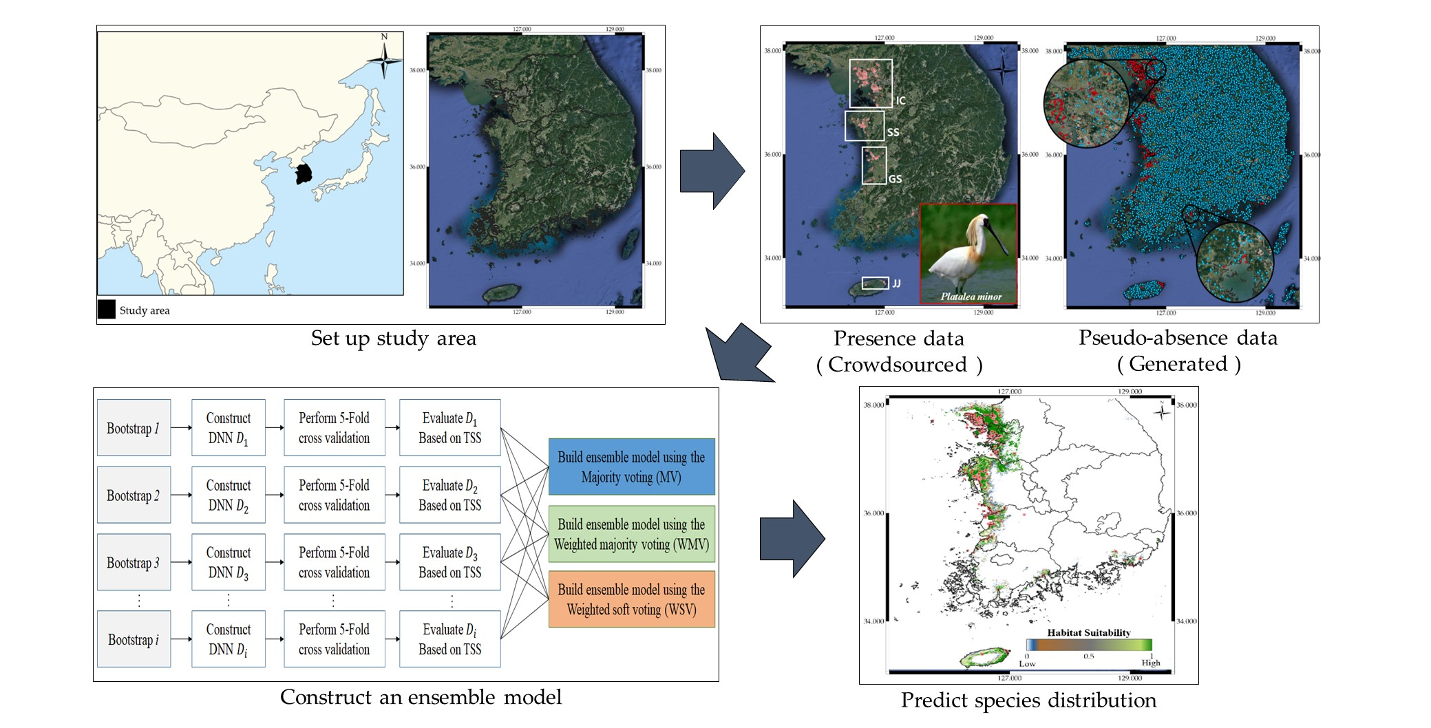
:Species distribution models have been used for various purposes, such as conserving species, discovering potential habitats, and obtaining evolutionary insights by predicting species occurrence. Many statistical and machine-learning-based approaches have been proposed to construct effective species distribution models, but with limited success due to spatial biases in presences and imbalanced presence-absences. We propose a novel species distribution model to address these problems based on bootstrap aggregating (bagging) ensembles of deep neural networks (DNNs). We first generate bootstraps considering presence-absence data on spatial balance to alleviate the bias problem. Then we construct DNNs using environmental data from presence and absence locations, and finally combine these into an ensemble model using three voting methods to improve prediction accuracy. Extensive experiments verified the proposed model’s effectiveness for species in South Korea using crowdsourced observations that have spatial biases. The proposed model achieved more accurate and robust prediction results than the current best practice models.

1. Introduction
Biodiversity is an indispensable asset for sustainable human life. Although biodiversity is vital to balance natural ecosystems, it has declined dramatically over the past few centuries [1,2]. Humans have consumed biological resources as raw food material, industrial products, and pharmaceutical resources [3,4,5], and their indiscriminate use, as well as and rapid environmental changes, have adversely affected biodiversity preservation [6]. For instance, changes in agricultural forms, residential development, and logging over the past decades have led to a 68% decline in the number of mammals, birds, reptiles, and amphibians worldwide between 1970 and 2016 [7]. Negative biodiversity changes can destroy stable ecosystem balances, and many ecologists have proposed strategies to efficiently maintain ecosystem balance, such as species protection laws and habitat preservation [8,9,10]. Many ecologists have addressed the importance of habitat preservation for species protection, because it is very difficult to restore a habitat’s original condition once it is destroyed. Various studies characterized habitats associated with species survival and predicted species viability in new locations [11,12,13]. Species distribution models (SDMs), also known as ecological niche models, habitat models, and range mapping, predict species distributions based on observational data for the species and the related environment. SDMs have become standard tools for ecological studies [14,15,16,17], greatly helping to understand the suitability of a particular species to a habitat and derive possible habitat candidates. Methodologies for constructing SDMs are typically classified into presence-only (PO) [18,19,20] and presence-absence (PA) [21,22,23,24] based SDMs. PO-based SDMs were widely used before the advent of PA-based SDMs, since they did not require absence data and provide a simple and fast assessment of environmental suitability at a given location, e.g., the surface range envelop (SRE) [25] and Bioclim [26] methods. PO-based models for constructing the environmental suitability model (ESM) were considered useful in terms of the intuitive understanding of a niche; they provide slightly different answers to ecological questions than those of the typical PA-based SDMs. That is, PO-based models have focused primarily on understanding the potential distribution of species from niches. In contrast, typical PA-based SDMs have focused much more on the realized distribution in the evaluation process [27,28]. Therefore, since these two models have different purposes, it is not appropriate to compare them quantitatively.
Recently, PA-based SDMs have emerged with the development of machine learning (ML) technology, making it possible to reflect relationships between various parameters in the prediction. Consequently, SDM capabilities have improved dramatically and provided a new perspective on ecological research. Starting with the generalized linear model (GLM) and generalized additive (GAM) model, various ML methods—such as maximum entropy (MAXENT), random forest (RF), and generalized boosted regression (GBM)—have been used to construct SDMs. [29,30,31,32,33,34,35]. Moreover, by incorporating the PA approach (PA-ML SDMs), SDM models can have their own feature learning process and model optimization strategy. Most works on PA-ML SDMs focused on selecting the ML model that best suits their purpose and finding the best configuration to improve the prediction performance of the realized distribution of a given species.
However, some critical issues remain to be addressed to achieve meaningful predictions using PA-ML SDMs. Typical PA-ML SDMs rarely considered strategies to generate pseudo-absence data, with most approaches generating pseudo-absence randomly. Thus, the pseudo-absence level was out of balance with the presence data, which negatively affected predictive performance. The neglect of the spatial distributions of PA data collected from citizen science databases can lead to bias because SDM prediction is strongly dependent on the spatial distribution of PA data. Species observations collected by citizen scientists are often biased and more aligned with citizen preferences than scientific objectives [36,37]. For instance, observation data tend to be prevalently collected near urban areas, where many citizen scientists live. Deep neural networks (DNNs) have achieved superb performance in diverse domains, including classification, translation, and prediction when enough data is available for model training. Even in SDM, DNNs could be used effectively to identify potential habitats [38] compared to traditional SDM approaches and overcome their shortcomings in prediction when sufficient data are available [39]. Moreover, the effectiveness of DNNs on SDM was evaluated based on various data sample sizes and layer configurations [40].
However, there are several critical issues that most previous DNN-based works on SDM have not considered: (1) Which method is more suitable for generating pseudo-absence data in the SDM process, (2) How to obtain enough observation data with relaxed spatial bias and generate a well-balanced dataset for SDM training, and (3) How to configure DNN to further improve SDM performance compared to the existing SDM approaches. In order to address these issues, in this paper, we propose a novel SDM model using a bootstrap aggregating (bagging) DNN ensemble. The main contributions of this paper are as follows.
- We investigate several bias-minimizing methods, including selecting valuable environmental features and generating bootstraps from PA datasets. We use variance inflation factor (VIF) analysis to select suitable environmental features and use random sampling with replacement to generate multiple bootstraps.
- We predict species distribution using our ensemble DNNs trained with generated bootstraps, three voting methods, and repeated cross-validation to ensure reliable results. The generated models were compared to state-of-the-art practical SDMs using five evaluation metrics.
The remainder of this paper is organized as follows. Section 2 describes the major steps required to construct the proposed model, and Section 3 shows experimental results to evaluate prediction performance and predicted species distribution visualizations. Section 4 provides an extensive discussion of the findings of the study, and Section 5 concludes the paper.
2. Methods
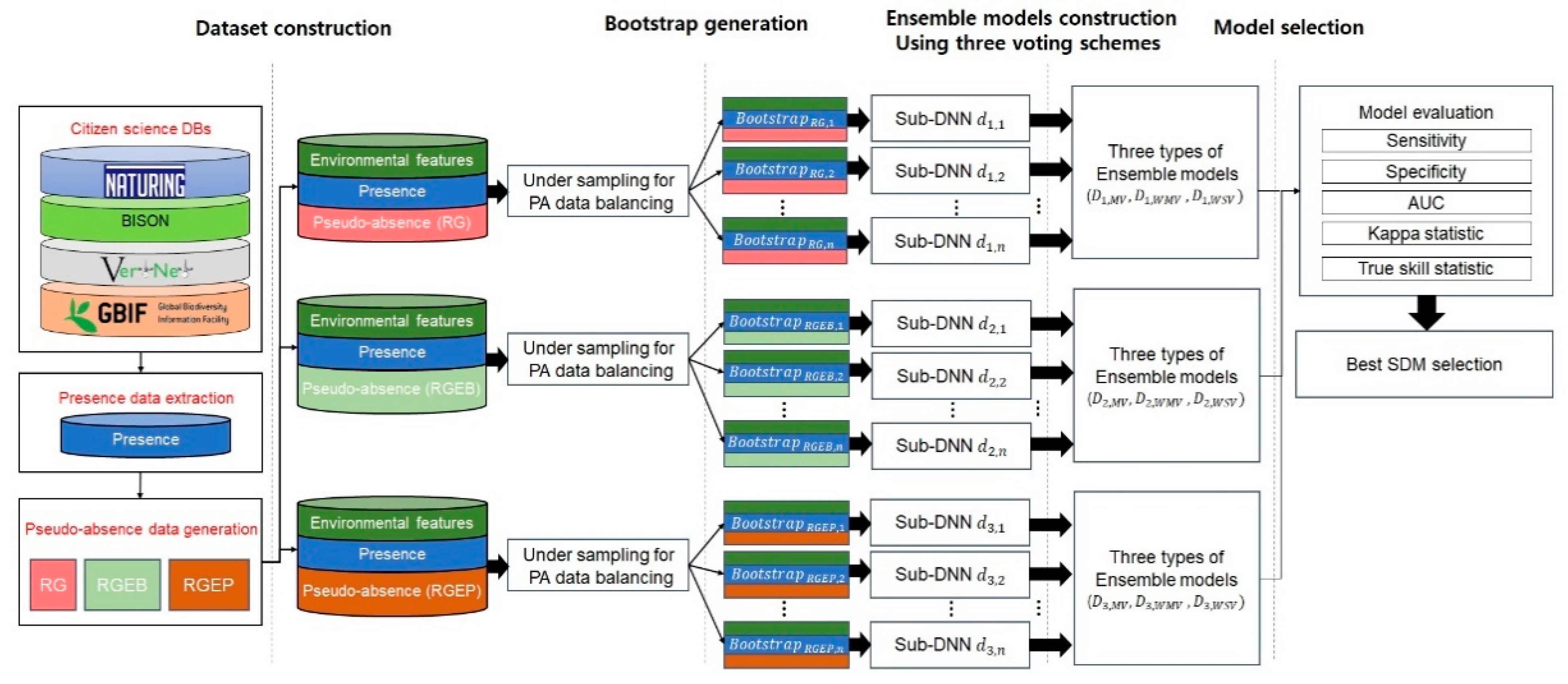
Figure 1 shows the proposed model’s overall structure. The model comprises three components: dataset construction, bootstrap generation, and ensemble model construction. We first describe how to construct the dataset, including species observation data, environmental variables, and pseudo-absence data. Then we explain how to generate bootstraps, considering PA data balancing, and finally we discuss how to train multiple DNNs and combine them to predict a particular species’ distribution.
2.1. Dataset Construction
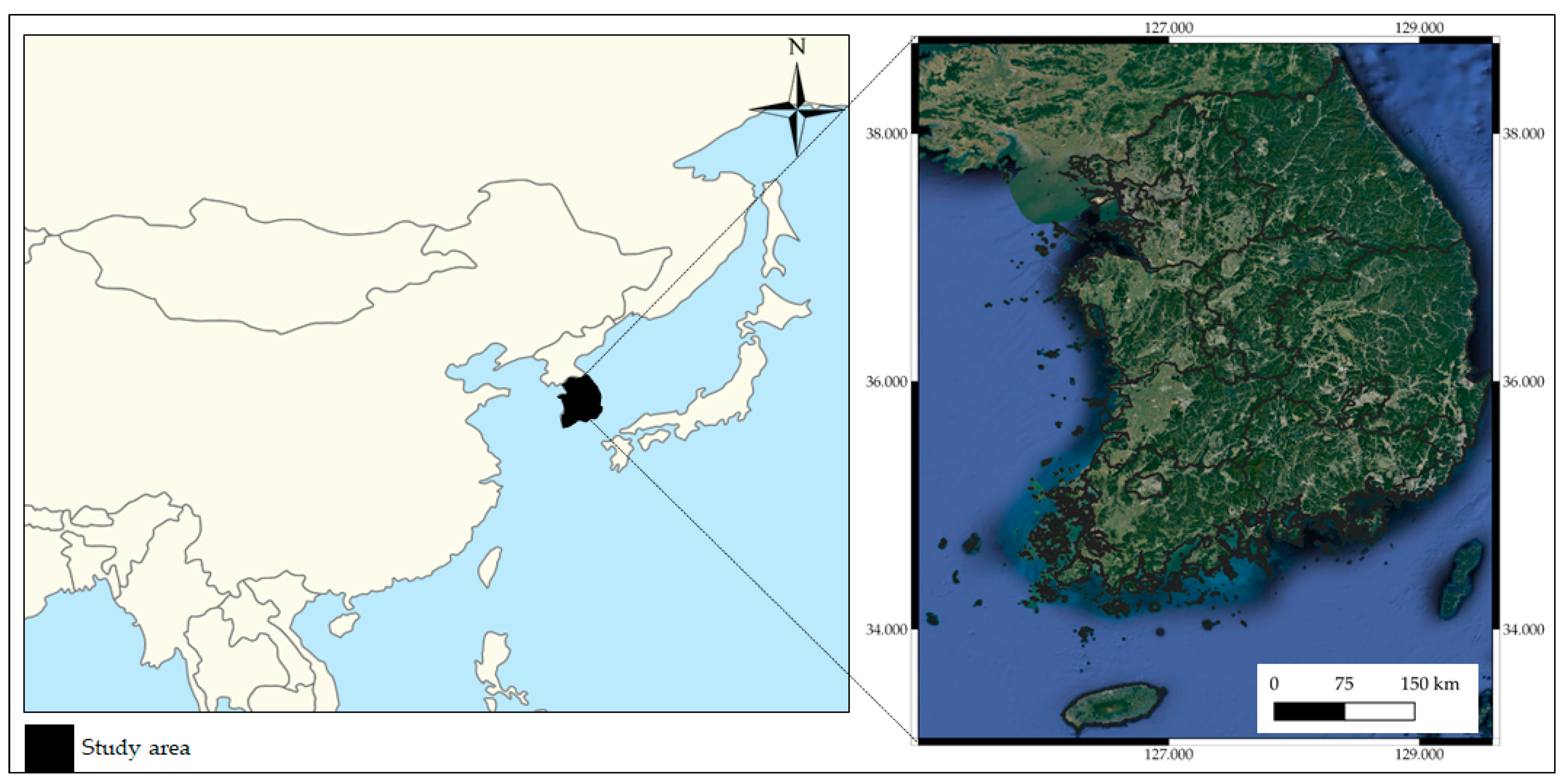
For dataset construction, we considered four least concern (LC) grade species and one endangered (EN) grade species that are considered indicator species for South Korea’s ecosystem, with known different habitat characteristics, as shown in Table 1. The observation data of target species including Hynobius leechii [45], Cyanopica cyanus [46], Platalea minor [47], Hypsipetes amaurotis [48], and Hyla japonica [49] were collected from the GBIF database. Hynobius leechii, known as the Korean salamander, is a species of salamander commonly found on the Korean peninsula which typically inhabits forested hills and wetlands. Cyanopica cyanus mainly lives in Eastern Asia, including China, Korea, and Japan, and lives in coniferous and broad-leaved forests. Platalea minor, known as the Black-faced spoonbill, inhabits the marine coastal zone, the marine intertidal zone, and sea cliffs. Platalea minor is mainly observed in Macau, Hong Kong, Taiwan, Vietnam, and South Korea in winter. Hypsipetes amaurotis typically lives in the Far East of Russia, northeastern China, Japan, and the Korean Peninsula. Hypsipetes amaurotis prefer tropical forests, but can adapt to urban and rural environments. Hyla janoica, called the Japanese tree frog, is widespread in Japan, China, northern Mongolia, the Russian Far East, and Korea. Hypsipetes amaurotis lives in mixed and deciduous broad-leaved forests, wetlands, and river valleys with shrubs. This study is based on the observation data of the target species in South Korea, shown in Figure 2.
Several studies have shown that a sufficient level of species observation data must be obtained for a reasonable SDM performance [50,51]. Therefore, we collected observational data from four popular citizen science databases: GBIF, VertNet, BISON, and Naturing. As discussed above, species observational data in citizen databases are usually spatially biased. Hence, we used the spatial thinning (ST) algorithm in the “spThin” package [52] to alleviate data bias, which returns a refined dataset with the maximum number of presences for a given thinning distance when run for sufficient iterations. ST identifies several new subsets from a set of presences that meet the minimum nearest neighbor distance (NND) constraint. The specific procedure is as follows: (1) A thinning distance x is determined by the user. (2) Pair-wise distances between all presences are calculated. (3) For each presence, the number of presences within distance x is identified. (4) The presence with the highest number of neighboring presences within the NND is determined. (5) One of the presences identified in Step 4 is randomly removed. (6) Steps 3 to 5 are repeated until no presence in the dataset has a nearest neighbor closer than x. In this study, we set the thinning distance to 10 km by considering the target area and the locations of species observation data.
The places where the species were observed were closely related to environmental factors. In particular, land condition, season, and climate have a strong influence on species migration or habitat determination. The climatic condition is generally an important factor in determining the habitat in which a species can live, and the distribution of species can be derived based on this at various spatial resolutions. In addition, most species’ occurrence patterns are highly influenced by temperature and moisture, which are associated with precipitation along the topography. Therefore, it is believed that the distribution of a given species is closely related to topographic and climatic conditions. As all five species have different suitable habitat types, and the sustainable living of each species relies heavily on the land type, we selected the land types as predictors, which elaborately represent the state of the land with a high spatial resolution. As a result, we considered 19 bioclimatic variables from the WorldClim dataset [53] and 14 land cover variables from GlobCover 2009 [54] as input variables. We used 30 arcsec grid bioclimatic variables corresponding to approximately 1 km resolution for small region predictions across South Korea. The GlobCover 2009 dataset was converted from ENVISAT’s medium resolution imaging spectrometer data with approximately 300 m resolution for each spatial grid. We configured all layers’ resolutions to 3000 × 3000 pixels and cropped all layers to the entire South Korean territory, represented by (125.000, 38.083), (129.583, 38.083), (125.000, 33.166), and (129.583, 33.166). Cropped layers were georeferenced based on the World Geodetic System (WGS84). Table 2 summarizes the 33 environmental variables used as input.
We used the variance inflation factor (VIF) to avoid over-fitting,
where is the coefficient of determination for on the other independent variables, and p is the number of independent variables. VIF estimates the impact of the collinearity of on the other independent variables.
VIF is calculated through linear regression, where the regression coefficient ∈ [0,1], with = 0 if there is no multi-collinearity between the input variables, and vice versa. VIF > 10 represents a strong collinearity, which will adversely affect the modeling results. We performed a stepwise selection of environmental variables using VIF. Because VIF values change after each variable is removed, it is not sufficient to use the entire set of environmental variables in the initial comparison. Therefore, we eliminated environmental variables with strong collinearity using a stepwise process to recalculate the remaining input variable’s VIF value after eliminating variables with VIF > 10 [55]. For instance, we calculated the VIF value for each variable, removed the variable with the highest VIF value, and then recalculated all VIF values with a new set of variables until all values were below the threshold.
2.2. Pseudo-Absence and Bootstrap Generation
To generate effective pseudo-absence data, we focused on how to balance the presence and absence data, and where to generate pseudo-absence data. Although PA data should be balanced for effective training, most previous studies have hardly considered this balance when creating datasets. This class imbalance has hindered the predictive performance for ML algorithms and can be alleviated by keeping the PA ratio intermediate [56].
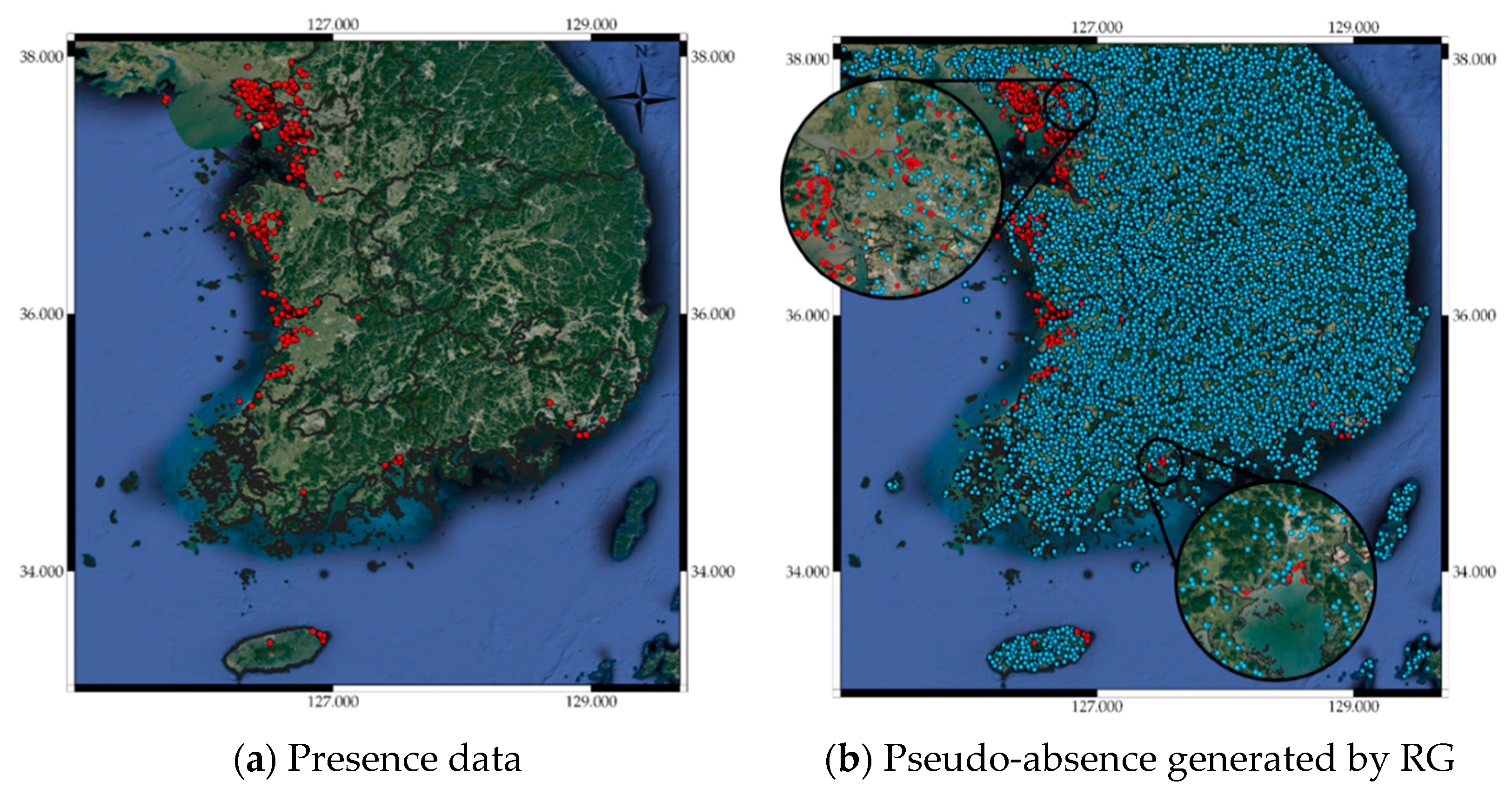
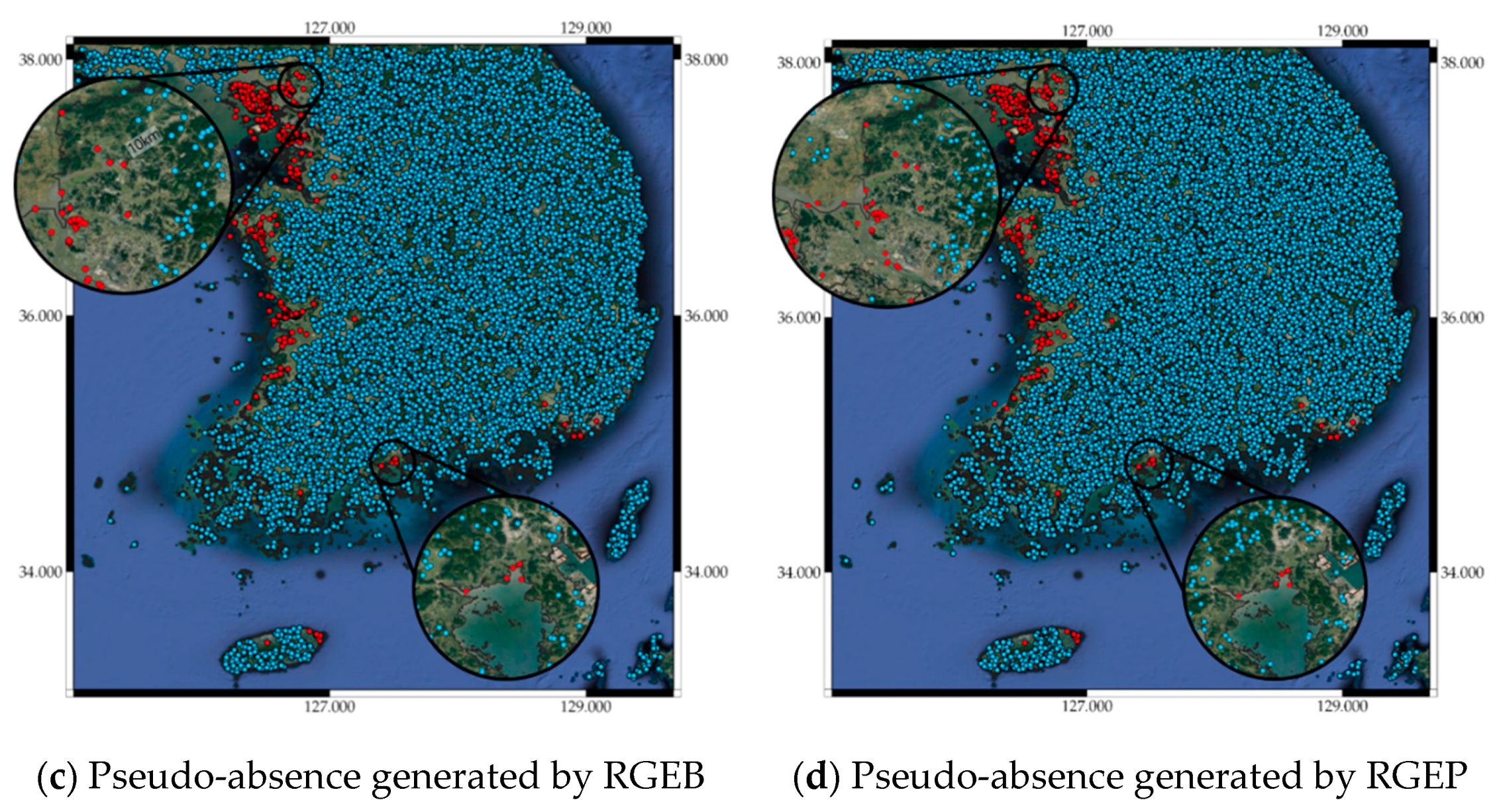
Many SDM studies have shown that the locations implied by generated pseudo-absence data can affect SDM predictive performance [56,57,58]. Randomly generated pseudo-absence data is commonly used to construct SDMs, but this is not always best for all cases [58]. Hence, we investigated random generation (RG), random generation with exclusion buffer (RGEB), and random generation with environmental profiling (RGEP) to find a stable pseudo-absence generation method utilizing the “mopa” package from the R software repository [59]. This package provides designing tools for several factors that influence SDM uncertainty, such as pseudo-absence generation, statistical analysis of selected predictors, and climate projections widely accepted in the species distribution modeling process. RG generates pseudo-absence data randomly across the entire area of interest, whereas RGEB adjusts distances between pseudo-absence data using an exclusion buffer. Several empirical studies have recommended the exclusion buffer = 10 km around each presence location to avoid grids containing both presence and pseudo-absence data [52,53,54]. Therefore, we also adopted a 10 km exclusion buffer when generating random pseudo-absences. RGEP defines the environmental range in which pseudo-absences are sampled. Inappropriate environmental areas can be inferred by one class support vector machines (OCSVMs). An OCSVM, which is one of the unsupervised learning algorithms, is trained only on normal data. In this study, the OCSVM learns the valid boundaries of presences, so any point outside the boundary can be considered a valid site when generating pseudo-absences. Therefore, pseudo-absence locations generated by RGEP are not environmentally similar to presence locations. We have attached the pseudo-absence generation code using the “mopa” package in the Supplementary Materials. Figure 3b–d show pseudo-absence data generated by RG, RGEB, and RGEP, respectively, from the corresponding presence data in Figure 3a.
We subsequently applied bootstrap sampling considering the PA balance. Bootstrap sampling is a resampling method that samples independently with replacement from a sample dataset with the same sample size and performs inferences among these resampled data. Bootstrap sampling reduces biases and strengthens prediction model generalizability [60,61]. Prediction model robustness can be improved by training using bootstraps and combining them, which is known as bootstrap aggregating or bagging. Many studies have shown advantages from bagging [60,61,62]. We generated 10 times more pseudo-absence data than presence data using three pseudo-absence data generating methods, as shown in Figure 3b–d, and selected the same number of pseudo-absence data points as the number of presences, allowing for resampling with replacement. Bootstrap samples were generated using the “boot” R package [62]. We included the code for generating bootstraps using the “boot” package in the Supplementary Materials. Thus, we obtained N bootstrap samples suitable for training machine learning models.
2.3. Ensemble Approach for Model Construction
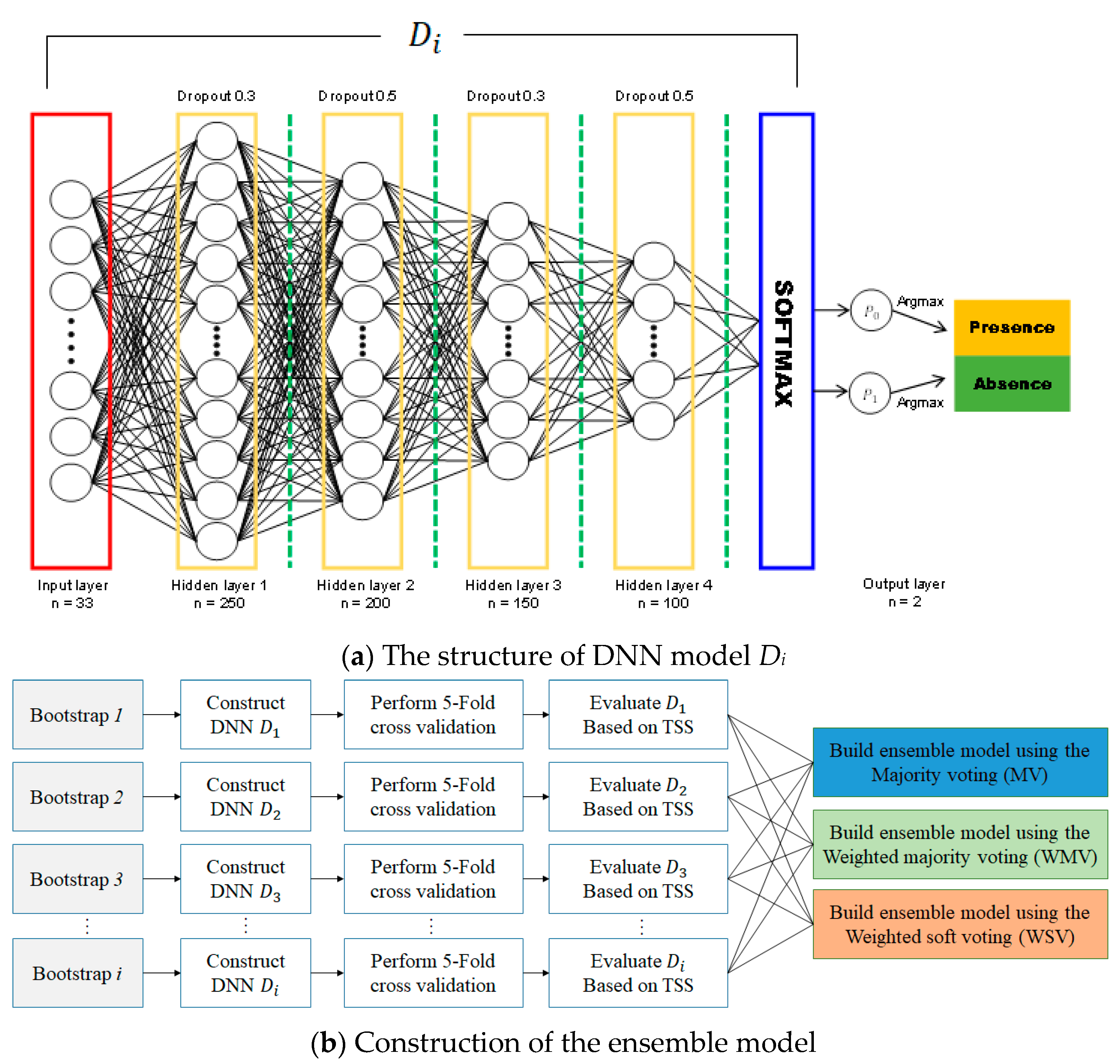
Recent deep learning developments have enabled new SDM possibilities. Since DNN-based SDMs have already shown better performance than various traditional models [38,63,64], we combined multiple DNNs constructed using bootstraps to maximize prediction performance, which is known as ensemble modeling. Figure 4a shows the proposed DNN model structure for species distribution predictions. The model comprises three layers, similar to typical DNN models, with the input layer receiving environmental variables corresponding to PA locations. Hidden layers perform a weighted summation of the inputs followed by a non-linear transformation. The output layer produces final predictions derived from softmax, which transforms all network activations into a series of values that can be interpreted as probabilities. The sum of the probabilities of all classes must amount to 1.
To optimize the DNN, we calculated optimal hyper-parameters using grid search [59,60], which includes an infinite number of grid search iterations, five cross-validations, four hidden layers (with 250, 200, 150, and 100 neurons each), a batch size of 75, a learning rate of 0.001, and 10,000 epochs with early stopping. Other hyper-parameters are L2 regularization, to prevent the overfitting of DNN, adaptive moment estimation (Adam) optimization, to update the weights of the DNN model iteratively based on training data, the rectified linear unit (ReLU) activation function, to overcome the vanishing gradient problem, and the cross entropy error loss function, to calculate the difference between two probability distributions. These hyperparameters were determined empirically because they provided the best performance during cross-validation.
To initialize the weights for neuron inputs, we used the he-normal (HE) initialization. Each DNN model was trained until the optimization process was done. Our trained DNN model was used to produce the probability of presence and absence for a species. The more suitable the regions in the study area for a particular species’ habitat, the closer the probability is to 1, and vice versa.
Subsequently, we built an ensemble model based on the trained models to improve generality and predictive performance. The ensemble technique reduces over-fitting and provides a better predictive performance than a single model, and has been widely used for ecological modeling [63,64]. Figure 4b presents the schematic of the ensemble model construction process. Each DNN model Di trained by bootstrap sample i performs a five-fold cross-validation. Then, each Di is evaluated by the true skill statistic (TSS) value that is used as the weight in ensemble modeling. The trained DNNs, which can be regarded as sub-models, were combined using majority (MV), weighted majority (WMV), and weighted soft (WSV) voting schemes. MV is a simple and effective combination method to solve classification problems, and we denoted class label outputs for sub-model as c-dimensional binary vectors,
where i = 1, …, N; = 1 or 0 depending on whether sub-model correctly chooses or not; and N is the number of sub-models. The majority voting rule gives an ensemble decision for class prediction.
WMV assigns a weight to each sub-model and aggregates their prediction results. The underlying concept is that an outstanding sub-model will have a relatively high weight, ≈ 1, whereas weaker sub-models will have a relatively lower weighted value, ≈ 0. Weight can be assigned to the ith sub-model using the normalized true skill statistic for each sub-model, i.e., the average from a five-fold cross-validation. TSS is a reliable evaluation metric for SDM performance. Hence, we used a normalized TSS for the weight,
with the final prediction:
Assuming the ensemble model is well calibrated for predicting species distribution, a weighted soft voting scheme can be applied to combine the sub-models. Class labels are determined based on the predicted probability p for each classifier,
2.4. Evaluation Approach
Five evaluation metrics were employed to assess SDM performance: area under the curve (AUC), sensitivity, specificity, kappa statistic K, and true skill statistic TSS, which have been widely used for ecological studies [56,57,58]. Table 3 shows the confusion matrix summarizing correspondence between observations and predictions in terms of true positives (TP), true negatives (TN), false positives (FP), and false negatives (FN). We used 0.5 as the threshold to calculate TP, TN, FP, and FN, which are widely used in SDM evaluation.
AUC represents how well the model discriminates presence from pseudo-absence data, where AUC closer to 1 implies better discrimination performance. Sensitivity, also called hit rate, measures how well the model infers presence data,
Specificity indicates how well a model can infer absence data,
Kappa statistic K measures the extent to which the agreement between observed and predicted is higher than that expected by chance alone,
Therefore, Κ can alleviate overestimating accuracy. TSS is defined from the standard confusion matrix components and represents matches and mismatches between observation and predictions,
TSS is often used as an alternative to AUC, and is probably the best model performance summary. Table 4 shows the evaluation criteria for AUC, Κ, and TSS metrics to evaluate SDM performance.
3. Experimental Results
3.1. Experimental Setting
The prediction performance for the proposed model was compared with the current best practice SDMs on several public datasets. Datasets were balanced using three data generation methods to solve the bias problem for most observation datasets, and their effectiveness was evaluated. Table 5 shows that the comparison SDMs included classification tree analysis (CTA), shallow neural network (SNN), flexible discriminant analysis (FDA), and multivariate adaptive regression splines (MARS), GLM, GBM, RF, SRE, and MAXENT. All models were implemented using “BIOMOD2” in R, a popular tool for ecological modeling [61]. Training strategies and selected parameters are also shown in Table 5. Three prediction models were considered depending on the ensemble method: MV-based DNNs for the ensemble (MV-EDNN), WMV-based DNNs for the ensemble (WMV-EDNN), and WSV-based DNNs for the ensemble (WSV-EDNN). These were built using the Scikit-learn Python package [65], with 80% of the target species observations as training and 20% as test sets. We used the “BIOMOD_Modeling” function in the “BIOMOD2” R software package to evaluate and calibrate the range of species distribution models techniques run over a given species [64]. In the Supplementary Materials, we included the calibration results of all prediction model and target species, as shown in Figures S1–S5. Our calibration process was performed with an 80% random subpart of the given species’ presence-absence dataset. To validate the prediction models, we used a five-fold cross-validation with five-time evaluation runs and recorded their average results. We included our experimental code in the Supplementary Materials.
3.2. Pseudo-Absence Generation Strategy Effects
This section compares various SDM performances under three pseudo-absence generation strategies. Although RG is popularly used to generate pseudo-absence data for SDM, we also tested RGEB and RGEP to find the best method to improve predictive power. We set the presence and pseudo-absence ratio for the training and test sets to 0.5, with 80% and 20% dataset split, respectively. Table 6, Table 7 and Table 8 show average estimation results for the three generation methods for all target species.
Most SDMs showed a significant prediction performance improvement under RGEB and RGEP compared with RG. Although RG is the simplest and most common method to generate pseudo-absences, RGEB and RGEP provided a better predictive ability improvement, resulting in more reliable prediction maps for species distribution.
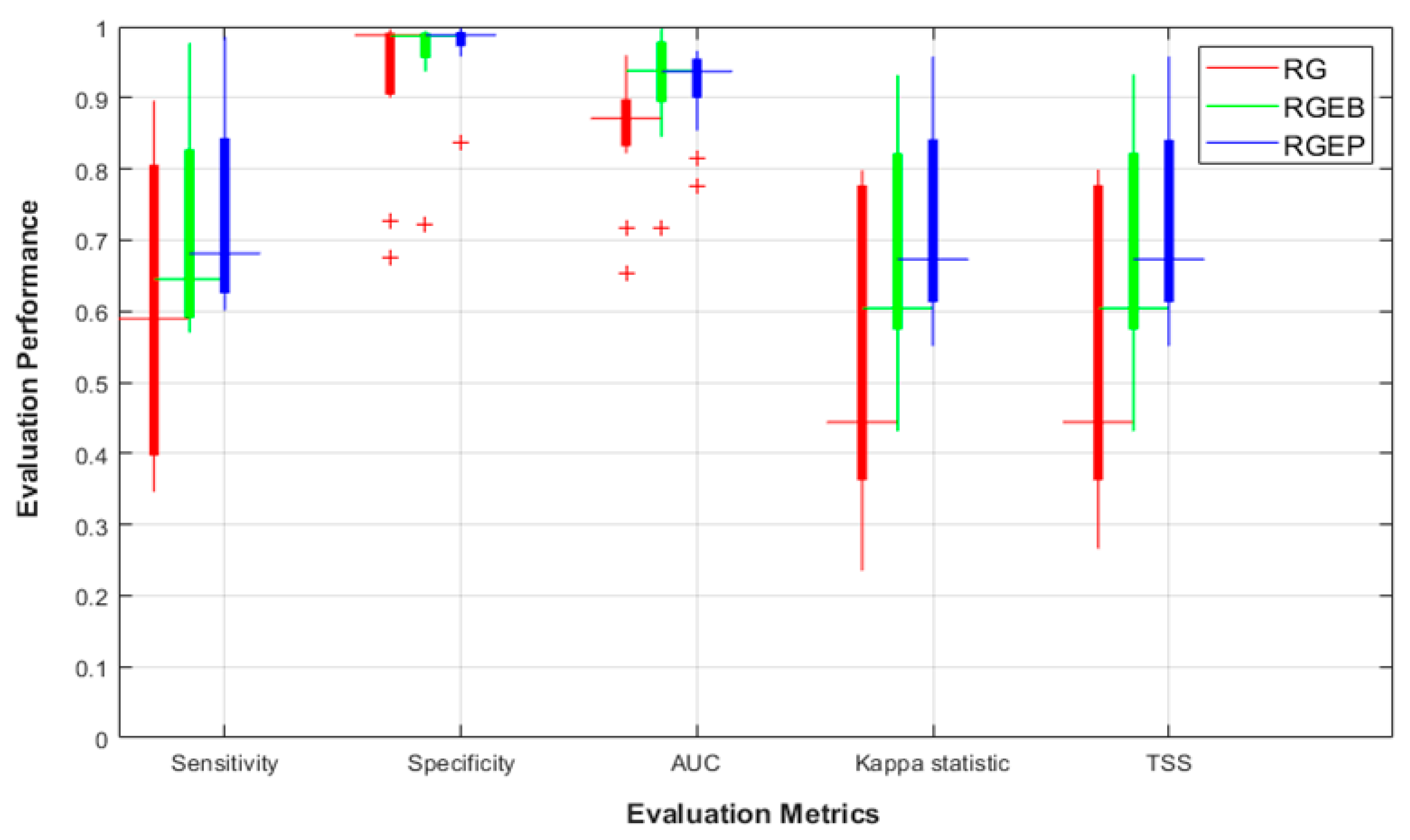
Figure 5 compares the prediction performance for the three generation methods using a five-fold cross validation. RGEP provided a better performance and variance for all metrics compared with RG and RGEB, with mean sensitivity = 0.681, 0.589, and 0.645, respectively. In the case of specificity, RGEB and RGEP methods reduced false absence predictions, i.e., narrower specificity box ranges than RG. Considering AUC, Κ, and TSS, RGEB and RGEP methods provided a better prediction ability for most SDMs than RG. Thus, RGEP was the most effective overall method in terms of performance improvement.
3.3. SDM Stability for Unbalanced Datasets
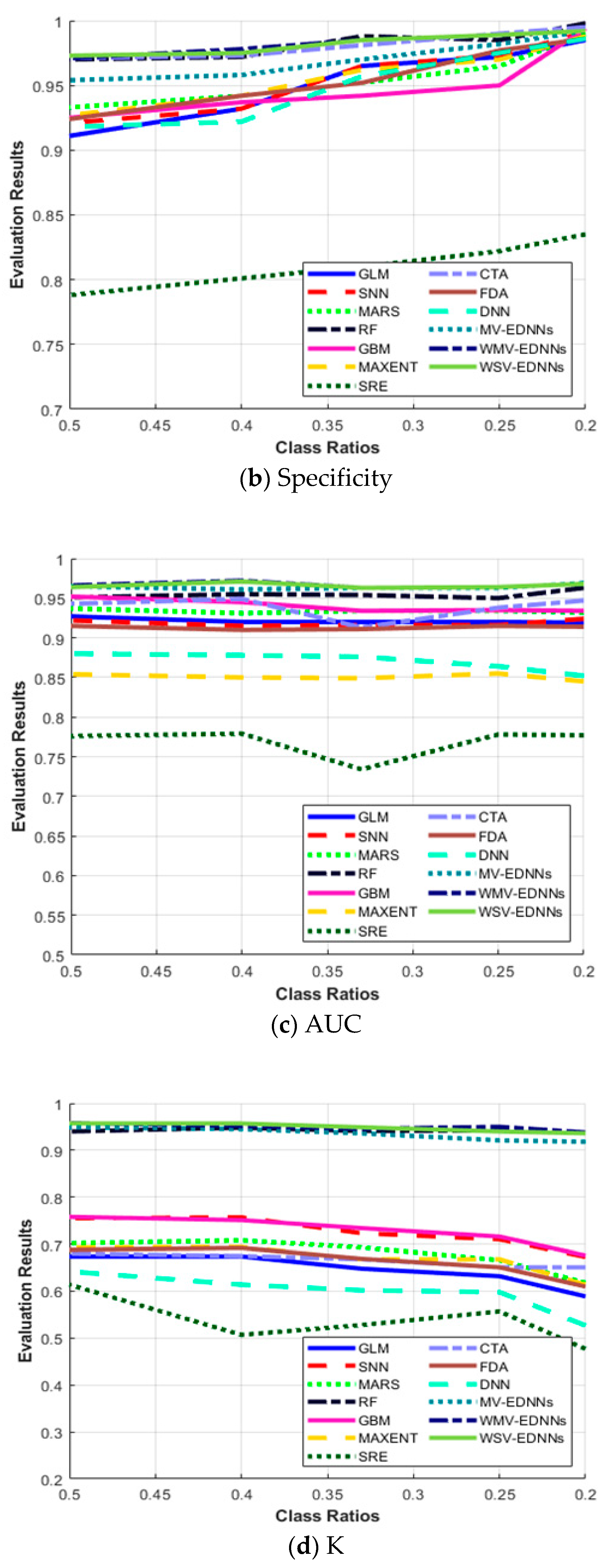
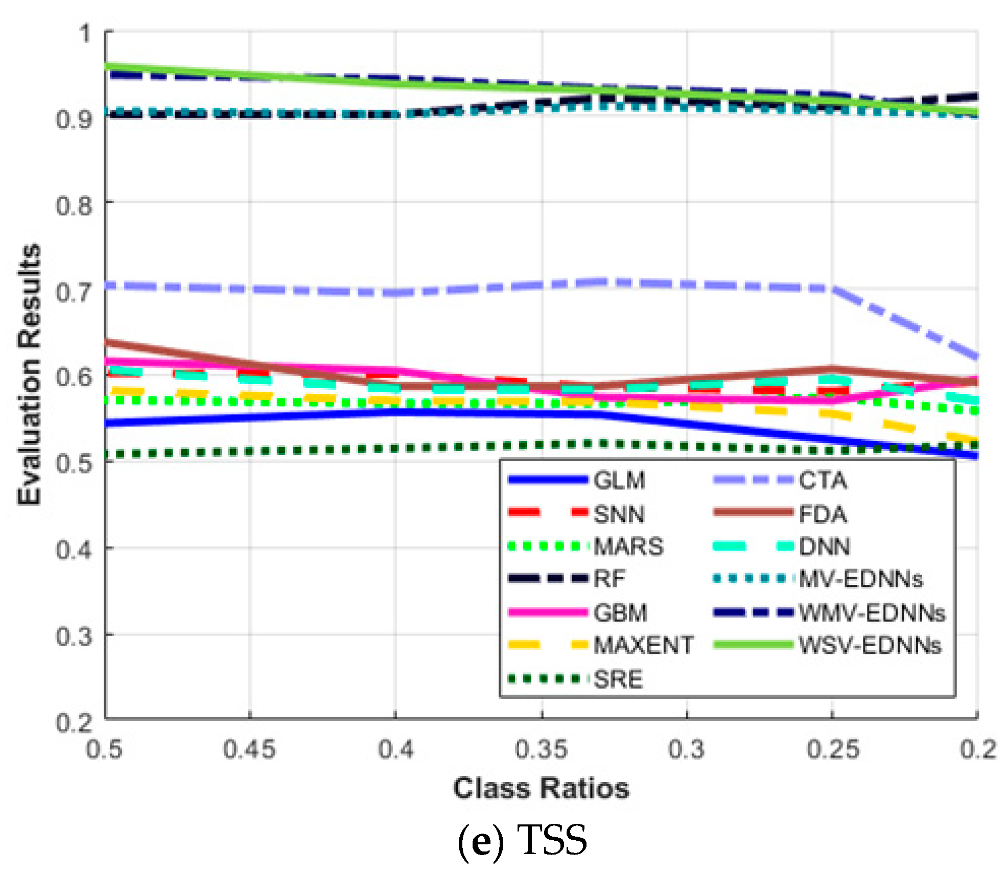
This section investigates the SDM prediction stability for different presence to pseudo-absence ratios. Training sets were organized by randomly selecting presences and absences from the full dataset excluding test data, where and represent dataset size and class ratio, respectively. We used as test presence and absence. Table 9 shows the evaluation results for SDM target species with respect to using a five-fold cross-validation and mean evaluation metrics.
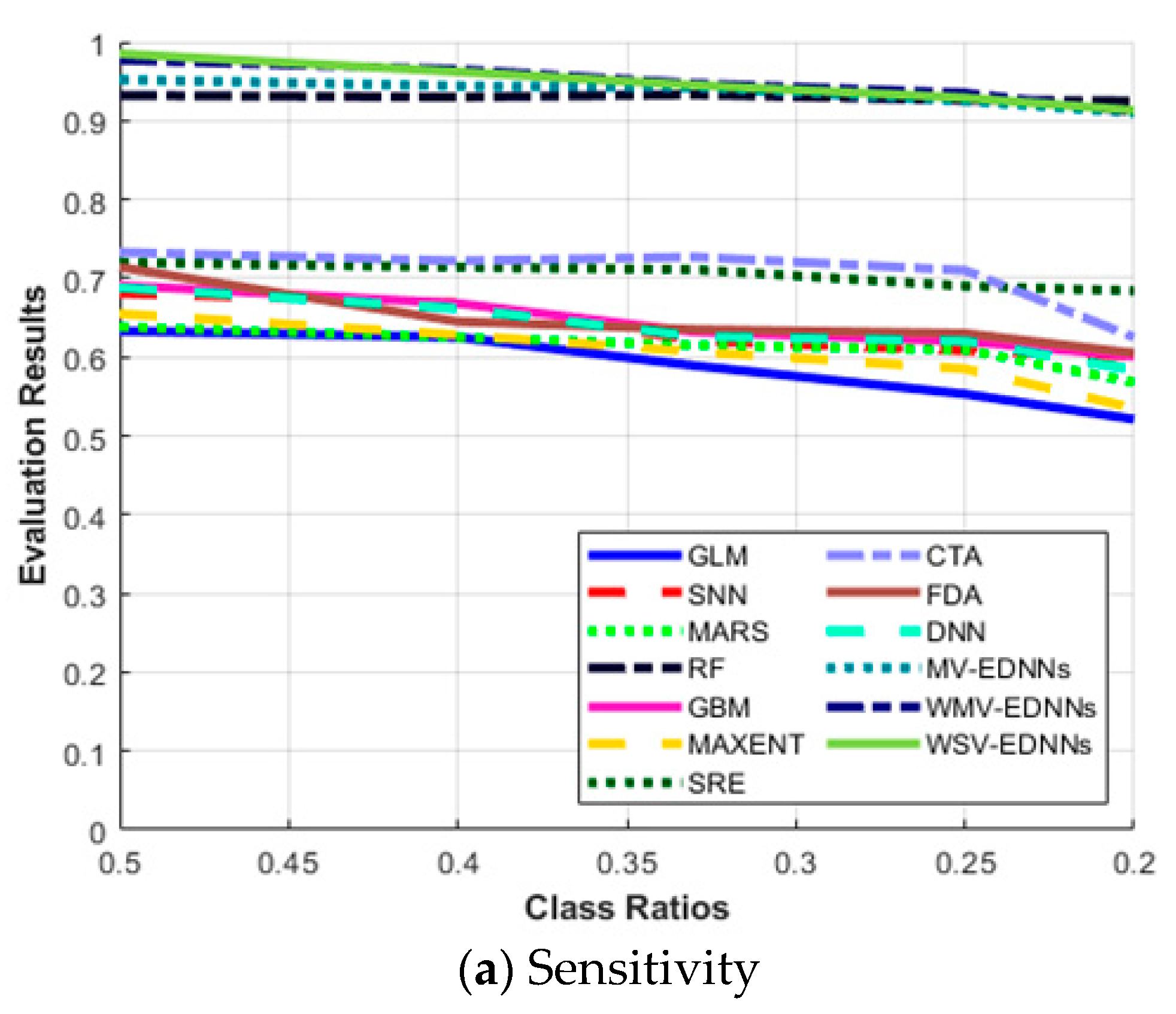
Figure 6a shows that the highest results for all the evaluation metrics were achieved for balanced class ratio, i.e., π = 0.5. The average sensitivity for most SDMs decreased as π decreased, and vice versa for specificity. The three proposed models, MV-EDNNs, WMV-EDNNs, and WSV-EDNNs, achieved the best overall prediction performance for 0.2 < π < 0.5. The bagging-based SDMs’ (the three proposed and RF models) performance reduced as π decreased from 0.5 to 0.2. Sensitivity decreased considerably, except for bagging-based SDMs, as π changed from 0.5 to 0.2, whereas specificity showed a relatively large increase for GLM, CTA, SNN, GBM, and MAXENT SDMs (Figure 6b).
Figure 6c–e show that although GLM, SNN, MARS, GBM, MAXENT, SRE, CTA, and DNN achieved a relatively high AUC, they had a relatively low Κ and TSS performance. Thus, these SDMs were good at predicting pseudo-absences, but were not good at predicting presences. AUC has been a standard method to assess predictive distribution model accuracy. However, it is highly affected by a well-predicted absence rate. All SDMs except bagging-based SDMs exhibited significantly decreased Κ as π decreased to 0.2, whereas bagging-based SDMs exhibited very little Κ reduction as π decreased. Thus, bagging-based SDMs outperformed typical SDMs as the species datasets became more unbalanced.
3.4. Impact of the Ensemble Size
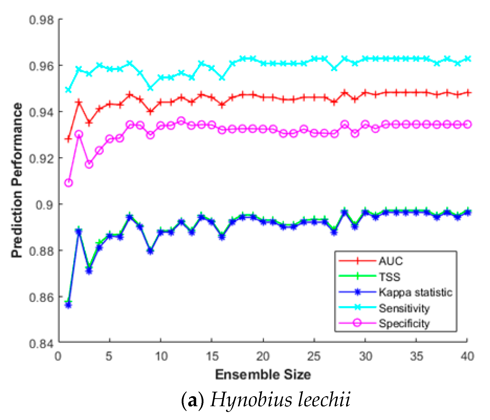
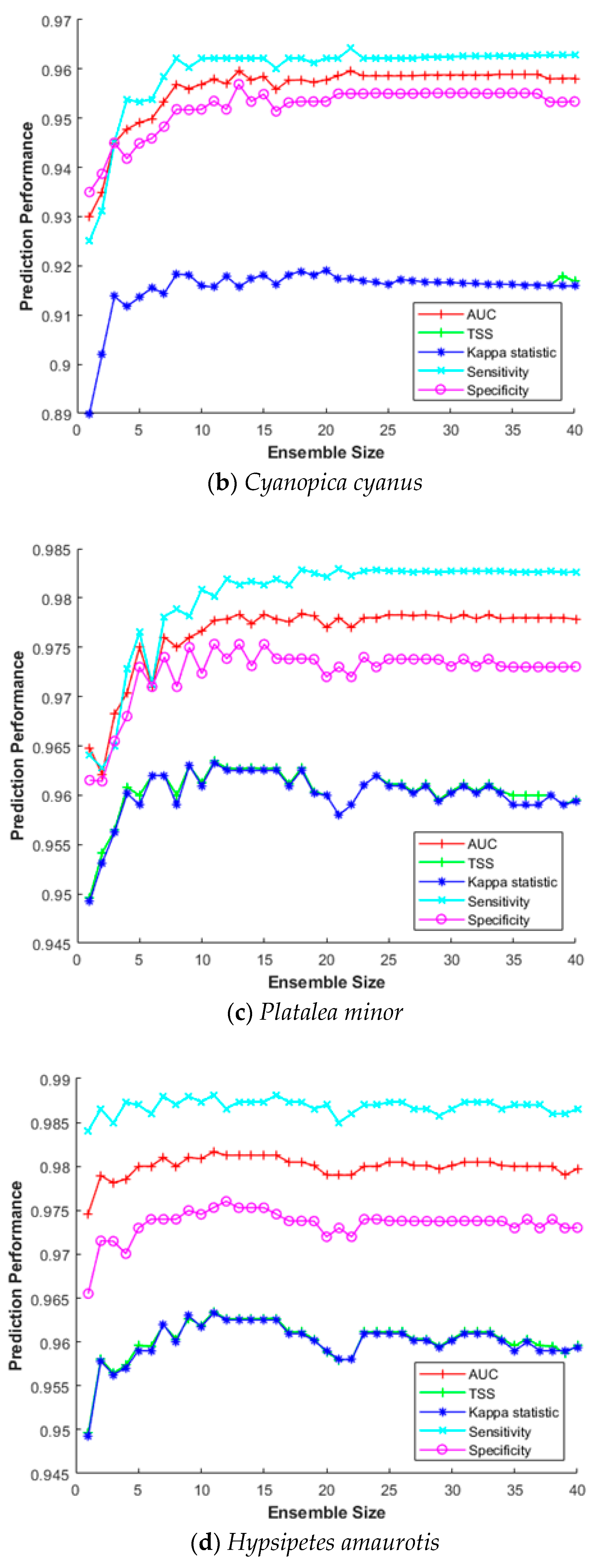
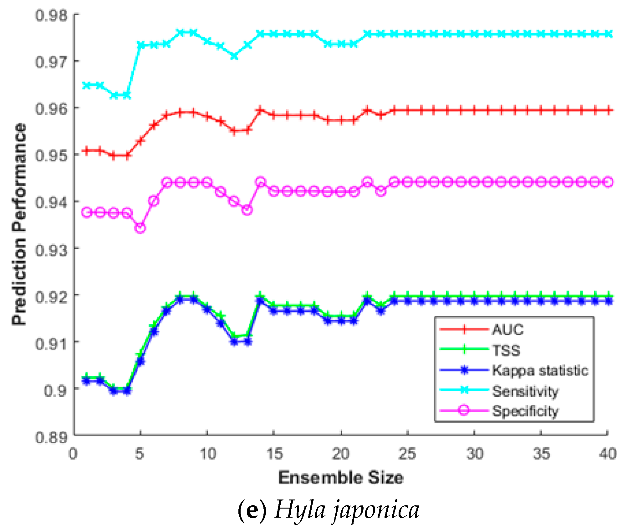
This section investigates the impact of the ensemble size for constructing SDM efficiently. The ensemble size refers to how many bootstrap trained sub-models were combined to build the final prediction model. Combining multiple sub-models does not always improve prediction performance; hence, it is important to find optimal combinations in terms of processing time and cost. Therefore, we measured sensitivity, specificity, AUC, Κ, and TSS for increasing the ensemble size from 2 to 40 for five species (Hynobius leechii, Cyanopica cyanus, Platalea minor, Hypsipetes amaurotis, and Hyla japonica). As above, we used a five-fold cross-validation for MV-EDNN, WMV-EDNN, and WSV-EDNN, and average evaluation scores to assess the impact of the ensemble size.
Figure 7 shows that although there is some difference depending on the species, performance improved as the ensemble size increased up to a certain point, with relatively little further improvement beyond that, e.g., maximum Κ and TSS = 0.891 and 0.890, respectively, for Hynobius leechii when ensemble size = 27 (Figure 7a). Thus, an appropriate ensemble size can provide a better performance than individual models in most cases.
3.5. Case Study
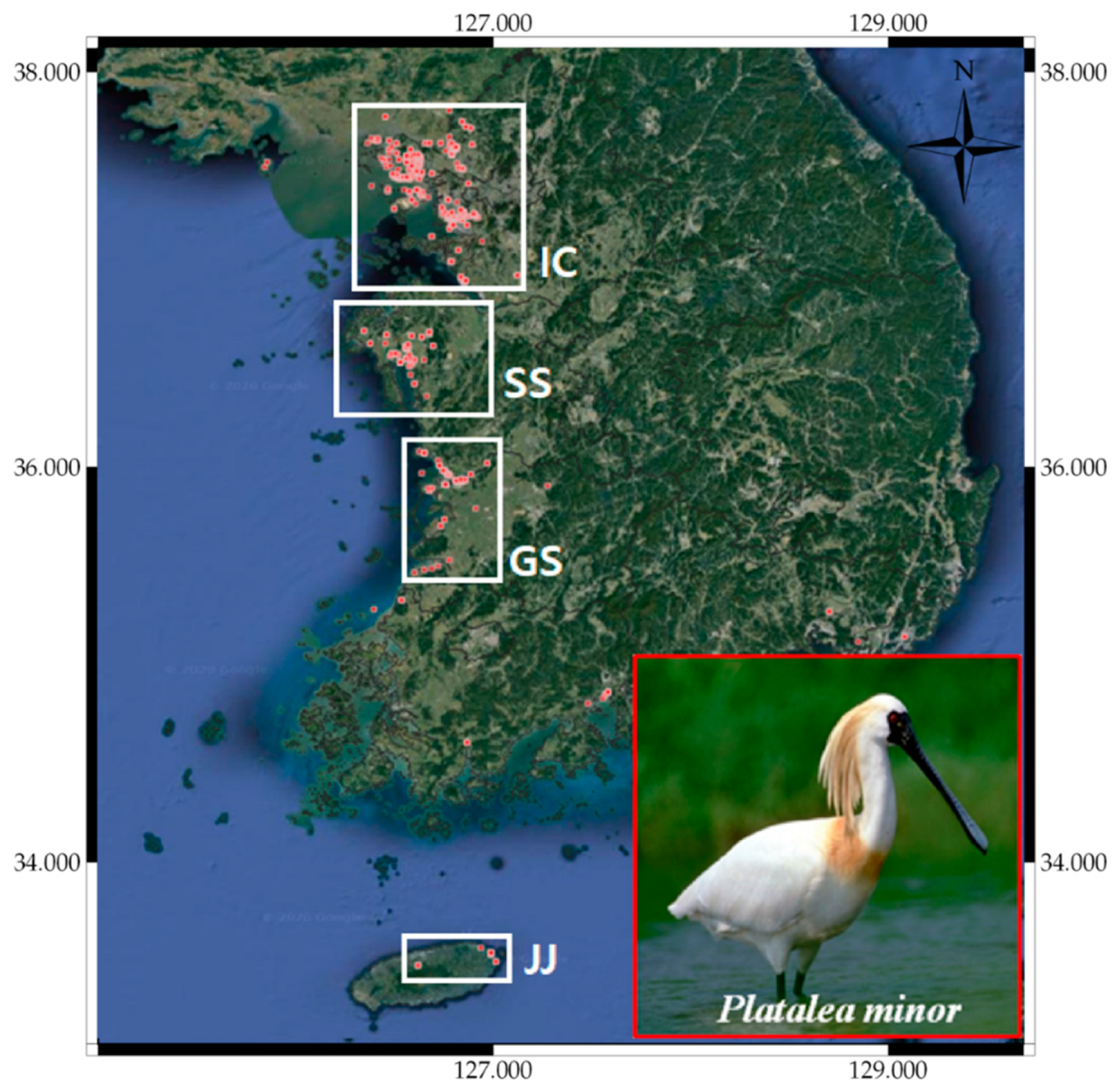
We selected the Platalea minor’s distribution to verify the prediction outcomes. Platalea minor, also known as black-faced spoonbill, lives mainly in Korea, Hong Kong, and Taiwan and is designated as “endangered” in the IUCN red-list (see Table 1). The species has also been designated as a Natural Monument (No. 205-1) by the Cultural Heritage Administration of Korea and is classified as endangered species Ⅰ by the Ministry of Environment of Korea [66]. This species is the rarest of those considered here, with less than 2700 individuals observed in Hong Kong and Taiwan during the winter season. Platalea minor was mainly observed on the west coast of the Korean Peninsula from June to August, which is closely related to their breeding season [66,67], and suitable habitats include marine coastal zones, estuaries, tidal flats, and fishponds. The bird is as tactile feeder, walking slowly and stirring the water with its beak to catch its prey. Therefore, tidal flats and marine coastal zones provide suitable foraging areas, combining shallow and turbid water. Platalea minor collect sticks, etc., from nearby trees or pastures to build their nests, and the distribution of observation data reflected their foraging and breeding habitats well [66].
Figure 8 shows that the observations of Platalea minor in South Korea were more prevalent in and around the Incheon Bay (IC), Seosan Bay (SS), Gunsan Bay (GS), and Jeju Coastal (JJ) regions. The endangered species has a limited habitat and hence a relatively narrow range of observations. We used observations from IC, SS, and JJ as the training set and observations from GS as the test set, with RGEP pseudo-absence generation.
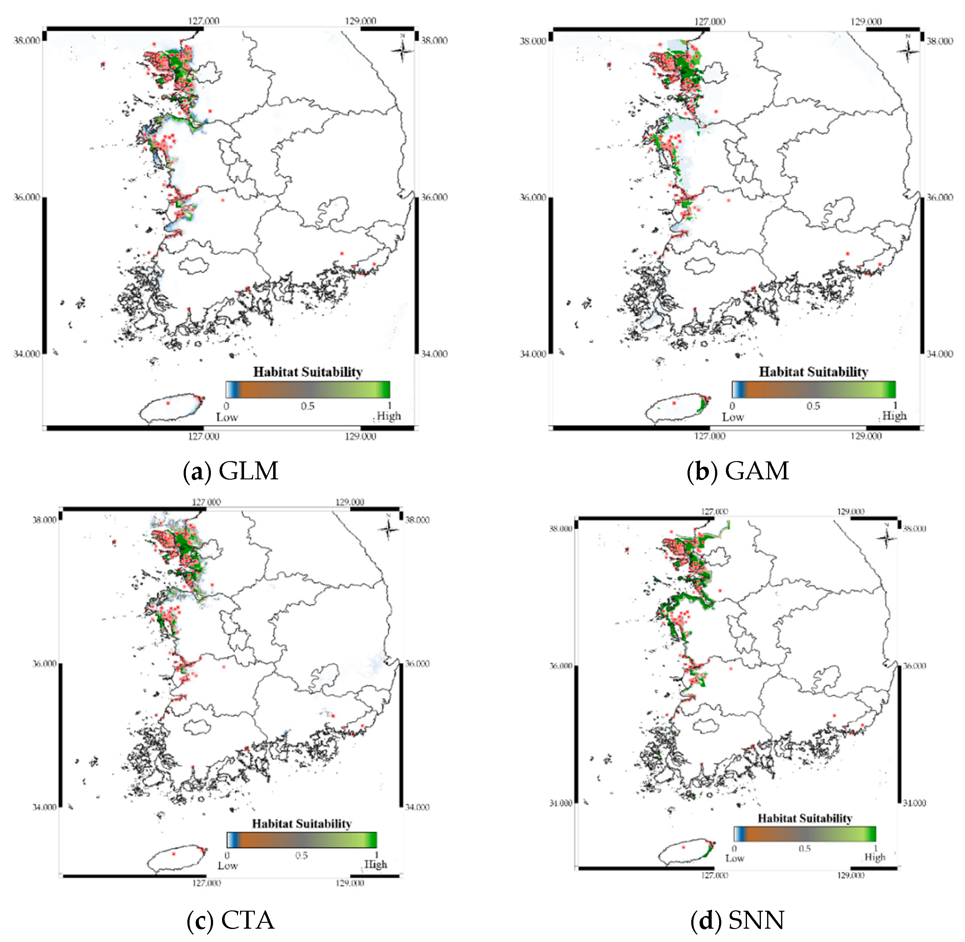
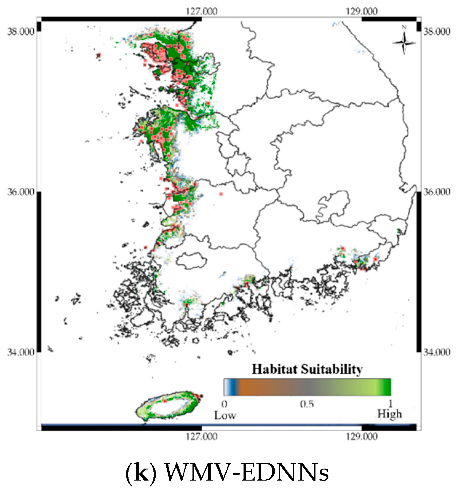
Figure 9 shows the distribution prediction results for Platalea minor. WMV-EDNNs achieved the best performance (Sensitivity = 0.976, TSS = 0.958) compared with other SDMs (Sensitivity = 0.699 ± 0.108, TSS = 0.842 ± 0.094). Although the performance of RF was slightly poorer than that of WMV-EDNN, it exhibited excellent prediction performance (Sensitivity = 0.932, TSS = 0.931), considering it employed bootstrapping. Thus, when using observation data with spatial biases collected in a narrow range (e.g., observation data of Platalea minor), typical SDMs showed a relatively lower prediction performance than bootstrap-based approaches.
4. Discussion
The key to maintaining biodiversity is to preserve the habitats of endangered or threatened species, or to find alternative habitats that are more likely to survive. According to the IUCN report, it is estimated that as many as one million species are predicted to be on the verge of extinction over the next decades. Therefore, a practical countermeasure with a high probability of success is urgently needed. In this study, we showed that well-trained DNNs and their ensemble have achieved better prediction performance than typical machine learning methods such as GLM, GAM, CTA, SNN, FDA, MARS, RF, SRE, and MAXENT, which are widely used for species distribution prediction. Our proposed model can be used to find alternative habitats for endangered species, and can be regarded as a long-term species conservation strategy.
In general, species’ presence and absence data are needed to build an SDM. If reliable real absence data are not available, one alternative to obtaining absence data is to generate pseudo-absences. Several studies have suggested that pseudo-absence data should be confined to locations that are clearly not suitable for species habitats [56,68]. However, for large study areas, it takes a very long time to individually identify such sites for each species, and it is much more difficult to verify the ecological aspect. Therefore, we believe that an effective pseudo-absence generation strategy is required to construct a practical SDM. By implementing RG, RGEB, and RGEP, we have found that the RGEP method is the best pseudo-absence generation method when true-absence data are not available. In the modeling process, the bootstrapping approach is robust to changes in prevalence, so this approach is worth considering if the acquisition of presence data is limited. Finally, we used crowdsourced datasets to obtain data necessary for our SDM construction, which can cause some biases in the observation data and prediction results. As far as we know, this is an inevitable limitation when using crowdsourced data. In future studies, we plan to develop standard procedures for SDM that include the reduction of observational bias, the selection of the best environmental variables, and self-optimization.
5. Conclusions
Many ecological models have been devised for various purposes, including biodiversity conservation, rare species protection, and habitat suitability assessment. However, current SDMs suffer from critical limitations, such as data imbalance and spatial bias. Therefore, we proposed a bootstrap aggregating (bagging) deep neural network (DNN) ensemble species distribution model. Specifically, we collected sufficient observations from various citizen science databases, generated bootstraps to train DNNs, and finally combined the DNNs using MV, WMV, and WSV techniques to provide stable ensemble prediction models.
We compared the models with other SDMs to verify the proposed approach’s effectiveness using five evaluation metrics. WMV-EDNNs achieved a stronger and more stable prediction performance than the other two ensemble models and existing SDMs for diverse scenarios.
Platalea minor species distribution was visualized using map overlays to show prediction results intuitively. Although Platalea minor observations had a spatially biased distribution in the dataset, WMV-EDNN models achieved a superior predictive performance compared with current SDMs. Thus, bagging-ensemble-based SDMs achieved robustness prediction performance, although the observation dataset was spatially biased and unbalanced.
Supplementary Materials
The following are available online at https://0-www-mdpi-com.brum.beds.ac.uk/article/10.3390/rs13081495/s1, Table S1: Selected environmental parameters using stepwise VIF algorithm runs (VIF < 10), Figure S1: Calibration results for Hynobius leechii distribution, Figure S2: Calibration results for Cyanopica cyanus distribution, Figure S3: Calibration results for Platalea minor distribution, Figure S4: Calibration results for Hypsipetes amaurotis distribution, Figure S5: Calibration results for Hyla japonica distribution.
Author Contributions
Conceptualization, J.R.; methodology, J.R. and Y.C.; software, J.R. and Y.C.; validation, J.R. and Y.C.; investigation, Y.C.; data curation, J.R. and Y.C.; visualization, J.R. and Y.C.; writing—original draft preparation, J.R.; writing—review and editing, E.H.; supervision, E.H.; and project administration, E.H. All authors have read and agreed to the published version of the manuscript.
Funding
This research was supported by a government-wide R&D Fund project for infectious disease research (GFID), Republic of Korea (grant number: HG19C0682).
Institutional Review Board Statement
Not applicable.
Informed Consent Statement
Not applicable.
Conflicts of Interest
The authors declare no conflict of interest.
References
- Tscharntke, T.; Clough, Y.; Wanger, T.C.; Jackson, L.; Motzke, I.; Perfecto, I.; Vandermeer, J.; Whitbread, A. Global food security, biodiversity conservation and the future of agricultural intensification. Biol. Conserv. 2012, 151, 53–59. [Google Scholar] [CrossRef]
- Potts, S.G.; Biesmeijer, J.C.; Kremen, C.; Neumann, P.; Schweiger, O.; Kunin, W.E. Global pollinator declines: Trends, impacts and drivers. Trends Ecol. Evol. 2010, 25, 345–353. [Google Scholar] [CrossRef] [PubMed]
- Collins, J.P.; Storfer, A. Global amphibian declines: Sorting the hypotheses. Divers. Distrib. 2003, 9, 89–98. [Google Scholar] [CrossRef]
- Wood, P.M. Biodiversity as the source of biological resources: A new look at biodiversity values. Environ. Values 1997, 6, 251–268. [Google Scholar] [CrossRef]
- Simpson, R.D.; Sedjo, R.A.; Reid, J.W. Valuing biodiversity for use in pharmaceutical research. J. Political Econ. 1996, 104, 163–185. [Google Scholar] [CrossRef]
- Butchart, S.H.; Walpole, M.; Collen, B.; Van Strien, A.; Scharlemann, J.P.; Almond, R.E.; Baillie, J.E.; Bomhard, B.; Brown, C.; Bruno, J.; et al. Global biodiversity: Indicators of recent declines. Science 2010, 328, 1164–1168. [Google Scholar] [CrossRef]
- Almond, R.; Grooten, M.; Peterson, T. Living Planet Report 2020—Bending the Curve of Biodiversity Loss; World Wildlife Fund: Gland, Switzerland, 2020. [Google Scholar]
- Wilcove, D.S.; Rothstein, D.; Dubow, J.; Phillips, A.; Losos, E. Quantifying threats to imperiled species in the United States. BioScience 1998, 48, 607–615. [Google Scholar] [CrossRef] [Green Version]
- Langpap, C.; Kerkvliet, J. Endangered species conservation on private land: Assessing the effectiveness of habitat conservation plans. J. Environ. Econ. Manag. 2012, 64, 1–15. [Google Scholar] [CrossRef] [Green Version]
- Bonnie, R. Endangered species mitigation banking: Promoting recovery through habitat conservation planning under the Endangered Species Act. Sci. Total Environ. 1999, 240, 11–19. [Google Scholar] [CrossRef]
- Elith, J. Quantitative Methods for Modeling Species Habitat: Comparative Performance and an Application to Australian Plants; Springer: New York, NY, USA, 2006; pp. 39–58. [Google Scholar]
- Braunisch, V.; Suchant, R. A model for evaluating the ‘habitat potential’ of a landscape for capercaillie Tetrao urogallus: A tool for conservation planning. Wildl. Biol. 2007, 13, 21–33. [Google Scholar] [CrossRef] [Green Version]
- Wu, X.B.; Smeins, F.E. Multiple-scale habitat modeling approach for rare plant conservation. Landsc. Urban Plan. 2000, 51, 11–28. [Google Scholar] [CrossRef]
- Poulos, H.M.; Chernoff, B.; Fuller, P.L.; Butman, D. Ensemble forecasting of potential habitat for three invasive fishes. Aquat. Invasions 2012, 7, 59–72. [Google Scholar] [CrossRef]
- Brown, J.L. SDMtoolbox: A python-based GIS toolkit for landscape genetic, biogeographic and species distribution model analyses. Methods Ecol. Evol. 2014, 5, 694–700. [Google Scholar] [CrossRef]
- Václavík, T.; Meentemeyer, R.K. Equilibrium or not? Modelling potential distribution of invasive species in different stages of invasion. Divers. Distrib. 2011, 18, 73–83. [Google Scholar] [CrossRef]
- Robinson, T.P.; van Klinken, R.D.; Metternicht, G. Comparison of alternative strategies for invasive species distribution modeling. Ecol. Model. 2010, 221, 2261–2269. [Google Scholar] [CrossRef] [Green Version]
- Raes, N.; ter Steege, H. A null-model for significance testing of presence-only species distribution models. Ecography 2007, 30, 727–736. [Google Scholar] [CrossRef]
- Zaniewski, A.E.; Lehmann, A.; Overton, J.M. Predicting species spatial distributions using presence-only data: A case study of native New Zealand ferns. Ecol. Model. 2002, 157, 261–280. [Google Scholar] [CrossRef]
- Rebelo, H.; Jones, G. Ground validation of presence-only modelling with rare species: A case study on barbastelles Barbastella barbastellus (Chiroptera: Vespertilionidae). J. Appl. Ecol. 2010, 47, 410–420. [Google Scholar] [CrossRef]
- Aarts, G.; Fieberg, J.; Matthiopoulos, J. Comparative interpretation of count, presence-absence and point methods for species distribution models. Methods Ecol. Evol. 2012, 3, 177–187. [Google Scholar] [CrossRef]
- Elith, J.; Graham, C.H. Do they? How do they? WHY do they differ? On finding reasons for differing performances of species distribution models. Ecography 2009, 32, 66–77. [Google Scholar] [CrossRef]
- Manel, S.; Williams, H.C.; Ormerod, S.J. Evaluating presence-absence models in ecology: The need to account for prevalence. J. Appl. Ecol. 2001, 38, 921–931. [Google Scholar] [CrossRef]
- Duan, R.-Y.; Kong, X.-Q.; Huang, M.-Y.; Fan, W.-Y.; Wang, Z.-G. The predictive performance and stability of six species distribution models. PLoS ONE 2014, 9, e112764. [Google Scholar] [CrossRef] [PubMed] [Green Version]
- Munguía, M.; Rahbek, C.; Rangel, T.F.; Diniz-Filho, J.A.F.; Araújo, M.B. Equilibrium of global amphibian species distributions with climate. PLoS ONE 2012, 7, e34420. [Google Scholar] [CrossRef] [PubMed] [Green Version]
- Hampe, A. Bioclimate envelope models: What they detect and what they hide. Glob. Ecol. Biogeogr. 2004, 13, 469–471. [Google Scholar] [CrossRef]
- Sillero, N. What does ecological modelling model? A proposed classification of ecological niche models based on their under-lying methods. Ecol. Model. 2011, 222, 1343–1346. [Google Scholar] [CrossRef]
- Barve, N.; Barve, V.; Jiménez-Valverde, A.; Lira-Noriega, A.; Maher, S.P.; Peterson, A.T.; Soberón, J.; Villalobos, F. The crucial role of the accessible area in ecological niche modeling and species distribution modeling. Ecol. Model. 2011, 222, 1810–1819. [Google Scholar] [CrossRef]
- Phillips, N.D.; Reid, N.; Thys, T.; Harrod, C.; Payne, N.L.; Morgan, C.A.; White, H.J.; Porter, S.; Houghton, J.D. Applying species distribution modelling to a data poor, pelagic fish complex: The ocean sunfishes. J. Biogeogr. 2017, 44, 2176–2187. [Google Scholar] [CrossRef]
- Reiss, H.; Cunze, S.; König, K.; Neumann, H.; Kröncke, I. Species distribution modelling of marine benthos: A North Sea case study. Mar. Ecol. Prog. Ser. 2011, 442, 71–86. [Google Scholar] [CrossRef] [Green Version]
- Guisan, A.; Thuiller, W. Predicting species distribution: Offering more than simple habitat models. Ecol. Lett. 2005, 8, 993–1009. [Google Scholar] [CrossRef]
- Thomaes, A.; Kervyn, T.; Maes, D. Applying species distribution modelling for the conservation of the threatened saproxylic Stag Beetle (Lucanus cervus). Biol. Conserv. 2008, 141, 1400–1410. [Google Scholar] [CrossRef]
- De’ath, G.; Fabricius, K.E. Classification and regression trees: A powerful yet simple technique for ecological data analysis. Ecology 2000, 81, 3178–3192. [Google Scholar] [CrossRef]
- De’ath, G. Boosted trees for ecological modeling and prediction. Ecology 2007, 88, 243–251. [Google Scholar] [CrossRef]
- D’Heygere, T.; Goethals, P.L.; De Pauw, N. Genetic algorithms for optimisation of predictive ecosystems models based on decision trees and neural networks. Ecol. Model. 2006, 195, 20–29. [Google Scholar] [CrossRef]
- Bird, T.J.; Bates, A.E.; Lefcheck, J.S.; Hill, N.A.; Thomson, R.J.; Edgar, G.J.; Stuart-Smith, R.D.; Wotherspoon, S.; Krkosek, M.; Stuart-Smith, J.F.; et al. Statistical solutions for error and bias in global citizen science datasets. Biol. Conserv. 2014, 173, 144–154. [Google Scholar] [CrossRef] [Green Version]
- Geldmann, J.; Heilmann-Clausen, J.; Holm, T.E.; Levinsky, I.; Markussen, B.; Olsen, K.; Rahbek, C.; Tøttrup, A.P. What determines spatial bias in citizen science? Exploring four recording schemes with different proficiency requirements. Divers. Distrib. 2016, 22, 1139–1149. [Google Scholar] [CrossRef]
- Rademaker, M.; Hogeweg, L.; Vos, R. Modelling the niches of wild and domesticated Ungulate species using deep learning. bioRxiv 2019, 744441. [Google Scholar] [CrossRef]
- Botella, C.; Joly, A.; Bonnet, P.; Monestiez, P.; Munoz, F. A Deep Learning Approach to Species Distribution Modelling; Springer: Cham, Switzerland, 2018; pp. 169–199. [Google Scholar]
- Benkendorf, D.J.; Hawkins, C.P. Effects of sample size and network depth on a deep learning approach to species distribution modeling. Ecol. Inform. 2020, 60, 101137. [Google Scholar] [CrossRef]
- GBIF Homepage. Available online: https://www.gbif.org (accessed on 22 November 2020).
- VertNet Homepage. Available online: http://vertnet.org (accessed on 22 November 2020).
- BISON Homepage. Available online: https://bison.usgs.gov (accessed on 22 November 2020).
- Naturing Homepage. Available online: https://www.naturing.net (accessed on 22 November 2020).
- GBIF.org. GBIF Occurrence Download. Available online: https://bit.ly/3a0rwZ2 (accessed on 12 April 2021). [CrossRef]
- GBIF.org. GBIF Occurrence Download. Available online: https://bit.ly/3sjPW6l (accessed on 12 April 2021). [CrossRef]
- GBIF.org. GBIF Occurrence Download. Available online: https://bit.ly/3s8726R (accessed on 12 April 2021). [CrossRef]
- GBIF.org. GBIF Occurrence Download. Available online: https://bit.ly/2PV798Q (accessed on 12 April 2021). [CrossRef]
- GBIF.org. GBIF Occurrence Download. Available online: https://bit.ly/3wOD6jO (accessed on 12 April 2021). [CrossRef]
- Hernandez, P.A.; Graham, C.H.; Master, L.L.; Albert, D.L. The effect of sample size and species characteristics on performance of different species distribution modeling methods. Ecography 2006, 29, 773–785. [Google Scholar] [CrossRef]
- Stockwell, D.R.; Peterson, A.T. Effects of sample size on accuracy of species distribution models. Ecol. Model. 2002, 148, 1–13. [Google Scholar] [CrossRef]
- Aiello-Lammens, M.E.; Boria, R.A.; Radosavljevic, A.; Vilela, B.; Anderson, R.P. spThin: An R package for spatial thinning of species occurrence records for use in ecological niche models. Ecography 2015, 38, 541–545. [Google Scholar] [CrossRef]
- Fick, S.E.; Hijmans, R.J. WorldClim 2: New 1-km spatial resolution climate surfaces for global land areas. Int. J. Climatol. 2017, 37, 4302–4315. [Google Scholar] [CrossRef]
- Arino, O.; Perez, J.R.; Kalogirou, V.; Bontemps, S.; Defourny, P.; van Bogaert, E. Global Land Cover Map for 2009 (GlobCover 2009); European Space Agency (ESA); Université Catholique de Louvain (UCL): Frascati, Italy, 2012. [Google Scholar]
- Naimi, B.; Hamm, N.A.; Groen, T.A.; Skidmore, A.K.; Toxopeus, A.G. Where is positional uncertainty a problem for species distribution modelling? Ecography 2013, 37, 191–203. [Google Scholar] [CrossRef]
- Barbet-Massin, M.; Jiguet, F.; Albert, C.H.; Thuiller, W. Selecting pseudo-absences for species distribution models: How, where and how many? Methods Ecol. Evol. 2012, 3, 327–338. [Google Scholar] [CrossRef]
- Iturbide, M.; Bedia, J.; Herrera, S.; del Hierro, O.; Pinto, M.; Gutiérrez, J.M. A framework for species distribution modelling with improved pseudo-absence generation. Ecol. Model. 2015, 312, 166–174. [Google Scholar] [CrossRef] [Green Version]
- Chefaoui, R.M.; Lobo, J.M. Assessing the effects of pseudo-absences on predictive distribution model performance. Ecol. Model. 2008, 210, 478–486. [Google Scholar] [CrossRef]
- Iturbide, M.; Bedia, J.; Gutiérrez, J. Tackling Uncertainties of Species Distribution Model Projections with Package mopa. R J. 2018, 10, 122–139. [Google Scholar] [CrossRef] [Green Version]
- Chernick, M. Bootstrap Methods: A Guide for Researchers and Practitioners; Wiley: New York, NY, USA, 2007. [Google Scholar] [CrossRef]
- Jung, S.; Moon, J.; Park, S.; Rho, S.; Baik, S.W.; Hwang, E. Bagging ensemble of multilayer perceptrons for missing electricity consumption data imputation. Sensors 2020, 20, 1772. [Google Scholar] [CrossRef] [PubMed] [Green Version]
- Canty, A.J. Resampling Methods in R: The Boot Package. The Newsletter of the R Project, December 2002, Volume 2/3. Available online: http://cran.fhcrc.org/doc/Rnews/Rnews_2002-3.pdf (accessed on 12 April 2021).
- Rew, J.; Cho, Y.; Moon, J.; Hwang, E. Habitat Suitability Estimation Using a Two-Stage Ensemble Approach. Remote Sens. 2020, 12, 1475. [Google Scholar] [CrossRef]
- Thuiller, W.; Lafourcade, B.; Engler, R.; Araújo, M.B. BIOMOD—A platform for ensemble forecasting of species distributions. Ecography 2009, 32, 369–373. [Google Scholar] [CrossRef]
- Pedregosa, F.; Varoquaux, G.; Gramfort, A.; Michel, V.; Thirion, B.; Grisel, O.; Blondel, M.; Prettenhofer, P.; Weiss, R.; Dubourg, V. Scikit-learn: Machine learning in Python. J. Mach. Learn. Res. 2011, 12, 2825–2830. [Google Scholar]
- Kang, J.-H.; Kim, I.K.; Lee, K.-S.; Lee, H.; Rhim, S.-J. Distribution, breeding status, and conservation of the black-faced spoonbill (Platalea minor) in South Korea. For. Sci. Technol. 2016, 12, 162–166. [Google Scholar] [CrossRef] [Green Version]
- Kang, J.-H.; Kim, I.K.; Lee, K.-S.; Kwon, I.-K.; Lee, H.; Rhim, S.-J. Home range and movement of juvenile black-faced spoonbill Platalea minor in South Korea. J. Ecol. Environ. 2017, 41, 1–5. [Google Scholar] [CrossRef] [Green Version]
- Engler, R.; Guisan, A.; Rechsteiner, L. An improved approach for predicting the distribution of rare and endangered species from occurrence and pseudo-absence data. J. Appl. Ecol. 2004, 41, 263–274. [Google Scholar] [CrossRef]
Figure 1.
Proposed species distribution models (SDM) structure.

Figure 2.
Location of the study area.

Figure 3.
(a) Presence data, Pseudo-absence generated by (b) random generation (RG), (c) random generation with exclusion buffer (RGEB), and (d) random generation with environmental profiling (RGEP).
Figure 3.
(a) Presence data, Pseudo-absence generated by (b) random generation (RG), (c) random generation with exclusion buffer (RGEB), and (d) random generation with environmental profiling (RGEP).


Figure 4.
(a) Proposed structure of the deep neural network (DNN) model Di for species distribution modeling (b) Schematic of the ensemble model’s construction process.
Figure 4.
(a) Proposed structure of the deep neural network (DNN) model Di for species distribution modeling (b) Schematic of the ensemble model’s construction process.

Figure 5.
Performance improvement over all considered SDMs for random generation (RG), random generation with exclusion buffer (RGEB), and random generation with environmental profiling (RGEP).
Figure 5.
Performance improvement over all considered SDMs for random generation (RG), random generation with exclusion buffer (RGEB), and random generation with environmental profiling (RGEP).

Figure 6.
Evaluation metric trends with respect to class ratio (π) for (a) sensitivity, (b) specificity, (c) area under the curve (AUC), (d) Kappa statistic (Κ), and (e) True skill statistic (TSS), as defined in Equations (7)–(10).
Figure 6.
Evaluation metric trends with respect to class ratio (π) for (a) sensitivity, (b) specificity, (c) area under the curve (AUC), (d) Kappa statistic (Κ), and (e) True skill statistic (TSS), as defined in Equations (7)–(10).


Figure 7.
Ensemble size impact on SDM prediction performance for (a) Hynobius leechii, (b) Cyanopica cyanus, (c) Platalea minor, (d) Hypsipetes amaurotis, and (e) Hyla japonica.
Figure 7.
Ensemble size impact on SDM prediction performance for (a) Hynobius leechii, (b) Cyanopica cyanus, (c) Platalea minor, (d) Hypsipetes amaurotis, and (e) Hyla japonica.


Figure 8.
Platalea minor observations in South Korea.

Figure 9.
Predicted distribution of Platalea minor according to the model.


Table 1.
Target species characteristics.
| Scientific Name | Sample Image | IUCN Red List Grade 1 | Total Observations in South Korea | Total Presences after Spatial Bias Removal | Suitable Habitats |
|---|---|---|---|---|---|
| Hynobius leechii |  | LC | 1432 | 1024 | - Forest - Wetlands - Freshwater marches |
| Cyanopica cyanus |  | LC | 3412 | 2666 | - Forest, - Moist lowland |
| Platalea minor |  | EN | 1327 | 1078 | - Marine intertidal - Marine coastal /supratidal (sea cliffs and rocky) |
| Hypsipetes amaurotis |  | LC | 8406 | 6401 | - Subtropical /tropical forest - Moist lowland |
| Hyla japonica |  | LC | 3125 | 2338 | - Forest /grassland - Scrubland - Wetland - Arable land - Pastureland - Rural gardens - Urban areas |
1 LC = least concern, EN = endangered.
Table 2.
Input variables employed.
| Variable Name | Description | Data Type | Spatial Resolution |
|---|---|---|---|
| Climate_01 | Annual mean temperature | Continuous | 30 s |
| Climate_02 | Mean diurnal range | Continuous | 30 s |
| Climate_03 | Isothermality | Continuous | 30 s |
| Climate_04 | Temperature seasonality | Continuous | 30 s |
| Climate_05 | Max temperature of warmest month | Continuous | 30 s |
| Climate_06 | Min temperature of coldest month | Continuous | 30 s |
| Climate_07 | Temperature annual range | Continuous | 30 s |
| Climate_08 | Mean temperature of wettest quarter | Continuous | 30 s |
| Climate_09 | Mean temperature of driest quarter | Continuous | 30 s |
| Climate_10 | Mean temperature of warmest quarter | Continuous | 30 s |
| Climate_11 | Mean temperature of coldest quarter | Continuous | 30 s |
| Climate_12 | Annual precipitation | Continuous | 30 s |
| Climate_13 | Precipitation of wettest month | Continuous | 30 s |
| Climate_14 | Precipitation of driest month | Continuous | 30 s |
| Climate_15 | Precipitation seasonality | Continuous | 30 s |
| Climate_16 | Precipitation of wettest quarter | Continuous | 30 s |
| Climate_17 | Precipitation of driest quarter | Continuous | 30 s |
| Climate_18 | Precipitation of warmest quarter | Continuous | 30 s |
| Climate_19 | Precipitation of coldest quarter | Continuous | 30 s |
| GlobCover_01 | Rainfed croplands | Boolean | 300 m |
| GlobCover_02 | Mosaic cropland (50–70%)/vegetation (20–50%) | Boolean | 300 m |
| GlobCover_03 | Mosaic vegetation (50–70%)/cropland (20–50%) | Boolean | 300 m |
| GlobCover_04 | Closed (>40%) broadleaved deciduous forest (>5 m) | Boolean | 300 m |
| GlobCover_05 | Closed (>40%) needle leaved evergreen forest (>5 m) | Boolean | 300 m |
| GlobCover_06 | Open (15–40%) needle leaved deciduous or evergreen forest (>5 m) | Boolean | 300 m |
| GlobCover_07 | Closed to open (>15%) mixed broadleaved/needle leaved forest (>5 m) | Boolean | 300 m |
| GlobCover_08 | Mosaic forest or shrubland (50–70%)/grassland (20–50%) | Boolean | 300 m |
| GlobCover_09 | Mosaic grassland (50%–70%)/forest or shrubland (20%–50%) | Boolean | 300 m |
| GlobCover_10 | Closed to open (>15%) herbaceous vegetation | Boolean | 300 m |
| GlobCover_11 | Sparse (<15%) vegetation | Boolean | 300 m |
| GlobCover_12 | Artificial surfaces and associated areas (urban areas >50%) | Boolean | 300 m |
| GlobCover_13 | Bare areas | Boolean | 300 m |
| GlobCover_14 | Water bodies | Boolean | 300 m |
Table 3.
Confusion matrix for SDM evaluation.
| Predicted Present | Predicted Absent | |
|---|---|---|
| Actually present | True positive | False negative |
| Actually absent | False positive | True negative |
Table 4.
Evaluation criteria for SDM performance metrics
| AUC | K | TSS | |
|---|---|---|---|
| Excellent | |||
| Good | |||
| Fair | |||
| Poor or no predictive ability |
Table 5.
Training strategies and selected parameters for the prediction models.
| Prediction Model | Training Strategies and Selected Parameters | Modeling Software |
|---|---|---|
| GLM | Quadratic regression Akaike information criterion for environmental layer selection | BIOMOD2 (R) |
| GBM | Bernoulli distribution, 2500 trees, 7 depths, 5 terminal nodes, 0.001 learning rate | BIOMOD2 (R) |
| CTA | Categorical classification, default tree parameter (auto-optimized by BIOMOD2) | BIOMOD2 (R) |
| SNN | Single hidden layer, auto-optimized neuron size, 200 iterations | BIOMOD2 (R) |
| FDA | MARSs method | BIOMOD2 (R) |
| MARS | Simple piecewise linear, 0.001 threshold, backward pruning | BIOMOD2 (R) |
| RF | Maximum 500 trees, default number of variables at each split (auto-optimized by BIOMOD2), 5 nodes | BIOMOD2 (R) |
| SRE | 0.025 quantile for environmental variable selection | BIOMOD2 (R) |
| MAXENT | Maximum 200 iterations, linear and quadratic variables, default parameters for threshold and hinge (auto-optimized by BIOMOD2) | BIOMOD2 (R) |
| DNN | 4 hidden layers, using dropout, 10,000 iterations with early stopping, ReLU, ADAM optimizer | Scikit-learn (Python) |
| MV-EDNN | 10 bootstraps, 5-fold cross validation of each bootstrap | Scikit-learn (Python) |
| WMV-EDNN | 10 bootstraps, weights using TSS evaluation, 5-fold cross validation of each bootstrap | Scikit-learn (Python) |
| WSV-EDNN | 10 bootstraps, weights using TSS evaluation, 5-fold cross validation of each bootstrap | Scikit-learn (Python) |
Table 6.
SDM Performance using random generation (RG).
| SDM Type | Mean Evaluation Metric | ||||
|---|---|---|---|---|---|
| Sensitivity | Specificity | AUC | Κ | TSS | |
| GLM | 0.346 | 0.988 | 0.850 | 0.335 | 0.335 |
| SNN | 0.404 | 0.991 | 0.836 | 0.395 | 0.396 |
| MARS | 0.364 | 0.995 | 0.871 | 0.360 | 0.360 |
| RF | 0.778 | 0.993 | 0.890 | 0.771 | 0.771 |
| GBM | 0.482 | 0.996 | 0.878 | 0.479 | 0.479 |
| MAXENT | 0.517 | 0.926 | 0.822 | 0.444 | 0.444 |
| SRE | 0.705 | 0.727 * | 0.716 * | 0.432 | 0.433 |
| CTA | 0.630 | 0.989 | 0.878 | 0.620 | 0.620 |
| FDA | 0.375 | 0.988 | 0.835 | 0.363 | 0.363 |
| DNN | 0.589 | 0.676 * | 0.653 * | 0.235 | 0.266 |
| MV-EDNN | 0.896 | 0.900 | 0.898 | 0.796 | 0.797 |
| WMV-EDNN | 0.892 | 0.906 | 0.899 | 0.798 | 0.799 |
| WSV-EDNN | 0.889 | 0.907 | 0.898 | 0.795 | 0.796 |
Maximum achieved for each case is shown in bold text, * = Outlier, AUC = Area under the curve, Κ = Kappa statistic, TSS = True skill statistic.
Table 7.
SDM performance using RGEB.
| SDM Type | Mean Evaluation Metric | ||||
|---|---|---|---|---|---|
| Sensitivity | Specificity | AUC | Κ | TSS | |
| GLM | 0.589 | 0.987 | 0.936 | 0.576 | 0.576 |
| SNN | 0.645 | 0.992 | 0.909 | 0.638 | 0.638 |
| MARS | 0.584 | 0.986 | 0.938 | 0.570 | 0.570 |
| RF | 0.933 | 0.993 | 0.959 | 0.930 | 0.932 |
| GBM | 0.610 | 0.991 | 0.950 | 0.604 | 0.604 |
| MAXENT | 0.591 | 0.994 | 0.845 | 0.585 | 0.585 |
| SRE | 0.591 | 0.991 | 0.716 * | 0.585 | 0.585 |
| CTA | 0.710 | 0.721 * | 0.938 | 0.431 | 0.431 |
| FDA | 0.792 | 0.990 | 0.919 | 0.786 | 0.786 |
| DNN | 0.570 | 0.982 | 0.849 | 0.552 | 0.552 |
| MV-EDNN | 0.756 | 0.937 | 0.979 | 0.627 | 0.693 |
| WMV-EDNN | 0.977 | 0.954 | 0.979 | 0.931 | 0.931 |
| WSV-EDNN | 0.975 | 0.957 | 0.979 | 0.932 | 0.933 |
Maximum achieved for each case is shown in bold text, * = Outlier, AUC = Area under the curve, Κ = Kappa statistic, TSS = True skill statistic.
Table 8.
SDM performance using RGEP.
| SDM Type | Mean Evaluation Metric | ||||
|---|---|---|---|---|---|
| Sensitivity | Specificity | AUC | Κ | TSS | |
| GLM | 0.633 | 0.911 | 0.927 | 0.674 | 0.544 |
| SNN | 0.681 | 0.921 | 0.922 | 0.755 | 0.602 |
| MARS | 0.638 | 0.933 | 0.937 | 0.702 | 0.571 |
| RF | 0.932 | 0.97 | 0.951 | 0.94 | 0.902 |
| GBM | 0.691 | 0.925 | 0.952 | 0.758 | 0.616 |
| MAXENT | 0.655 | 0.927 | 0.854 | 0.693 | 0.582 |
| SRE | 0.72 | 0.788 * | 0.776 * | 0.614 | 0.508 |
| CTA | 0.733 | 0.971 | 0.943 | 0.68 | 0.704 |
| FDA | 0.714 | 0.924 | 0.915 | 0.688 | 0.638 |
| DNN | 0.688 | 0.918 | 0.88 | 0.642 | 0.606 |
| MV-EDNN | 0.952 | 0.954 | 0.965 | 0.949 | 0.906 |
| WMV-EDNN | 0.977 | 0.971 | 0.966 | 0.958 | 0.948 |
| WSV-EDNN | 0.985 | 0.973 | 0.964 | 0.957 | 0.958 |
Maximum achieved for each case is shown in bold text, * = Outlier, AUC = Area under the curve, Κ = Kappa statistic, TSS = True skill statistic.
Table 9.
SDM evaluation metrics for various presence to pseudo-absence ratios ( ).
| SDM Type | Sensitivity | Specificity | AUC | Κ | TSS | |
|---|---|---|---|---|---|---|
| 0.5 | GLM | 0.633 | 0.911 | 0.927 | 0.674 | 0.544 |
| SNN | 0.681 | 0.921 | 0.922 | 0.755 | 0.602 | |
| MARS | 0.638 | 0.933 | 0.937 | 0.702 | 0.571 | |
| RF | 0.932 | 0.970 | 0.951 | 0.940 | 0.902 | |
| GBM | 0.691 | 0.925 | 0.952 | 0.758 | 0.616 | |
| MAXENT | 0.655 | 0.927 | 0.854 | 0.693 | 0.582 | |
| SRE | 0.720 | 0.788 | 0.776 | 0.614 | 0.508 | |
| CTA | 0.733 | 0.971 | 0.943 | 0.680 | 0.704 | |
| FDA | 0.714 | 0.924 | 0.915 | 0.688 | 0.638 | |
| DNN | 0.688 | 0.918 | 0.88 | 0.642 | 0.606 | |
| MV-EDNNs | 0.952 | 0.954 | 0.965 | 0.949 | 0.906 | |
| WMV-EDNNs | 0.977 | 0.971 | 0.966 | 0.958 | 0.948 | |
| WSV-EDNNs | 0.985 | 0.973 | 0.964 | 0.957 | 0.958 | |
| 0.4 | GLM | 0.625 | 0.932 | 0.92 | 0.674 | 0.557 |
| SNN | 0.669 | 0.932 | 0.915 | 0.757 | 0.601 | |
| MARS | 0.625 | 0.942 | 0.931 | 0.708 | 0.567 | |
| RF | 0.930 | 0.972 | 0.955 | 0.948 | 0.902 | |
| GBM | 0.668 | 0.937 | 0.945 | 0.751 | 0.605 | |
| MAXENT | 0.628 | 0.942 | 0.850 | 0.694 | 0.57 | |
| SRE | 0.714 | 0.801 | 0.779 | 0.507 | 0.515 | |
| CTA | 0.722 | 0.973 | 0.949 | 0.675 | 0.695 | |
| FDA | 0.645 | 0.942 | 0.910 | 0.692 | 0.587 | |
| DNN | 0.662 | 0.922 | 0.878 | 0.614 | 0.584 | |
| MV-EDNNs | 0.944 | 0.958 | 0.961 | 0.945 | 0.902 | |
| WMV-EDNNs | 0.965 | 0.978 | 0.972 | 0.952 | 0.943 | |
| WSV-EDNNs | 0.962 | 0.975 | 0.971 | 0.957 | 0.937 | |
| 0.33 | GLM | 0.589 | 0.965 | 0.92 | 0.648 | 0.554 |
| SNN | 0.621 | 0.965 | 0.916 | 0.723 | 0.586 | |
| MARS | 0.615 | 0.952 | 0.934 | 0.693 | 0.567 | |
| RF | 0.933 | 0.958 | 0.954 | 0.941 | 0.921 | |
| GBM | 0.632 | 0.942 | 0.934 | 0.734 | 0.574 | |
| MAXENT | 0.607 | 0.962 | 0.849 | 0.668 | 0.569 | |
| SRE | 0.711 | 0.81 | 0.734 | 0.528 | 0.521 | |
| CTA | 0.727 | 0.981 | 0.913 | 0.668 | 0.708 | |
| FDA | 0.635 | 0.952 | 0.911 | 0.669 | 0.587 | |
| DNN | 0.626 | 0.957 | 0.876 | 0.602 | 0.583 | |
| MV-EDNNs | 0.942 | 0.970 | 0.963 | 0.936 | 0.912 | |
| WMV-EDNNs | 0.947 | 0.986 | 0.963 | 0.946 | 0.932 | |
| WSV-EDNNs | 0.945 | 0.985 | 0.963 | 0.949 | 0.930 | |
| 0.25 | GLM | 0.553 | 0.972 | 0.921 | 0.632 | 0.525 |
| SNN | 0.608 | 0.973 | 0.916 | 0.711 | 0.581 | |
| MARS | 0.609 | 0.965 | 0.934 | 0.666 | 0.574 | |
| RF | 0.926 | 0.985 | 0.950 | 0.942 | 0.911 | |
| GBM | 0.620 | 0.950 | 0.935 | 0.716 | 0.570 | |
| MAXENT | 0.585 | 0.970 | 0.855 | 0.668 | 0.555 | |
| SRE | 0.690 | 0.822 | 0.778 | 0.557 | 0.512 | |
| CTA | 0.710 | 0.991 | 0.938 | 0.651 | 0.701 | |
| FDA | 0.630 | 0.977 | 0.915 | 0.651 | 0.607 | |
| DNN | 0.621 | 0.975 | 0.864 | 0.598 | 0.595 | |
| MV-EDNNs | 0.925 | 0.982 | 0.963 | 0.921 | 0.907 | |
| WMV-EDNNs | 0.935 | 0.989 | 0.964 | 0.950 | 0.924 | |
| WSV-EDNNs | 0.929 | 0.989 | 0.964 | 0.940 | 0.918 | |
| 0.20 | GLM | 0.521 | 0.985 | 0.919 | 0.589 | 0.506 |
| SNN | 0.601 | 0.991 | 0.924 | 0.673 | 0.592 | |
| MARS | 0.568 | 0.990 | 0.932 | 0.618 | 0.558 | |
| RF | 0.925 | 0.998 | 0.963 | 0.937 | 0.922 | |
| GBM | 0.601 | 0.994 | 0.934 | 0.676 | 0.595 | |
| MAXENT | 0.535 | 0.988 | 0.845 | 0.614 | 0.523 | |
| SRE | 0.684 | 0.835 | 0.777 | 0.477 | 0.519 | |
| CTA | 0.625 | 0.995 | 0.947 | 0.651 | 0.620 | |
| FDA | 0.605 | 0.986 | 0.914 | 0.612 | 0.591 | |
| DNN | 0.584 | 0.986 | 0.852 | 0.527 | 0.57 | |
| MV-EDNNs | 0.910 | 0.992 | 0.968 | 0.918 | 0.902 | |
| WMV-EDNNs | 0.911 | 0.992 | 0.969 | 0.938 | 0.903 | |
| WSV-EDNNs | 0.913 | 0.992 | 0.968 | 0.936 | 0.905 |
Maximum achieved for each case is shown in bold text, AUC = Area under the curve, Κ = Kappa statistic, TSS = True skill statistic.
Publisher’s Note: MDPI stays neutral with regard to jurisdictional claims in published maps and institutional affiliations. |
© 2021 by the authors. Licensee MDPI, Basel, Switzerland. This article is an open access article distributed under the terms and conditions of the Creative Commons Attribution (CC BY) license (https://creativecommons.org/licenses/by/4.0/).
Share and Cite
MDPI and ACS Style
Rew, J.; Cho, Y.; Hwang, E. A Robust Prediction Model for Species Distribution Using Bagging Ensembles with Deep Neural Networks. Remote Sens. 2021, 13, 1495. https://0-doi-org.brum.beds.ac.uk/10.3390/rs13081495
AMA Style
Rew J, Cho Y, Hwang E. A Robust Prediction Model for Species Distribution Using Bagging Ensembles with Deep Neural Networks. Remote Sensing. 2021; 13(8):1495. https://0-doi-org.brum.beds.ac.uk/10.3390/rs13081495
Chicago/Turabian StyleRew, Jehyeok, Yongjang Cho, and Eenjun Hwang. 2021. "A Robust Prediction Model for Species Distribution Using Bagging Ensembles with Deep Neural Networks" Remote Sensing 13, no. 8: 1495. https://0-doi-org.brum.beds.ac.uk/10.3390/rs13081495
Note that from the first issue of 2016, this journal uses article numbers instead of page numbers. See further details here.