Author Contributions
Conceptualization, J.N.; methodology, J.N.; software, M.M., M.C., L.Z., T.L., and L.T.; validation, J.N. and M.M.; investigation, J.N., M.M., M.C., L.Z., T.L., L.T., and M.K., data curation, J.N., M.M., M.C., and L.T.; writing—original draft preparation, J.N., M.C., and M.K.; visualization, J.N. and M.M.; supervision, J.N.; funding acquisition, J.N. All authors have read and agreed to the published version of the manuscript.
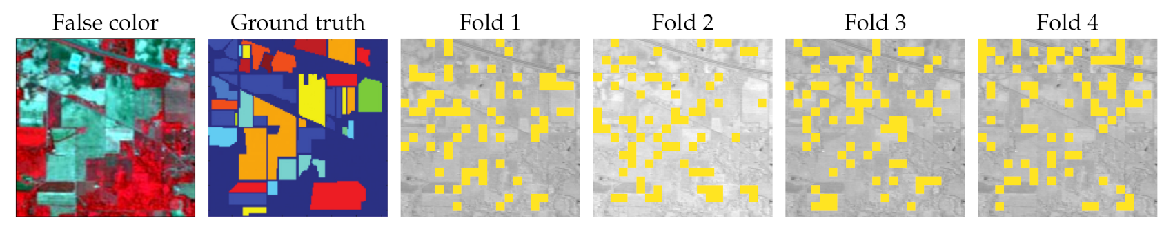
Figure 1.
The false-color version of the Indian Pines (IP) scene, alongside its ground-truth manual delineation and the folds obtained using our patch-based splitting technique [
16]. The training patches, containing all training pixels, are rendered in yellow, whereas all other areas constitute the test set.
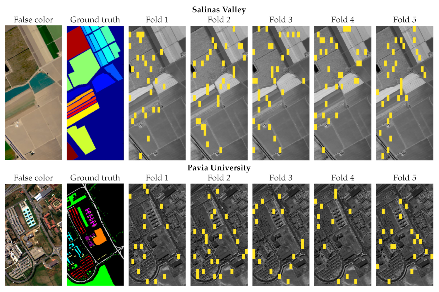
Figure 2.
The false-color versions of Salinas Valley (SV) and Pavia University (PU), alongside their ground-truth manual delineations and the folds obtained using our patch-based splitting technique [
16]. The training patches, containing all training pixels, are rendered in yellow, whereas all other areas constitute the test set.
Figure 3.
The color-composite version of Houston, alongside its ground-truth manual delineations and the folds obtained using our patch-based splitting technique [
16]. The training patches, containing all training pixels, are rendered in yellow, whereas all other areas constitute the test set.
Figure 3.
The color-composite version of Houston, alongside its ground-truth manual delineations and the folds obtained using our patch-based splitting technique [
16]. The training patches, containing all training pixels, are rendered in yellow, whereas all other areas constitute the test set.
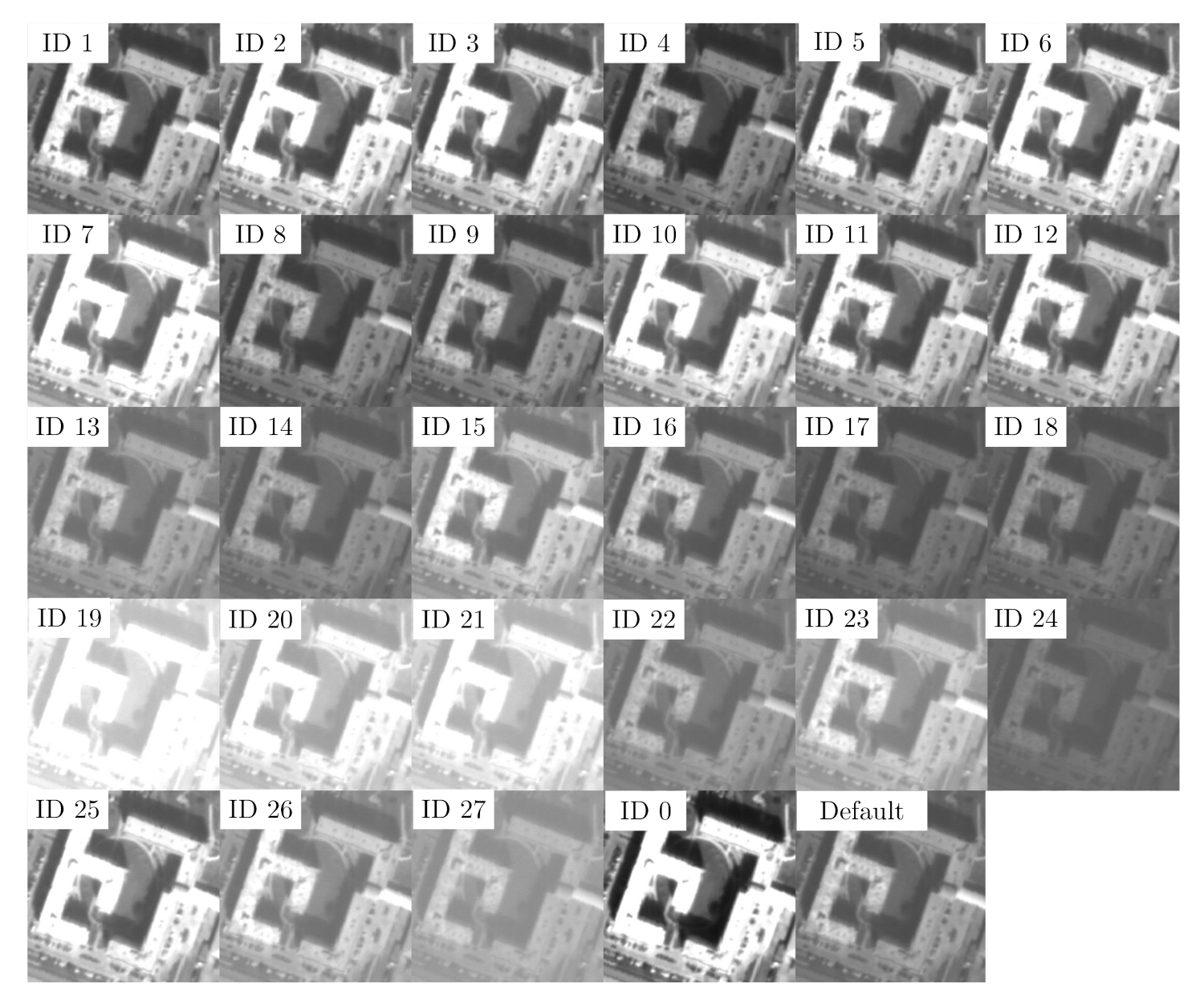
Figure 4.
An example part of the Houston scene with the investigated atmospheric disturbance variants applied (band 180)—the disturbances significantly affect the output image characteristics, hence may influence the performance of the classification algorithms.
Figure 4.
An example part of the Houston scene with the investigated atmospheric disturbance variants applied (band 180)—the disturbances significantly affect the output image characteristics, hence may influence the performance of the classification algorithms.
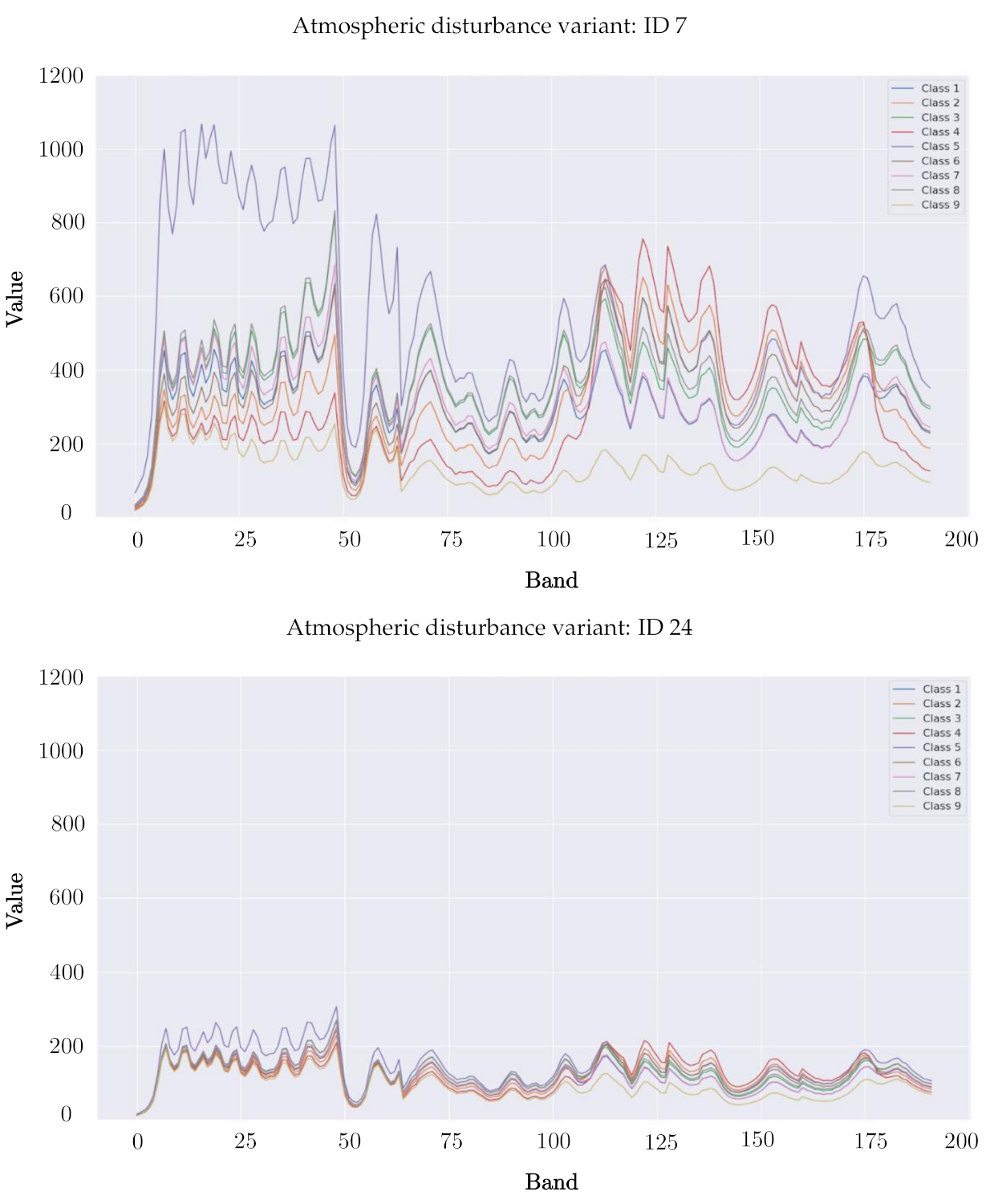
Figure 5.
The spectral profiles (averaged across all pixels, and for all classes) of the PU classes obtained for two example atmospheric disturbance variants (with IDs 7 and 24).
Figure 5.
The spectral profiles (averaged across all pixels, and for all classes) of the PU classes obtained for two example atmospheric disturbance variants (with IDs 7 and 24).
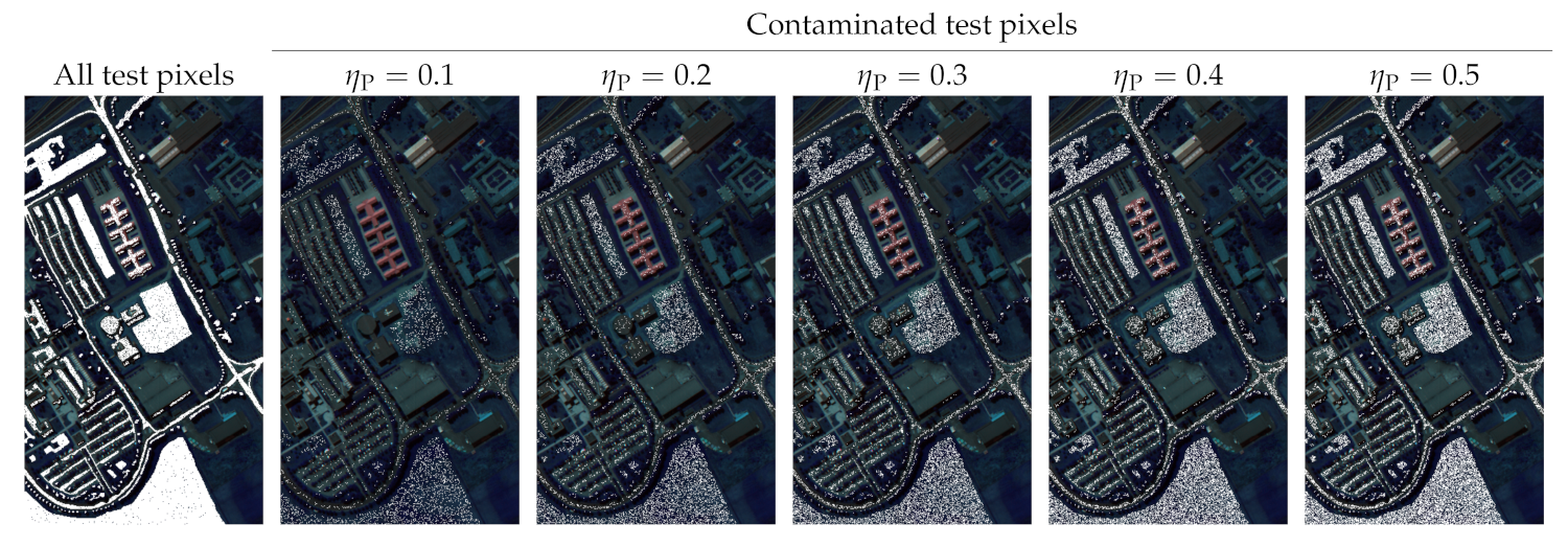
Figure 6.
All ground-truth pixels in PU (rendered in white), alongside those pixels that would be affected by our noise contamination for all investigated values (). For simplicity, we present all pixels with ground-truth labels, not just the test pixels that would result from our patch-based data splits—in the experimental study, we contaminate test sets only.
Figure 7.
The spectral profiles (averaged across all pixels) of all PU classes (for brevity, we omit the color legends in the plots—different colors present different classes) in the original data and the data contaminated with all noise distributions for and . We normalize the values to the range for readability.
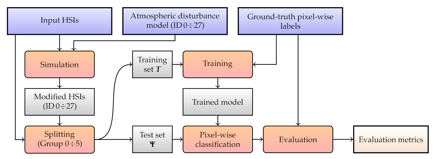
Figure 8.
A flowchart of Experiment 1. Blue rectangles indicate the input data, the red ones are the actions, and the gray ones present the artifacts, with the final outcome annotated with light gray.
Figure 8.
A flowchart of Experiment 1. Blue rectangles indicate the input data, the red ones are the actions, and the gray ones present the artifacts, with the final outcome annotated with light gray.
Figure 9.
The results obtained using 1D-CNN for all investigated groups in the Monte-Carlo cross-validation setting. We present the metrics obtained over both training and test sets, alongside the differences between the metrics elaborated for and .
Figure 9.
The results obtained using 1D-CNN for all investigated groups in the Monte-Carlo cross-validation setting. We present the metrics obtained over both training and test sets, alongside the differences between the metrics elaborated for and .
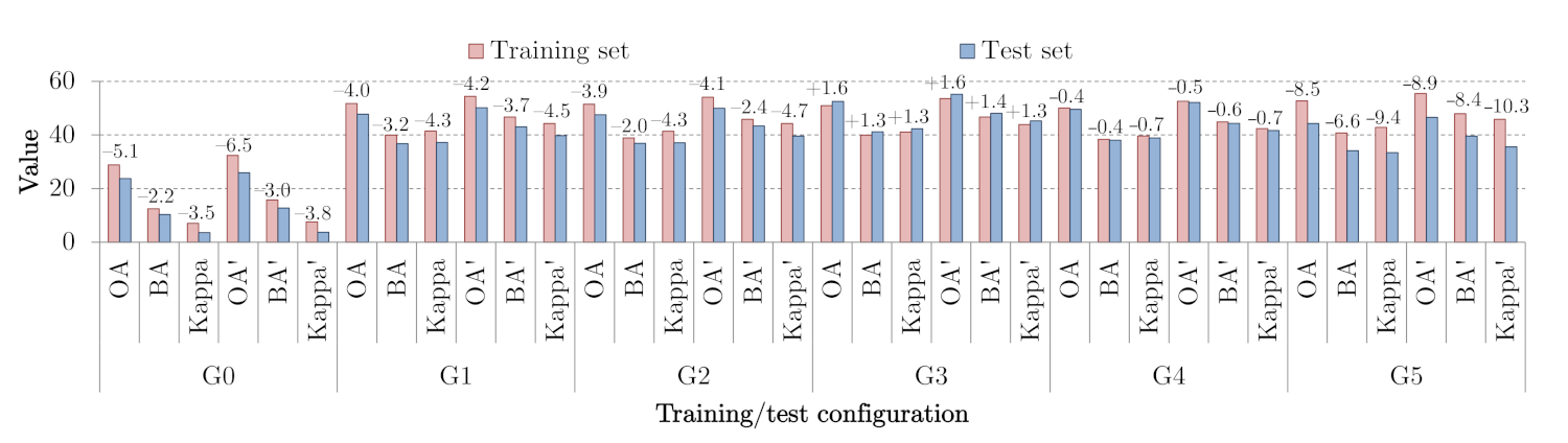
Figure 10.
The results obtained using 2.5D-CNN for all investigated groups using our patch-based training-test data splits. We present the metrics obtained over both training and test sets, alongside the differences between the metrics elaborated for and .
Figure 10.
The results obtained using 2.5D-CNN for all investigated groups using our patch-based training-test data splits. We present the metrics obtained over both training and test sets, alongside the differences between the metrics elaborated for and .
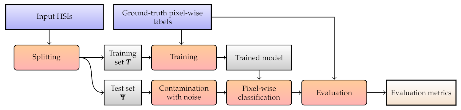
Figure 11.
A flowchart of Experiment 2. Blue rectangles indicate the input data, the red ones are the actions, and the gray ones present the artifacts, with the final outcome annotated with light gray.
Figure 11.
A flowchart of Experiment 2. Blue rectangles indicate the input data, the red ones are the actions, and the gray ones present the artifacts, with the final outcome annotated with light gray.
Table 1.
The convolutional neural network (CNN) architectures investigated in this work. For each layer, we report its hyper-parameter values, where k stands for the number of kernels (filters), s is stride, B indicates the number of hyperspectral bands, is the size of the input patch, and c is the number of classes in the dataset. The Conv, MaxPool, and FC layers are the convolutional, max-pooling, and fully-connected ones, whereas ReLU is the rectified linear unit activation function.
| Model | Layer | Parameters | Activation |
|---|
| 1D-CNN | Conv1 | k: | ReLU |
| | s: | |
| Conv2 | k: | ReLU |
| | s: | |
| Conv3 | k: | ReLU |
| | s: | |
| Conv4 | k: | ReLU |
| | s: | |
| FC1 | | ReLU |
| FC2 | | ReLU |
| FC3 | | Softmax |
| 2.5D-CNN | Conv1 | | ReLU |
| MaxPool1 | | |
| Conv2 | | ReLU |
| Conv3 | | Softmax |
| 3D-CNN | Conv1 | | ReLU |
| Conv2 | | ReLU |
| Conv3 | | ReLU |
| FC1 | | ReLU |
| FC2 | | ReLU |
| FC3 | | ReLU |
| FC4 | | Softmax |
Table 2.
The number of samples (pixels) for each class in the investigated datasets.
Table 2.
The number of samples (pixels) for each class in the investigated datasets.
| Class | Indian Pines | Salinas Valley | Pavia University | Houston |
|---|
| 1 | Alfalfa | 46 | Brocoli weeds 1 | 2009 | Asphalt | 6631 | Healthy grass | 39,196 |
| 2 | Corn-notill | 1428 | Brocoli weeds 2 | 3726 | Meadows | 18,649 | Stressed grass | 130,008 |
| 3 | Corn-mintill | 830 | Fallow | 1976 | Gravel | 2099 | Artificial turf | 2736 |
| 4 | Corn | 237 | Fallow rough plow | 1394 | Trees | 3064 | Evergreen trees | 54,332 |
| 5 | Grass-pasture | 483 | Fallow smooth | 2678 | Metal sheets | 1345 | Deciduous trees | 20,172 |
| 6 | Grass-trees | 730 | Stubble | 3959 | Bare soil | 5029 | Bare earth | 18,064 |
| 7 | Grass-pasture-mowed | 28 | Celery | 3579 | Bitumen | 1330 | Water | 1064 |
| 8 | Hay-windrowed | 478 | Grapes untrained | 11,271 | Bricks | 3682 | Red. buil. | 158,995 |
| 9 | Oats | 20 | Soil vinyard dev. | 6203 | Shadows | 947 | Non-res. build. | 894,769 |
| 10 | Soybean-notill | 972 | Corn weeds | 3278 | | | Roads | 183,283 |
| 11 | Soybean-mintill | 2455 | Lettuce 4-week | 1068 | | | Sidewalks | 136,035 |
| 12 | Soybean-clean | 593 | Lettuce 5-week | 1927 | | | Crosswalks | 6059 |
| 13 | Wheat | 205 | Lettuce 6-week | 916 | | | Major thoroughfares | 185,438 |
| 14 | Woods | 1265 | Lettuce 7-week | 1070 | | | Highways | 37,438 |
| 15 | Build.-Trees-Drives | 386 | Vinyard untrained | 7268 | | | Railways | 27,748 |
| 16 | Stone-Steel-Towers | 93 | Vinyard trellis | 1807 | | | Paved park. lots | 45,932 |
| 17 | | | | | | | Unpaved park. lots | 587 |
| 18 | | | | | | | Cars | 26,289 |
| 19 | | | | | | | Trains | 21,479 |
| 20 | | | | | | | Stadium seats | 27,296 |
| Total | | 54,129 | | 42,776 | | 10,249 | | 2,016,920 |
Table 3.
The number of pixels in each training and test set within each fold ( and , respectively) for the IP and SV scenes—we have extracted four IP and five SV folds. For each fold, we boldface the classes that are not present in , but they are captured in . Additionally, we underline those classes that are not included in , but are available in .
| | Indian Pines | Salinas Valley |
|---|
| | Fold 1 | Fold 2 | Fold 3 | Fold 4 | Fold 1 | Fold 2 | Fold 3 | Fold 4 | Fold 5 |
| Class | | | | | | | | | | | | | | | | | | |
| 1 | 0 | 46 | 0 | 46 | 18 | 28 | 18 | 28 | 222 | 1787 | 364 | 1645 | 367 | 1742 | 145 | 1864 | 63 | 1946 |
| 2 | 223 | 1205 | 433 | 995 | 412 | 1016 | 339 | 1089 | 370 | 3356 | 657 | 3069 | 126 | 3600 | 603 | 3123 | 37 | 3689 |
| 3 | 150 | 680 | 218 | 612 | 320 | 510 | 142 | 688 | 0 | 1976 | 284 | 1692 | 119 | 1857 | 82 | 1894 | 440 | 1536 |
| 4 | 37 | 200 | 29 | 208 | 73 | 164 | 98 | 139 | 0 | 1394 | 446 | 948 | 200 | 1194 | 26 | 1368 | 86 | 1308 |
| 5 | 152 | 331 | 179 | 304 | 79 | 404 | 73 | 410 | 151 | 2527 | 17 | 2661 | 96 | 2582 | 0 | 2678 | 312 | 2366 |
| 6 | 315 | 415 | 158 | 572 | 128 | 602 | 129 | 601 | 0 | 3959 | 212 | 3747 | 249 | 3710 | 454 | 3505 | 564 | 395 |
| 7 | 28 | 0 | 0 | 28 | 0 | 28 | 0 | 28 | 0 | 3579 | 316 | 3263 | 341 | 3238 | 431 | 3148 | 221 | 3358 |
| 8 | 181 | 297 | 49 | 429 | 69 | 409 | 179 | 299 | 1411 | 9860 | 890 | 10,381 | 1109 | 10,162 | 650 | 10,621 | 1039 | 10,323 |
| 9 | 2 | 18 | 14 | 6 | 4 | 16 | 0 | 20 | 220 | 5983 | 566 | 5637 | 559 | 5644 | 22 | 6181 | 433 | 5770 |
| 10 | 195 | 777 | 205 | 767 | 236 | 736 | 60 | 712 | 837 | 2441 | 439 | 2839 | 178 | 3100 | 351 | 2927 | 314 | 2964 |
| 11 | 543 | 1912 | 693 | 1762 | 561 | 1894 | 567 | 1888 | 100 | 968 | 82 | 986 | 121 | 947 | 0 | 1068 | 306 | 762 |
| 12 | 226 | 367 | 13 | 580 | 206 | 387 | 148 | 445 | 24 | 1903 | 176 | 1751 | 206 | 1721 | 174 | 1753 | 358 | 1569 |
| 13 | 72 | 133 | 56 | 149 | 39 | 166 | 38 | 167 | 41 | 875 | 107 | 809 | 156 | 760 | 76 | 840 | 14 | 902 |
| 14 | 308 | 957 | 395 | 870 | 175 | 1090 | 387 | 878 | 187 | 883 | 96 | 974 | 11 | 1059 | 143 | 927 | 5 | 1065 |
| 15 | 94 | 292 | 81 | 305 | 106 | 280 | 105 | 281 | 1310 | 5958 | 70 | 7198 | 775 | 6493 | 1615 | 5653 | 438 | 6830 |
| 16 | 0 | 93 | 0 | 93 | 76 | 17 | 17 | 76 | 29 | 1778 | 0 | 1807 | 220 | 1587 | 14 | 1793 | 220 | 1587 |
Table 4.
The number of pixels in each training and test set within each fold ( and , respectively) for the PU scene—we have extracted five folds. For each fold, we boldface the classes that are not present in , but they are captured in .
Table 4.
The number of pixels in each training and test set within each fold ( and , respectively) for the PU scene—we have extracted five folds. For each fold, we boldface the classes that are not present in , but they are captured in .
| | Fold 1 | Fold 2 | Fold 3 | Fold 4 | Fold 5 |
|---|
| Class | | | | | | | | | | |
|---|
| 1 | 437 | 6194 | 353 | 6278 | 631 | 6000 | 338 | 6293 | 897 | 5734 |
| 2 | 1577 | 17,072 | 788 | 17,861 | 1330 | 17,319 | 1942 | 16,707 | 612 | 18,037 |
| 3 | 202 | 1897 | 4 | 2095 | 132 | 1967 | 130 | 1969 | 89 | 2010 |
| 4 | 223 | 2841 | 281 | 2783 | 191 | 2873 | 112 | 2952 | 147 | 2917 |
| 5 | 0 | 1345 | 176 | 1169 | 270 | 1075 | 0 | 1345 | 191 | 1154 |
| 6 | 0 | 5029 | 392 | 4637 | 0 | 5029 | 0 | 5029 | 487 | 4542 |
| 7 | 0 | 1330 | 0 | 1330 | 0 | 1330 | 0 | 1330 | 0 | 1330 |
| 8 | 219 | 3463 | 476 | 3206 | 111 | 3571 | 98 | 3584 | 297 | 3385 |
| 9 | 87 | 860 | 121 | 826 | 70 | 877 | 0 | 947 | 94 | 853 |
Table 5.
The number of pixels in each training and test set within each fold ( and , respectively) for the Houston scene—we have extracted five folds in each version (Version A and Version B). For each fold, we boldface the classes that are not present in , but they are captured in .
Table 5.
The number of pixels in each training and test set within each fold ( and , respectively) for the Houston scene—we have extracted five folds in each version (Version A and Version B). For each fold, we boldface the classes that are not present in , but they are captured in .
| | Houston (Version A) |
|---|
| | Fold 1 | Fold 2 | Fold 3 | Fold 4 | Fold 5 |
|---|
| Class | | | | | | | | | | |
|---|
| 1 | 28 | 39,168 | 350 | 38,846 | 20 | 39,176 | 640 | 38,556 | 64 | 39,132 |
| 2 | 176 | 129,832 | 1330 | 128,678 | 2708 | 127,300 | 2184 | 127,824 | 3096 | 126,912 |
| 3 | 0 | 2736 | 424 | 2312 | 0 | 2736 | 0 | 2736 | 364 | 2372 |
| 4 | 2226 | 52,096 | 617 | 53,705 | 1351 | 52,971 | 240 | 54,082 | 303 | 54,019 |
| 5 | 0 | 20,172 | 1019 | 19,153 | 1586 | 18,586 | 288 | 19,884 | 244 | 19,928 |
| 6 | 0 | 18,064 | 1268 | 16,796 | 608 | 17,456 | 0 | 18,064 | 0 | 18,064 |
| 7 | 0 | 1064 | 0 | 1064 | 0 | 1064 | 64 | 1000 | 0 | 1064 |
| 8 | 2356 | 156,639 | 1331 | 157,664 | 2362 | 156,633 | 1487 | 157,508 | 2768 | 156,227 |
| 9 | 17,069 | 877,700 | 14,061 | 880,708 | 10,225 | 884,544 | 14,312 | 880,457 | 18,416 | 876,353 |
| 10 | 2065 | 181,218 | 3054 | 180,229 | 2298 | 180,985 | 3190 | 180,093 | 2880 | 180,403 |
| 11 | 1958 | 134,077 | 2483 | 133,552 | 2796 | 133,239 | 2179 | 133,856 | 1176 | 134,859 |
| 12 | 17 | 6042 | 0 | 6059 | 111 | 5948 | 214 | 5845 | 0 | 6059 |
| 13 | 783 | 184,655 | 1581 | 183,857 | 4130 | 181,308 | 3289 | 182,149 | 560 | 184,878 |
| 14 | 538 | 38,900 | 1076 | 38,362 | 0 | 39,438 | 0 | 39,438 | 313 | 39,125 |
| 15 | 612 | 27,136 | 456 | 27,292 | 980 | 26,768 | 64 | 27,684 | 0 | 27,748 |
| 16 | 651 | 45,281 | 285 | 45,647 | 687 | 45,245 | 1383 | 44,549 | 48 | 45,884 |
| 17 | 0 | 587 | 0 | 587 | 0 | 587 | 0 | 587 | 0 | 587 |
| 18 | 725 | 25,564 | 254 | 26,035 | 0 | 26,289 | 644 | 25,645 | 287 | 26,002 |
| 19 | 489 | 20,990 | 1154 | 20,325 | 675 | 20,804 | 253 | 21,226 | 680 | 20,799 |
| 20 | 1082 | 26,214 | 0 | 27,296 | 0 | 27,296 | 0 | 27,296 | 4 | 27,292 |
| | Houston (Version B) |
| | Fold 1 | Fold 2 | Fold 3 | Fold 4 | Fold 5 |
| Class | | | | | | | | | | |
| 1 | 3438 | 35,758 | 6504 | 32,692 | 15,154 | 24,042 | 6968 | 32,228 | 3280 | 35,916 |
| 2 | 31,392 | 98,616 | 15,376 | 114,632 | 33,968 | 96,040 | 15,498 | 114,510 | 24,282 | 105,726 |
| 3 | 1922 | 814 | 814 | 1922 | 0 | 2736 | 0 | 2736 | 0 | 2736 |
| 4 | 3705 | 50,617 | 13,902 | 40,420 | 15,346 | 38,976 | 8587 | 45,735 | 9670 | 44,652 |
| 5 | 6736 | 13,436 | 4793 | 15,379 | 2544 | 17,628 | 1985 | 18,187 | 4114 | 16,058 |
| 6 | 0 | 18,064 | 0 | 18,064 | 15,576 | 2488 | 0 | 18,064 | 2488 | 15,576 |
| 7 | 0 | 1064 | 588 | 476 | 332 | 732 | 0 | 1064 | 144 | 920 |
| 8 | 29,989 | 129,006 | 22,531 | 136,464 | 19,636 | 139,359 | 33,881 | 125,114 | 48,949 | 110,046 |
| 9 | 170,893 | 723,876 | 254,060 | 640,709 | 175,290 | 719,479 | 140,177 | 754,592 | 115,858 | 778,911 |
| 10 | 45,076 | 138,207 | 28,549 | 154,734 | 36,307 | 146,976 | 35,391 | 147,892 | 24,712 | 158,571 |
| 11 | 22,711 | 113,324 | 35,343 | 100,692 | 32,003 | 104,032 | 26,840 | 109,195 | 14,600 | 121,435 |
| 12 | 1339 | 4720 | 880 | 5179 | 1694 | 4365 | 563 | 5496 | 1469 | 4590 |
| 13 | 31,660 | 153,778 | 37,525 | 147,913 | 25,053 | 160,385 | 32,630 | 152,808 | 53,319 | 132,119 |
| 14 | 7570 | 31,868 | 0 | 39,438 | 5282 | 34,156 | 5266 | 34,172 | 16,014 | 23,424 |
| 15 | 0 | 27,748 | 4172 | 23,576 | 740 | 27,008 | 4056 | 23,692 | 10,780 | 16,968 |
| 16 | 12,783 | 33,149 | 1837 | 44,095 | 8660 | 37,272 | 11,627 | 34,305 | 11,025 | 34,907 |
| 17 | 0 | 587 | 256 | 331 | 0 | 587 | 0 | 587 | 331 | 256 |
| 18 | 8051 | 18,238 | 1126 | 25,163 | 3456 | 22,833 | 0 | 26,289 | 13,656 | 12,633 |
| 19 | 3160 | 18,319 | 1284 | 20,195 | 1345 | 20,134 | 3772 | 17,707 | 7650 | 13,829 |
| 20 | 7052 | 20,244 | 10,696 | 16,600 | 0 | 27,296 | 5242 | 22,054 | 4306 | 22,990 |
Table 6.
Standard atmospheric profiles available in the MODTRAN radiative transfer tool.
Table 6.
Standard atmospheric profiles available in the MODTRAN radiative transfer tool.
| Symbol | Model | Water Vapor (g/cm) | Ozone (atm-cm) | Surf. Air Temp. () |
|---|
| T | Tropical | 4.120 | 0.247 | 27 |
| MLS | Mid-Latitude Summer | 2.930 | 0.319 | 21 |
| MLW | Mid-Latitude Winter | 0.853 | 0.395 | |
| SAS | Sub-Arctic Summer | 2.100 | 0.480 | 14 |
| SAW | Sub-Arctic Winter | 0.419 | 0.480 | |
| US | U.S. Standard 1962 | 1.420 | 0.344 | 15 |
Table 7.
The rounded latitude and date of acquisition can be utilized to determine the atmospheric profile according to the Fast Line-of-sight Atmospheric Analysis of Spectral Hypercubes approach. The latitude of Poland, being our default coordinates, are boldfaced.
Table 7.
The rounded latitude and date of acquisition can be utilized to determine the atmospheric profile according to the Fast Line-of-sight Atmospheric Analysis of Spectral Hypercubes approach. The latitude of Poland, being our default coordinates, are boldfaced.
| Latitude | Jan–Apr | May–June | July–Oct | Nov–Dec |
|---|
| ... | ... | ... | ... | ... |
| 60 | MLW | MLW | SAS | MLW |
| 50 | MLW | SAS | SAS | SAS |
| 40 | SAS | SAS | MLS | SAS |
| ... | ... | ... | ... | ... |
Table 8.
Components of the investigated aerosol models in rural and urban sites of Central Europe.
Table 8.
Components of the investigated aerosol models in rural and urban sites of Central Europe.
| Model | Dust | Water | Soot |
|---|
| Rural-1 | 0.02 | 0.92 | 0.06 |
| Rural-2 | 0.02 | 0.82 | 0.16 |
| Rural-3 | 0.17 | 0.77 | 0.06 |
| Urban-1 | 0.02 | 0.59 | 0.39 |
| Urban-2 | 0.02 | 0.69 | 0.29 |
| Urban-3 | 0.17 | 0.61 | 0.22 |
| Continental | 0.70 | 0.29 | 0.01 |
Table 9.
The atmospheric disturbance variants reflecting the assumed acquisition scenarios (Central Europe, urban and rural areas, with Poland being our default target).
Table 9.
The atmospheric disturbance variants reflecting the assumed acquisition scenarios (Central Europe, urban and rural areas, with Poland being our default target).
| ID | Scan Date | Latitude | Atm. Profile | Aerosol Model | AOT |
|---|
| default | 2021-03-21 | 50 | MLW | Urban-3 | 0.50 |
| 0 | 2021-03-21 | 50 | — | — | — |
| 1 | 2021-03-21 | 50 | MLW | Rural-1 | 0.10 |
| 2 | 2021-07-15 | 50 | SAS | Rural-2 | 0.10 |
| 3 | 2021-03-21 | 40 | SAS | Rural-3 | 0.10 |
| 4 | 2021-03-21 | 60 | MLW | Urban-1 | 0.10 |
| 5 | 2021-07-15 | 60 | SAS | Urban-2 | 0.10 |
| 6 | 2021-07-15 | 50 | SAS | Urban-3 | 0.10 |
| 7 | 2021-07-15 | 40 | MLS | Rural-1 | 0.25 |
| 8 | 2021-10-21 | 50 | SAS | Rural-2 | 0.25 |
| 9 | 2021-10-21 | 50 | SAS | Rural-3 | 0.25 |
| 10 | 2021-07-15 | 40 | MLS | Urban-1 | 0.25 |
| 11 | 2021-07-15 | 60 | SAS | Urban-2 | 0.25 |
| 12 | 2021-03-21 | 40 | SAS | Urban-3 | 0.25 |
| 13 | 2021-10-21 | 50 | SAS | Rural-1 | 0.70 |
| 14 | 2021-10-21 | 50 | SAS | Rural-2 | 0.70 |
| 15 | 2021-03-21 | 50 | MLW | Rural-3 | 0.70 |
| 16 | 2021-03-21 | 40 | SAS | Urban-1 | 0.70 |
| 17 | 2021-10-21 | 50 | SAS | Urban-2 | 0.70 |
| 18 | 2021-03-21 | 60 | MLW | Urban-3 | 0.70 |
| 19 | 2021-07-15 | 50 | SAS | Rural-1 | 1.20 |
| 20 | 2021-07-15 | 40 | MLS | Rural-2 | 1.20 |
| 21 | 2021-07-15 | 60 | SAS | Rural-3 | 1.20 |
| 22 | 2021-07-15 | 50 | SAS | Urban-1 | 1.20 |
| 23 | 2021-07-15 | 40 | MLS | Urban-2 | 1.20 |
| 24 | 2021-10-21 | 50 | SAS | Urban-3 | 1.20 |
| 25 | 2021-07-15 | 50 | SAS | Continental | 0.25 |
| 26 | 2021-03-21 | 50 | MLW | Continental | 0.70 |
| 27 | 2021-10-21 | 50 | SAS | Continental | 1.20 |
Table 10.
The distribution of atmospheric condition variants (for details, see
Table 9) across the folds.
Table 10.
The distribution of atmospheric condition variants (for details, see
Table 9) across the folds.
| | Fold | Variants in Fold |
|---|
| (I) | Fold 1 | 1 | 8 | 9 | 13 | 16 | 23 | 26 |
| Fold 2 | 2 | 4 | 6 | 11 | 17 | 20 | 21 |
| Fold 3 | 5 | 10 | 12 | 14 | 15 | 19 | 24 |
| Fold 4 | 3 | 7 | 18 | 22 | 25 | 27 | Default |
| (II) | Fold 1’ | 1 | 3 | 8 | 9 | 16 | 23 | 26 |
| Fold 2’ | 2 | 4 | 6 | 7 | 11 | 20 | 25 |
| Fold 3’ | 5 | 10 | 12 | 14 | 15 | 19 | Default |
| Fold 4’ | 13 | 17 | 18 | 21 | 22 | 24 | 27 |
Table 11.
The average training () and inference () times (both in seconds) obtained using 1D-CNN for all investigated datasets (1D-CNN has 1.2 million trainable parameters, and 50 MFLOPs in all scenarios). The metric reflects the total inference time over all test pixels.
Table 11.
The average training () and inference () times (both in seconds) obtained using 1D-CNN for all investigated datasets (1D-CNN has 1.2 million trainable parameters, and 50 MFLOPs in all scenarios). The metric reflects the total inference time over all test pixels.
| Set→ | IP | SV | PU | Houston |
|---|
| 76.41 | 112.26 | 66.80 | 490.23 |
| 1.28 | 1.21 | 0.81 | 34.26 |
Table 12.
The average training () and inference () times (both in seconds) obtained using 2.5D-CNN for all sets, together with the numbers of trainable parameters (#P, millions), and the floating point operations (in mega FLOPs). The metric reflects the total inference time over all test pixels.
Table 12.
The average training () and inference () times (both in seconds) obtained using 2.5D-CNN for all sets, together with the numbers of trainable parameters (#P, millions), and the floating point operations (in mega FLOPs). The metric reflects the total inference time over all test pixels.
| Set | | | #P | MFLOPs |
|---|
| IP | 7225.66 | 1.61 | 0.33 | 6.23 |
| SV | 2036.66 | 3.95 | 1.56 | 45.55 |
| PU | 569.31 | 1.51 | 0.78 | 20.96 |
Table 13.
The results obtained using all investigated deep models, and averaged across all datasets (for uncontaminated test sets), folds, and executions. We boldface the best result for each metric.
Table 13.
The results obtained using all investigated deep models, and averaged across all datasets (for uncontaminated test sets), folds, and executions. We boldface the best result for each metric.
| Metric | 1D-CNN | 2.5D-CNN | 3D-CNN |
|---|
| OA | 66.37 | 58.41 | 59.95 |
| BA | 55.40 | 45.77 | 49.00 |
| 58.39 | 49.00 | 51.09 |
| OA’ | 69.18 | 62.19 | 63.75 |
| BA’ | 64.75 | 55.15 | 58.68 |
| ’ | 61.25 | 53.33 | 55.42 |
Table 14.
The average training () and inference () times (both in seconds) obtained using 1D-CNN, 2.5D-CNN, and 3D-CNN for all sets (for brevity, we refer to the A and B versions of Houston as H(A) and H(B), respectively), together with the numbers of trainable parameters of the corresponding convolutional models (#P, millions), and the floating point operations (in mega FLOPs). The metric reflects the total inference time over all test pixels.
| | 1D-CNN | 2.5D-CNN | 3D-CNN |
|---|
| Set | | | #P | MFLOPs | | | #P | MFLOPs | | | #P | MFLOPs |
|---|
| IP | 14.56 | 0.58 | 1.27 | 52.98 | 12.84 | 0.80 | 0.33 | 6.43 | 36.15 | 1.55 | 2.58 | 72.58 |
| SV | 23.84 | 1.94 | 1.27 | 53.47 | 19.28 | 6.74 | 1.64 | 48.31 | 59.32 | 7.09 | 2.63 | 74.06 |
| PU | 7.28 | 1.00 | 0.91 | 23.68 | 10.57 | 2.18 | 0.50 | 11.85 | 16.24 | 3.11 | 1.39 | 36.80 |
| H(A) | 35.99 | 8.24 | 0.67 | 8.24 | 30.62 | 70.24 | 0.34 | 6.44 | 57.67 | 80.77 | 0.74 | 17.26 |
| H(B) | 281.63 | 6.64 | 0.67 | 8.24 | 333.04 | 42.96 | 0.34 | 6.44 | 572.86 | 59.29 | 0.74 | 17.26 |
Table 15.
The differences between the values obtained for the original—uncontaminated—test sets, and the noisy ones for all classification quality metrics obtained using all deep models. The green colors indicate the smallest differences (hence the highest “robustness” against the corresponding noise distribution), whereas the orange cells highlight the largest differences.
| 1D CNN |
|---|
| | Gaussian | Impulsive | Poisson |
| 0.1 | 0.2 | 0.3 | 0.4 | 0.5 | 0.1 | 0.2 | 0.3 | 0.4 | 0.5 | 0.1 | 0.2 | 0.3 | 0.4 | 0.5 |
|
OA | 0.87 | 1.74 | 2.61 | 3.50 | 4.35 | 5.15 | 10.28 | 15.41 | 20.62 | 25.76 | 4.16 | 8.33 | 12.51 | 16.61 | 20.83 |
| BA | 0.98 | 1.92 | 2.77 | 3.76 | 4.67 | 4.91 | 9.72 | 14.68 | 19.47 | 24.36 | 3.99 | 8.04 | 12.13 | 16.07 | 20.12 |
| 1.12 | 2.23 | 3.34 | 4.48 | 5.58 | 6.03 | 11.95 | 17.87 | 23.66 | 29.46 | 4.97 | 9.94 | 14.91 | 19.76 | 24.74 |
| OA’ | −0.35 | 0.54 | 1.43 | 2.34 | 3.22 | 4.16 | 9.56 | 15.00 | 20.43 | 25.83 | 3.14 | 7.54 | 11.96 | 16.28 | 20.74 |
| BA’ | −0.60 | 0.53 | 1.54 | 2.73 | 3.81 | 4.15 | 9.97 | 15.91 | 21.71 | 27.63 | 2.96 | 7.76 | 12.62 | 17.29 | 22.10 |
| ’ | −0.71 | 0.44 | 1.59 | 2.77 | 3.92 | 4.92 | 11.51 | 18.03 | 24.52 | 30.88 | 3.51 | 8.87 | 14.22 | 19.44 | 24.79 |
| 2.5D CNN |
| | Gaussian | Impulsive | Poisson |
| 0.1 | 0.2 | 0.3 | 0.4 | 0.5 | 0.1 | 0.2 | 0.3 | 0.4 | 0.5 | 0.1 | 0.2 | 0.3 | 0.4 | 0.5 |
|
OA | 0.08 | 0.09 | 0.09 | 0.10 | 0.12 | 4.53 | 8.97 | 13.43 | 17.90 | 22.32 | 1.58 | 3.09 | 4.57 | 6.09 | 7.59 |
| BA | 0.13 | 0.15 | 0.15 | 0.16 | 0.20 | 4.05 | 7.98 | 11.87 | 15.78 | 19.68 | 1.61 | 3.08 | 4.54 | 6.01 | 7.50 |
| 0.10 | 0.12 | 0.13 | 0.14 | 0.17 | 5.03 | 9.88 | 14.69 | 19.43 | 24.15 | 2.04 | 4.01 | 5.98 | 7.99 | 10.00 |
| OA’ | 0.08 | 0.09 | 0.09 | 0.11 | 0.12 | 4.83 | 9.55 | 14.32 | 19.07 | 23.84 | 1.62 | 3.17 | 4.70 | 6.26 | 7.80 |
| BA’ | 0.16 | 0.18 | 0.18 | 0.20 | 0.23 | 4.88 | 9.61 | 14.25 | 18.94 | 23.69 | 1.93 | 3.70 | 5.46 | 7.23 | 9.02 |
| ’ | 0.10 | 0.12 | 0.13 | 0.15 | 0.17 | 5.87 | 11.57 | 17.17 | 22.68 | 28.13 | 2.11 | 4.15 | 6.18 | 8.26 | 10.35 |
| 3D CNN |
| | Gaussian | Impulsive | Poisson |
| 0.1 | 0.2 | 0.3 | 0.4 | 0.5 | 0.1 | 0.2 | 0.3 | 0.4 | 0.5 | 0.1 | 0.2 | 0.3 | 0.4 | 0.5 |
|
OA | 0.07 | 0.12 | 0.18 | 0.24 | 0.30 | 3.90 | 7.74 | 11.61 | 15.46 | 19.33 | 3.07 | 6.11 | 9.17 | 12.22 | 15.22 |
| BA | −0.04 | 0.02 | 0.09 | 0.15 | 0.21 | 4.16 | 8.43 | 12.65 | 16.92 | 21.19 | 3.21 | 6.54 | 9.85 | 13.17 | 16.45 |
| 0.03 | 0.10 | 0.17 | 0.25 | 0.32 | 5.00 | 10.01 | 15.04 | 20.07 | 25.22 | 3.82 | 7.66 | 11.55 | 15.43 | 19.29 |
| OA’ | 0.07 | 0.13 | 0.19 | 0.25 | 0.74 | 4.06 | 8.09 | 12.12 | 16.14 | 20.18 | 3.25 | 6.47 | 9.71 | 12.94 | 16.12 |
| BA’ | −0.05 | 0.03 | 0.10 | 0.16 | −0.19 | 4.96 | 10.06 | 15.06 | 20.16 | 25.26 | 3.78 | 7.70 | 11.60 | 15.50 | 19.37 |
| ’ | 0.04 | 0.11 | 0.19 | 0.27 | 0.34 | 5.51 | 11.06 | 16.61 | 22.06 | 27.67 | 4.14 | 8.28 | 12.46 | 16.62 | 20.76 |
Table 16.
The differences between the values obtained for the original—uncontaminated—test sets, and the noisy ones, obtained for the Gaussian noise with zero mean and various standard deviations () for all classification quality metrics obtained using all deep models. The green colors indicate the smallest differences (hence the highest “robustness” against the corresponding noise distribution), whereas the orange cells highlight the largest differences.
| | 1D-CNN | 2.5D-CNN | 3D-CNN |
|---|
| 0.01 | 0.05 | 0.10 | 0.25 | 0.50 | 0.01 | 0.05 | 0.10 | 0.25 | 0.50 | 0.01 | 0.05 | 0.10 | 0.25 | 0.50 |
| OA | 0.87 | 2.46 | 3.25 | 4.14 | 4.59 | 0.08 | 0.26 | 0.60 | 1.42 | 2.17 | 0.07 | 1.11 | 2.17 | 3.32 | 3.64 |
| BA | 0.98 | 2.44 | 3.20 | 4.02 | 4.54 | 0.13 | 0.38 | 0.74 | 1.59 | 2.32 | −0.04 | 1.13 | 2.35 | 3.64 | 3.99 |
| 1.12 | 3.01 | 3.93 | 4.96 | 5.51 | 0.10 | 0.36 | 0.82 | 1.87 | 2.82 | 0.03 | 1.25 | 2.58 | 4.19 | 4.73 |
| OA’ | −0.35 | 1.31 | 2.16 | 3.11 | 3.61 | 0.08 | 0.29 | 0.61 | 1.47 | 2.27 | 0.07 | 1.17 | 2.32 | 3.56 | 3.91 |
| BA’ | −0.60 | 1.12 | 2.02 | 3.00 | 3.62 | 0.16 | 0.45 | 0.88 | 1.87 | 2.76 | −0.05 | 1.26 | 2.71 | 4.31 | 4.75 |
| ’ | −0.71 | 1.31 | 2.33 | 3.49 | 4.12 | 0.10 | 0.38 | 0.84 | 1.94 | 3.00 | 0.04 | 1.35 | 2.82 | 4.62 | 5.23 |


 ,
, 


