Examining the Links between Multi-Frequency Multibeam Backscatter Data and Sediment Grain Size

Abstract

Acoustic methods are routinely used to provide broad scale information on the geographical distribution of benthic marine habitats and sedimentary environments. Although single-frequency multibeam echosounder surveys have dominated seabed characterisation for decades, multifrequency approaches are now gaining favour in order to capture different frequency responses from the same seabed type. The aim of this study is to develop a robust modelling framework for testing the potential application and value of multifrequency (30, 95, and 300 kHz) multibeam backscatter responses to characterize sediments’ grain size in an area with strong geomorphological gradients and benthic ecological variability. We fit a generalized linear model on a multibeam backscatter and its derivatives to examine the explanatory power of single-frequency and multifrequency models with respect to the mean sediment grain size obtained from the grab samples. A strong and statistically significant (p < 0.05) correlation between the mean backscatter and the absolute values of the mean sediment grain size for the data was noted. The root mean squared error (RMSE) values identified the 30 kHz model as the best performing model responsible for explaining the most variation (84.3%) of the mean grain size at a statistically significant output (p < 0.05) with an adjusted r² = 0.82. Overall, the single low-frequency sources showed a marginal gain on the multifrequency model, with the 30 kHz model driving the significance of this multifrequency model, and the inclusion of the higher frequencies diminished the level of agreement. We recommend further detailed and sufficient ground-truth data to better predict sediment properties and to discriminate benthic habitats to enhance the reliability of multifrequency backscatter data for the monitoring and management of marine protected areas.

1. Introduction

Multibeam echosounders (MBES) have become the instrument of choice for observing and mapping the marine environment [1,2,3,4,5]. While they are routinely used in hydrography, navigational charting, offshore resource exploration, and geology, their application to ecological baseline and monitoring surveys is still developing [1,6]. Data acquired using MBES surveying provide broad-scale information about the geographical range and distribution of marine habitats on the seafloor. For ecological applications, the benefits of these MBES datasets have still not been fully optimized because of a lack of scale consideration between available lower resolution (~5 m scale) remote sensing data and the actual representation of relevant features in the marine environment (<1 m resolution) on MBES [5]. Several attempts have been made to statistically quantify the benefits of multivariate approaches to enhance seafloor characterization [1,7,8,9,10], but none of these yields sufficient evidence to evaluate the discriminatory power of multifrequency backscatter specifically with respect to sediment grain size.

Generally, marine surveys are expensive to conduct, so there is great benefit in maximizing the information derived from them [11]. New ideas in seafloor mapping continue to emerge in terms of MBES data acquisition (e.g., multifrequency) and processing (e.g., object-based image analysis and automatic feature identification). These emerging developments have the common goal of maximizing the value of MBES data (backscatter and bathymetry) to support marine spatial planning more effectively, as well as the design, monitoring, and management of marine protected areas [2,7,12,13]. Traditionally, backscatter data and its derivates relied on single-frequency MBES systems, which acquire data across narrow bandwidths [4,5,14]. With the upgrade in sonar technology and the growing scientific interest in wider bandwidth data, multifrequency backscatter acquisition is now routinely achievable [1,3,7,9,15,16,17]. This area of marine research is motivated by advances in the multispectral satellite remote sensing of terrestrial environments, which provides clear wavelength separation of multiple land cover types and terrestrial features. Spectral reflectance responses of different features on land (e.g., bare soil and different vegetation types) have been demonstrated to provide improved discrimination for detailed terrestrial mapping [18,19,20]. However, in aquatic environments, multispectral remote sensing is restricted to shallow coastal areas because of the heavy attenuation of electromagnetic radiation (EMR) in the water column [21], making acoustic MBES systems the preferred choice for seafloor mapping.

Multibeam survey strategies are generally optimized for the acquisition of bathymetry (travel-time) data, often ignoring the ecological and geological value of backscatter (amplitude) data [5], although there are significant efforts underway to highlight the importance of these data and to standardize their acquisition and processing [6]. Measured backscatter is a function of surface and volume scattering, which are in turn functions of operating frequency, grazing angle, and sediment characteristics. The frequency-dependence element of the backscatter strength is strongly linked to (i) the dominant scattering regime (interface or volume scattering), (ii) seabed roughness (across scales from sediment grain size to local slope), and (iii) the responses by volume scattering related to signal penetration [6]. In terms of the physics of scattering, surface scattering is directly proportional to seabed roughness (sediment grain size and bedforms) relative to the sonar frequency, while volume scattering is dominantly controlled by the distribution of scatterers (such as shells) below the seabed and acoustic attenuation, which again is frequency-dependent. Gaida et al. [9], supports the idea that fine sediments are better discriminated using low frequency acoustic signals linked to high signal penetration. Site specific studies have demonstrated that fine sediments have variable frequency responses [17]. Until now, no single study has yielded sufficient evidence to address the limitations and challenges of working with multifrequency backscatter data. A number of concerns have been raised in relation to the interpretation of backscatter data, including the lack of absolute sonar beam calibration, which makes it hard to accurately quantify seafloor properties [22], the lack of repeatability and comparability as a result of varying survey approaches [16], and the issue that backscatter measurements are not fully supervised and standardized [6]. Again, the physical relationships between multiple frequencies and different sediment types are complicated, and the various contributions cannot be separated [23].

Statistical relationships between backscatter data and surficial sediment properties have been proposed [14,24,25], but mostly based on single-frequency data. These approaches (including univariate and multivariate techniques) require that the backscatter data be segmented prior to the analysis or production of benthic habitat maps [5,26]. Given the aforesaid, the two dominant techniques reported for extracting statistical variables from the backscatter data include first order statistics (mean and standard deviation) and second order statistics, with the latter derived from spectral and textural analyses [2,7,16,23,27]. These approaches are also preferred as they make it possible to extract multiple features from the data that can serve as inputs for other techniques, such as automated object-based classification [9,28]. Automating the segmentation of backscatter data can also provide more reliable, repeatable, and objective outputs compared with traditional expert (“by eye”) interpretation methods (e.g., [10]). With the increasing availability of multifrequency backscatter data, our capacity to test the acoustic responses of marine sediments is greatly enhanced. A better understanding of surficial sediments is essential for many seafloor mapping applications, including habitat mapping, installation of underwater infrastructure, and mining, among other uses [5,7]. However, key questions remain regarding whether using multifrequency backscatter data combined with its derivatives will improve our ability to reliably determine sediment grain size [7,9,29,30].

To address these questions, we apply a generalized linear model (GLM) on a multifrequency MBES backscatter dataset (30, 95, and 300 kHz) collected over Hempton’s Turbot Bank (HTB) off the north coast of Ireland. These data were collected by a multi-institutional team of scientists working under the umbrella of the Marine Protected Area Monitoring and Management (MarPAMM) cross-border project [31]. This project is one of three that are active in the region, the other sister projects being the Collaborative Oceanography and Monitoring for Protected Areas and Species (COMPASS) and SeaMonitor, which is focused on marine species tracking and telemetry. Our study is concerned with providing a robust modelling framework for analysing archival and new datasets to critically examine the explanatory power of multifrequency backscatter and single-frequency data, and to determine the sediment grain size covering areas with strong geomorphological gradients and associated seabed ecological variability. The seafloor in the study area, a special area of conservation (SAC) designated under the EU Habitats Directive (92/43/EEC), comprises sand and gravel mixtures [32,33]. Our objectives were to (i) examine the multifrequency backscatter responses for discriminating different substrate types, (ii) develop a suitable semi-automated workflow for deriving and selecting secondary derivatives (texture features) from multifrequency backscatter data, (iii) examine the statistical relationship between multifrequency backscatter data and texture with sediment grain size, and (iv) use the derived variables to model and predict sediment grain size. An improved understanding of the multifrequency responses of sediments will allow for enhanced reliability of the multifrequency backscatter, and for better discrimination and subsequent mapping of benthic habitats with minimal information loss.

2. Materials and Methods

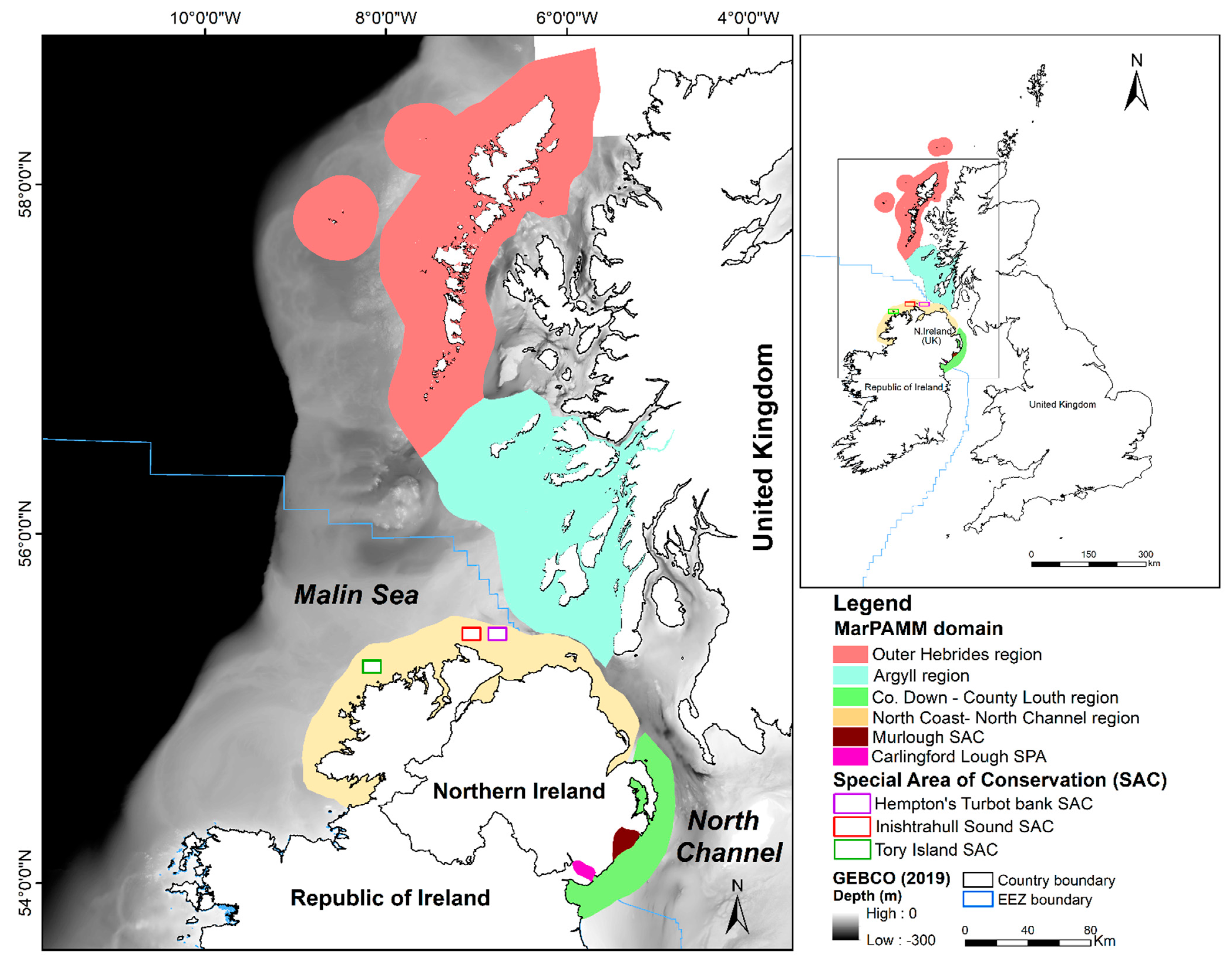
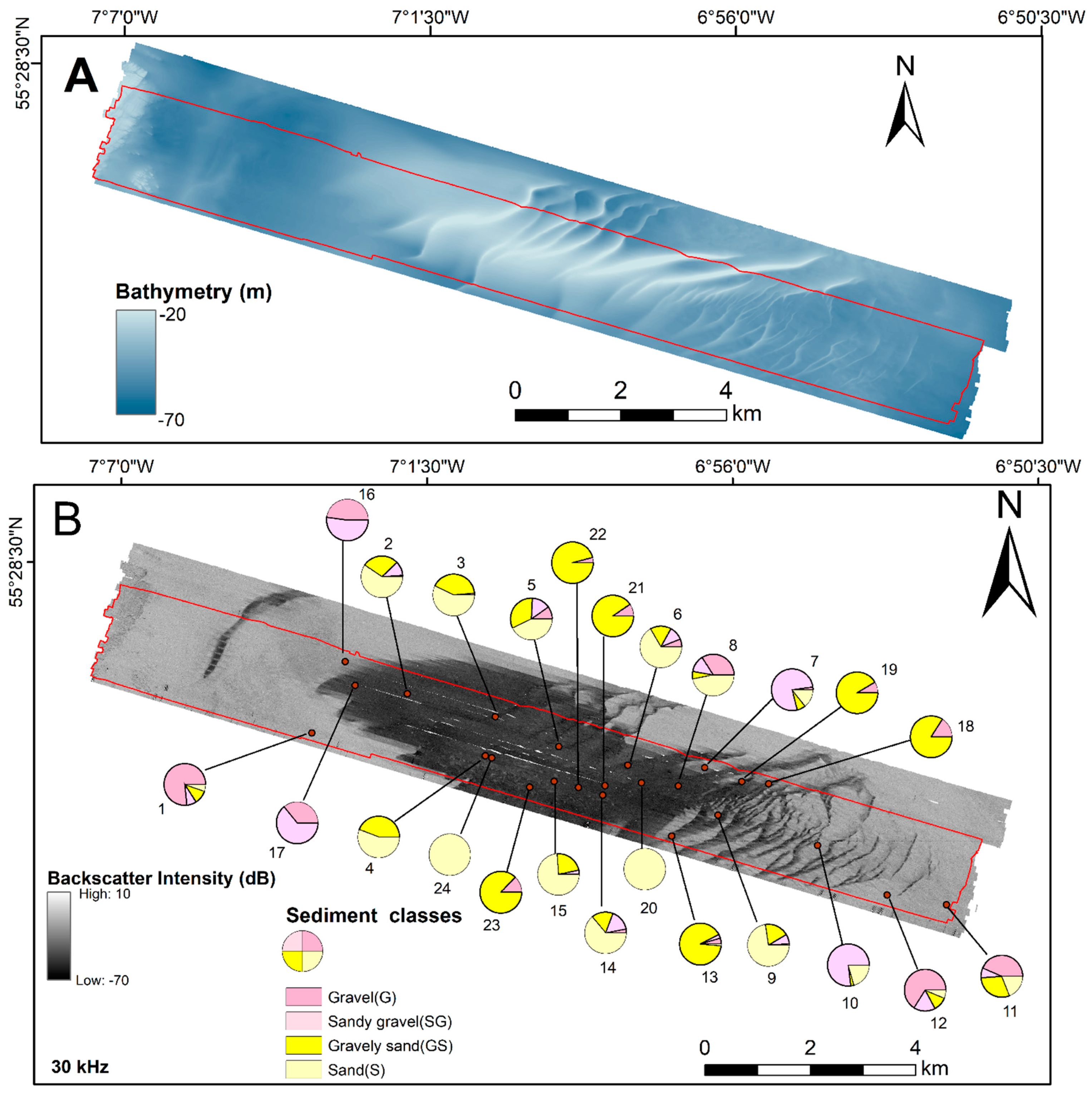
2.1. Description of Study Area

The study was carried out on Hempton’s Turbot Bank (HTB) off the north coast of Ireland. This special area of conservation (site code 002999) is designated as a sand bank priority geological feature (no. 1110 on Annex II of the E.U. Habitats Directive). The bank is part of a larger complex geological formation that extends on both sides of the Irish–U.K. border [33,34]. This SAC plays a significant ecological role by being home to burrowing lesser (Ammodytes marinus) and greater sand eels (Hyperoplus lanceolatus), which are both critical forage species that serve as an important prey for predatory seabirds, piscivorous commercial fish, and marine mammals. The HTB SAC is also a component of an inter-connected network of marine protected areas that support fish larval dispersal and migration among other ecosystem functions [35].

Our study area is located at approximately 55.4407°N, 6.9708615°W, with water depths ranging from 20 m to 70 m (Figure 1). The sand feature under investigation covers a narrow stretch (approximately 17 km in length and 2 km in width), which is within the north coast/north channel region of the MarPAMM project domain (Figure 1). The sand bank was previously surveyed under the Joint Irish Bathymetry Survey (JIBS) and the Mapping of European Seabed Habitats (MESH-Interreg IIIb) project because of its ecological significance and proximity to Inishtrahull Sound, an area of interest for marine renewable energy because of the strong currents and tidal streams.

The seafloor in the study area is heterogeneous, comprising of gravel, cobbles, boulders, sand, and mixed sand with shells. The study site includes large asymmetric sand waves [33,36], which are characterized by a low-backscatter response relative to the surrounding coarser sediment (Figure 2). These sand waves are mobile [33] and cover a tidal sandbank feature [37]. In addition, the presence of the Islay front, which is a key oceanographic feature of the Irish continental shelf [38], the strong hydrodynamic conditions in terms of current velocity and bed stress, and strong geomorphological gradients, form a strong basis for interrogating the multifrequency backscatter responses of sediments [33].

2.2. Acoustic Data Acquisition and Processing

We used two coincident MBES survey datasets from the Hempton’s Turbot Bank SAC—one collected in 2013 and the other repeated in 2019. The 2013 RV Celtic Voyager survey used a dual-head Kongsberg Simrad EM3002 (300 kHz) system, and the 2019 RV Celtic Explorer survey used Kongsberg Simrad EM302 (30 kHz) and EM1002 (95 kHz) systems. The acoustic wavelength therefore ranged from 50 to 5 mm. Positioning was provided by a Kongsberg SDP-10 (DP1), and variations in the heave, roll, and pitch were corrected for using a Kongsberg Simrad Seapath 200 motion reference system. Multibeam data were acquired using the Kongsberg Seafloor Information System (SIS) v.5.2. Sound velocity profiles (SVPs) were derived from CTD (conductivity, temperature, and depth) casts.

The bathymetry data were cleaned and tidally corrected in CARIS HIPS and SIPS v.9.1 and were exported at a 2 m spatial resolution. Three single-frequency backscatter mosaics were processed and generated using QPS Fledermaus Machine Geocoder Toolbox (FMGT v.7.8.9) software. These backscatter mosaics were corrected and normalized for angular varying gains (AVG), using an average angular response curve at a 300-window size and an adaptive AVG normalization band [6]. Processed backscatter outputs at a 0.5 m spatial resolution were exported as ASCII grids. A fourth multifrequency backscatter mosaic was generated using principal component analysis (PCA) in R software’s (v.3.6.0) RStoolbox (v.0.2.6) package from these three single-frequency mosaics, whose ship tracks had a similar survey direction with a 100% spatial overlap. Here, the first principal component that explained the highest variance (82%) was retained and exported as a raster object for further analysis. The PCA is an ordination technique used to denoise and reduce high dimensionality between datasets, while retaining the most useful data and patterns [39]. This was the preferred method for including multiple source data while capturing the fine scale variance introduced by the frequency response but avoiding artificially inflating the model performance because of collinearity.

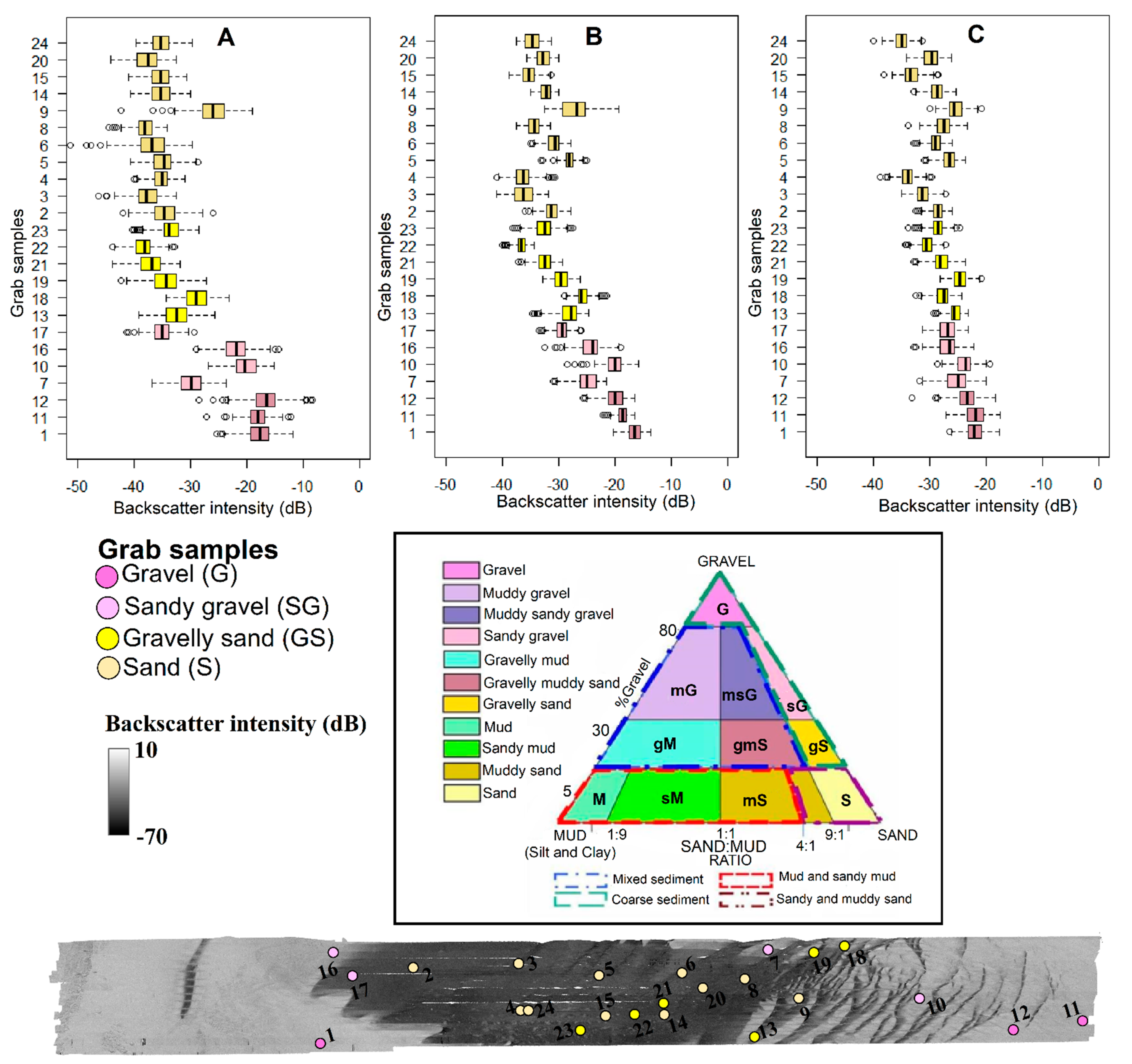
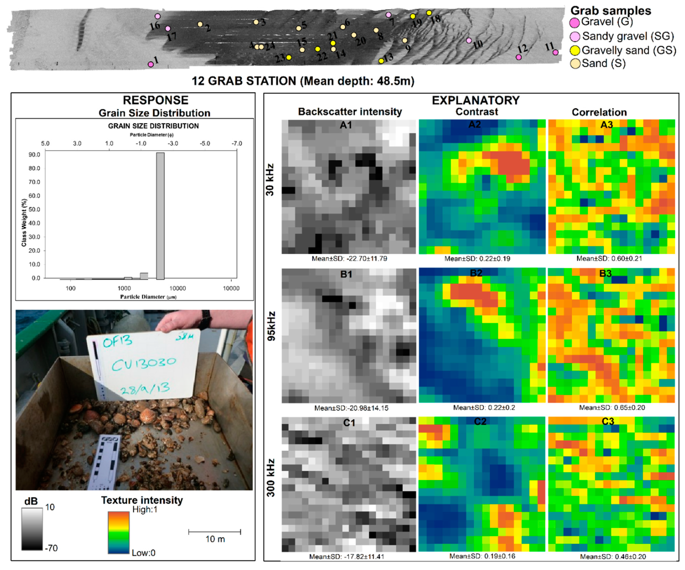
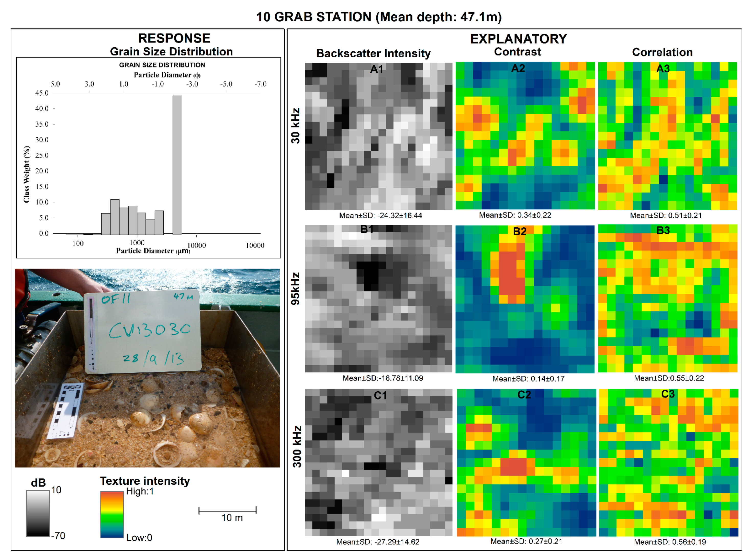
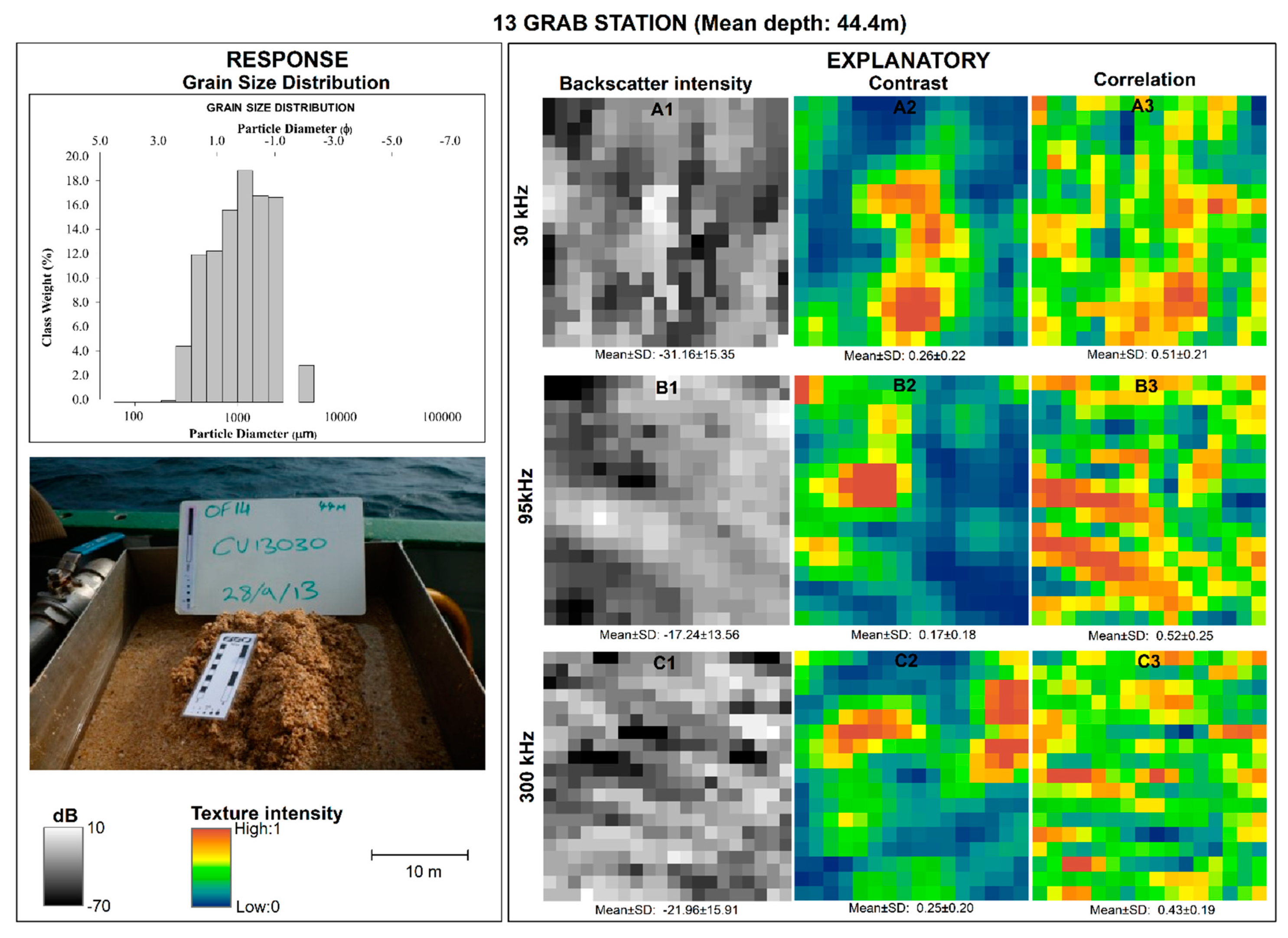
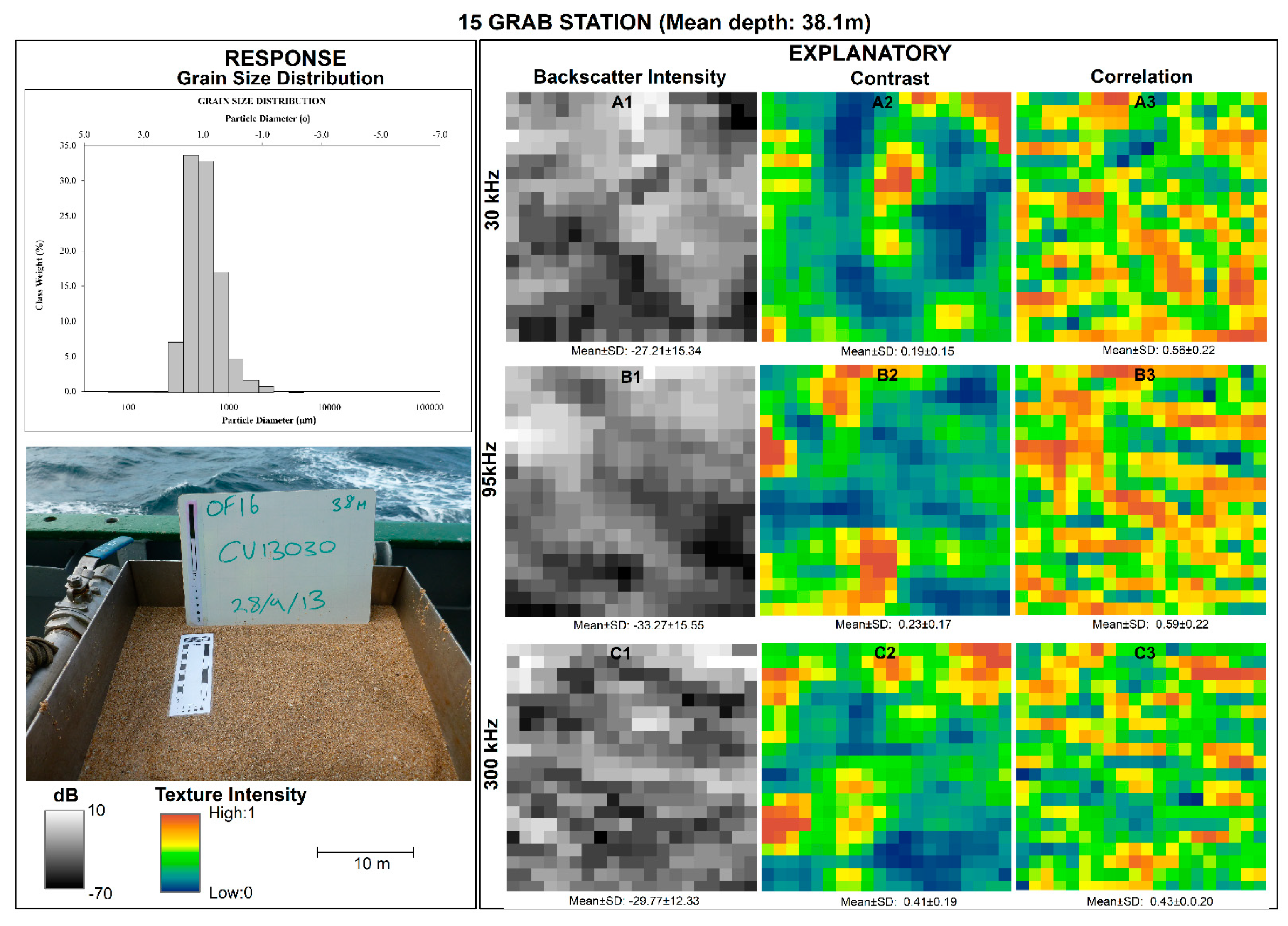
2.3. Sediment Sampling and Grain Size Analysis

Twenty-four sediment samples collected using a day grab were available for this study. Fifteen samples were collected by Ulster University in 2013 (CV13030) and nine samples were collected during a 2004 INFOMAR cruise (CE0402; Figure 2). The sampling locations were determined based on the interpretation of backscatter data, where variability in acoustic facies was qualified [33,36]. To account for the temporal offset between the collection of sediment samples and acoustic data, we analyzed the multibeam data for geomorphological changes between surveys. Difference-modelling of the 2013–2019 MBES bathymetry datasets and a comparison of the backscatter mosaics confirmed little movement in bedforms or facies’ boundaries between successive surveys. This analysis mitigates the potential effect of temporal change over the period between the surveys, especially for dominant coarser materials that better reflect the hydrodynamic conditions of the area [33,35]. We acknowledge that the temporal effect on the finer sediments cannot be fully discounted. Grab samplers were deployed across gradational areas between substrate types, taking into consideration the effect of wind, tides, and positional accuracy. A photograph of the sediment samples for each of the sampling stations together with an identification tag was taken immediately after recovery on deck. The samples were weighed, washed, and wet-sieved at 63 microns to determine the proportion of mud that was negligible. The remaining sediment samples were oven-dried, weighed, and sieved at varying mesh sizes [33]. The grain size distribution and statistics (mean and median) were computed using Gradistat v.4.0 [33]. We applied the Folk sediment classification scheme [32] on the 24 grab samples, from which we distinguished four main substrate classes, namely: gravel (G), sandy gravel (SG), gravelly sand (GS), and sand (S).

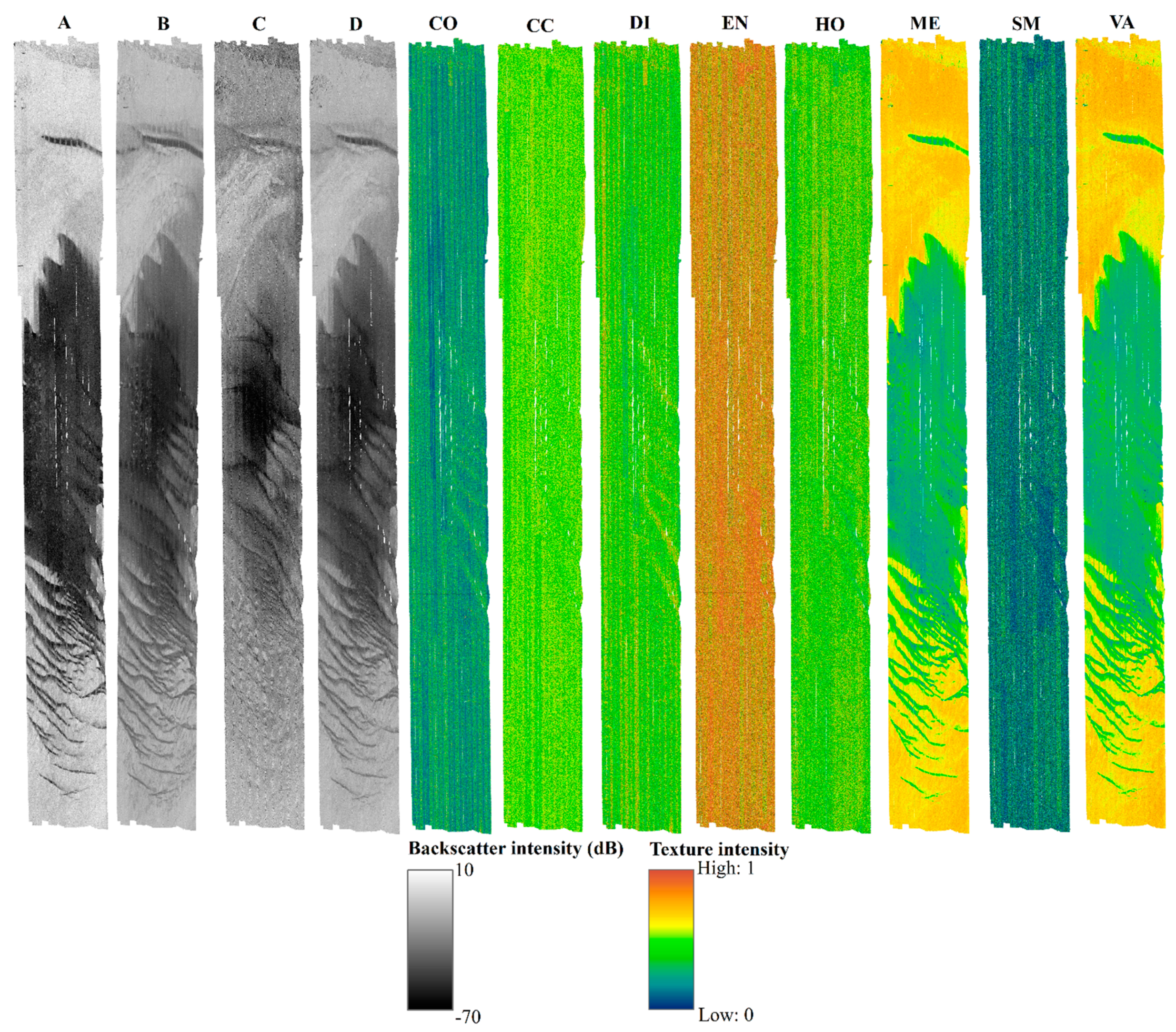
2.4. Texture Extraction

Texture denotes the spatial distribution of intensity levels in a pixel neighbourhood of an image. Different approaches have been developed for texture analysis for various applications. In the marine science domain, the grey level co-occurrence matrix (GLCM) method is widely utilized [2,7,23,27,30,40]. Basically, GLCM provides information about the number of pixel combinations that are separated by a specified distance in each direction [30]. A detailed description of the principles and theory of GLCM is given by the authors of [41] and [42]. Haralick texture features based on GLCM were derived in R software (v.3.6.0) using the GLCM package (v.1.6.5), and a visual comparison of these features is given in Figure 3. Eight texture features were generated for each of the four backscatter mosaics described earlier (three single-frequency backscatter mosaics (30, 95, 300-kHz) and one multifrequency backscatter mosaic derived from the PCA analysis) in a high-performance computing (HPC) environment (

Table A1. A list and description of Haralick texture features (Source: Lu & Batistella, 2005).

Features	Description	Equation
Contrast	Measures local variations in the GLCM.	$\mathrm{Co}={\displaystyle \sum }_{\mathrm{i},\mathrm{j}=0}^{\mathrm{N}-1}\mathrm{i} P_{\mathrm{i}, \mathrm{j}{\left(\mathrm{i}-\mathrm{j}\right)}^2}$
Correlation	Measures the joint probability occurrence of the specified pixel pairs.	$\mathrm{CC}={\displaystyle \sum }_{\mathrm{i},\mathrm{j}=0}^{\mathrm{N}-1}\mathrm{i} P_{\mathrm{i},\mathrm{j}}\left[\frac{\left(\mathrm{i}-ME\right)\left(\mathrm{j}-ME\right)}{\sqrt{{\mathrm{VA}}_{\mathrm{i}}}{\mathrm{VA}}_{\mathrm{j}}}\right]$
Dissimilarity	Measures mean of the grey level distribution of the image.	$\mathrm{DI}={\displaystyle \sum }_{\mathrm{i},\mathrm{j}=0}^{\mathrm{N}-1}\mathrm{i} P_{\mathrm{i},\mathrm{j}}\left|\mathrm{i}-\mathrm{j}\right|$
Entropy	Measures the lack of spatial organization in computational window.	$\mathrm{EN}={\displaystyle \sum }_{\mathrm{i},\mathrm{j}=0}^{\mathrm{N}-1}\mathrm{i} P_{\mathrm{i},\mathrm{j}}\left(-\ln P\mathrm{i},\mathrm{j}\right)$
Homogeneity	Measures closeness of the distribution of elements in the GLCM to the GLCM diagonal.	$\mathrm{HO}={\displaystyle \sum }_{\mathrm{i},\mathrm{j}=0}^{\mathrm{N}-1}\mathrm{i} \frac{P_{\mathrm{i},\mathrm{j}}}{1+\left(\mathrm{i}-\mathrm{j}\right)}$
Mean	Measures the average of the grey levels.	$\mathrm{ME}={\displaystyle \sum }_{\mathrm{i},\mathrm{j}=0}^{\mathrm{N}-1}\mathrm{i} P_{\mathrm{i},\mathrm{j}}$
Second moment	Measure of heterogeneity that has higher weights on differing intensity level pairs that deviate more from the mean.	$\mathrm{SM}={\displaystyle \sum }_{\mathrm{i},\mathrm{j}=0}^{\mathrm{N}-1}\mathrm{i} P_{\mathrm{i},\mathrm{j}}2$
Variance	A measure of uniformity that gives the sum of squared elements in the GLCM (also known as uniformity).	$\mathrm{VA}={\displaystyle \sum }_{\mathrm{i},\mathrm{j}=0}^{\mathrm{N}-1}\mathrm{i} P_{\mathrm{i}},\mathrm{j}{\left(\mathrm{i}-ME\right)}^2$

). These GLCM features were analyzed based on the smallest 3 x 3 pixel moving window in each of the four angular directions (0°, 45°, 90°, and 135°). The averages of these angular GLCM features were computed to obtain rotationally invariant features and were later exported as 256 bit or grey level images [30]. At each of the twenty-four sediment samples located within the common analysis area, a 10x10 m analysis window centered on the grab sample location was extracted for each GLCM derivative, resulting in 768 features for analysis (4 mosaics * 8 texture features * 24 sub-images).

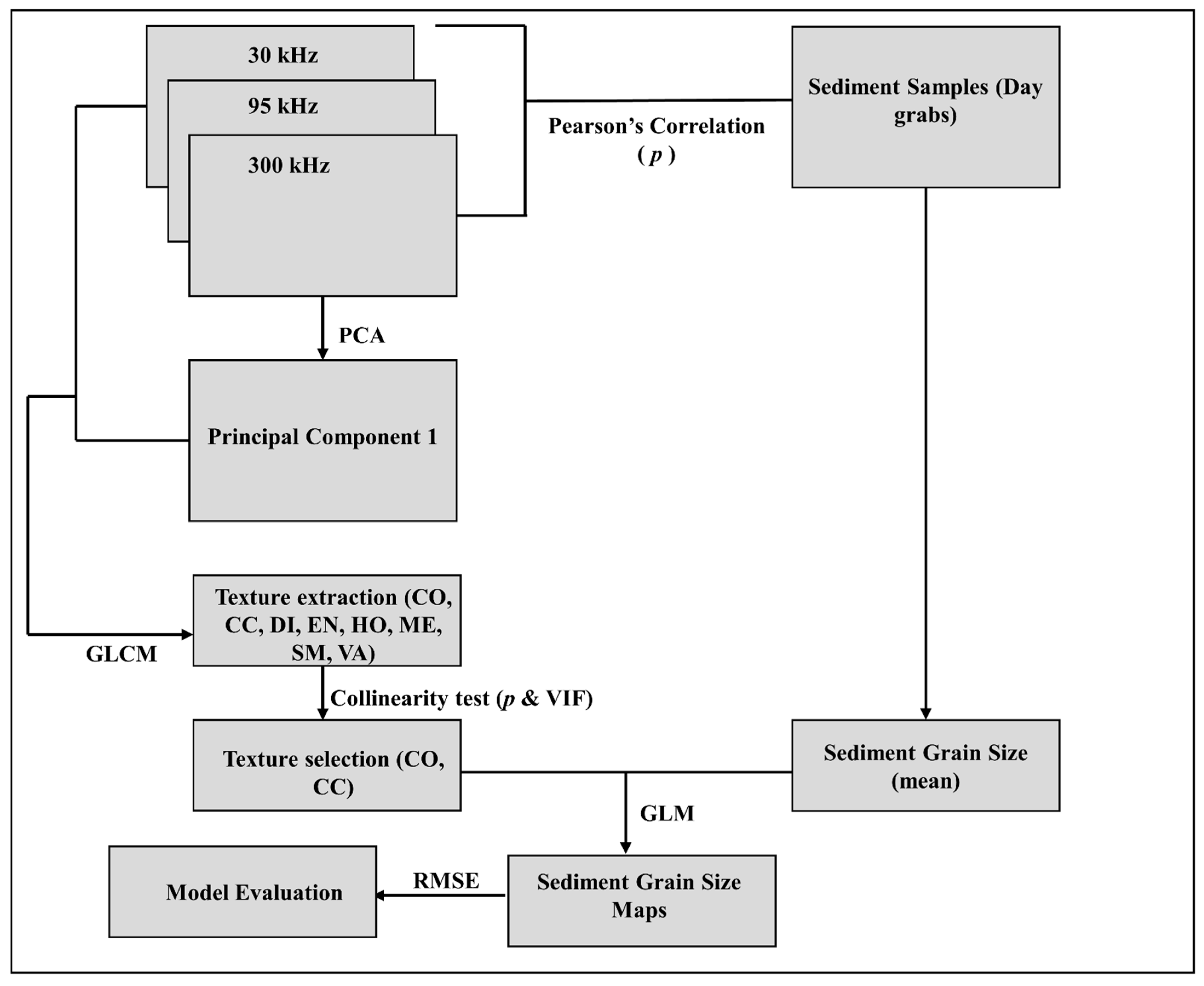
2.5. Statistical Analysis and Modelling

The analysis involved a combination of graphical and image interpretation, as well as statistical modelling of the multifrequency backscatter imagery, texture features, and sediment grain size data (Figure 4). Exploratory analyses on both mean and median (d50) sediment grain size showed that d50 did not change the statistical inference. In this study, we used mean grain size as the response variable, and mean multifrequency backscatter and their GLCM features were the explanatory variables computed on a 10 × 10 m analysis window [15]. We initially compared the multifrequency backscatter responses of the four sediment classes (G, sG, gS, and S) using conditional boxplots showing the spread of the backscatter intensity values produced in the R software (v.3.6.0) under the ggplot2 (v.3.3.0) package. This was followed by a visual comparison between backscatter, GLCM texture with sediments that involved images of explanatory variables extracted from 10x10 m rasters at four stations representative of each sediment group: 12 (gravel), 10 (sandy gravel), 13 (gravelly sand), and 15 (sand).

Based on an exploration analysis of the data and on the recommendations by [43], we carried out a two-step multicollinearity test between all eight GLCM features (Figure 3) per frequency. Before applying the GLM on the data, we first performed a pairwise pixel-by-pixel correlation using Pearson’s correlation coefficient between the 10 × 10 m image GLCM features (e.g., contrast vs. homogeneity). Where a Pearson’s correlation coefficient of p ≥ 0.7 was observed, the variables were considered collinear and one of the variables was removed from the subsequent analysis. As the mean values from each 10 × 10 m analysis window were used as the predictor variables in a GLM framework, a second multicollinearity test was passed on these variables. Predictor variables that had a variance inflation factor (VIF) >5 were eliminated from the final GLM model. Severe multicollinearity between predictor variables was known to amplify the estimation error of the model coefficients [44,45].

We fitted a generalized linear model (GLM) on the mean values of the retained predictors (backscatter features and GLCM) to test and compare the explanatory power of single-frequency vs. multifrequency backscatter with respect to the mean sediment grain size at a p < 0.05 significance level [14,25,46,47]. The response variable (mean sediment grain size) was modelled using a Gaussian distribution with an identity link function. We later progresses to generate four GLM models from the four primary mean backscatter features (30, 95, and 300 kHz and multifrequency backscatter) and the retained calculated contrast and correlation GLCM variables [7,48]. The GLM model used in this paper assumed independence of observations in the response variables and homogeneity of variance. The generalized linear model (GLM) was made up of a linear predictor [49]:

$$\eta i=\beta 0+\beta 1x1i+\dots +\beta pxpi{,}_{ }$$

(1)

where $\eta i$ is the mean response,$\beta$ is the estimators, and $x$ are the independent variables. There are two functions, as follows:

• a link function that describes how the mean,

$$E\left(Yi\right)=\mu i,$$

(2)

depends on the linear predictor

$$g\left(\mu i\right)=\eta i$$

(3)

• a variance function that describes how the variance (var (Y_i)) depends on the mean

var (Y_i) = φV (µ)

(4)

where the dispersion parameter $\phi$ is a constant.

The model evaluation was achieved using a leave one out cross-validation (LOOCV) procedure on all 24 samples in R software (v.3.6.0) using the Caret (v.6.0-86) package, which is a K-fold cross validation with a K equal to N (the number of data points in the dataset). LOOCV provides a robust estimate of the model performance that is unbiased [31]. We used root mean squared error (RMSE) metrics calculated from LOOCV to compare the performances of the four models, respectively. The RMSE values were specifically designed for model validation and selection, especially where problems of overfitting and underfitting were expected in a multivariate regression modelling framework [50]. Therefore, lower RMSE values favoured models that better fit the data, and achieved the highest prediction of the response variable [51]. In addition, residual plots of fitted verses residuals for each of the models are given in the appendix (Appendix A, Figure A1).

3. Results

3.1. Acoustic Discrimination of Sediments

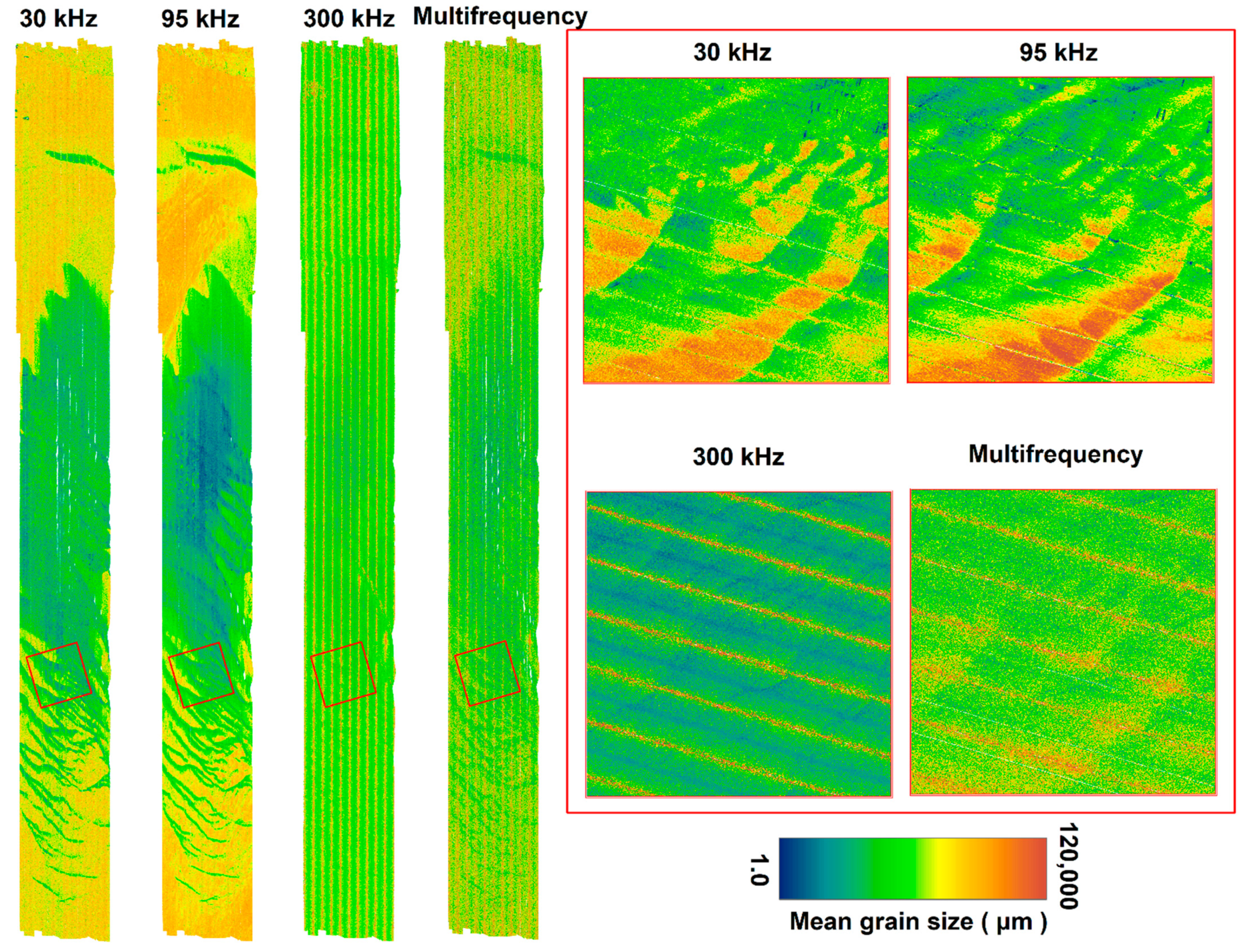
3.1.1. Multifrequency-Based Acoustic Discrimination

The four sediment types identified under the Folk classification scheme formed the units of comparison between the sediment types and backscatter signatures at multiple frequencies. The wide overlap between the maximum (−10 dB) and minimum (−50 dB) relative backscatter intensity was clear for 30 kHz, 95 kHz, and 300 kHz (Figure 5). Gravelly sediments had a higher backscatter response, while sandy sediments were characterized by relatively lower backscatter signals. Meanwhile, sand showed a wider spread in backscatter responses than the other sediment groups, which was the highest for 30 kHz ranging between −15 dB and −45 dB (Figure 5A), and lowest for 300 kHz (Figure 5C). These differences in acoustic responses made it easy to discern gravel from sand, especially for the 30 kHz data, which showed the widest separation in the backscatter responses of sediments. The 300 kHz data appeared to have a relatively low discriminatory power, as the backscatter responses for all sediments were near-identical.

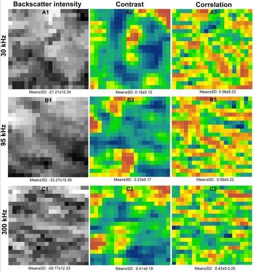
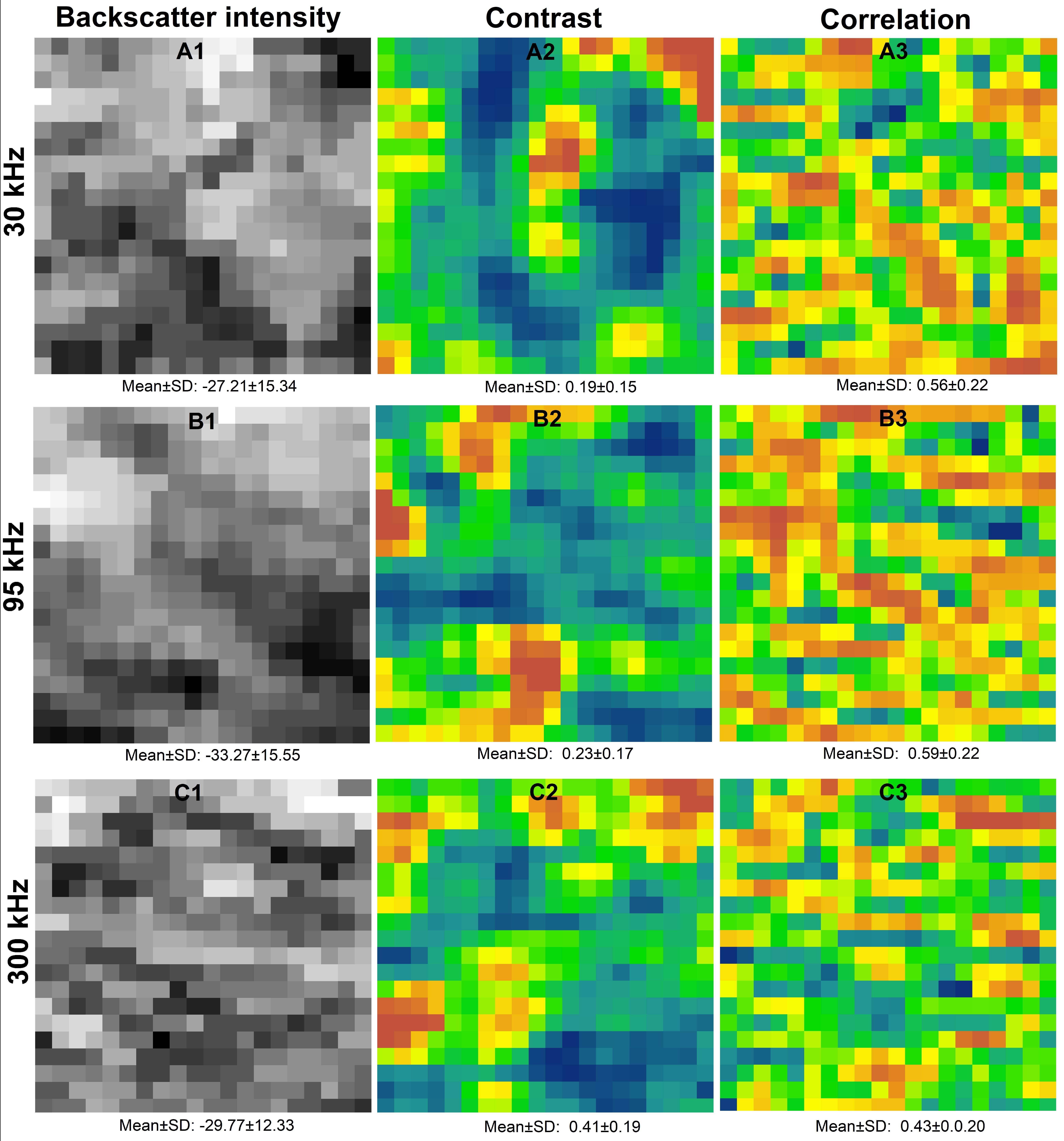
3.1.2. Texture-Based Acoustic Discrimination

A visual approach for discriminating the sediment grain size distribution (response variable) from the backscatter, contrast, and correlation as explanatory variables is given (Figure 6, Figure 7, Figure 8 and Figure 9). This visual approach pre-examined the relationship between backscatter and GLCM texture with sediments beyond single statistical parameter estimates like mean and median. The rasters showed fine scale variability in the texture intensity within and between frequencies for each sediment group. Variability was observed for backscatter and contrast GLCM features, while correlation had a rough texture with no clear pattern across all the frequencies and sediment classes. Generally, mean backscatter intensity was relatively higher for gravel than for all the other sediment classes, ranging between −17.82 ± 4.1 dB and −22.7 ± 11.79 dB at 300 kHz and 30 kHz, respectively (Figure 6). On the contrary, mean backscatter intensity was relatively lower for sand ranging between −33.27 ± 15.55 dB and −27.21 ± 15.34 dB for 95 kHz and 30 kHz, respectively. Meanwhile the contrast feature showed a slight variation in texture intensity between frequencies for the same sediment types, except for gravel (Figure 6, Figure 7, Figure 8 and Figure 9). For gravel, the texture intensity for contrast was between mean values of 0.19 ± 0.16 and 0.22 ± 1.9 for 30 kHz and 300 kHz, respectively (Figure 6). On the other hand, minimal variation in the mean values of the correlation feature was observed in all frequencies within and between sediment types (Figure 6, Figure 7, Figure 8 and Figure 9). These variations in texture were partly in harmony with the respective graphs of the sediment grain size distribution, which confirms the existence of backscatter–sediment relationships (Figure 6, Figure 7, Figure 8 and Figure 9).

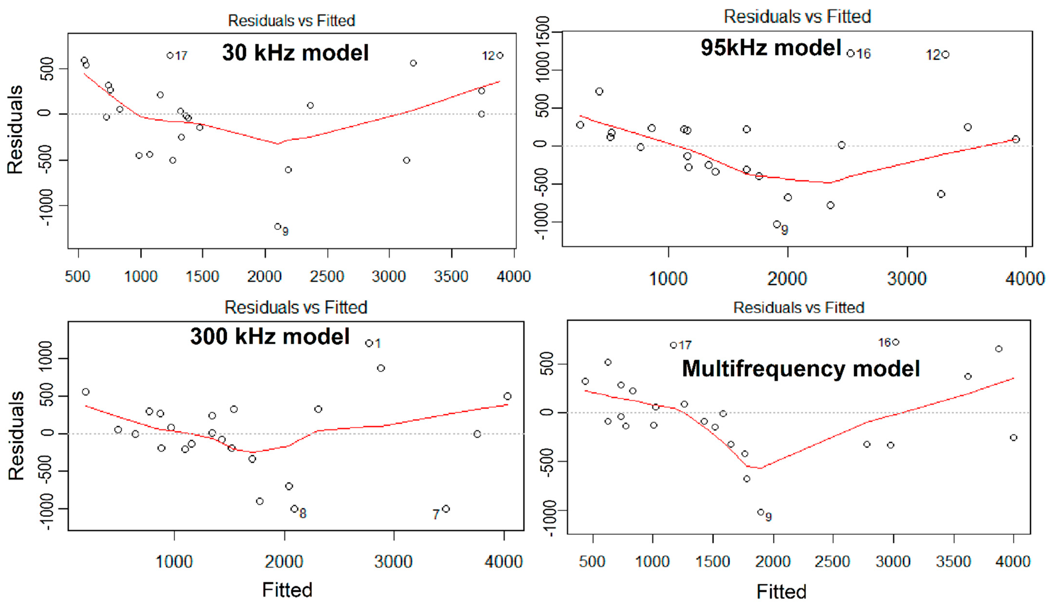
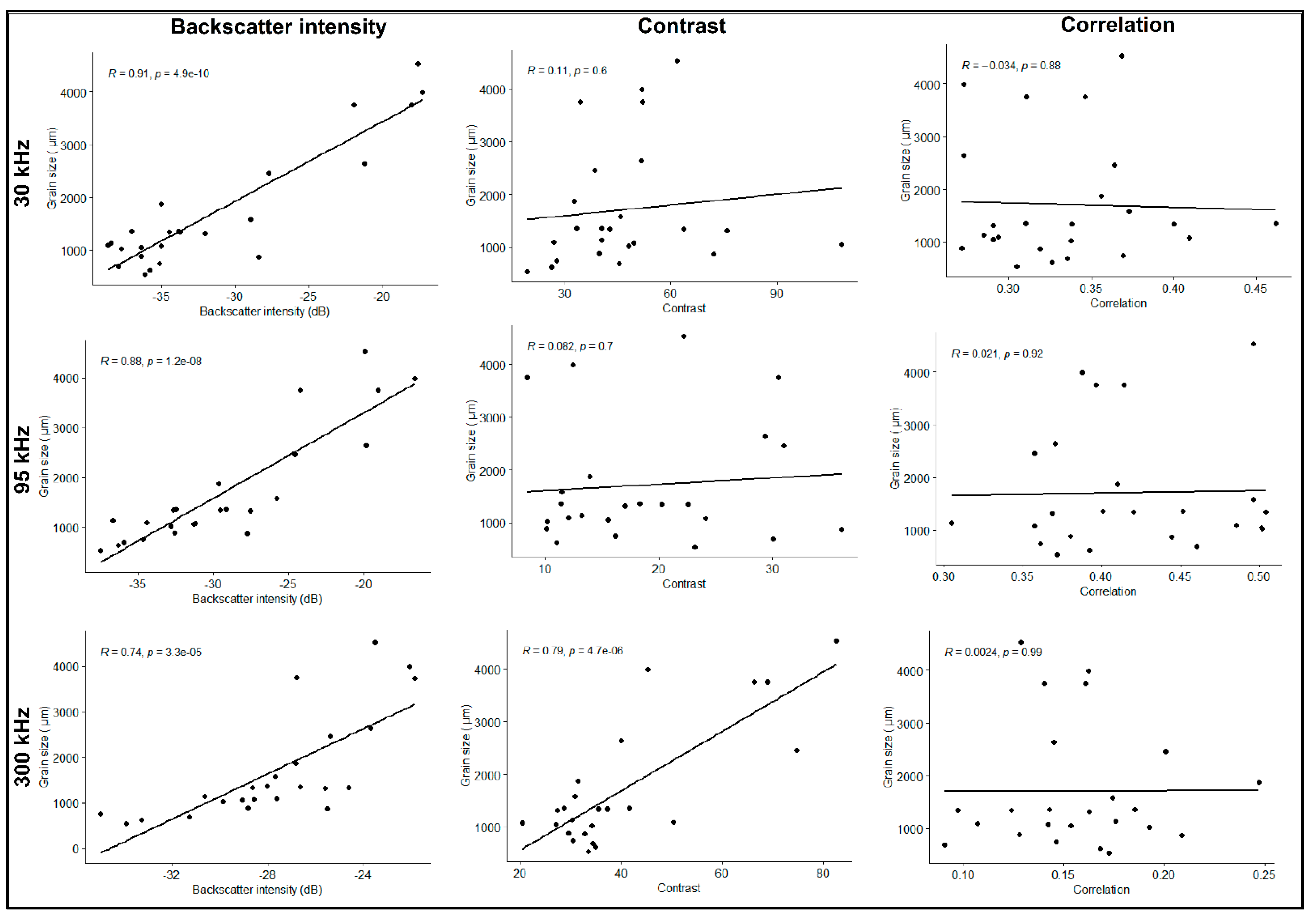
3.2. Modelling of Sediment Grain Size

First, we presented the results of Pearson’s correlation (ρ) between the mean sediment grain size and mean backscatter. The correlation between the mean backscatter and mean grain size was high for all the three frequencies (Figure A2). Mean backscatter at 30 kHz had the strongest correlation coefficient of 0.91 and was statistically significant at p < 0.05. This was followed by 95 kHz (ρ = 0.88), with the weakest correlation at 300 kHz (ρ = 0.74). Both were statistically significant with a p < 0.05. On the other hand, the statistical association between the selected texture features (contrast and correlation) and mean grain size was generally weak, and all results were statistically insignificant (p > 0.05), except for correlation (300 kHz), which had the strongest correlation coefficient of 0.79 (p < 0.05).

The 30 kHz model explained 84.3% (adjusted r² = 0.82) variability in the sediment grain size, followed closely by the 300 kHz model and 95 kHz model at 78.2% (adjusted r² = 0.75) and 78.0% (adjusted r² = 0.75), respectively. All the single-frequency models were statistically significant (p < 0.05). Lastly, the multifrequency model yielded a statistically significant output (p < 0.05) with 86.4% (adjusted r² = 0.84) variability. These results suggest that most of the variation was explained by the multifrequency model, whose output was more dominated by the 30 kHz data than the 300-kHz and 95-kHz models. Based on the RMSE values, the 30-kHz model had the lowest RMSE value at 545.2, meaning it performed relatively better than all the other models in terms of data fitting and performance. The multifrequency model at 545.8 was the next best, whereas for the 95-kHz model and 300-kHz models, with the highest RMSE values of 671.9 and 674.8, respectively, offered the lowest predictive capacity and performance.

The last part included the prediction of surficial sediments for each model, showing spatial variation in the sediment grain size using the model estimates shown in

Table 1. Summary results of the four generalized linear model (GLM) models presenting the model estimates and significance levels at p < 0.05 (with statistically significant variables denoted with asterisks) of the selected predictor variables. Mean backscatter and texture variables: contrast and correlation on the mean sediment grain size.

Covariates	Estimate	Std. Error	t-Value	p-Value
(1) 30 kHz model
Intercept	5862.7	892.2	6.6	0.000002 *
Backscatter	152.7	14.8	10.3	0.000000002 *
Contrast	−1.9	5.4	−0.3	0.7
Correlation	2220.0	2170.1	1.0	0.3
(2) 95 kHz model
Intercept	6712.5	1153.7	5.8	0.00001 *
Backscatter	172.2	20.6	8.4	0.00000006 *
Contrast	−4.1	15.4	−0.3	0.8
Correlation	276.7	2134.9	0.1	0.9
(3) 300 kHz model
Intercept	4280.6	1537.8	2.8	0.01 *
Backscatter	154.0	40.8	3.8	0.001 *
Contrast	39.8	8.7	4.6	0.0002 *
Correlation	552.5	3424.9	0.2	0.9
(4) Multifrequency model
Intercept	2465.8	757.7	3.3	0.004 *
Backscatter	577.0	83.5	6.9	0.000001 *
Contrast	26.2	10.7	2.4	0.02 *
Correlation	−4998.9	2392.9	−2.1	0.05

. A visible spatial pattern was observed between coarser and finer sediments, especially for the 30-kHz and 95-kHz models (Figure 10). Overall, finer sediments were more widespread than coarser sediments, especially in the central green-blue section of the 30-kHz and 95-kHz models (Figure 10). A closer inspection of the 500x500 m small area (within the red box) revealed that the 95 kHz and 30 kHz models distinguished an average grain size of 2.3 mm and 1.5 mm, respectively. In contrast, the 300 kHz and multifrequency models predicted a grain size of 1.3 mm and 1.2 mm in that order. Unknown here is the fine-scale bedform geometry, e.g., ripples that will change the grazing angles and cannot be separated from the surface scattering dependence on grain size.

4. Discussion

Traditionally, benthic habitat mapping has relied on single-frequency multibeam systems. However, with the improvement in sonar technology, multifrequency acoustic data acquisition is increasingly being used in recent studies [3,4,15]. The present study provides a robust framework with results highlighting the value of backscatter data acquired at multiple frequencies for characterising sediments in the range of coarse sand to gravel. We demonstrate the potential application of a combined approach to seafloor mapping and characterization, while underlining the value of optimizing the acquisition platforms and the reanalysis of existing legacy datasets.

4.1. Acoustic Discrimination of Sediments

Sediment properties have been used as abiotic proxies for seabed habitats [7,14]. Sediments determine the types of biological communities associated with benthic marine environments. Subsequently, these communities can impact on the total volume scattering acoustic responses of sediments [7,17]. However, direct quantification of geotechnical properties of the seafloor (e.g., grain size) is always a challenge. In this paper, we used sediment mean grain size as our response variable, and backscatter and GLCM features as our explanatory variables, an approach consistent with the literature [14,25].

Four main sediments’ classes (gravel, sandy gravel, gravelly sand, and sand) were identified based on the percentage proportion of grain size, with sand dominating the samples. The mixed sediments in this study area are characteristic of glaciated continental margins deposited by glacial processes and subsequently reworked by hydrodynamics. This type of mixed sediment dominates continental shelves in many areas of the Earth [36,52]. For researchers working in continental shelves, the mix of sediments has important applications for sensor choices for mapping in former glaciated margins vs. non-glaciated margins. The initial analysis demonstrated that the 30, 95, and 300 kHz responses varied widely when sediments changed from gravel to sand sediments. We show key thresholds for discriminating between gravel and mixed sand sediments ranging between −10 dB and −50 dB, with a higher acoustic signal recorded for gravel. The higher acoustic signal for hard and coarse-grained sediments is associated with a higher acoustic impedance contrast at the surface-water interface, subsequently returning a higher acoustic signature to the transducer, while finer sediments tend to scatter most of the signals away from the transducers [53]. In fact, a wider variability in backscatter responses between −15 dB and −45 dB for sandy sediments was captured for the lower frequency 30 kHz dataset, an observation which matches with the results of [7]. This initial finding provides evidence for the presence of a frequency-dependency component of backscatter influenced by both the interface and volume scattering regime [2,6,17,22]. The relatively higher backscatter responses for softer sediments has been linked to a strong volume scattering return [53], which depends on the penetration depth of the acoustic signal beyond the small bite depth (5–10cm) of the grab sample [2,8], and favours the lower frequency system (30 kHz). Furthermore, the lower frequency (30 kHz) has a better separation between gravelly and sandy sediments than the 95 kHz and 300 kHz datasets [2,9,17,54].

From our preliminary interpretations, all the sediment types across the three frequencies appeared slightly texturally dissimilar, with minimal variation within sediments (Figure 6, Figure 7, Figure 8 and Figure 9). The lower frequency (30 kHz) has a relatively higher textural intensity for backscatter than the 300 kHz, especially for sand. This exploration revealed more detail compared to the use of a single statistical measure of distribution (e.g., mean), which always masks out the fine scale variability. However, this high level of detail also rendered these small images to the influence of noise and size-specific texture sensitivity, hence caution needs to be exercised while interpreting the texture intensity [10,30,40].

4.2. Modelling Sediment Grain Size

Generally, a strong correlation exists between mean backscatter and mean grain size [14,24]. In contrast, the correlation between the individual texture features (contrast and correlation) and sediment grain size was generally weak and statistically insignificant (p > 0.05), suggesting that backscatter intensity is the most important predictor variable in this study. The poor performance of the GLCM texture can be linked to their sensitivity to survey geometry [30], analysis windows, distance between pixels, and the number of grey levels [10,27,40]. Similarly, the GLCM texture relies on pulse length and is unreliable at a high incidence angle [54]. Using only a selection of incidence angles while excluding the near-nadir and outer beams’ regions, and dealing with a single survey line, has been proposed as a solution to these limitations mentioned; especially when discriminating large seafloor features [30,40]. Nevertheless, several other studies that use a mosaic approach instead of portions of incidence angles exist [7,15,55].

For single frequency models, the 30 kHz models yielded a better statistical performance with adjusted r² values of 0.82 and explained the most variability (84.3%), compared with the 95 kHz and 300 kHz models. Our model evaluation based on RMSE values indicated that the 30 kHz data performed best, despite its originally intended purposes for deep-water mapping based on the limitations and caveats described in this study [56]. This highlights the additional value of low frequency swath systems in shallow water, providing an additional capacity for seafloor characterisation. From a processing perspective, the higher frequency (95 kHz and 300 kHz) data add little value to the model accuracy, and their inclusion present a burden in terms of processing power, data storage, and operational interferences during repeat acquisitions. However, these findings do not negate their multiple uses in other marine applications (e.g., hydrography and object detection); rather, they emphasize the value of using a combined approach to seafloor mapping and characterisation. In addition, the use of low frequency data could be a useful product to complement statutory mapping, even if it is outside the operational range of the system. All these highlight the value of maximising the acquisition platforms and the reanalysis of existing materials from legacy datasets.

While other studies have proposed acquisition of multifrequency backscatter from a single source [7,9,55], our study uses individual information from each single-frequency system to generate a multifrequency dataset using the PCA approach [39]. Multifrequency acquisition from a single source eliminates the potential problems associated with differences in sonar configuration, survey geometry, and signal penetration variation, which might influence the final output [2,17]. Our analysis shows negligible differences between the multifrequency model output and the 30 kHz model in terms of performance. This indicates that the 30 kHz data dominate the variance component of the multifrequency output, overshadowing the contribution of the 95 kHz and 300 kHz datasets. Generally, the results show a marginal gain of low single-frequency (30 kHz) data over higher frequency data (95 kHz and 300 kHz). However, the potential ability of low frequency systems to discriminate fine-scale geomorphology is low compared with higher frequency systems, and fully depends on the question under investigation. Visually, the predicted surfaces of the sediment grain size reveal that finer sediments are more widespread at the central section, especially for 30 kHz and 95 kHz models (Figure 10). The higher frequency (300 kHz) does not reflect as much variability compared with what is captured by the low frequency (30 kHz) model, and is likely dominated by reflection, making the sediments look texturally similar. This is in agreement with previous studies that indicate that acoustic maps based on single-frequency data may not always show the same parts of the seafloor because of the effect of depth and differences on signal penetration [2,9]. In addition, the poor performance of the 300 kHz model can be linked to the presence of the nadir response dominating the 300 kHz backscatter mosaic. Backscatter signal near the nadir region is highly variable and has minimal power to discriminate substrates [57]. In addition, the use of only 24 samples dominated by unconsolidated coarse sediments, and a possible greater signal penetration in favour of the lower frequency 30 kHz data [2,6,17], not only affects the reliability of the results, but also adds to the complexity in interpretation.

5. Limitations and Future Research

The major limitation of this study is the small sample size that was available to develop and validate our models. This is mainly because of the opportunistic analysis of existing datasets, and the physical difficulties of working in highly dynamic sea conditions (e.g., tides) and coarse sediments for granulometric analysis. Furthermore, combining datasets from multiple sources introduces additional complexities such as collinearity, noise, and lack of independence, which might not have been fully resolved in this study. Notwithstanding these limitations, the study offers a robust modelling framework, and in future, the presence of a large sample size would allow for some of these ideas to be tested in greater detail. In the future, we hope to further examine the frequency dependency component of backscatter to answer ecological questions by incorporating bathymetry, bathymetry derivatives, and biological data. All these variables have the potential to be included as inputs to seafloor classification and benthic habitat mapping to further augment the value of multifrequency MBES backscatter data for area-based monitoring and management in marine protected areas and other areas of the seabed.

6. Conclusions

The present study was designed to test the potential application of using multifrequency multibeam backscatter to predict sediment grain size. Visual analysis of the data enhances our understanding of the frequency variability of texture for different sediments, which are usually masked whenever measures of central tendency like mean and median values are used. The results of the study demonstrate a marginal gain of single low-frequency sources (30 kHz) over multifrequency analysis, which presents a burden in terms of processing power, data storage, and operational interferences during acquisition. This means that the use of a relatively low-frequency system initially designed for deep-water mapping might also be applicable in shallow water habitats or sediment discrimination, especially for former glaciated continental margins. However, the generalizability and wider application of these results require caution because they are site and installation specific, as the MBES systems used here lacked absolute calibration. Furthermore, they offer useful insights into the science community (e.g., GEOHAB) and may well have implications for other marine applications. We recommend that standardizing the acquisition and processing parameters of MBES data will have great benefits to multifrequency backscatter investigations. Moreover, with more availability of multifrequency backscatter data in the future, our ability to monitor and manage marine environments with similar geological and ecological settings will greatly be improved.

References

1. Cui, X.; Liu, H.; Fan, M.; Ai, B.; Ma, D.; Yang, F. Seafloor Habitat Mapping Using Multibeam Bathymetric and Backscatter Intensity Multi-Features SVM Classification Framework. Appl. Acoust. 2021, 174, 107728. [Google Scholar] [CrossRef]
2. Gaida, T.C.; Mohammadloo, T.H.; Snellen, M.; Simons, D.G. Mapping the Seabed and Shallow Subsurface with Multi-Frequency Multibeam Echosounders. Remote Sens. 2020, 12, 52. [Google Scholar] [CrossRef] [Green Version]
3. Lamarche, G.; Lurton, X. Recommendations for Improved and Coherent Acquisition and Processing of Backscatter Data from Seafloor-Mapping Sonars. Mar. Geophys. Res. 2018, 39, 5–22. [Google Scholar] [CrossRef] [Green Version]
4. Lecours, V.; Devillers, R.; Schneider, D.C.; Lucieer, V.L.; Brown, C.J.; Edinger, E.N. Spatial Scale and Geographic Context in Benthic Habitat Mapping: Review and Future Directions. MEPS 2015, 535, 259–284. [Google Scholar] [CrossRef] [Green Version]
5. Brown, C.J.; Smith, S.J.; Lawton, P.; Anderson, J.T. Benthic Habitat Mapping: A Review of Progress towards Improved Understanding of the Spatial Ecology of the Seafloor Using Acoustic Techniques. Estuar. Coast. Shelf Sci. 2011, 92, 502–520. [Google Scholar] [CrossRef]
6. Lurton, X.; Lamarche, G. Backscatter Measurements by Seafloor-mapping Sonars: Guidelines and Recommendations. In Geohab Report. 2015. Available online: https://niwa.co.nz/static/BWSG_REPORT_MAY2015_web.pdf (accessed on 15 January 2021).
7. Costa, B. Multispectral Acoustic Backscatter: How Useful Is It for Marine Habitat Mapping and Management? J. Coast. Res. 2019, 35, 1062. [Google Scholar] [CrossRef]
8. Feldens, P.; Schulze, I.; Papenmeier, S.; Schönke, M.; von Deimling, J.S. Improved Interpretation of Marine Sedimentary Environments Using Multi-Frequency Multibeam Backscatter Data. Geosciences 2018, 8, 214. [Google Scholar] [CrossRef]
9. Gaida, T.C.; Ali, T.A.T.; Snellen, M.; Amiri-Simkooei, A.; van Dijk, T.A.G.P.; Simons, D.G. A Multispectral Bayesian Classification Method for Increased Acoustic Discrimination of Seabed Sediments Using Multi-Frequency Multibeam Backscatter Data. Geosciences 2018, 8, 455. [Google Scholar] [CrossRef] [Green Version]
10. Huvenne, V.A.I.; Huhnerbach, V.; Blondel, P.; Gomez Sichi, O.; Le Bas, T. Detailed Mapping of Shallow-Water Environments Using Image Texture Analysis on Sidescan Sonar And Multibeam Backscatter Imagery. In Proceedings of the 2nd International Conference & Exhibition on “Underwater Acoustic Measurements: Technologies & Result”, Heraklion, Greece, 25–29 June 2007; pp. 879–886. [Google Scholar]
11. Boswarva, K.; Butters, A.; Fox, C.J.; Howe, J.A.; Narayanaswamy, B. Improving Marine Habitat Mapping Using High-Resolution Acoustic Data; A Predictive Habitat Map for the Firth of Lorn, Scotland. Cont. Shelf Res. 2018, 168, 39–47. [Google Scholar] [CrossRef]
12. Brown, C.; Beaudoin, J.; Brissette, M.; Gazzola, V. Setting the Stage for Multi-Spectral Acoustic Backscatter Research. In Proceedings of the United States Hydrographic Conference, Galveston, TX, USA, 26 September 2017. [Google Scholar]
13. Tamsett, D.; McIlvenny, J.; Watts, A. Colour Sonar: Multi-Frequency Sidescan Sonar Images of the Seabed in the Inner Sound of the Pentland Firth, Scotland. J. Mar. Sci. Eng. 2016, 4, 26. [Google Scholar] [CrossRef] [Green Version]
14. McGonigle, C.; Collier, J.S. Interlinking Backscatter, Grain Size and Benthic Community Structure. Estuar. Coast. Shelf Sci. 2014, 147, 123–136. [Google Scholar] [CrossRef]
15. Brown, C.J.; Beaudoin, J.; Brissette, M.; Gazzola, V. Multispectral Multibeam Echo Sounder Backscatter as a Tool for Improved Seafloor Characterization. Geosciences 2019, 9, 126. [Google Scholar] [CrossRef] [Green Version]
16. Fakiris, E.; Zoura, D.; Ramfos, A.; Spinos, E.; Georgiou, N.; Ferentinos, G.; Papatheodorou, G. Object-Based Classification of Sub-Bottom Profiling Data for Benthic Habitat Mapping. Comparison with Sidescan and RoxAnn in a Greek Shallow-Water Habitat. Estuar. Coast. Shelf Sci. 2018, 208, 219–234. [Google Scholar] [CrossRef]
17. Montereale-Gavazzi, G.; Roche, M.; Lurton, X.; Degrendele, K.; Terseleer, N.; Van Lancker, V. Seafloor Change Detection Using Multibeam Echosounder Backscatter: Case Study on the Belgian Part of the North Sea. Mar. Geophys. Res. 2018, 39, 229–247. [Google Scholar] [CrossRef]
18. Ierodiaconou, D.; Schimel, A.C.G.; Kennedy, D.; Monk, J.; Gaylard, G.; Young, M.; Diesing, M.; Rattray, A. Combining Pixel and Object Based Image Analysis of Ultra-High Resolution Multibeam Bathymetry and Backscatter for Habitat Mapping in Shallow Marine Waters. Mar. Geophys. Res. 2018, 39, 271–288. [Google Scholar] [CrossRef]
19. Kirui, K.B.; Kairo, J.G.; Bosire, J.; Viergever, K.M.; Rudra, S.; Huxham, M.; Briers, R.A. Mapping of Mangrove Forest Land Cover Change along the Kenya Coastline Using Landsat Imagery. Ocean Coast. Manag. 2013, 83, 19–24. [Google Scholar] [CrossRef]
20. Dahdouh-guebas, F. The use of remote sensing and gis in the sustainable management of tropical coastal ecosystems each of these habitats is formed by species that are to a large extent adapted to trop-intertidal forests that are composed of halotolerant plant species. Environ. Dev. Sustain. 2002, 4, 93–112. [Google Scholar] [CrossRef] [Green Version]
21. Ruddick, K.; Neukermans, G.; Vanhellemont, Q.; Jolivet, D. Challenges and Opportunities for Geostationary Ocean Colour Remote Sensing of Regional Seas: A Review of Recent Results. Remote Sens. Environ. 2014, 146, 63–76. [Google Scholar] [CrossRef] [Green Version]
22. Lacharité, M.; Brown, C.J.; Gazzola, V. Multisource Multibeam Backscatter Data: Developing a Strategy for the Production of Benthic Habitat Maps Using Semi-Automated Seafloor Classification Methods. Mar. Geophys. Res. 2018, 39, 307–322. [Google Scholar] [CrossRef]
23. Buscombe, D.; Grams, P.E.; Kaplinski, M.A. Compositional Signatures in Acoustic Backscatter Over Vegetated and Unvegetated Mixed Sand-Gravel Riverbeds. J. Geophys. Res. Earth Surf. 2017, 122, 1771–1793. [Google Scholar] [CrossRef] [Green Version]
24. Brown, C.J.; Collier, J.S. Mapping Benthic Habitat in Regions of Gradational Substrata: An Automated Approach Utilising Geophysical, Geological, and Biological Relationships. Estuar. Coast. Shelf Sci. 2008, 78, 203–214. [Google Scholar] [CrossRef]
25. Collier, J.S.; Brown, C.J. Correlation of Sidescan Backscatter with Grain Size Distribution of Surficial Seabed Sediments. Mar. Geol. 2005, 214, 431–449. [Google Scholar] [CrossRef]
26. Lucieer, V.; Hill, N.A.; Barrett, N.S.; Nichol, S. Do Marine Substrates “look” and “Sound” the Same? Supervised Classification of Multibeam Acoustic Data Using Autonomous Underwater Vehicle Images. Estuar. Coast. Shelf Sci. 2013, 117, 94–106. [Google Scholar] [CrossRef]
27. Janowski, A.; Tȩgowski, J.; Nowak, J. Seafloor Mapping Based on Multibeam Echosounder Bathymetry and Backscatter Data Using Object-Based Image Analysis: A Case Study from the Rewal Site, the Southern Baltic. Oceanol. Hydrobiol. Stud. 2018, 47, 248–259. [Google Scholar] [CrossRef]
28. Buscombe, D.; Grams, P.E. Probabilistic Substrate Classification with Multispectral Acoustic Backscatter: A Comparison of Discriminative and Generative Models. Geosciences 2018, 8, 395. [Google Scholar] [CrossRef] [Green Version]
29. Fakiris, E.; Blondel, P.; Papatheodorou, G.; Christodoulou, D.; Dimas, X.; Georgiou, N.; Kordella, S.; Dimitriadis, C.; Rzhanov, Y.; Geraga, M.; et al. Multi-Frequency, Multi-Sonar Mapping of Shallow Habitats-Efficacy and Management Implications in the National Marine Park of Zakynthos, Greece. Remote Sens. 2019, 11, 461. [Google Scholar] [CrossRef] [Green Version]
30. Feldens, P.; Survey, A.H. Sensitivity of Texture Parameters to Acoustic Incidence Angle in Multibeam Backscatter. IEEE Geosci. Remote Sens. Lett. 2017, 14, 2215–2219. [Google Scholar] [CrossRef]
31. MARPAMM. Marine Protected Area Management & Monitoring. Available online: https://www.mpa-management.eu/ (accessed on 19 December 2020).
32. Long, D. BGS Detailed Explanation of Seabed Sediment Modified Folk Classification; MESH Report; Joint Nature Conservation Committee: Peterborough, UK, 2006. [Google Scholar]
33. Evans, W. Hydrodynamic Modelling of Sediment Transport and Bedform Formation on the NW Irish Shelf. Ph.D. Thesis, Ulster University, Coleraine, UK, 2018. [Google Scholar]
34. Picton, B.; Costello, M.J. BioMar Biotope Viewer: A Guide to Marine Habitats, Fauna and Flora of Britain and Ireland; Environmental Sciences Unit Trinity College: Dublin, UK, 1998; ISBN 0 9526 735 4. [Google Scholar]
35. NPWS. Hempton’s Turbot Bank SAC (Site Code: 2999) Conservation Objectives Supporting Document—Marine Habitats; Version 1; 2015. Available online: https://www.npws.ie/protected-sites/sac/002999 (accessed on 15 March 2021).
36. Evans, W.; Benetti, S.; Sacchetti, F.; Jackson, D.W.T.; Dunlop, P.; Monteys, X. Bedforms on the Northwest Irish Shelf: Indication of Modern Active Sediment Transport and over Printing of Paleo-Glacial Sedimentary Deposits. J. Maps 2015, 11, 561–574. [Google Scholar] [CrossRef] [Green Version]
37. Williams, J.J.; MacDonald, N.J.; O’Connor, B.A.; Pan, S. Offshore Sand Bank Dynamics. J. Mar. Syst. 2000, 24, 153–173. [Google Scholar] [CrossRef]
38. Simpson, J.H.; Allen, C.M.; Morris, N.C.G. Fronts on the Continental Shelf. J. Geophys. Res. 1978, 83, 4607–4614. [Google Scholar] [CrossRef]
39. Kupidura, P. The Comparison of Different Methods of Texture Analysis for Their Efficacy for Land Use Classification in Satellite Imagery. Remote Sens. 2019, 11, 1233. [Google Scholar] [CrossRef] [Green Version]
40. Febriawan, H.K.; Helmholz, P.; Parnum, I.M. Support Vector Machine and Decision Tree Based Classification of Side-Scan Sonar Mosaics Using Textural Features. Int. Arch. Photogramm. Remote Sens. Spat. Inf. Sci. ISPRS Arch. 2019, 42, 27–34. [Google Scholar] [CrossRef] [Green Version]
41. Haralick, M.R.; Shanmugam, K.; Dinstein, I. Textural Features for Image Classification. IEEE Trans. Syst. Man Cybern. 1973, 6, 610–621. [Google Scholar] [CrossRef] [Green Version]
42. Clausi, D.A. An Analysis of Co-Occurence Texture Statistics as a Function of Grey Level Quantization. Can. J. Remote Sens. 2002, 28, 45–62. [Google Scholar] [CrossRef]
43. Zuur, A.F.; Ieno, E.N.; Elphick, C.S. A Protocol for Data Exploration to Avoid Common Statistical Problems. Methods Ecol. Evol. 2010, 1, 3–14. [Google Scholar] [CrossRef]
44. Price, D.M.; Robert, K.; Callaway, A.; Lo lacono, C.; Hall, R.A.; Huvenne, V.A.I. Using 3D Photogrammetry from ROV Video to Quantify Cold-Water Coral Reef Structural Complexity and Investigate Its Influence on Biodiversity and Community Assemblage. Coral Reefs 2019, 38, 1007–1021. [Google Scholar] [CrossRef] [Green Version]
45. O’Fallon, W.M.; Cooley, W.W.; Lohnes, P.R. Multivariate Data Analysis. Technometrics 1973, 15, 648. [Google Scholar] [CrossRef]
46. Reiss, H.; Cunze, H.; König, K.; Neumann, K.; Kröncke, I. Species Distribution Modelling of Marine Benthos: A North Sea Case Study. MEPS 2011, 442, 71–86. [Google Scholar] [CrossRef] [Green Version]
47. Fournier, A.; Barbet-Massin, M.; Rome, Q.; Courchamp, F. Predicting Species Distribution Combining Multi-Scale Drivers. GECCO 2017, 12, 215–226. [Google Scholar] [CrossRef]
48. Trzcinska, K.; Janowski, L.; Nowak, J.; Rucinska-Zjadacz, M.; Kruss, A.; von Deimling, J.S.; Pocwiardowski, P.; Tegowski, J. Spectral Features of Dual-Frequency Multibeam Echosounder Data for Benthic Habitat Mapping. Mar. Geol. 2020, 427, 106239. [Google Scholar] [CrossRef]
49. Izzo, G.; Jackiewicz, Z. Generalized Linear Multistep Methods for Ordinary Differential Equations. Appl. Numer. Math. 2017, 114, 165–178. [Google Scholar] [CrossRef]
50. Koc, E.K.; Bozdogan, H. Model Selection in Multivariate Adaptive Regression Splines (MARS) Using Information Complexity as the Fitness Function. Mach. Learn. 2015, 101, 35–58. [Google Scholar] [CrossRef]
51. Casal, G.; Harris, P.; Monteys, X.; Hedley, J.; Cahalane, C.; McCarthy, T. Understanding Satellite-Derived Bathymetry Using Sentinel 2 Imagery and Spatial Prediction Models. GIScience Remote Sens. 2020, 57, 271–286. [Google Scholar] [CrossRef]
52. Sacchetti, F.; Benetti, S.; Georgiopoulou, A.; Shannon, P.M.; O’Reilly, B.M.; Dunlop, P.; Quinn, R.; Cofaigh, C.Ó. Deep-Water Geomorphology of the Glaciated Irish Margin from High-Resolution Marine Geophysical Data. Mar. Geol. 2012, 291–294, 113–131. [Google Scholar] [CrossRef]
53. Huang, Z.; Siwabessy, J.; Cheng, H.; Nichol, S. Using Multibeam Backscatter Data to Investigate Sediment-Acoustic Relationships. J. Geophys. Res. Oceans 2018, 123, 4649–4665. [Google Scholar] [CrossRef]
54. Clarke, J.E.H. Multispectral Acoustic Backscatter from Multibeam, Improved Classification Potential. In Proceedings of the United States Hydrographic Conference, San Diego, CA, USA, 16–19 March 2015; pp. 15–19. [Google Scholar]
55. Misiuk, B.; Brown, C.J.; Robert, K. Harmonizing Multi-Source Sonar Backscatter Datasets for Seabed Mapping Using Bulk Shift Approaches. Remote Sens. 2020, 12, 601. [Google Scholar] [CrossRef] [Green Version]
56. Misiuk, B.; Diesing, M.; Aitken, A.; Brown, C.J.; Edinger, E.N.; Bell, T. A Spatially Explicit Comparison of Quantitative and Categorical Modelling Approaches for Mapping Seabed Sediments Using Random Forest. Geosciences 2019, 9, 254. [Google Scholar] [CrossRef] [Green Version]
57. Gaida, T.C.; Snellen, M.; van Dijk, T.A.G.P.; Simons, D.G. Geostatistical Modelling of Multibeam Backscatter for Full-Coverage Seabed Sediment Maps. Hydrobiologia 2019, 845, 55–79. [Google Scholar] [CrossRef] [Green Version]
Figure 1. Locations of Hempton’s Turbot Bank special area of conservation (SAC) and Marine Protected Area Monitoring and Management (MarPAMM) project domain areas of the North Atlantic Ocean (Bathymetry source: GEBCO, 2019).
Remotesensing 13 01539 g001
Figure 2. (A) Bathymetric variation at Hempton’s Turbot Bank SAC. (B) Sediment grain size data (Folk classification) superimposed on the 30 kHz backscatter mosaic. The red bounding polygon shows the common analysis extent covered by 30, 95, and 300-kHz backscatter mosaics.
Remotesensing 13 01539 g002
Figure 3. Single frequency backscatter mosaics; (AC) representing 30, 95, and 300 kHz, respectively; (D) multifrequency backscatter mosaic and a range of eight surfaces produced from the grey level co-occurrence matrix (GLCM) analysis on the 30 kHz backscatter. CO—contrast; CC—correlation; DI—dissimilarity; EN—entropy; HO—homogeneity; ME—mean; SM—second moment; VA—variance. The colour ramps for the GLCM surfaces are based on a common scheme adjusted to the second order standard deviation to accentuate the features in the data and are scaled between 1 (high) and 0 (low) texture intensities.
Remotesensing 13 01539 g003
Figure 4. The developed workflow showing the feature extraction, selection, and data analysis as used in this study.
Remotesensing 13 01539 g004
Figure 5. Distribution of relative backscatter intensities for different sediment classes across the three operating frequencies, represented as (A) 30 kHz, (B) 95 kHz, and (C) 300 kHz. The sediment classes are represented as dark pink, pink, yellow, and mango for gravel (1, 11, and 12), sandy gravel (7, 10, 16, and 17), gravelly sand (13, 18, 19, 21,22, and 23), and sand (2, 3, 4, 5, 6, 8, 9, 14, 15, 20, and 24), respectively, classified under the Folk sediment classification scheme (triangle).
Remotesensing 13 01539 g005
Figure 6. Multipanel plot showing the visual comparison of the textural intensity for the backscatters and their GLCM texture derivatives for station 12, representing the gravel class.
Remotesensing 13 01539 g006
Figure 7. Multipanel plot showing the visual comparison of the textural intensity for the backscatters and their GLCM texture derivatives for station 10, representing the sandy gravel class.
Remotesensing 13 01539 g007
Figure 8. Multipanel plot showing a visual comparison of the textural intensity for the backscatters and their GLCM texture derivatives for station 13, representing the gravelly sand class.
Remotesensing 13 01539 g008
Figure 9. Multipanel plot showing a visual comparison of the textural intensity for backscatter and their GLCM texture derivatives for station 15 representing the sand class.
Remotesensing 13 01539 g009
Figure 10. Prediction of surficial sediment grain size from GLM. The following four models are shown and compared: 30 kHz model, 95 kHz model, 300 kHz model, and the multifrequency model with the 500x500 m small areas (red polygons), showing subtle variation in mean sediment grain size. The values are rescaled between 1 μm (clay/silt) and 120,000 μm (cobbles), and standard deviation stretching is applied on a colour ramp to accentuate features. The specific grain size classes for different sediment types are as follows: cobble (64,000–120,000 μm), pebble (4000–64,000 μm), granule (2000–4000 μm), very coarse sand (1000–2000 μm), coarse sand (500–1,000 μm), medium sand (250–500 μm), fine sand (125–250 μm), very fine sand (62.5–125 μm), and clay/silt (≤ 62.5 μm).
Remotesensing 13 01539 g010