Article

The Use of Sentinel-2 for Chlorophyll-a Spatial Dynamics Assessment: A Comparative Study on Different Lakes in Northern Germany

1
Department of Experimental Limnology, Leibniz Institute of Freshwater Ecology and Inland Fisheries, Zur alten Fischerhuette 2, 16775 Stechlin, Germany
2
Department of Ecohydrology, Leibniz Institute of Freshwater Ecology and Inland Fisheries, Müggelseedamm 310, 12587 Berlin, Germany
3
Remote Sensing and Geoinformatics, GFZ German Research Centre for Geosciences, Telegrafenberg, 14473 Potsdam, Germany
4
Institute for Space Sciences, Freie Universität Berlin, Carl-Heinrich-Becker Weg 6-10, 12165 Berlin, Germany
5
Faculty of Mathematics and Natural Sciences, Potsdam University, Maulbeerallee 2, 14469 Potsdam, Germany
*
Author to whom correspondence should be addressed.
Submission received: 10 March 2021 / Revised: 8 April 2021 / Accepted: 13 April 2021 / Published: 16 April 2021
(This article belongs to the Special Issue Remote Sensing of Aquatic Ecosystem Health and Processes)

Abstract

:
Eutrophication of inland waters is an environmental issue that is becoming more common with climatic variability. Monitoring of this aquatic problem is commonly based on the chlorophyll-a concentration monitored by routine sampling with limited temporal and spatial coverage. Remote sensing data can be used to improve monitoring, especially after the launch of the MultiSpectral Instrument (MSI) on Sentinel-2. In this study, we compared the estimation of chlorophyll-a (chl-a) from different bio-optical algorithms using hyperspectral proximal remote sensing measurements, from simulated MSI responses and from an MSI image. For the satellite image, we also compare different atmospheric corrections routines before the comparison of different bio-optical algorithms. We used in situ data collected in 2019 from 97 sampling points across 19 different lakes. The atmospheric correction assessment showed that the performances of the routines varied for each spectral band. Therefore, we selected C2X, which performed best for bands 4 (root mean square error—RMSE = 0.003), 5 (RMSE = 0.004) and 6 (RMSE = 0.002), which are usually used for the estimation of chl-a. Considering all samples from the 19 lakes, the best performing chl-a algorithm and calibration achieved a RMSE of 16.97 mg/m3. When we consider only one lake chain composed of meso-to-eutrophic lakes, the performance improved (RMSE: 10.97 mg/m3). This shows that for the studied meso-to-eutrophic waters, we can reliably estimate chl-a concentration, whereas for oligotrophic waters, further research is needed. The assessment of chl-a from space allows us to assess spatial dynamics of the environment, which can be important for the management of water resources. However, to have an accurate product, similar optical water types are important for the overall performance of the bio-optical algorithm.

Graphical Abstract

1. Introduction

Inland water bodies comprise large networks of geographically distributed hydrologic freshwater ecosystems, which integrate their surrounding terrestrial area and are sites of intense biogeochemical activity [1]. They are sentinel systems for the response of the entire watershed to climate variation [2]. Furthermore, inland water bodies provide many ecosystem services to humans, including drinking water, food, transport, energy, industrial purposes and recreation [3]. However, anthropogenic pressure on aquatic systems often results in water quality degradation [4]. A major challenge regarding inland waters is increasing eutrophication [5], which can be detected through enhanced chlorophyll-a (chl-a) concentration, a proxy for trophic state [6]. Chl-a is the pigment that all phytoplankton species have in common [7] and the primary optically active component used when studying water color [8]. Traditional water quality monitoring programs involve field sampling and laboratory analysis, which are time-consuming, costly, and not always feasible [9]. Recently, buoys equipped with automated multiparameter probes have been used to increase the frequency of data acquisition [10,11] and reduce laboratory-based analysis. However, neither laboratory- nor probe-based water quality assessments can readily capture the spatial heterogeneity combined with the temporal dynamics of water quality [12]. To quantify these dynamics, remote sensing techniques have been developed to monitor proxies for water quality parameters, including chl-a ([8,13,14]) and water transparency [15,16] in inland water systems. The advantages of using remote sensing techniques to monitor water quality are (1) the huge spatial coverage of satellite images, which provide information from a large area opposed to few or single point sampling location(s), (2) the ability to obtain information from inaccessible water bodies, (3) the ability to retrieve historical data from past satellite images [17] and (4) fast assessment of the ecological status of water quality compared to some laboratory techniques [16]. Given appropriate weather conditions, current remote sensing techniques are useful tools for water quality monitoring, enabling a time-saving and cost-effective water resource management [12].
One of the main challenges for current remote sensing of water quality is the spatial resolution of the sensors to detect useful optical information from lakes, which cover 3.7% of the Earth’s nonglaciated land area [18]. However, the number of small lakes is much higher than the number of large lakes [19]. Traditional ocean color sensors such as the Moderate Resolution Imaging Spectroradiometer (MODIS), the Medium Resolution Imaging Spectrometer (MERIS) and the Ocean and Land Colour Instrument (OLCI) onboard of Sentinel-3 have a low spatial resolution compared to land observation sensors [20]. Satellites with higher spatial resolution, like the Landsat satellite family, lack important spectral bands for the estimation of water quality parameters, such as the narrow absorption spectral feature of chl-a around 665 nm. With the launch of the MultiSpectral Instrument (MSI) onboard Sentinel-2 satellites (A and B, launched in 2015 and 2017, respectively), a new opportunity to explore smaller aquatic systems (larger than 100 m2) appeared. Although the MSI was not designed for aquatic remote sensing, its spatial resolution of down to 10–20 m per pixel is suitable for aquatic systems of 900 m2 and its spectral resolution is appropriate for detecting the chl-a absorption peak at 665 nm and the backscattering of particles at 705 nm [21].
An important challenge for water quality remote sensing is the atmospheric correction for satellite imagery over inland waters [22]. For optically complex inland waters, this task is complicated due to additional effects such as water turbidity, which can increase the signal in the near-infrared spectrum, whitecaps, sun glint and adjacency effects from the surrounding land [23]. Therefore, for the computation of the remote sensing reflectance (Rrs), atmospheric correction is a key processing step to lake color remote sensing [24].
The first study to investigate the use of Sentinel-2 for the monitoring of inland water quality parameters was conducted in two eutrophic lakes: Lake Peipsi and Lake Võrtsjärv, both located in Estonia [20]. Chl-a was estimated based on the peak height at 705 nm (band 5), which was calculated against band 4 (665 nm) and band 6 (740 nm) baselines with a coefficient of determination (R2) of 0.80. The authors recommend using an algorithm relying on red-near-infrared spectral bands, especially in lakes with high organic matter concentrations, causing high absorption of short wavelength radiation. However, the use of band 6 can be compromised by adjacency effects. Another study estimated chl-a concentration by testing different combinations of band ratios and correlating them to chl-a concentrations samples from the tropical mesotrophic Lake Ba Be (Vietnam) [25]. The authors found that the best band ratio for the estimation of chl-a concentration was the green–red band ratio with an R2 of 0.68. Overall, this study was based on empirical relationships that are difficult to replicate in other systems. The use of Sentinel-2 imagery was also evaluated for the estimation of chl-a in subalpine lakes in Italy, which are mostly oligotrophic with few meso-to-eutrophic lakes [26], using the Bio-Optical Model-Based tool for Estimating water quality and bottom properties from Remote sensing images (BOMBER) [27]. Different from previous studies, which used empirical and semiempirical approaches for estimating chl-a concentration, BOMBER used a physical approach for the monitoring of water quality with Sentinel-2 imagery. For chl-a estimation, the model is based on the spectral inversion procedure, where the specific absorption spectra of phytoplankton are used for the calculation of the chl-a concentration (R2 = 0.82). Recently, Li et al. [28] proposed a machine learning method for the estimation of chl-a concentration from Sentinel-2 imagery in 45 Chinese lakes with trophy varying from oligotrophic to hypertrophic. The authors created three clusters of Rrs and identified the best machine learning algorithms by testing linear regression model, support vector machine model and Catboost model for the estimation of chl-a and other water quality parameters for each cluster (R2 = 0.50, 0.64 and 0.79 for clusters 1, 2 and 3). While the use of machine learning approaches is increasing, the need of large training data sets is important to improve the performance. In another study from 10 mesotrophic Estonian lakes, chl-a concentration was computed based on semiempirical algorithms from the literature and showed that the performance of an algorithm varied from lake to lake [29]. This highlights the need of an algorithm that can be geographically transferable and the need to understand the optical properties of the lakes being monitored, which can be related to the trophy state of the aquatic system. Thus, for the oligotrophic waters in subalpine lakes in Italy, a physical approach was more adequate [26], whereas for meso-to-eutrophic waters, band ratios were used [20,25,29].
In terms of atmospheric correction, the first study using Sentinel-2 images [20] computed the bottom of the atmosphere reflectance estimated by the standard atmospheric correction routine for Sentinel-2. However, the study did not have simultaneous field radiometry data to validate the atmospheric correction performance. In the study at Lake Ba Be (Vietnam) [25], Sentinel-2 images were atmospherically corrected using an empirical line, which is a technique that only allows the correction for that specific Sentinel 2/MSI scene. Nevertheless, the authors applied the same empirical line to other scenes over the same area in different months and years. In the Italian subalpine lakes, Sentinel-2 images were atmospherically corrected by the Second Simulation of the Satellite Signal in the Solar Spectrum (6S) atmospheric correction [26]. The authors evaluated the 6S atmospheric correction routine for bands 1, 2, 3 and 4 and showed that there was an overestimation for these four spectral bands. Unfortunately, bands 5 and 6 were not evaluated. For the study in 45 Chinese lakes, authors did not evaluate the atmospheric correction which was made by the Case-2 Regional Coast Colour (C2RCC). While the studies mentioned above used only one atmospheric correction routine and a specific method for estimating chl-a, a study from 10 Estonian lakes evaluated the performance of four different atmospheric correction routines of which three were developed for inland waters. In that study, the C2RCC processor showed the best performance; however, authors observed that it was not sensitive in estimating band 4, which is crucial for chl-a estimation [29]. This issue was later fixed by the inclusion of the extreme case look-up tables via the Case-2 Extreme Cases (C2X) atmospheric correction routine, which is an extension of the C2RCC.
Based on previous research, we noticed a lack of atmospheric correction assessments when evaluating the use of Sentinel 2/MSI imagery for chl-a concentration estimation. Therefore, in this study, we tried to not only assess the most suitable chl-a algorithm but also the best atmospheric correction routine. The primary goal of our study was to assess the spatial heterogeneity of chl-a from relatively small (0.8–5.1 km2) oligo- to polytrophic lakes in Northern Germany from Sentinel-2/MSI images. To do that, we present the measurements and methodologies used to assess the best atmospheric correction routine and bio-optical algorithm for our study site (Section 2). In Section 3, we present the results of our comparison among six different atmospheric corrections routines and five bio-optical algorithms with different calibrations. We discuss our results in Section 4, comparing them with previous studies as well as discussing the spatial heterogeneity of chl-a and its use for environmental management. Finally, Section 5 presents the summary of the study as well as some future directions.

2. Materials and Methods
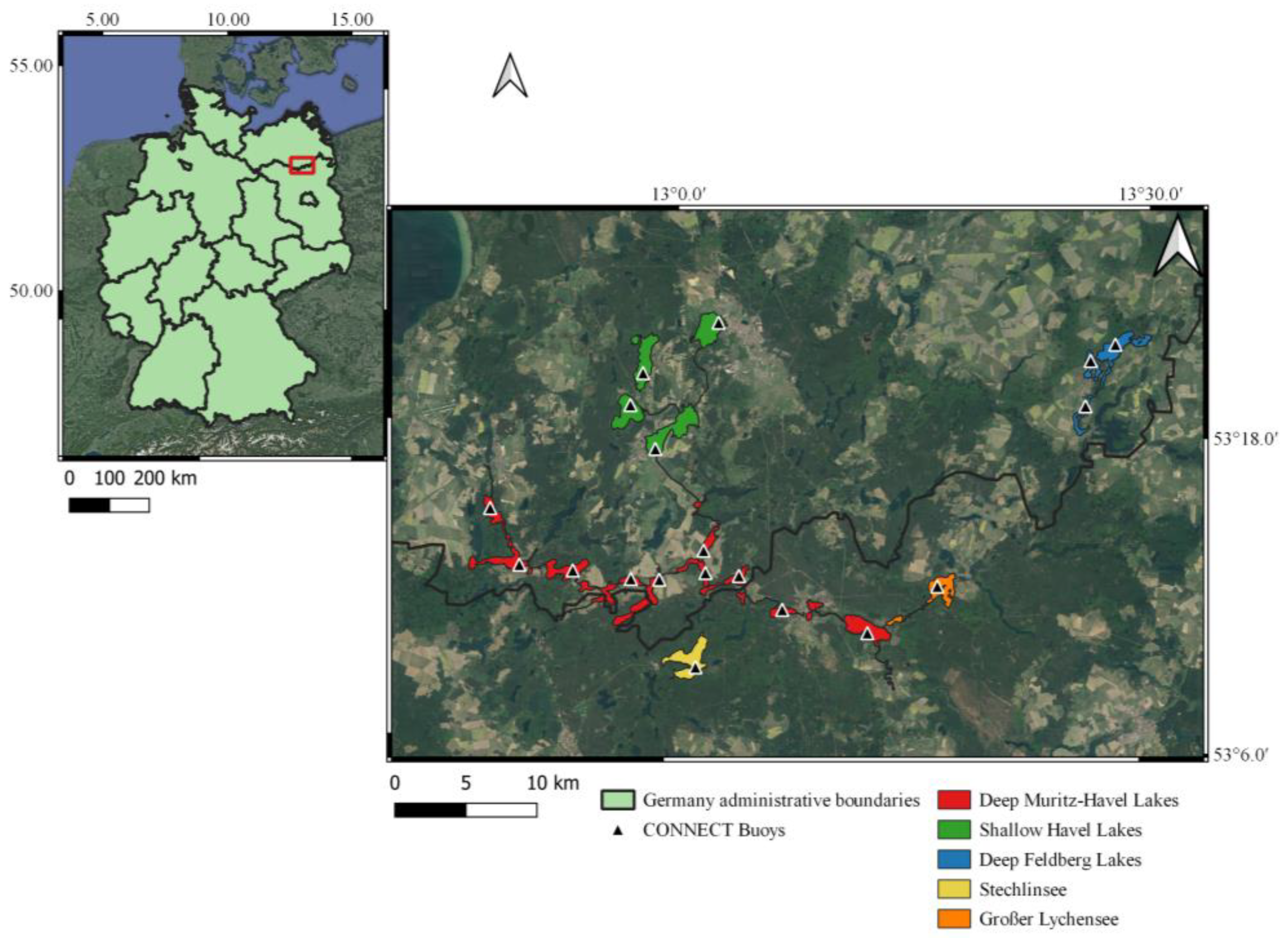
2.1. Study Site

The Mecklenburg–Brandenburg lake district encompasses more than 1000 lakes and is situated in the glacially formed North German Lowland. The studied lakes are located about 100 km north of Berlin (Figure 1). The lakes within this area cover various sizes, shapes, depths and a wide range in trophic state and biogeochemical characteristics (Table 1) [30]. Several of these lakes have been previously measured by the European Multi Lake Survey (EMLS) [31], which confirms the diversity in the biogeochemical characterization observed in the early 2000s. Moreover, many of the lakes are connected by rivers, streams and natural or manmade channels and provide regionally important ecosystem services especially for transportation, professional and sports fisheries, as well as other recreation and sports activities. This study region is, therefore, of high interest for monitoring and management and offers a unique possibility to study river-connected lake systems in the North German Lowland.
In this study, we collected data from 19 lakes, which we divided into four groups: Deep Müritz-Havel Lakes (from West to East, Zotzensee, Vilzsee, Labussee, Kleiner Pälitzsee, Groβer Pälitzsee, Ellbogensee, Groβer Priepertsee, Ziernsee, Röblinsee and Stolpsee), Shallow Havel Lakes (from North to South, Zierker See, Useriner See, Groβer Labussee and Woblitzsee, although the Zierker See is not exactly located at the Upper Havel River path), individual lakes (Großer Lychensee and Stechlinsee) and the Deep Feldberg Lakes (from West to East, Schmaler Luzin, Feldberger Haussee, and Breiter Luzin), as shown in Figure 1.
The Shallow Havel Lakes are connected to each other via the Upper Havel river system flowing southward and finally merge with the Deep Müritz-Havel Lakes at the northern end of Ellbogensee. Großer Lychensee is also connected to the Deep Müritz-Havel Lakes via Stolpsee and the River Woblitz. The Deep Feldberg Lakes are connected to each other, but without any further river connection to other lakes, and Lake Stechlin is fully disconnected from the other study lakes. All these lakes have been previously classified using the trophic index (classification system designed to rate water bodies based on the amount of biological productivity) of the German working group on water issues (LAWA) [32] giving index values between 1.4 and 3.7, which correspond to the range of oligotrophic to hypereutrophic waters (Table 1). The Deep Müritz-Havel Lakes are more connected among them, followed by the Shallow Havel Lakes, and lastly the individual lakes (Großer Lychensee and Stechlinsee) and the Deep Feldberg Lakes.

2.2. In Situ Data Set

All in situ data were collected during six field campaigns conducted between June and October 2019. Unfortunately, only the campaign conducted on 26 July 2019 had cloud-free sky and coincided with a Sentinel-2A/MSI passage over the area of interest. The Sentinel-2A/MSI Level-1 image (Scene ID: GS2A_20190726T102031_021369_N02.08) was downloaded from Copernicus Open Access Hub (scihub.copernicus.eu). We collected the water samples from 1 m depth and above water radiometric data at the previously installed buoys as part of the CONNECT Project (see Figure 1, buoy coordinates according to Table 1). On 26 July 2019, we used the opportunity of clear sky and the passage of a Sentinel-2A/MSI to conduct an extra campaign with several sampling points per lake on a subset of the study lakes, namely, the lakes Ellbogensee, Großer Priepertsee, Labussee, Vilzsee, Ziernsee and Zotzensee. In this campaign, we retrieved a total of 32 sampling points collected in areas without bottom reflectance and far from the shoreline of these lakes. The location of the individual sampling points for this field campaign can be found in Ogashawara et al. [34]. The total in situ data set used in this study encompasses 97 samples of radiometric and limnological measurements.

2.2.1. Remote Sensing Reflectance

Radiometric data were collected to calculate the proximal hyperspectral Rrs directly at the water surface using two spectroradiometers: the Analytical Spectral Devices FieldSpec Pro (Analytik Ltd., Cambridge, UK) and the JETI Specbos 1211 UV (JETI-Jena Technische Instrumente GmbH, Jena, Germany). The FieldSpec Pro has a field of view of 8° and a measurement range from 350 to 2500 nm with an optical resolution of 1 nm in the visible range. The Specbos 1211 UV has a field of view of 1.8° and a measurement range from 230 to 1000 nm, with an optical resolution of 4.5 nm. Data acquisition and Rrs calculation was based on the viewing angles and equations proposed by Mobley [35]. For the irradiance reference, we used a diffuse reflectance target with 20% reflectivity (Zenith lite, SG3145, SphereOptics GmbH, Herrsching, Germany) described in Ogashawara et al. [34]. The proximal Rrs spectra was used for the computation of bio-optical algorithms as well as to simulate Sentinel-2/MSI image based on the MSI’s spectral response function.

2.2.2. Chl-a Concentration

Water samples were taken from 1 m depth using a Limnos Water Sampler (Limnos, Komorów, Poland) and quantified using high-performance liquid chromatography (HPLC) in the laboratory. Extraction of chl-a was modified from Wright and Jeffrey [36] and Shatwell et al. [37]. Briefly, from each water sample, 200 to 500 mL were filtered under dimmed light conditions in the lab onto glass fiber filters (GF-75, 25 mm, Advantec MFS, Japan); the filters were frozen and stored at −80 °C for up to 6 months. Prior to extraction, filters were freeze-dried and kept at −20 °C for a few days or weeks. Phytoplankton pigments on the filter were then extracted in 1 mL of precooled N,N-dimethylformamide. One spatula of glass beads (0.75–1 mm, Retsch, Hann, Germany) was added and extraction was carried out by shaking the samples for 2 h at 800 rpm and 4 °C in the dark. Samples were centrifuged and supernatants were then analyzed using an HPLC system (Infinity II 1260, Agilent Technologies, Santa Clara, CA, USA) coupled to a diode array detector (Infinity II 1260 Diode Array Detector HS, Agilent Technologies, USA) using an EC-C18 column (Poroshell 120, 3.0 × 150 mm, 2.7 µm, Agilent Technologies, USA). The HPLC method was modified from Barlow et al. [38] as follows: Samples were mixed with 1 M ammonium acetate 1:1 (v:v) in the injection loop. The flow was set to 0.65 mL min−1 and eluent composition was set at 50% eluent A (70% MeOH, 30% 0.5 M ammonium acetate in ultrapure water) and 50% eluent B (100% MeOH); the ratio was changed to 15% A and 85% B in a linear gradient within 14 min. Eluent B was then changed to 100% within one minute and held for 11 min at an increased flow rate of 1 mL min−1. To recondition the column, eluent composition was changed back to 50% A and 50% B and held for 2 min at a flow rate of 0.65 mL min−1. Chl-a was detected by absorbance at 665 nm using a diode array detector (Infinity II 1260 Diode Array Detector HS, Agilent Technologies, USA) and quantified by peak area after calibration with an external Chl-a standard (Sigma Aldrich/Merck, Darmstadt, Germany). Chl-a concentrations were used to assess the performance of the bio-optical algorithms.

2.3. Bio-Optical Models for Chl-a

Previous research on bio-optical modeling of chl-a evaluated the performance of the most common bio-optical algorithms for the estimation of chl-a concentrations from Sentinel-2/MSI imagery spectral bands [39,40,41,42]. In this study, we are comparing the same bio-optical algorithms evaluated in these previous comparisons [39,40,41,42] since they are the most common algorithms for inland waters; therefore, we excluded ocean color algorithms. The selected algorithms are listed in Table 2 and are known as the two bands algorithm (2BDA) [13], the semianalytical algorithm (GO08) [12], the three bands algorithm (3BDA) [13], the modified three bands algorithm (YA10) [43] and the normalized difference chlorophyll index (NDCI) [14]. These bio-optical algorithms were originally developed for different sensors; therefore, spectral bands were adapted to the MSI spectral bands. For hyperspectral measurements, we used the same bands as MSI. Table 2 shows the algorithm formulations based on the spectral bands of Sentinel-2/MSI.
These bio-optical algorithms for chl-a estimation, adapted to the spectral bands and resolution of Sentinel-2/MSI, have previously been calibrated at different study sites considering a wide range of chl-a concentrations. For 2BDA, we used calibrations such as M09A [7], G10A [44], G11A [39], A14A [40] and B16A [41]. For the GO08, we used the calibration from GO08 [11]. For 3BDA, we used calibrations such as M09B [7], G10B [44], G11B [39], A14B [40] and B16B [41]. For the NDCI, we used calibrations such as M12A and M12B [14], A14C [40] and B16C [41]. Finally, for the YA10, we used its own calibration YA10. Table 3 summarizes the calibrations used in our study.

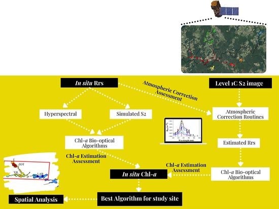
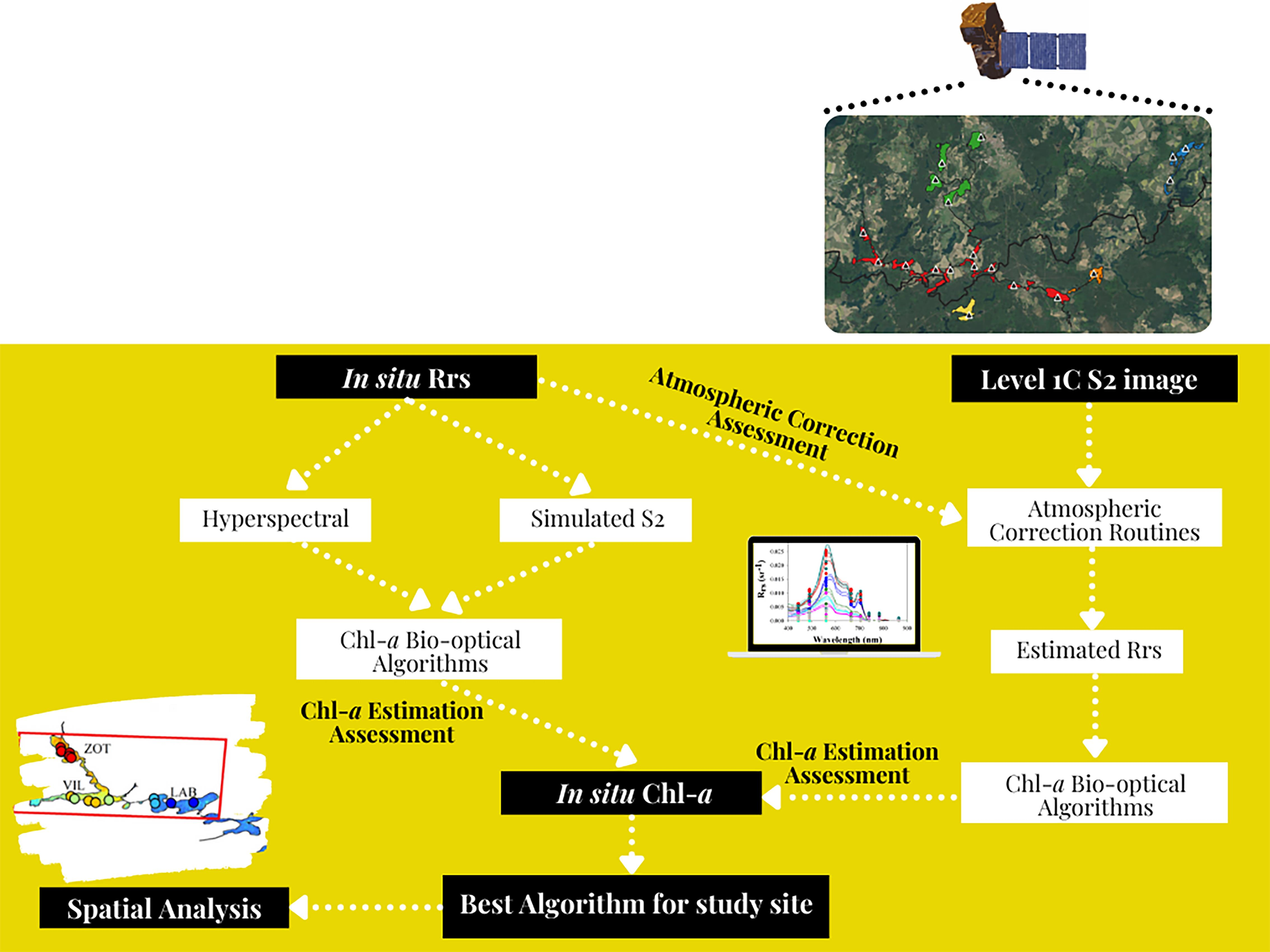
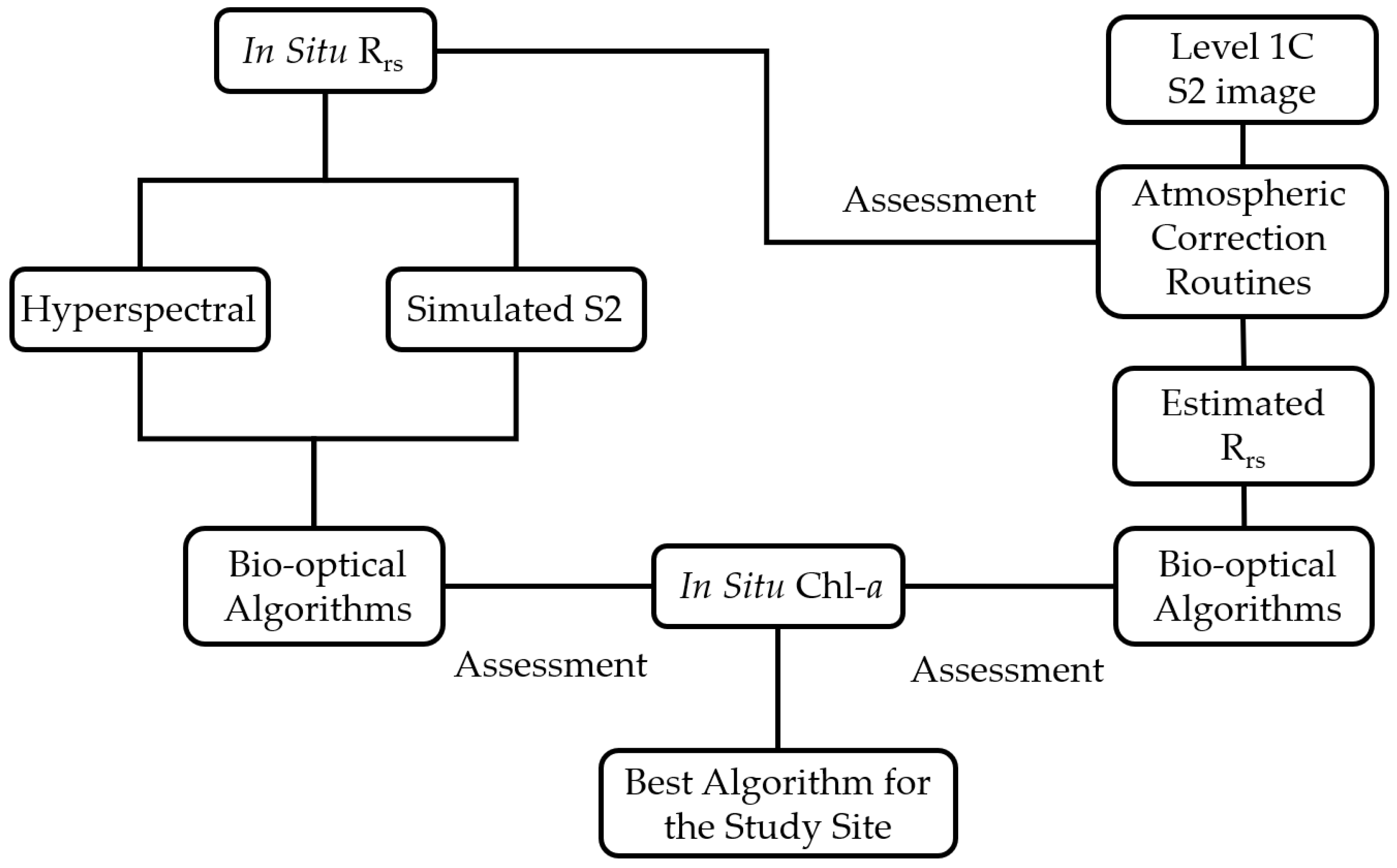
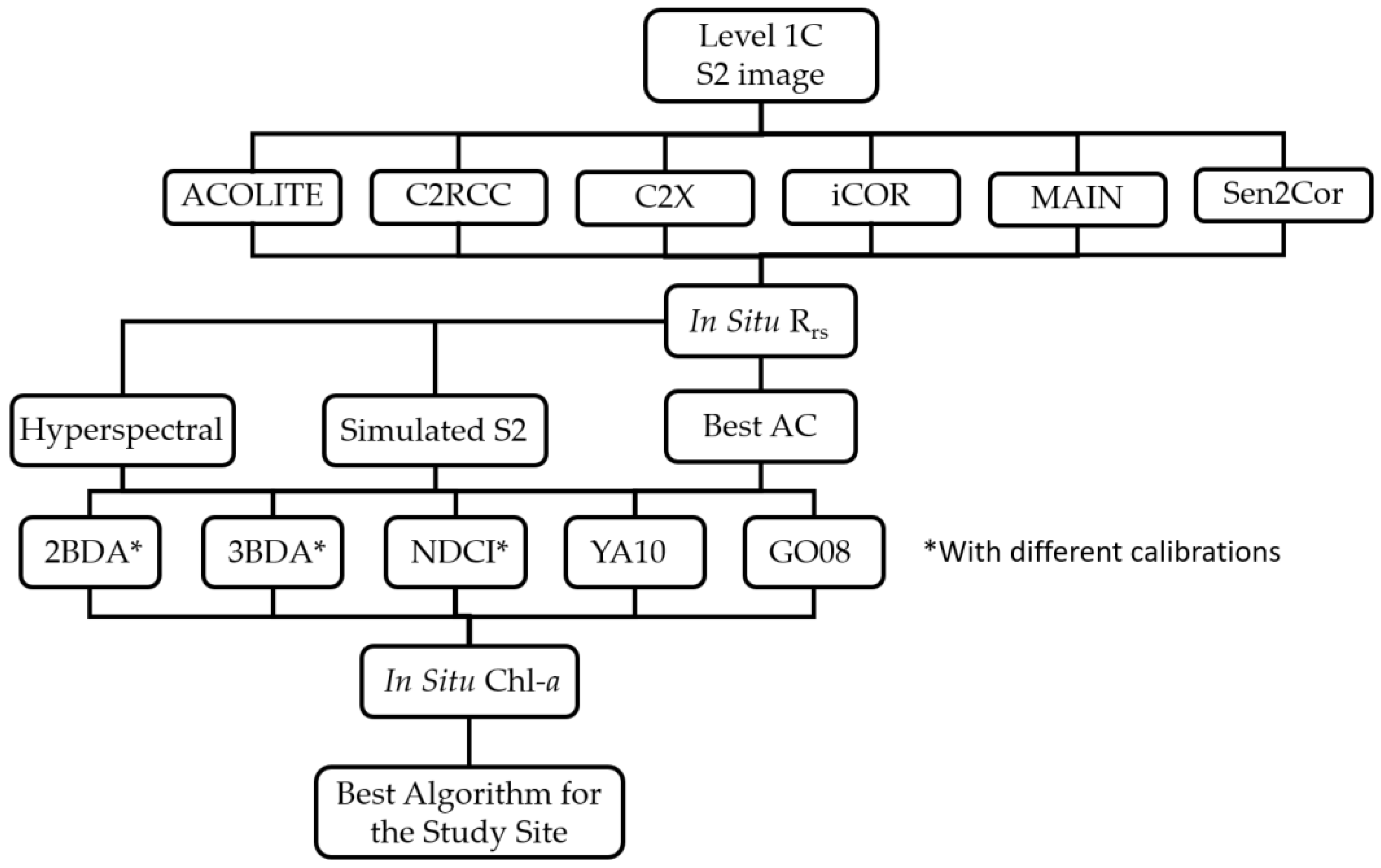
2.4. Image Processing

The following atmospheric correction routines were applied to the Sentinel-2/MSI Level 1 image: (1) ACOLITE [45,46,47], (2) the C2RCC, (3) the Case-2 Extreme Cases (C2X) [48,49,50], (4) image correction for atmospheric effects (iCOR) [51], (5) modified atmospheric correction for inland waters (MAIN) [52] and (6) Sentinel-2 Correction (Sen2Cor) [53]. The Sentinel-2/MSI Level 1 image was first resampled from 20 to 10 m spatial resolution using a scientific image processing toolbox called the Sentinel Application Platform (SNAP v 7.0) developed by Brockmann Consult (Hamburg, Germany), Array Systems Computing (Toronto, Ontario, Canada) and C-S (Paris, France). The selection of these atmospheric corrections was based on the routines that were developed for inland waters (ACOLITE, C2RCC, C2X, iCOR and MAIN) and the standard routine for Sentinel-2 imagery (Sen2Cor). Four of these six atmospheric correction routines were recently evaluated for a Landsat 8/Operational Land Imager (OLI) image over our study site and some showed good performances for the OLI image [34].
ACOLITE is an atmospheric correction routine that uses the dark spectrum fitting approach by default, but can be configured to use the exponential extrapolation approach [45,46,47]. Here, we applied the ACOLITE version Python 20,210,114 routine using the default. C2RCC and C2X rely on a database of radiative transfer simulations of water-leaving radiance and related top-of-atmosphere (TOA) radiances via neural networks. The in-water modeling uses the Hydrolight radiative transfer model (Sequoia, Belevue, WA, USA) and the atmospheric radiative transfer is based on the successive-order-of-scattering (SOS) model [54] with aerosol properties derived from AErosol RObotic NETwork (AERONET) measurements [50]. C2RCC is used for typical ranges of inherent optical properties (IOPs) while C2X is commonly used for extreme ranges of IOPs [48,49,50]. iCOR v 2.0 is an atmospheric correction routine based on MODTRAN 5, requiring information about the solar and viewing angles (Sun Zenith Angle, View Zenith Angle and Relative Azimuth Angle) and a digital elevation model [51]. For the calculation of Rrs, the iCOR product was divided by π. MAIN is an atmospheric correction method implemented on Google Earth Engine by Page et al. [52] and Sen2Cor v. 2.8 is based on scene classification and look-up tables from a radiative transfer model and the surface reflectance was divided by π for an approximate estimation of Rrs [53]. The images were processed according to the default processing parameters and a spatial resolution of 60 m for the comparison among different routines since iCOR and Sen2Cor only process all spectral bands at this resolution.
The best atmospheric correction was used for the extraction of Rrs (single pixel over the sampling location) from the Sentinel-2/MSI image. The extracted Rrs values were used for the computation of chl-a bio-optical algorithms (see Section 2.3) which were compared to the measurements of chl-a concentration (as described in the next Section 2.5).

2.5. Performance Evaluation

To evaluate the performance of the atmospheric correction routines (see Section 2.4) for the Sentinel-2A/MSI image, the Rrs values of each Sentinel-2/MSI spectral band from each pixel corresponding to a ground sample were plotted against the in situ proximal hyperspectral Rrs spectrum (obtained with the spectroradiometers at 1 nm interval). This allowed to evaluate the retrieval of spectral features by the atmospheric correction routines. Additionally, standard statistical metrics were used to evaluate the performance of atmospheric correction routines. Similarly, to evaluate the bio-optical algorithms for the estimation of chl-a concentration (Table 3 and Table 4), standard statistical metrics were used to evaluate their performance using HPLC-based chl-a concentration from water samples.
Brewin et al. [55] and Neil et al. [42] combined error metrics in a quantitative scoring system to rank bio-optical algorithms according to their performance relative to average error statistics. The use of a scoring system was proven to be appropriate for highlighting the algorithms with an underperformance. We assigned scoring points based on the standard deviation distance from 0. For the bias, mean absolute error (MAE), mean square error (MSE) and root mean square error (RMSE), two scoring points were awarded where an algorithm’s error statistics was shown to be within one standard deviation from 0; one scoring point was awarded where an algorithm’s error statistics was between 1 and 2 standard deviations from 0 and no scoring point was awarded where an algorithm’s error statistics was higher than 2 standard deviations from 0. For the coefficient of determination (R2) the same rule for scoring points distribution was applied, however, instead of measuring the distance from zero, we measured the distance from 1. The total number of scoring points was then summed up for each algorithm and the performance rank was allocated based on the total point score. The maximum possible score was 10. Table 4 presents the statistical metrics and rules used to evaluate the performance of each algorithm.
For the evaluation of the bio-optical models the same statistical metrics were calculated for the modeled and measured chl-a concentration.
An overview of the methodological procedure in this study is presented in Figure 2. The in situ data (Rrs and chl-a concentration) are used to ground truth the respective image based estimations. The in situ Rrs (proximal hyperspectral measurements just above the water surface) was also used for the computation of bio-optical algorithms for the estimation of chl-a concentration based on the hyperspectral signal and based on the simulated Sentinel-2 spectral bands. A Level 1C image was used to evaluate different atmospheric correction routines and the best routine was taken for the computation of the bio-optical algorithms used in this comparison. With this comparison we were able to access the best bio-optical algorithm for our study site.

3. Results

Figure 3 presents a detailed overview of the atmospheric correction routines and chl-a bio-optical algorithm assessments. All atmospheric correction routines are listed in Figure 3, however, for the bio-optical algorithms only the algorithms listed in Table 2 are presented. While the 2BDA, the 3BDA and the NDCI were used with several calibrations (Table 3) we did not include the calibrations within Figure 3. Section 3.1 covers the assessment of the atmospheric correction routines while Section 3.2 and Section 3.3 cover the assessment of chl-a bio-optical algorithms.

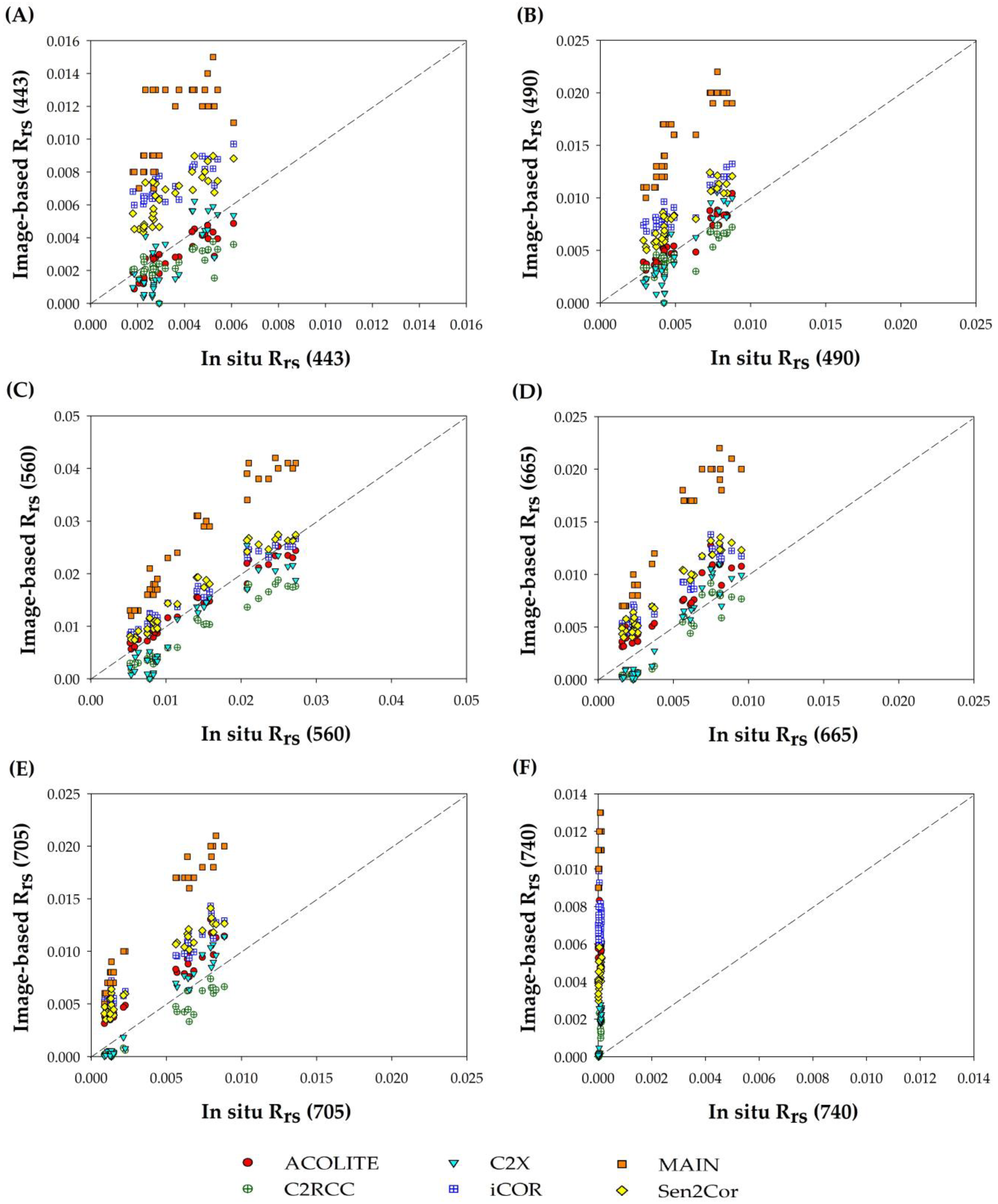
3.1. Atmospheric Correction Routine Comparison

To use the Sentinel-2 image with in situ match-up data, six atmospheric correction routines were applied for the retrieval of Rrs. For the comparison of different atmospheric correction routines, were R2 and RMSE values for the estimation of each spectral band (Table 5). The lowest RMSE (0.001) for band 1 was scored by ACOLITE, C2RCC and C2X. For band 2, the lowest RMSE (0.002) was scored by ACOLITE and C2RCC, while for band 3, only C2RCC scored a RMSE of 0.008. The lowest RMSE for band 4 (0.003) was scored by C2RCC and C2X, while for band 5, only C2RCC scored a RMSE of 0.002. Surprisingly, for band 6, the lowest RMSE (0.002) was scored by C2X and Sen2Cor. iCOR and MAIN did not score the lowest RMSE for any of the spectral bands. Nevertheless, the lowest RMSE did not correspond to the highest R2; for example, there was no correlation between Sen2Cor band 6 (740 nm) and the in situ measured Rrs (R2 = 0); and the RMSE was one of the lowest for this spectral band (RMSE = 0.002).
For a better assessment of the performance of the atmospheric correction routines, scatter plots between the in situ measured Rrs values and the image-estimated Rrs values were evaluated (Figure 4). For band 1(443 nm) and band 2 (490 nm), ACOLITE achieved the best results close to the 1:1 line, followed by the C2X and C2RCC (Figure 4A,B). For band 3, centered at 560 nm (Figure 4C), ACOLITE, iCOR and Sen2Cor achieved good performance; C2X and C2RCC showed a small underestimation of the Rrs and MAIN an overestimation. For band 4 (665 nm), C2X and C2RCC achieved results better than the other atmospheric correction routines being close to the 1:1 line while others were overestimating it (Figure 4D). For the NIR, C2RCC had the best performance followed by C2X, which had some overestimation for the higher values (Figure 4E). Finally, for the band centered at 740 nm, none of the atmospheric correction routines showed a good performance (Figure 4F). Nevertheless, the C2RCC and C2X had the lowest values of Rrs at 740 nm. Considering that most of the algorithms for chl-a retrieval use band 4, band 5 and band 6, C2X was chosen to be the most suitable atmospheric correction routine, especially because it was able to capture the peak around 705 nm for more productive lakes (Figure A1 in the Appendix A).

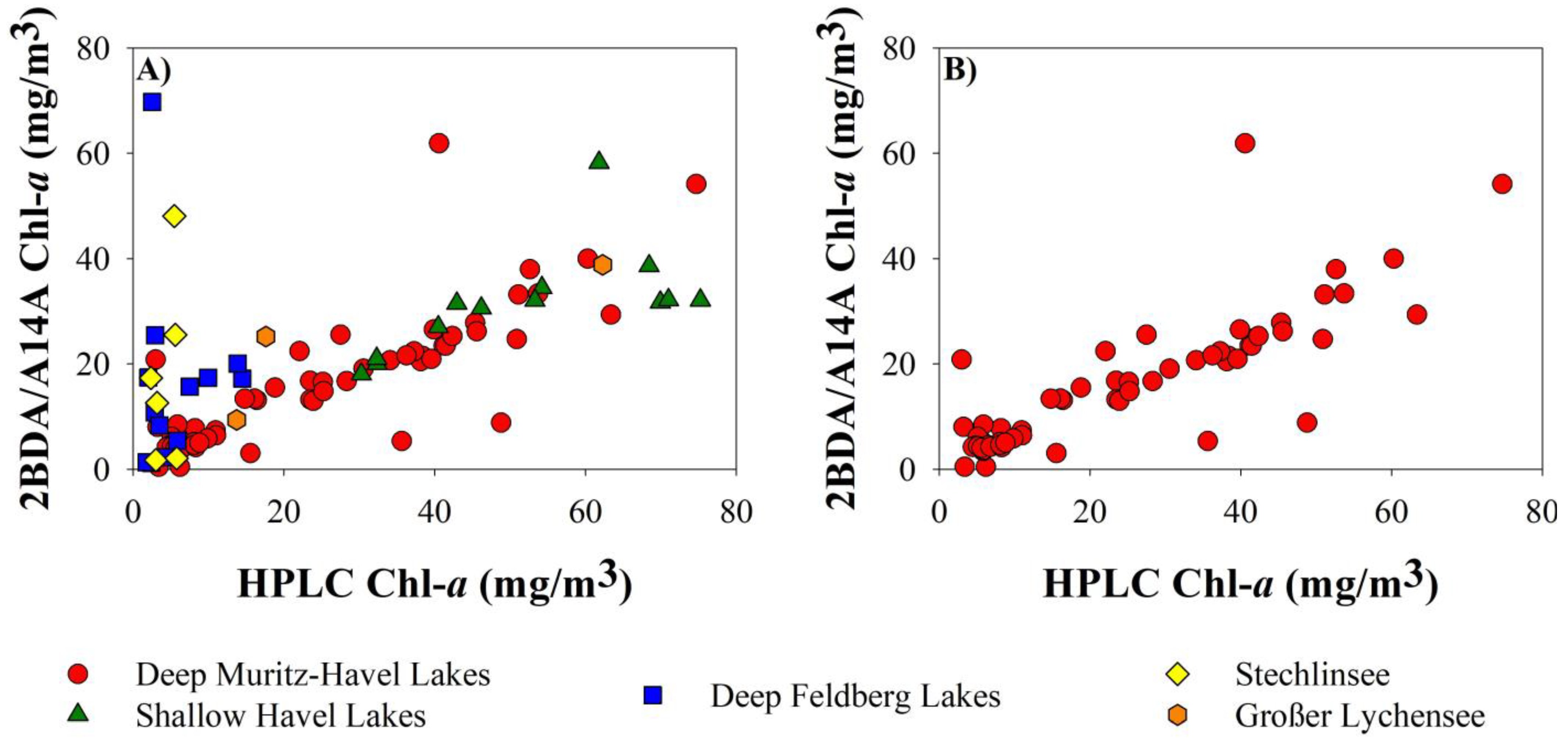
3.2. Comparison of Chl-a Concentration Estimations for the Entire Data Set

The corresponding performance scores for bio-optical algorithms to retrieve chl-a concentration from proximal hyperspectral data for all lakes and locations (n = 97) showed that 2BDA and NDCI were the best-performing algorithms (Figure 5). For the 2BDA, three calibrations obtained a score of 8 points: G11A, A14A and B16A, while for the NDCI, the A14C calibration was the only one to achieve 8 points. Low performances were found for the 3BDA, which got low scores for all calibrations similarly to the YA10 algorithm. For individual statistical metrics (Table A1 in Appendix A), the NDCI using A14C and B16C calibrations achieved the highest R2 value (R2 = 0.479), while 2BDA with B16A calibration achieved the best performance for the bias, MAE, MSE and RMSE (−0.664, 10.196, 287.804 and 16.965, respectively). The chl-a concentration measured via HPLC for the entire data set varied from 1.77 to 75.24 mg/m3 and for this range algorithms based on the red and near infrared bands outperformed other algorithms. However, the overall performance of algorithms was not satisfactory since less than half of the data could be accurately retrieved (Table A1 in Appendix A).
For the simulated Sentinel-2/MSI data set, the performances of chl-a bio-optical algorithms were similar to the hyperspectral data. In addition to the 2BDA and NDCI algorithms, the GO08 (which is based on red and NIR bands) also achieved a score of 8. The main difference between hyperspectral and simulated Sentinel-2/MSI data was the better performance of the simulated data, especially for the 3BDA. This could be related to the use of the 740 nm spectral band in the 3BDA computation, which was used to correct for water absorption. Therefore, the Rrs value of in situ hyperspectral data at this wavelength was low and, since the simulated spectra use a larger band width, the spectral response function of this specific spectral band ended up adding more information. Nevertheless, the statistical estimators (Table A2 in Appendix A) were similar to the lowest RMSE (16.73 mg/m3) being achieved by the 2BDA and A14A combination. Overall, the performance of the simulated Sentinel-2/MSI was similar to the ones using hyperspectral data, where the best algorithm was the 2BDA with the A14A calibration, but the overall performance was still poor.
For the Sentinel-2/MSI image, we obtained 32 matching samples which were collected from one lake group, the Müritz-Havel Lakes (Figure 1 and Section 2.2). The highest scores of 9 points were obtained by the 2BDA using M09A, G11A, A14A, and B16A calibrations and by the 3BDA using the M09B, G11B and B16B calibrations. Statistical metrics (Table A3 in Appendix A) showed that the lowest RMSE was 5.20 mg/m3 estimated via 3BDA using G11B calibration, followed by the 2BDA using A14A (5.70 mg/m3) and G11A (6.50 mg/m3) calibrations. Similarly, to the simulated Sentinel-2/MSI image, the use of satellite imagery seems to improve the performance of the 3BDA algorithm. In the satellite image this overperformance of the 3BDA can be related to the atmospheric correction procedure which overestimates the Rrs value for the 740 nm spectral band (Figure 4). Therefore, the low RMSE is then based on the wrong retrieval of Rrs, which is not appropriate for a universal use of the algorithm. Consequently, the use of the 2BDA with the A14A calibration is more appropriate.

3.3. Comparison of Chl-a Concentration Estimations for the Deep Müritz-Havel Lakes

In Section 3.2, the hyperspectral and simulated Sentinel-2/MSI signals were compared to chl-a concentration measured via HPLC from all 19 lakes, whereas the Sentinel-2/MSI image was compared to data obtained from 6 lakes belonging to the group of Deep Müritz-Havel Lakes with low retention time (or residence time, which is the water age or flushing time, Table 1). To better compare the three approaches, we related the hyperspectral and simulated Sentinel-2/MSI signals to chl-a concentration measured via HPLC from the Deep Müritz-Havel Lakes (n = 68). For the hyperspectral data, the NDCI with the A14C calibration scored 10 points, being the highest among all the algorithms and data sets analyzed (Figure 5 and Figure 6). Overall, the results for the hyperspectral data from the Deep Müritz-Havel Lakes were similar to the previous ones (Figure 5) with 2BDA and NDCI getting the highest scores; however, the lowest RMSE value for the Deep Müritz-Havel lakes was 10.97 mg/m3 (Table A4 in the Appendix A), thereby overestimating chl-a concentrations in comparison to chl-a concentration measured via HPLC ranging from 2.97 to 74.69 mg/m3. For the simulated Sentinel-2/MSI signal for the data from the Deep Müritz-Havel lakes, scores were also similar to the previous analysis of the 19 lakes (Figure 5), however, as for the hyperspectral data the statistical estimators were better for the simulated Sentinel-2/MSI signal, with the lowest RMSE value of 8.94 mg/m3 achieved when using the 2BDA with B16A calibration. Finally, the three data sets from the Deep Müritz-Havel Lakes (hyperspectral, simulated Sentinel-2/MSI signal and Sentinel-2/MSI image) achieved the same scores for the 2BDA using A14A and B16A calibrations, showing that the 2BDA is the only algorithm that is transferable for different sensors.
The comparison between the estimated chl-a concentration by the 2BDA/A14A algorithm and the measured chl-a concentration by the HPLC method is presented for the entire data set (Figure 7A) and for the Deep Müritz-Havel Lakes (Figure 7B). In the entire data set, it was observed that for low chl-a concentration (mainly found at the oligotrophic to mesotrophic waters of Stechlinsee, Breiter Luzin and Schmaler Luzin) was responsible for erroneous estimations from the bio-optical algorithm. This was not observed for the Deep Müritz-Havel Lakes data set (composed mainly of meso- to eutrophic waters). For these lakes, the relationship between estimated and measured chl-a was improved, which might be due to their higher connectivity. The oligotrophic waters from Stechlinsee (yellow rhombus) and Deep Feldberg Lakes (blue squares) are the ones that differ most from the Deep Müritz-Havel Lakes (red circles, Figure 7A). Data from the Deep Müritz-Havel Lakes have chl-a concentrations varying from 2.97 to 74.69 mg/m3; therefore, having different trophic states—oligotrophic, mesotrophic and eutrophic (Figure 7B). The retrieval of chl-a from remote sensing data was improved for the Deep Müritz-Havel Lakes data set, even when different trophic states were included. This unexpected result shows that while trophic state is important for the characterization of optical water types [42], other variables could contribute for the improvement of the performance of bio-optical algorithms. In this case, besides the difference in the retention time from the Deep Müritz-Havel Lakes to the Stechlinsee and Deep Feldberg Lakes (Table 1), the land use in the catchment area is also different, with a stronger agriculture presence in the Deep Müritz-Havel Lakes, and a forest coverage for Stechlinsee and Deep Feldberg Lakes.

4. Discussion

4.1. Performance of Algorithms

Recently, Warren et al. [56] evaluated six atmospheric correction routines for Sentinel-2/MSI images over inland waters. In their analysis, C2RCC achieved good performance for inland waters, achieving the lowest root-mean-square deviation (RMSD). Ogashawara et al. [34] evaluated the use of ACOLITE, iCOR, C2RCC and C2X atmospheric correction routines for the Landsat 8/OLI images and noticed that ACOLITE was good for the visible range, while C2RCC and C2X performed better in the red to near-infrared spectral bands. Overall, the results presented in Section 3.1 of this study corroborates with previous studies on atmospheric corrections over inland waters. Additionally, the atmospheric correction procedure showed to be an important factor for the performance of bio-optical algorithms, especially on the algorithms that use the spectral band centered at 740 nm which is usually sign of an uncorrected adjacency effect [57]. To avoid these effects from adjacent pixels, the use of a tighter subset of the aquatic system can improve the performance of the atmospheric correction routine.
There is a strong relationship (R2 of 0.96) between the image and the simulated spectra for bands 4 and 5, but a poor relationship (R2 of 0.28) exists for band 6 (centered at 740 nm) (Figure 8). This emphasizes that the overperformance of some bio-optical algorithms on the Sentinel-2/MSI image is caused by the overestimation of Rrs at 740 nm (Figure 4). This poor performance of the atmospheric correction routine for the spectral band centered at 740 nm has been observed by Warren et al. [56] who noticed the same problem for different atmospheric correction routines for inland waters. Therefore, atmospheric correction routines need to improve the retrieval of the spectral information in the near-infrared, especially for inland waters. This highlights the need for an atmospheric correction evaluation before the use of any satellite imagery for bio-optical modeling studies.
It is important to note that the results on the evaluation of the atmospheric correction in this study are solely based on a single image. More images are needed for a complete evaluation of the atmospheric correction routines for Sentinel-2/MSI images under different atmospheric conditions. Yet, to correctly use the image over our study area, we assessed the best atmospheric correction for this single scene for the most appropriate application of chl-a bio-optical algorithms.
The results presented in Section 3.2 and Section 3.3 showed that for chl-a retrieval, bio-optical algorithms using the combination of red and near-infrared spectral bands achieved the best performances. This finding agrees with Gurlin et al. [39], who also used proximal hyperspectral data collected at 20 sand pit lakes in Nebraska in two different seasons. For these lakes, the simple 2BDA algorithm was able to outperform complex algorithms, suggesting the need to return and use the simple two-band NIR-red model. This suggestion was also supported by a later publication by Augusto-Silva et al. [40] who used proximal hyperspectral data from 40 sampling points in a tropic hydroelectric reservoir in Brazil to evaluate various bio-optical algorithms for chl-a estimation in different seasons. For these mesotrophic waters, the 2BDA algorithm out-competed other bio-optical algorithms when using proximal hyperspectral data. Beck et al. [41] showed that both 2BDA and NDCI had good performances for a synthetic Sentinel-2/MSI image derived from a hyperspectral airborne image. Neil et al. [42] compiled a big data set containing 2807 proximal hyperspectral data sets from 185 aquatic systems worldwide. In this large and unique data set, the authors compared 48 combinations of bio-algorithms using different calibrations and ended up with three bio-optical algorithms which should be used for (1) oligotrophic waters, (2) meso-to-eutrophic waters and (3) for hypereutrophic waters. For the meso-to-eutrophic waters, authors suggested the use of the 2BDA algorithm with G11A calibration which was similar to the findings in this study; however, here, A14A calibration was the best, and this was not evaluated by the authors. Additionally, Neil et al. [42] also suggested that 2BDA should be the algorithm to be used when there is no information about the trophic state of the lake. The performance of 2BDA was also supported by Soomets et al. [58], who showed that 2BDA had the best performance for the entire data set from different Estonian and Latvian lakes. All these studies and the results presented in Section 3.2 and Section 3.3 suggest that the use of formulations, which provide a unitless product like the 2BDA and NDCI algorithms, reduce the uncertainties in the estimation of chl-a concentration by excluding the seasonal solar azimuth differences and atmospheric contributions.

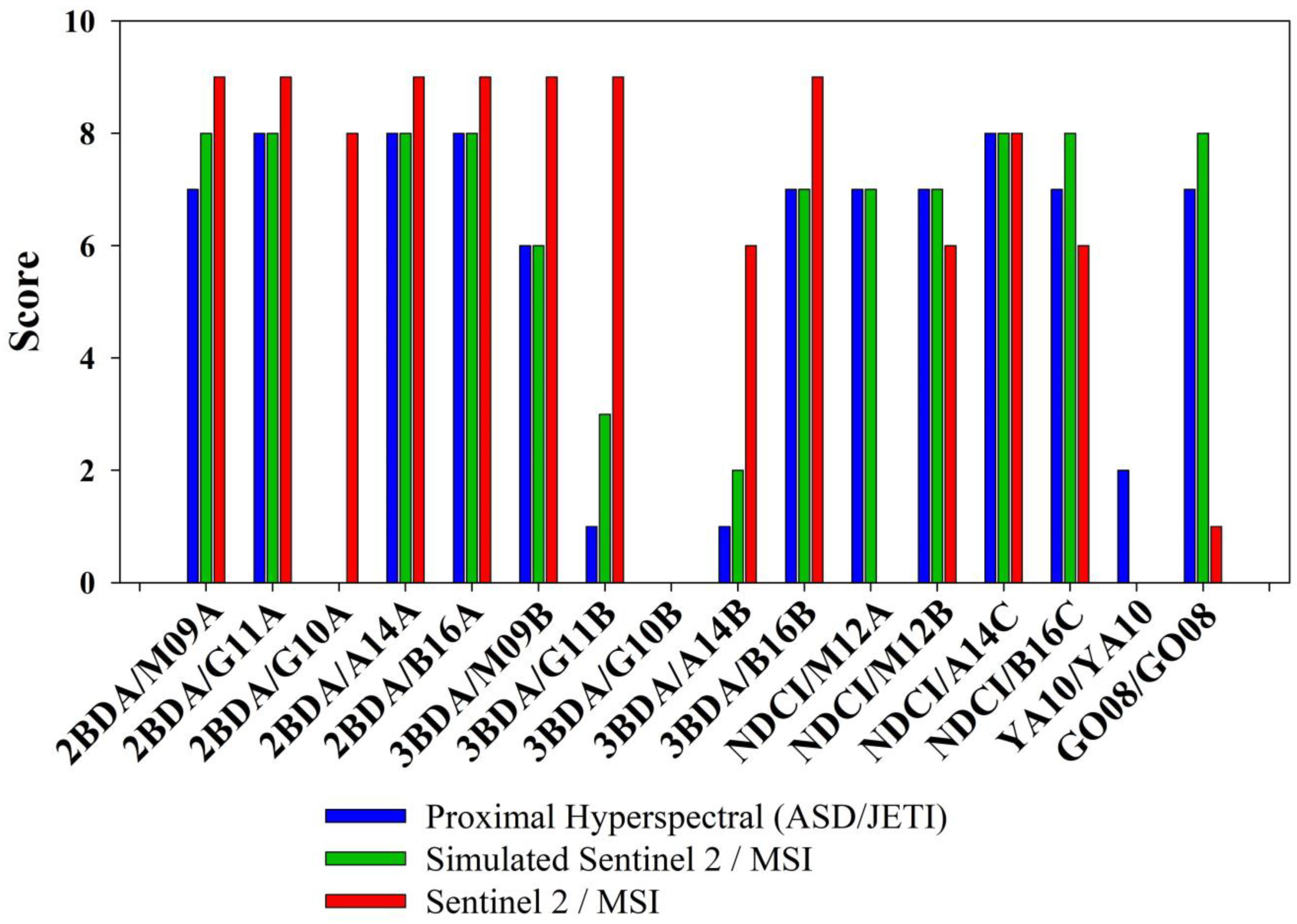
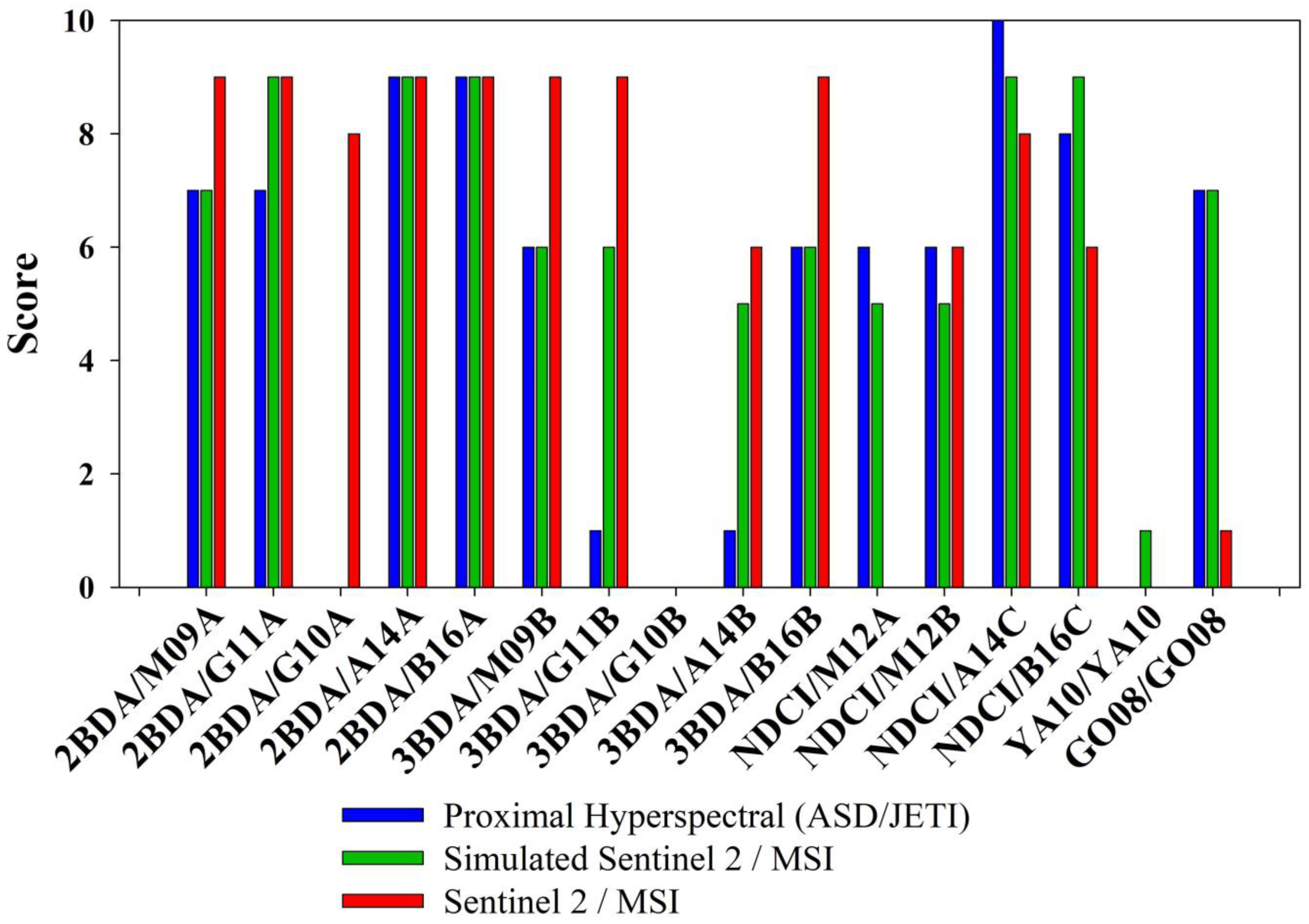
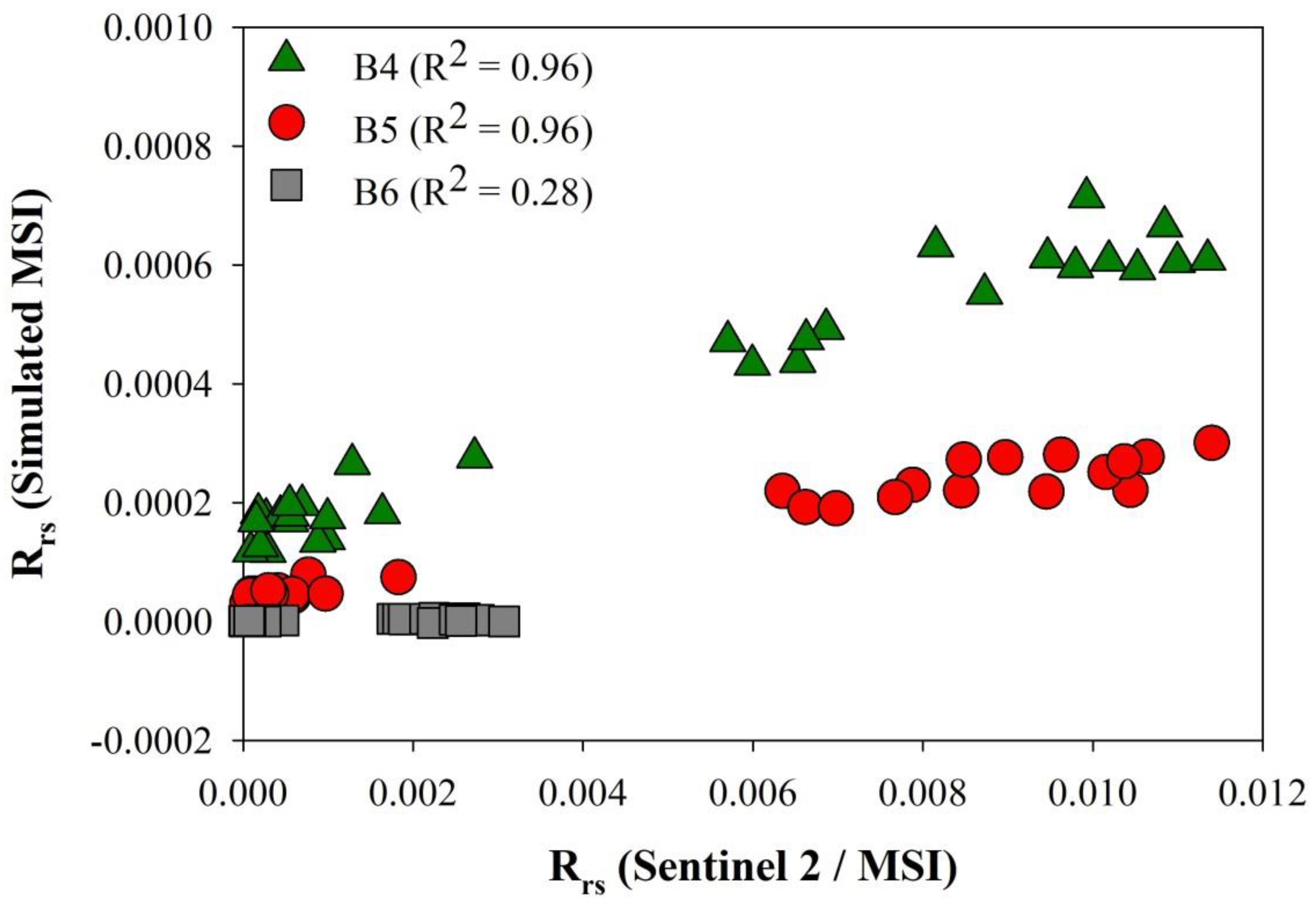
4.2. Bio-Optical Algorithms Transferability to Different Sensors

For the estimation of chl-a concentrations, the three best combinations of bio-optical algorithms and calibrations for hyperspectral data, based on the scores (Figure 5) and statistical metrics (Table A1 in the Appendix A) for all 19 lakes were: (1) 2BDA/B16A; (2) 2BDA/A14A; and (3) NDCI/A16C, respectively. For the simulated Sentinel-2/MSI signal (Table A2 in the Appendix A), the three best algorithms and calibrations were: (1) 2BDA/A14A, (2) 2BDA/B16A; and (3) NDCI/A16C, respectively. Consideration of all lakes sampled (Figure 1) indicates that the 2BDA represents the algorithm that is most consistent for the estimation of chl-a concentration.
When considering only the Deep Müritz-Havel lakes (meso- to eutrophic waters), the best three algorithms were the same for the hyperspectral data (Table 6 and Table A4 in the Appendix A) and for the simulated Sentinel-2/MSI signal (Table A5 in the Appendix A): (1) 2BDA/B16A, (2) 2BDA/A14A and (3) NDCI/A16C, respectively. For the Sentinel-2/MSI image, the best bio-optical algorithms for chl-a concentration were: (1) 3BDA/G11B, (2) 2BDA/A14A and (3) 2BDA/G11A. However, since the 3BDA uses band 6, which was clearly affected by the atmospheric correction, the performance of this algorithm is biased. Thus, considering these three data sets, 2BDA/A14A was the only tested bio-optical algorithm that can be used for all data sets with a good performance, since 2BDA/B16A did not perform well for the Sentinel-2/MSI image.
While most studies comparing bio-optical algorithms evaluate their accuracy based on estimation errors of water quality parameters [39,40,41,42], in this study, not only error metrics were used for quality assessment of each bio-optical algorithm. We also added a new perspective for algorithm evaluation, i.e., its capability to be transferred to different sensors. Thus, we suggest that for a high versatility, a bio-optical algorithm should not only be accurate but also transferable to other sensors, and the combination of both should be routinely considered in future performance evaluations.

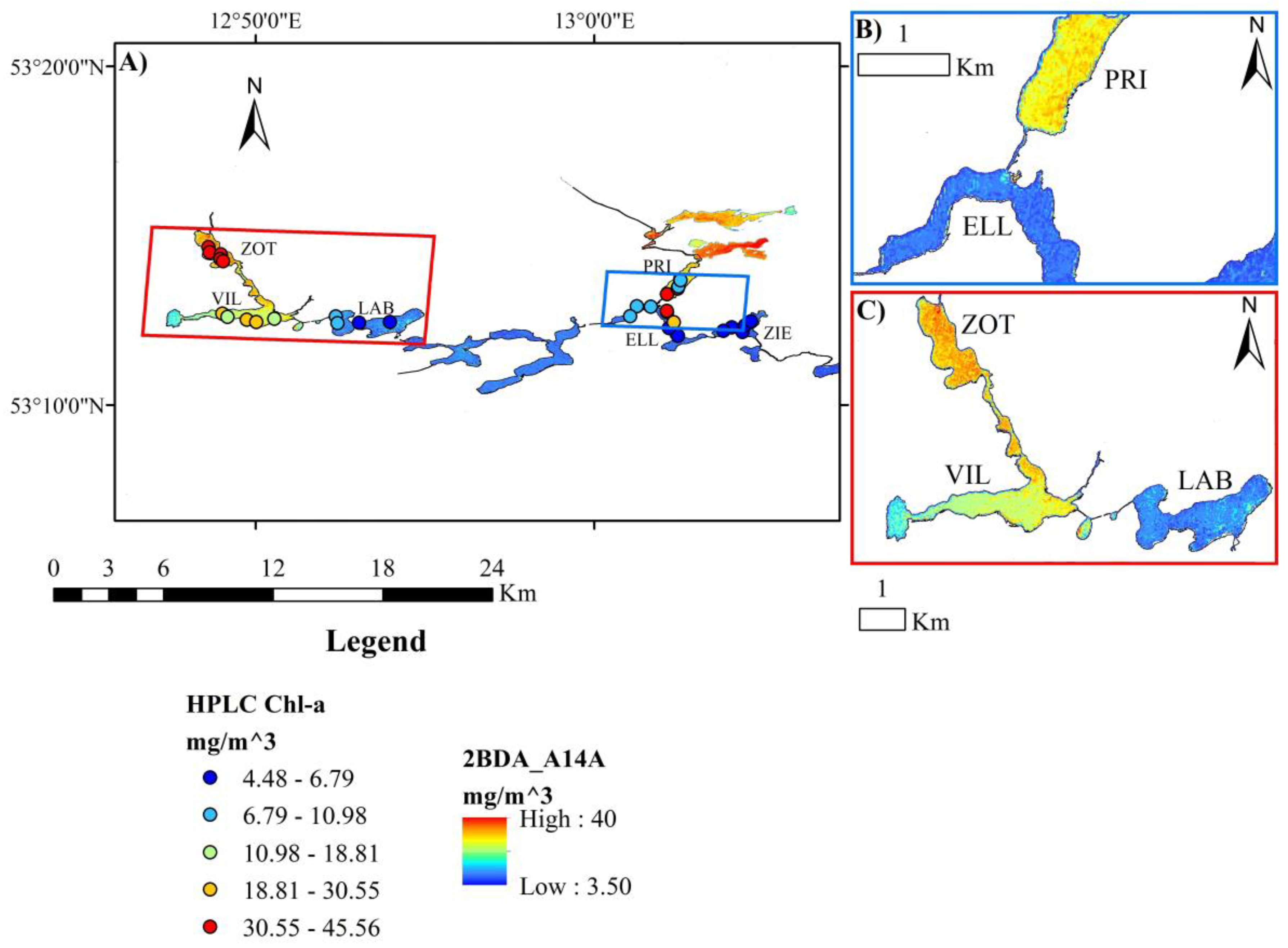
4.3. Chl-a Retrieval from the Sentinel-2/MSI Image and Spatial Patterns

2BDA/A14A was applied to the Sentinel-2/MSI image for the pixels, which exclusively contain water (Figure 9). The final product provides the spatial distribution of chl-a concentration for some of the Müritz-Havel Lakes, including the six lakes for which we have collected both in situ water samples for chl-a measurements and hyperspectral data. A gradient of chl-a concentration can be observed from ZOT over VIL to LAB (Figure 9C) where concentrations were highest in ZOT and decreased toward LAB along the flow direction of the Müritz-Havel river system. Additionally, VIL showed a gradient within the lake, with low chl-a concentrations in the western part of the lake, where it connects to the oligotrophic Schwarzer See and high chl-a concentrations in the northern area, where it connects to ZOT. Another heterogeneous spatial pattern was observed among ELL, PRI and ZIE (Figure 9B), where ELL and ZIE along the Upper Havel river system showed low chl-a concentrations, while PRI showed significantly higher chl-a concentrations. In the region where ELL is connected to PRI (Figure 9B), we observed increased chl-a concentration indicating that chl-a-rich water from PRI was entering into the less chl-a-rich ELL.
Our results (Figure 6 and Figure 8, Table A1, Table A2, Table A3, Table A4 and Table A5 in the Appendix A) demonstrate that remote sensing measurements can retrieve chl-a with low errors in lakes. Based on the in situ HPLC measurements of chl-a, the selected bio-optical algorithm was applied to the satellite imagery and was able to retrieve chl-a concentrations with a bias as low as −0.03 mg/m3 (see Table 4 for the details on statistical metrics). The retrieved chl-a concentrations were consistent with the trophy of the studied lakes as indicated by the trophic index from LAWA (Table 1) which shows that ZOT, VIL and PRI have higher index values than LAB, ELL and ZIE.
Our study of river-connected lakes adds new insights on how remote sensing data, obtained with medium resolution spaceborne sensors, can be used to successfully monitor water quality parameters and to acquire spatial patterns between and within lakes. To better understand the environmental dynamics of lake systems the information about the spatial heterogeneity within and between lakes can, for example, be used to improve water sampling strategies by selecting representative areas and appropriate timing for in situ sampling. While the use of satellite data cannot replace in situ monitoring programs, the use of remote sensing data for lake monitoring would rather complement traditional data by providing a new dimension of spatial and temporal data acquisition and resolution [59]. Although the use of remote sensing data is limited by cloud cover, with MSI being present on both Sentinel-2A and Sentinel-2B, the temporal resolution is duplicated and could, in principle, acquire 100 images per year in our study area. Even if cloud cover affects half of the images, the use of satellite data could still increase the number of observations by a factor of 4 in comparison to traditional monitoring programs that typically collect data monthly or mostly less frequently. Additionally, the spatial distribution of chl-a can assist the planning of field campaigns and implementation of early warning systems for algal bloom developments. Future constellations of nanosatellites equipped with Earth Observation sensors capable of monitoring in water chl-a can improve the temporal acquisition of images and become important tools to complement novel lake management strategies.

5. Conclusions

We evaluated several algorithms for the estimation of chl-a concentration in river-connected lakes using hyperspectral, simulated Sentinel-2/MSI signal and a single Sentinel-2/MSI image. We used chl-a concentrations measured via HPLC from 19 lakes in North-East Germany collected from June to October 2019. Unfortunately, due to cloud cover, only one Sentinel-2/MSI image acquired on 26 July 2019 matched up with in situ radiometric and chl-a concentration data. Therefore, the evaluation of the atmospheric correction routines is limited to only one atmospheric condition. For the estimation of chl-a concentrations, red and near infrared algorithms such as 2BDA and NDCI were the best performing algorithms for the hyperspectral and simulated Sentinel-2/MSI signals (Figure 5 and Figure 6, Table A1 and Table A2, Table A4 and Table A5). For the satellite image, although the 3BDA showed the best performance (Figure 5 and Figure 6 and Table A3), this result is erroneous since it uses a spectral band which showed poor performance of the atmospheric correction procedure (Figure 4 and Figure 8). Therefore, the best performing algorithm for the Sentinel-2/MSI image was the 2BDA which showed solid performance when applied to different sensors and data sets. While there are several studies using in situ hyperspectral Rrs data to simulate Sentinel-2 spectral bands, we highlight here the need of more studies using satellite images for calibration of algorithms. Thus, another limitation of this study was the use of calibrations which were derived from hyperspectral data instead of the Sentinel-2 images.
For the atmospheric correction of the Sentinel-2/MSI image, we evaluated the use of ACOLITE, C2RCC, C2X, iCOR, MAIN and Sen2Cor routines and compared them to in situ hyperspectral Rrs data. Based on statistical metrics, scatterplots (Figure 4) and the retrieval of the spectral shape (Figure A1) we selected C2X as the best performing atmospheric correction routine for our study site. The C2X routine was able to retrieve similar spectral shapes and the magnitude of in-situ Rrs spectra, especially for bands 4, 5 and 6 which are commonly used for chl-a algorithms. However, due to the limited match ups with satellite imagery, future studies should focus on a comparison of atmospheric correction routines under different atmospheric conditions (not only in a clear sky day) for aquatic systems with different trophic states and located in different latitudes. Additionally, based on the underperformance from all atmospheric correction routines for band 6 (740 nm) future studies should focus on the improvement of the retrieval of Rrs in the near-infrared–which is usually affected by adjacency effects.
Finally, the spatial assessment of the results unraveled high spatial heterogeneity in chl-a concentrations within lakes and gradients along a chain of river-connected lakes. These spatial heterogeneities indicate effects of connectivity among a cascade of lakes or interconnected lakes in a lake-river system, which can be explained by a gradient in biogeochemical variability and highlight the influence of a neighboring lake of higher or lower trophic state. These observations are important not only to understand the environmental dynamics of river-connected lakes, but also for the management of inland water systems. Thus, the remote sensing technology has the potential to complement and streamline existing monitoring programs by increasing temporal and spatial resolution for pattern detection to help understanding the dynamics of highly abundant small-sized aquatic systems.

Author Contributions

Conceptualization, I.O., C.K., K.K., A.J., H.-P.G., T.R., F.H., J.C.N., S.A.B. and S.W.; methodology, I.O., A.J., C.K., K.K., S.A.B. and S.W.; software, I.O.; validation, I.O., C.K., A.J., S.A.B. and S.W.; formal analysis, I.O. and C.K.; investigation, I.O. and C.K.; resources, S.A.B., S.W., J.C.N., H.-P.G., T.R. and F.H.; data curation, I.O. and C.K.; writing—original draft preparation, I.O.; writing—review and editing, I.O., C.K., A.J., K.K., T.R., H.-P.G., F.H., J.C.N., S.W. and S.A.B.; visualization, I.O.; supervision, S.A.B., S.W., H.-P.G. and J.C.N.; project administration, S.A.B. and S.W.; funding acquisition, S.A.B., J.C.N., A.J., H.-P.G., F.H. and S.W. All authors have read and agreed to the published version of the manuscript.

Funding

This work was funded by a collaborative research grant of the Leibniz Competition within the project CONNECT–Connectivity and synchronization of lake ecosystems in space and time (No. K45/2017).

Institutional Review Board Statement

Not applicable.

Informed Consent Statement

Not applicable.

Data Availability Statement

The data presented in this study are available on request from the corresponding author. The data are not publicly available because the CONNECT project is still on going and results are still being processed.

Acknowledgments

We thank Liu Liu, Carolin Berndt, Elena Ziemann, Kai Thielen, Michael Sachtleben, Matthias Bodenlos, Günter Schreck and Lena Mellin for technical and sampling support, as well as Marén Lentz, Monika Degebrodt, Monika Papke, Solvig Pinnow, Uta Mallok, Elke Mach and Elfi Huth for support on laboratorial analysis. We also thank Gabriel Singer for helpful comments during the writing of the manuscript. We also thank Eckhard Kohlhas and Ilona Korczynski from the Ministry of Agriculture and the Environment Mecklenburg-Vorpommern for providing morphometric data and trophic index values of the sampled lakes. We thank Martin Bork, the team from the Seenfischerei “Obere Havel”, and the Seenfischerei “Uckermark-Fisch” for support (boat storage and access to the lakes).

Conflicts of Interest

The authors declare no conflict of interest.

Appendix A

In this appendix we present the statistical metrics used for chl-a estimations from hyperspectral data (Table A1) and simulated Sentinel-2/MSI signal (Table A2) for all lakes; statistical metrics for Sentinel-2/MSI image (Table A3) for six of the Havel-Müritz Lakes, as well as the statistical metrics used for chl-a estimations from hyperspectral data (Table A4) and simulated Sentinel-2/MSI signal (Table A5) for the Havel Lakes.
Table A1. Statistical metrics (R2, bias, MAE, MSE, RMSE) for different chl-a bio-optical algorithms from proximal hyperspectral in situ data from all lakes. 2BDA with G10A calibration and 3BDA with G10B calibration did not produce results. Shaded cells indicate the best values of each metric.
Statistical Metric2BDA/
M09A
2BDA/
G11A
2BDA/
A14A
2BDA/
B16A
3BDA/
M09B
3BDA/
G11B
3BDA/
A14B
3BDA/
B16B
NDCI/
M12A
NDCI/
M12B
NDCI/
A14C
NDCI/
B16C
YA10/
YA10
GO08/
GO08
R20.420.320.420.420.0010.0070.0010.0010.140.150.480.480.470.44
bias13.218.556.04−0.66−6.75−27.70−21.47−13.4410.9711.388.6510.2743.8814.17
MAE18.5916.1412.4010.1929.3444.2455.5223.3917.3317.4213.4318.0063.5417.86
MSE485.53483.76293.55287.803742.7128,720.8021,043.931227.24505.51516.01321.31508.128655.17451.39
RMSE22.0321.9917.1316.9661.18169.47145.0635.0322.4822.7117.9222.5493.0321.24
Table A2. Statistical metrics (R2, bias, MAE, MSE, RMSE) for different chl-a bio-optical algorithms from simulate Sentinel−2/MSI spectral bands from proximal hyperspectral in situ data from all lakes. 2BDA with G10A calibration and 3BDA with G10B calibration did not produce results. Shaded cells indicate the best values of each metric.
Statistical Metric2BDA/
M09A
2BDA/
G11A
2BDA/
A14A
2BDA/
B16A
3BDA/
M09B
3BDA/
G11B
3BDA/
A14B
3BDA/
B16B
NDCI/
M12A
NDCI/
M12B
NDCI/
A14C
NDCI/
B16C
YA10/
YA10
GO08/
GO08
R20.400.320.400.400.0020.010.0020.0020.240.250.460.460.380.43
bias10.166.423.96−3.46−1.75−14.51−8.97−11.3111.7612.196.494.6548.8111.93
MAE15.5613.8711.7310.8822.9730.4836.2321.4716.1016.2712.6913.1472.2415.60
MSE392.05403.57279.96287.202304.7812,981.3611,894.81924.42474.60482.69310.44335.8411,712.69394.83
RMSE19.8020.0916.7316.9548.01113.93109.0630.4021.7821.9717.6218.33108.2219.87
Table A3. Statistical metrics (R2, bias, MAE, MSE, RMSE) for different chl-a bio-optical algorithms from Sentinel-2 / MSI image for Müritz-Havel Lakes. 3BDA with G10B calibration and GO08 with GO08 calibration did not produce results. Shaded cells indicate the best values of each metric.
Statistical Metric2BDA/
M09A
2BDA/
G11A
2BDA/
G10A
2BDA/
A14A
2BDA/
B16A
3BDA/
M09B
3BDA/
G11B
3BDA/
A14B
3BDA/
B16B
NDCI/
M12A
NDCI/
M12B
NDCI/
A14C
NDCI/
B16C
YA10/
YA10
GO08/
GO08
R20.930.94 0.930.930.930.940.930.930.720.850.900.900.870.94
bias−7.60−4.60−4.97−0.03−3.85−7.29−2.03−26.008.531847.1417.9115.12−30.48−75.29452.97
MAE7.824.915.203.546.557.513.1326.918.981848.3328.3121.0830.4883.77460.71
MSE91.6642.6356.0632.6265.7385.5227.051118.88108.746,214,128.101205.85645.091605.9611,403.78899,341.67
RMSE9.576.537.495.718.119.255.2033.4510.432492.8234.7325.4040.07106.79948.34
Table A4. Statistical metrics (R2, bias, MAE, MSE, RMSE) for different chl-a bio-optical algorithms from proximal hyperspectral in situ data from Müritz-Havel Lakes. 2BDA with G10A calibration and 3BDA with G10B calibration did not produce results. Shaded cells indicate the best values of each metric.
Statistical Metric2BDA/
M09A
2BDA/
G11A
2BDA/
A14A
2BDA/
B16A
3BDA/
M09B
3BDA/
G11B
3BDA/
A14B
3BDA/
B16B
NDCI/
M12A
NDCI/
M12B
NDCI/
A14C
NDCI/
B16C
YA10/
YA10
GO08/
GO08
R20.690.590.690.690.0000.0010.0000.0000.200.210.710.710.660.68
bias17.4512.868.983.12−4.01−14.74−15.02−12.2412.7913.3410.9215.6644.4517.54
MAE18.9615.2910.557.0425.0831.0544.2221.0416.6416.8411.7517.8553.9318.39
MSE423.47328.85193.48120.251777.255899.489552.48741.46435.94447.71247.49456.335306.31419.30
RMSE20.5818.1313.9110.9742.1676.8197.7427.2320.8821.1615.7321.3672.8420.48
Table A5. Statistical metrics (R2, bias, MAE, MSE, RMSE) for different chl-a bio-optical algorithms from simulate Sentinel-2 / MSI spectral bands from proximal hyperspectral in situ data from Müritz-Havel Lakes. 2BDA with G10A calibration and 3BDA with G10B calibration did not produce results. Shaded cells indicate the best values of each metric.
Statistical Metric2BDA/
M09A
2BDA/
G11A
2BDA/
A14A
2BDA/
B16A
3BDA/
M09B
3BDA/
G11B
3BDA/
A14B
3BDA/
B16B
NDCI/
M12A
NDCI/
M12B
NDCI/
A14C
NDCI/
B16C
YA10/
YA10
GO08/
GO08
R20.630.560.630.630.030.020.030.030.400.410.650.650.510.62
bias8.546.344.00−0.191.36−0.980.28−5.988.598.955.155.4630.039.23
MAE9.517.805.934.8811.4111.1413.8111.849.569.776.637.1940.559.75
MSE198.43163.51113.3779.84411.49341.631200.57321.15255.03261.26144.96149.025304.52222.90
RMSE14.0912.7910.658.9320.2818.4834.6517.9215.9716.1612.0412.2172.8314.93
Figure A1. Comparison between Rrs spectral from proximal hyperspectral data (solid lines) and the best atmospheric correction routines for Sentinel-2/MSI (points). (A) ACOLITE, (B) C2RCC, (C) C2X.
Remotesensing 13 01542 g0a1

References

  1. Cole, J.J.; Praire, Y.T.; Caraco, N.F.; McDowell, W.H.; Tranvik, L.J.; Striegl, R.G.; Duarte, C.M.; Kortelainen, P.; Downing, J.A.; Middelburg, J.J.; et al. Plumbing the Global Carbon Cycle: Integrating Inland Waters into the Terrestrial Carbon Budget. Ecosystems 2007, 10, 171–184. [Google Scholar] [CrossRef] [Green Version]
  2. Williamson, C.E.; Dodds, W.; Kratz, T.K.; Palmer, M.A. Lakes and streams as sentinels of environmental change in terrestrial and atmospheric processes. Front. Ecol. Environ. 2008, 6, 247–254. [Google Scholar] [CrossRef]
  3. Tundisi, J.G.; Matsumura-Tundisi, T.; Tundisi, J.E.M. Reservoirs and human well being: New challenges for evaluating impacts and benefits in the neotropics. Braz. J. Biol. 2008, 68, 1133–1135. [Google Scholar] [CrossRef]
  4. Häder, D.-P.; Banaszak, A.T.; Villafañe, V.E.; Narvarte, M.A.; González, R.A.; Helbling, E.W. Anthropogenic pollution of aquatic ecosystems: Emerging problems with global implications. Sci. Total Environ. 2020, 713, 136586. [Google Scholar] [CrossRef]
  5. Wurtsbaugh, W.A.; Paerl, H.W.; Dodds, W.K. Nutrients, eutrophication and harmful algal blooms along the freshwater to marine continuum. Wiley Interdiscip. Rev. Water 2019, 6, e1373. [Google Scholar] [CrossRef]
  6. UNEP International Environmental Technology Centre. Planning and Management of Lakes and Reservoirs: An Integrated Approach to Eutrophication, 1st ed.; UNEP International Environmental Technology Centre: Shiga, Japan, 1999. [Google Scholar]
  7. Reinart, A.; Kutser, T. Comparison of different satellite sensors in detecting cyanobacterial bloom events in the Baltic Sea. Remote Sens. Environ. 2006, 102, 74–85. [Google Scholar] [CrossRef]
  8. Moses, W.J.; Gitelson, A.A.; Berdnikov, S.; Povazhnyy, V. Estimation of chlorophyll-a concentration in case II waters using MODIS and MERIS data—Successes and challenges. Environ. Res. Lett. 2009, 4, 1–8. [Google Scholar] [CrossRef] [Green Version]
  9. Duan, H.; Ma, R.; Xu, J.; Zhang, Y.; Zhang, B. Comparison of different semi-empirical algorithms to estimate chlorophyll-a concentration in inland lake water. Environ. Monit. Assess. 2010, 170, 231–244. [Google Scholar] [CrossRef] [PubMed]
  10. Stech, J.L.; Lima, I.B.T.; Novo, E.M.L.M.; Silva, C.M.; Assireu, A.T.; Lorenzzetti, J.A. Telemetric monitoring system for meteorological and limnological data acquisition. Int. Ver. Theor. Angew. Limnol. 2006, 29, 747–1750. [Google Scholar] [CrossRef]
  11. Marcé, R.; George, G.; Buscarinu, P.; Deidda, M.; Dunalska, J.; de Eyto, E.; Flaim, G.; Grossart, H.-P.; Istvanovics, V.; Lenhardt, M.; et al. Automatic High Frequency Monitoring for Improved Lake and Reservoir Management. Environ. Sci. Technol. 2016, 50, 10780–10794. [Google Scholar] [CrossRef]
  12. Gons, H.J.; Auer, M.T.; Effler, S.W. MERIS satellite chlorophyll mapping of oligotrophic and eutrophic waters in the Laurentian Great Lakes. Remote Sens. Environ. 2008, 112, 4098–4106. [Google Scholar] [CrossRef]
  13. Dall’Olmo, G.; Gitelson, A.A. Effect of bio-optical parameter variability on the remote estimation of chlorophyll-a concentration in turbid productive waters: Experimental results. Appl. Opt. 2005, 44, 412–422. [Google Scholar] [CrossRef] [Green Version]
  14. Mishra, S.; Mishra, D.R. Normalized difference chlorophyll index: A novel model for remote estimation of chlorophyll-a concentration in turbid productive waters. Remote Sens. Environ. 2012, 117, 394–406. [Google Scholar] [CrossRef]
  15. Olmanson, L.G.; Bauer, M.E.; Brezonik, P.L. A 20-year Landsat water clarity census of Minnesota’s 10,000 lakes. Remote Sens. Environ. 2008, 112, 4086–4097. [Google Scholar] [CrossRef]
  16. Alikas, K.; Kratzer, S. Improved retrieval of Secchi depth for optically-complex waters using remote sensing data. Ecol. Indic. 2017, 77, 218–227. [Google Scholar] [CrossRef]
  17. Hadijimitsis, D.G.; Clayton, C. Assessment of temporal variations of water quality in inland water bodies using atmospheric corrected satellite remotely sensed image data. Environ. Monit. Assess. 2009, 159, 281–292. [Google Scholar] [CrossRef]
  18. Verpoorter, C.; Kutser, T.; Seekell, D.A.; Tranvik, L.J. A global inventory of lakes based on high-resolution satellite imagery. Geophys. Res. Lett. 2014, 41, 6396–6402. [Google Scholar] [CrossRef]
  19. Cael, B.B.; Seekell, D.A. The size-distribution of Earth’s lakes. Sci. Rep. 2016, 6, 29633. [Google Scholar] [CrossRef] [Green Version]
  20. Toming, K.; Kutser, T.; Laas, A.; Sepp, M.; Paavel, B.; Nõges, T. First experiences in mapping lake water quality parameters with Sentinel-2 MSI imagery. Remote Sens. 2016, 8, 640. [Google Scholar] [CrossRef] [Green Version]
  21. Gitelson, A. The peak near 700 nm on radiance spectra of algae and water: Relationships of its magnitude and position with chlorophyll concentration. Int. J. Remote Sens. 1992, 13, 3367–3373. [Google Scholar] [CrossRef]
  22. Mouw, C.B.; Greb, S.; Aurin, D.; DiGiacomo, P.M.; Lee, Z.; Twardowski, M.; Binding, C.; Hu, C.; Ma, R.; Moore, T.; et al. Aquatic color radiometry remote sensing of coastal and inland waters: Challenges and recommendations for future satellite missions. Remote Sens. Environ. 2015, 160, 15–30. [Google Scholar] [CrossRef]
  23. Moses, W.J.; Sterckx, S.; Montes, M.J.; Keukelaere, L.D.; Knaeps, E. Atmospheric Correction for Inland Waters. In Bio-Optical Modeling and Remote Sensing of Inland Waters, 1st ed.; Mishra, D.R., Ogashawara, I., Gitelson, A.A., Eds.; Elsevier: Amsterdam, The Netherlands, 2017; pp. 69–100. [Google Scholar]
  24. Ruddick, K.G.; Ovidio, F.; Rijkeboer, M. Atmospheric correction of SeaWiFS imagery for turbid coastal and inland waters. Appl. Opt. 2000, 39, 897–912. [Google Scholar] [CrossRef] [Green Version]
  25. Ha, N.T.T.; Thao, N.T.P.; Koike, K.; Nhuan, M.T. Selecting the best band ratio to estimate chlorophyll-a concentration in a tropical freshwater lake using sentinel 2A images from a case study of Lake Ba Be (Northern Vietnam). ISPRS Int. J. Geo-Inf. 2017, 6, 290. [Google Scholar] [CrossRef]
  26. Bresciani, M.; Cazzaniga, I.; Austoni, M.; Sforzi, T.; Buzzi, F.; Morabito, G.; Giardino, C. Mapping phytoplankton blooms in deep subalpine lakes from Sentinel-2A and Landsat-8. Hydrobiologia 2018, 824, 197–214. [Google Scholar] [CrossRef] [Green Version]
  27. Giardino, C.; Candiani, G.; Bresciani, M.; Lee, Z.; Gagliano, S.; Pepe, M. BOMBER: A tool for estimating water quality and bottom properties from remote sensing images. Comput. Geosci. 2012, 45, 313–318. [Google Scholar] [CrossRef]
  28. Li, S.; Song, K.; Wang, S.; Liu, G.; Wen, Z.; Shang, Y.; Lyu, L.; Chen, F.; Xu, S.; Tao, H.; et al. Quantification of chlorophyll-a in typical lakes across China using Sentinel-2 MSI imagery with machine learning algorithm. Sci. Total Environ. 2021, 778, 146271. [Google Scholar] [CrossRef]
  29. Ansper, A.; Alikas, K. Retrieval of chlorophyll a from Sentinel-2 MSI data for the European Union water framework directive reporting purposes. Remote Sens. 2019, 11, 64. [Google Scholar] [CrossRef] [Green Version]
  30. Thiemann, S.; Kaufmann, H. Determination of chlorophyll content and trophic state of lakes using field spectrometer and IRS-1C satellite data in the Mecklenburg Lake District, Germany. Remote Sens. Environ. 2000, 73, 227–235. [Google Scholar] [CrossRef]
  31. Mantzouki, E.; Campbell, J.; Van Loon, E.; Visser, P.; Konstantinou, I.; Antoniou, M.; Giuliani, G.; Machado-Vieira, D.; De Oliveira, A.G.; Maronić, D.Š.; et al. A European Multi Lake Survey dataset of environmental variables, phytoplankton pigments and cyanotoxins. Sci. Data 2018, 5, 180226. [Google Scholar] [CrossRef] [PubMed] [Green Version]
  32. LAWA. Trophieklassifikation von Seen. Richtlinie zur Ermittlung des Trophie-Index nach LAWA für natürliche Seen, Baggerseen, Talsperren und Speicherseen. Empfehlungen Oberirdische Gewässer. In Hrsg. LAWA—Bund/Länder Arbeitsgemeinschaft Wasser. 34 S. zzgl. Access-Auswertetool; Riedmüller, U., Hoehn, E., Mischke, U., Eds.; LAWA: Munich, Germany, 2014. [Google Scholar]
  33. Seensteckbriefe des Landes Brandenburg. Available online: https://lfu.brandenburg.de/lfu/de/aufgaben/wasser/fliessgewaesser-und-seen/gewaesserzustandsbewertung/seensteckbriefe/ (accessed on 8 February 2021).
  34. Ogashawara, I.; Jechow, A.; Kiel, C.; Kohnert, K.; Berger, S.A.; Wollrab, S. Performance of the Landsat 8 provisional aquatic reflectance product for inland waters. Remote Sens. 2020, 12, 2410. [Google Scholar] [CrossRef]
  35. Mobley, C.D. Estimation of the remote-sensing reflectance from above-surface measurements. Appl. Opt. 1999, 38, 7442–7455. [Google Scholar] [CrossRef]
  36. Wright, S.W.; Jeffrey, S.W. High-resolution HPLC system for chlorophylls and carotenoids of marine phytoplankton. In Pigments in Oceanography; Jeffrey, S.W., Mantoura, R.F.C., Wright, S.W., Eds.; UNESCO: Paris, France, 1997; pp. 327–341. [Google Scholar]
  37. Shatwell, T.; Nicklisch, A.; Köhler, J. Temperature and photoperiod effects on phytoplankton growing under simulated mixed layer light fluctuations. Limnol. Oceanogr. 2012, 57, 541–553. [Google Scholar] [CrossRef]
  38. Barlow, R.G.; Cummings, D.G.; Gibb, S.W. Improved resolution of mono- and divenyl chlorophylls a and b and zeaxanthin and lutein in phytoplankton extracts using reverse phase C-8 HPLC. Mar. Ecol. Prog. Ser. 1997, 161, 303–307. [Google Scholar] [CrossRef]
  39. Gurlin, D.; Gitelson, A.A.; Moses, W.J. Remote estimation of chl-a concentration in turbid productive waters—Return to a simple two-band NIR-red model? Remote Sens. Environ. 2011, 115, 3479–3490. [Google Scholar] [CrossRef]
  40. Augusto-Silva, P.B.; Ogashawara, I.; Barbosa, C.C.F.; de Carvalho, L.A.S.; Jorge, D.S.F.; Fornari, C.I.; Stech, J.L. Analysis of MERIS reflectance algorithms for estimating chlorophyll-a concentration in a Brazilian reservoir. Remote Sens. 2014, 6, 11689–11707. [Google Scholar] [CrossRef] [Green Version]
  41. Beck, R.; Zhan, S.; Liu, H.; Tong, S.; Yang, B.; Xu, M.; Ye, Z.; Huang, Y.; Shu, S.; Wu, Q.; et al. Comparison of satellite reflectance algorithms for estimating chlorophyll-a in a temperate reservoir using coincident hyperspectral aircraft imagery and dense coincident surface observations. Remote Sens. Environ. 2016, 178, 15–30. [Google Scholar] [CrossRef] [Green Version]
  42. Neil, C.; Spyrakos, E.; Hunter, P.D.; Tyler, A.N. A global approach for chlorophyll-a retrieval across optically complex inland waters based on optical water types. Remote Sens. Environ. 2019, 229, 159–178. [Google Scholar] [CrossRef]
  43. Yang, W.; Matsushita, B.; Chen, J.; Fukushima, B.; Ma, R. An enhanced three-band index for estimating chlorophyll-a in turbid case-II waters: Case studies of Lake Kasumigaura, Japan, and Lake Dianchi, China. IEEE Geosci. Remote Sens. Lett. 2010, 7, 655–659. [Google Scholar] [CrossRef] [Green Version]
  44. Gilerson, A.A.; Gitelson, A.A.; Zhou, J.; Gurlin, D.; Moses, W.; Loannou, L.; Ahmed, S.A. Algorithms for remote estimation of chlorophyll-a in coastal and inland waters using red and near infrared bands. Opt. Express 2010, 18, 24109–24125. [Google Scholar] [CrossRef] [PubMed] [Green Version]
  45. Vanhellemont, Q.; Ruddick, K. Atmospheric correction of metre-scale optical satellite data for inland and coastal water applications. Remote Sens. Environ. 2018, 216, 586–597. [Google Scholar] [CrossRef]
  46. Vanhellemont, Q. Adaptation of the dark spectrum fitting atmospheric correction for aquatic applications of the Landsat and Sentinel-2 archives. Remote Sens. Environ. 2019, 225, 175–192. [Google Scholar] [CrossRef]
  47. Vanhellemont, Q. Sensitivity analysis of the dark spectrum fitting atmospheric correction for metre-and decametre-scale satellite imagery using autonomous hyperspectral radiometry. Opt. Express 2020, 28, 29948–29965. [Google Scholar] [CrossRef]
  48. Doerffer, R.; Schiller, H. The MERIS Case 2 water algorithm. Int. J. Remote Sens. 2007, 28, 517–535. [Google Scholar] [CrossRef]
  49. Doerffer, R.; Schiller, H. The MERIS neural network algorithm. In Remote Sensing of Inherent Optical Properties: Fundamentals, Tests of Algorithms, and Applications; Lee, Z.P., Ed.; IOCCG: Dartmouth, NS, Canada, 2007. [Google Scholar]
  50. Brockmann, C.; Doerffer, R.; Peters, M.; Stelzer, K.; Embacher, S.; Ruescas, A. Evolution of the C2RCC Neural Network for Sentinel 2 and 3 for the Retrieval of Ocean Colour Products in Normal and Extreme Optically Complex Water; ESA: Prague, Czech Republic, 2016; Volume SP-740, pp. 9–13. [Google Scholar]
  51. De Keukelaere, L.; Sterckx, S.; Adriaensen, S.; Knaeps, E.; Reusen, I.; Giardino, C. Atmospheric correction of Landsat-8/OLI and Sentinel-2/MSI data using iCOR algorithm: Validation for coastal and inland waters. Eur. J. Remote Sens. 2018, 51, 525–542. [Google Scholar] [CrossRef] [Green Version]
  52. Page, B.P.; Olmanson, L.G.; Mishra, D.R. A harmonized image processing workflow using Sentinel-2/MSI and Landsat-8/OLI for mapping water clarity in optically variable lake systems. Remote Sens. Environ. 2019, 231, 111284. [Google Scholar] [CrossRef]
  53. ESA. Sen2Cor Software Release Note. Available online: http://step.esa.int/thirdparties/sen2cor/2.8.0/docs/S2-PDGS-MPC-L2A-SRN-V2.8.pdf (accessed on 24 March 2021).
  54. Chami, M.; Santer, R.; Dilligeard, E. Radiative transfer model for the computation of radiance and polarization in an ocean–atmosphere system: Polarization properties of suspended matter for remote sensing. Appl. Opt. 2001, 40, 2398–2416. [Google Scholar] [CrossRef] [PubMed]
  55. Brewin, R.J.; Sathyendranath, S.; Müller, D.; Brockmann, C.; Deschamps, P.-Y.; Devred, E.; Doerffer, R.; Fomferra, N.; Franz, B.; Grant, M. The ocean colour climate change initiative: Iii. A round-robin comparison on in-water bio-optical algorithms. Remote Sens. Environ. 2015, 162, 271–294. [Google Scholar] [CrossRef] [Green Version]
  56. Warren, M.A.; Simis, S.G.H.; Martinez-Vicente, V.; Poser, K.; Bresciani, M.; Alikas, K.; Spyrakos, E.; Giardino, C.; Ansper, A. Assessment of atmospheric correction algorithms for the Sentinel-2A MultiSpectral Imager over coastal and inland waters. Remote Sens. Environ. 2019, 225, 267–289. [Google Scholar] [CrossRef]
  57. Odermatt, D.; Kiselev, S.; Heege, T.; Kneubuhler, M.; Itten, K.I. Adjacency effect consideration and air/water constituent retrieval for Lake Constance. In Proceedings of the 2nd MERIS/(A)ATSR Workshop; Lacoste, H., Ouwehand, L., Eds.; ESA-ESRIN: Frascati, Italy, 2008. [Google Scholar]
  58. Soomets, T.; Uudeberg, K.; Jakovels, D.; Brauns, A.; Zagars, M.; Kutser, T. Validation and Comparison of Water Quality Products in Baltic Lakes Using Sentinel-2 MSI and Sentinel-3 OLCI Data. Sensors 2020, 20, 742. [Google Scholar] [CrossRef] [Green Version]
  59. Devlin, M.; Schroeder, T.; McKinna, L.; Brodie, J.; Brando, V.; Dekker, A. Combining in-situ water quality and remotely sensed data across spatial and temporal scales to measure variability in wet season chlorophyll-a: Great Barrier Reef lagoon (Queensland, Australia). Ecol. Process. 2013, 2, 31. [Google Scholar] [CrossRef] [Green Version]
Figure 1. Map of the lakes sampled in this study in the North German Lowland. Colors indicate the lake chain (or nonconnected lakes) and triangles indicate the sampling point in each lake.
Remotesensing 13 01542 g001
Figure 2. Flowchart of the main steps in this study.
Remotesensing 13 01542 g002
Figure 3. A detailed flowchart of the assessments in this study.
Remotesensing 13 01542 g003
Figure 4. Performance assessment of the atmospheric correction routines (ACOLITE, C2RCC, C2X, iCOR, MAIN and Sen2Cor) for the Sentinel-2/MSI spectral bands. (A) Band 1 (443 nm), (B) Band 2 (490 nm), (C) Band 3 (560 nm), (D) Band 4 (665 nm), (E) Band 5 (705 nm) and (F) Band 6 (740 nm).
Remotesensing 13 01542 g004
Figure 5. Calculated scores for different chl-a bio-optical algorithms and calibrations using proximal hyperspectral data for 19 lakes (n = 97), simulated Sentinel-2/MSI for 19 lakes (n = 97) and the Sentinel-2/MSI image for Havel Lakes (n = 32).
Remotesensing 13 01542 g005
Figure 6. Calculated scores for different chl-a bio-optical algorithms and calibrations using proximal hyperspectral data for Deep Müritz-Havel Lakes (n = 68), simulated Sentinel-2/MSI for Deep Müritz-Havel Lakes (n = 68) and the Sentinel-2/MSI image for Deep Müritz-Havel Lakes (n = 32).
Remotesensing 13 01542 g006
Figure 7. Measured HPLC chl-a concentration and 2BDA/A14A estimated chl-a concentration for: (A) the entire data set; (B) the Deep Müritz-Havel Lakes data set.
Remotesensing 13 01542 g007
Figure 8. Relationship between Rrs values from spectral bands 4, 5 and 6 for the simulated MSI bands and Sentinel-2/MSI image after atmospheric correction with C2X.
Remotesensing 13 01542 g008
Figure 9. Estimated chl-a concentrations from Sentinel-2/MSI image acquired on 26.07.2019 using the 2BDA bio-optical algorithm with the A14A calibration. Color indicates the estimated chl-a concentration while circles indicate the measured chl-a concentration. (A) Deep Müritz-Havel Lakes; (B) Zoom view of Großer Priepertsee (PRI) and Ellbogensee (ELL) connection; (C) Zoom view of Zotzensee (ZOT), Vilzsee (VIL) and Labussee (LAB).
Remotesensing 13 01542 g009
Table 1. Morphometric characteristics, sampling coordinates and trophic index [32] of the studied lakes. Data were kindly provided by the Ministry of Agriculture and the Environment Mecklenburg-Vorpommern. Data for the lakes in Brandenburg are available online [33].
GroupLakeAcronymLatitudeLongitudeArea (km2)Mean Depth (m)Retention Time (year)Trophic Index (LAWA) [32]
Deep Müritz-Havel LakesEllbogensee ELL53.2113.041.747.600.102.90
Deep Müritz-Havel LakesGroßer PälitzseeGPA53.2012.992.677.920.072.60
Deep Müritz-Havel LakesKleiner PälitzseeKPA53.2012.962.089.300.082.90
Deep Müritz-Havel LakesLabusseeLAB53.2112.902.587.000.222.90
Deep Müritz-Havel LakesGroßer Priepertsee PRI53.2213.031.0510.800.163.20
Deep Müritz-Havel LakesRöblinsee ROB53.1813.120.873.707.003.40
Deep Müritz-Havel LakesStolpsee STO53.1713.213.716.643.002.35
Deep Müritz-Havel LakesVilzsee VIL53.2112.842.007.900.223.20
Deep Müritz-Havel LakesZiernsee ZIE53.2013.071.126.000.052.80
Deep Müritz-Havel LakesZotzensee ZOT53.2412.811.496.700.153.30
Shallow Havel LakesGroßer Labussee GLA53.3112.953.354.100.552.80
Shallow Havel LakesUseriner SeeUSE53.3312.973.764.630.722.80
Shallow Havel LakesWoblitzsee WOB53.2812.985.043.930.343.30
Shallow Havel LakesZierker See ZIS53.3613.043.501.621.123.70
IndividualStechlinsee STE53.1513.034.5223.0065.001.70
IndividualGroßer Lychensee GLY53.2013.282.947.203.003.20
Deep Feldberg LakesBreiter Luzin BLU53.3613.463.3722.8016.251.90
Deep Feldberg LakesFeldberger Haussee FEH53.3513.441.325.833.052.10
Deep Feldberg LakesSchmaler Luzin SLU53.3213.431.4614.493.351.40
Table 2. List of the bio-optical algorithms for chl-a used in this study.
Algorithm 1Formula 2Measured Chl-a (mg/m3)
2BDA R r s ( 705 ) R r s ( 665 ) 4.4–217.3
GO08 [ ( R r s ( 705 ) R r s ( 665 ) ) ( 0.7 + b b ) 0.4 b b 1.06 ] / 0.016
where:
b b = 1.61 × R r s ( 783 ) / ( 0.082 0.6 R r ) ) s ( 783 ) )
2–994.0
3BDA ( 1 R r s ( 665 ) 1 R r s ( 705 ) ) R r s ( 740 ) 4.4–217.3
YA10 R r s 1 ( 665 ) R r s 1 ( 705 ) R r s 1 ( 754 ) R r s 1 ( 705 ) 0–100.0
NDCI R r s ( 705 ) R r s ( 665 ) R r s ( 705 ) + R r s ( 665 ) 0.9–28.17
1 References for each bio-optical algorithm can be found at: [11,12,13,40]; 2 formulas were adapted to Sentinel-2A/MSI spectral bands from the original algorithms.
Table 3. List of the calibrations used for the chl-a estimation.
AlgorithmCalibration 1Coefficients 2Retrieved Chl-a Range (mg/m3)
2BDAM09A 61.324 ( 2 B D A ) 37.94 0–70
2BDAG10A ( 35.75 ( 2 B D A ) 19.30 ) 1.124 0–1000
2BDAG11A 25.28 ( 2 B D A ) 2 + 14.85 ( 2 B D A ) 15.18 2.3–200.8
2BDAA14A 41.8 ( 2 B D A ) 15 2.3–306.03
2BDAB16A 56.316 ( 2 B D A ) 19.899 30–80
GO08GO08 [ ( 2 B D A ) ( 0.7 + b b ) 0.4 b b 1.063 ] / 0.016 0–100
3BDAM09B 232.329 ( 3 B D A ) + 23.174 0–70
3BDAG10B ( 113.36 ( 3 B D A ) 16.45 ) 1.124 0–1000
3BDAG11B 315.50 ( 3 B D A ) 2 + 215.95 ( 3 B D A ) 25.66 2.3–200.8
3BDAA14B 581.1 ( 3 B D A ) + 25.5 2.3–306.03
3BDAB16B 98.773 ( 2 B D A ) + 34.763 30–80
YA10YA10 161.24 ( Y A 10 ) + 28.04 0–100
NDCIM12A 194.325 ( N D C I ) 2 + 86.115 ( N D C I ) + 14.039 14.35–28.17
NDCIM12B 181.45 ( N D C I ) 2 + 79.607 ( N D C I ) + 14.279 0.90–16.06
NDCIA14C 54 ( N D C I ) + 23.8 2.3–306.03
NDCIB16C 140.639 ( N D C I ) + 34.736 30–80
1 References for each bio-optical algorithm can be found at: [11,12,13,40]; 2 formulas were adapted to Sentinel-2A/MSI spectral bands from the original algorithms.
Table 4. List of statistical metrics.
MetricFormula 1,2,3Score 4
R2 R 2 = 1   ( X o b s X m o d ) 2   ( X o b s X m e a ) 2 0 point: >±2 σ from 1
1 point: ±2 σ from 1
2 points: ±1 σ from 1
bias b i a s = 1 N i = 1 i = N ( X m o d X o b s ) Per metric:
0 point: >±2 σ from 0
1 point: ±2 σ from 0
2 points: ±1 σ from 0
MAE M A E = 1 N i = 1 i = N | X m o d X o b s |
MSE M S E = 1 N i = 1 i = N ( X m o d X o b s ) 2
RMSE R M S E = 1 N i = 1 i = N ( X m o d X o b s ) 2
1Xobs is the observed value in lab or in situ (Rrs, chl-a concentration); 2 Xmea is the mean of all observed values in lab or in situ (Rrs, chl-a concentration); 3 Xmod is the modeled value (Rrs, chl-a concentration); 4 final score is the sum of all scores from each of the 5 metrics (10 points maximum).
Table 5. Statistical metrics (R2, RMSE) for six different atmospheric correction routines for Sentinel-2/MSI image (ACOLITE, C2RCC, C2X, iCOR, MAIN and Sen2Cor). Shaded areas indicate the lowest values of RMSE.
Spectral Band CenterACOLITEC2RCCC2XiCORMAINSen2Cor
R2RMSER2RMSER2RMSER2RMSER2RMSER2RMSE
443 nm0.790.0010.410.0010.610.0010.720.0040.490.0070.640.003
490 nm0.900.0020.700.0020.760.0030.870.0060.810.0120.870.005
560 nm0.970.0120.950.0080.890.0110.970.0140.950.0240.960.014
665 nm0.910.0040.930.0030.940.0030.910.0050.950.0110.950.005
705 nm0.930.0040.950.0020.970.0040.940.0050.970.0100.950.005
740 nm0.210.0030.140.0030.190.0020.090.0040.060.0080.000.002
Table 6. Summary of the metrics of the best algorithm per sensor and data set used in this study.
SensorAlgorithm/CalibrationR2RMSEp-Values
Hyperspectral
(19 lakes)
2BDA/B16A0.4216.96<0.001
Simulates MSI
(19 lakes)
2BDA/A14A0.4016.73<0.001
Hyperspectral
(10 lakes)
2BDA/B16A0.6910.97<0.001
Simulates MSI
(10 lakes)
2BDA/B16A0.638.93<0.001
MSI
(6 lakes)
2BDA/A14A0.935.71<0.001
Publisher’s Note: MDPI stays neutral with regard to jurisdictional claims in published maps and institutional affiliations.

