
Automation of Pan-Sharpening Methods for Pléiades Images Using GIS Basic Functions


1
International PhD Programme “Environment, Resources and Sustainable Development”, Department of Science and Technology, Parthenope University of Naples, Centro Direzionale, Isola C4, 80143 Naples, Italy
2
DIST—Department of Science and Technology, Parthenope University of Naples, Centro Direzionale, Isola C4, 80143 Naples, Italy
*
Author to whom correspondence should be addressed.
Remote Sens. 2021, 13(8), 1550; https://0-doi-org.brum.beds.ac.uk/10.3390/rs13081550
Submission received: 28 March 2021
/
Revised: 10 April 2021
/
Accepted: 14 April 2021
/
Published: 16 April 2021
(This article belongs to the Special Issue New Trends in High Resolution Imagery Processing)
Abstract
:Pan-sharpening methods allow the transfer of higher resolution panchromatic images to multispectral ones concerning the same scene. Different approaches are available in the literature, and only a part of these approaches is included in remote sensing software for automatic application. In addition, the quality of the results supplied by a specific method varies according to the characteristics of the scene; for consequence, different algorithms must be compared to find the best performing one. Nevertheless, pan-sharpening methods can be applied using GIS basic functions in the absence of specific pan-sharpening tools, but this operation is expensive and time-consuming. This paper aims to explain the approach implemented in Quantum GIS (QGIS) for automatic pan-sharpening of Pléiades images. The experiments are carried out on data concerning the Greek island named Lesbo. In total, 14 different pan-sharpening methods are applied to reduce pixel dimensions of the four multispectral bands from 2 m to 0.5 m. The automatic procedure involves basic functions already included in GIS software; it also permits the evaluation of the quality of the resulting images supplying the values of appropriate indices. The results demonstrate that the approach provides the user with the highest performing method every time, so the best possible fused products are obtained with minimal effort in a reduced timeframe.

1. Introduction
If close-range geomatics techniques are useful for the survey and investigation of civil engineering constructions, such as buildings, bridges and water towers [1], satellite remote sensing is traditionally suitable to support studies on geographic areas, e.g., urban growth effects [2,3], glacier inventory [4,5], desertification [6,7], grassland monitoring [8,9], burned area detection [10,11], seismic damage assessment [12,13], land deformations monitoring aims—landslides [14], land subsidence [15], coastal changes [16], etc. However, a detailed investigation of the Earth’s surface and land cover can be performed using Very High Resolution (VHR) satellite images, characterised by pixel dimension of panchromatic (PAN) data equal or less than 1 m. Generally, VHR sensors carried on a satellite can capture also multispectral (MS) images that have a lower resolution than PAN [17,18]. In fact, typical spectral imaging systems supply multiband images of high spatial resolution at a small number of spectral bands or multiband images of high spectral resolution with a lower spatial resolution [19]. Since MS bands are requested for many applications, it is desirable to increase the geometric resolution of MS images. This operation is possible by pan-sharpening, which allows the pixel size of a PAN image to be combined with the radiometric information of MS images at a lower spatial resolution [18,20,21,22,23]. Pan-sharpening is usually applied to images from the same sensor but can also be used for data supplied by different sensors [24,25].
In the framework of the multi-representation of the geographical data [26], pan-sharpened images are the most detailed layer of information acquired from space. The pan-sharpened images’ field of use is very large. We can distinguish at least three different macro-areas: visualisation, classification and feature extraction.
The first includes the production of orthophotos: substituting the panchromatic image in grey level with Red—Green—Blue (RGB) true-colour composition based on the respective multispectral pan-sharpened bands allows the user to have a better vision of the scene. In fact, most of the high-resolution imagery in Google Earth Maps is the DigitalGlobe Quickbird, which is roughly 65 cm pan-sharpened (65 cm panchromatic at nadir, 2.62 m multispectral at nadir) [27].
Supervised classification algorithms applied on pan-sharpened images produce a more detailed thematic map than in the case of the initial images. However, pan-sharpened products cannot be considered at the same level as real sensor products. In fact, the procedure introduces distortions of the radiometric values, and this influences the classification accuracy. Nevertheless, the benefit of the enhanced geometric resolution is higher than the loss of the radiometric match. Pan-sharpened images are very advantageous to support land cover classification [28], and often they are integrated with other data to perform a better investigation of the considered area, e.g., SAR images [29] to detect environmental hazards [30].
The injection of PAN image details into multispectral images enables the user to perform the geospatial feature extraction process, which has been the subject of extensive research in the last decades. In 2006, Mohammadzadeh et al. [31] proposed an approach based on fuzzy logic and mathematical morphology to extract main road centrelines from pan-sharpened IKONOS images: the results were encouraging, considering that the extracted road centrelines had an average error of 0.504 pixels and a root-mean-square error of 0.036 pixels. More recently (2020), Phinzi et al. [32] applied Machine Learning (ML) algorithms to a Systeme Pour l’Observation de la Terre (SPOT-7) image to extract gullies. They compared three commonly used ML algorithms, including Discriminant Analysis (LDA), Support Vector Machine (SVM), and Random Forest (RF); the pan-sharpened product from SPOT-7 multispectral image successfully discriminated gullies, with an overall accuracy > 95%.
Several methods for pan-sharpening applications are described in literature, and the most frequently used of them are implemented in software for remote sensing. Most of them are based on steps that can be easily executed using typical algorithms of Map Algebra and raster processes that are present in GIS software. Coined by Dana Tomlin [33], the framework, Map Algebra, includes operations and functions that allow the production of a new raster layer starting from one or more raster layers (“maps”) of similar dimensions. Depending on the spatial neighbourhood, Map Algebra operations and functions are distinguished into four groups: local, focal, global, and zonal. Local ones work on individual pixels; focal ones work on pixels and their neighbours; global ones work on the entire layer; zonal ones work on areas of pixels presenting the same value [34]. Map Algebra allows basic mathematical functions like addition, subtraction, multiplication and division, as well as statistical operations such as minimum, maximum, average and median. GIS systems use Map Algebra concepts, e.g., ArcGIS implements them in Python (ESRI), MapInfo in MapBasic [35], GRASS GIS in C programming language. Finally, Map Algebra operators and functions are available as specific algorithms in GIS software but can be combined into a procedure or script to perform complex tasks [34].
In this paper, the attention is focused on the possibility to automatise the pan-sharpening process of VHR satellite images, e.g., Pléiades images, based on raster utilities present in Quantum GIS (QGIS) [36], a free and open-source GIS software. Particularly, the graphical modeller, a simple and easy-to-use interface, is employed to include different phases and algorithms in a single process to facilitate the pan-sharpening application. Experiments to test the performance of the automatic procedure are developed on Pléiades imagery concerning Lesbo—a Greek island located in the north-eastern Aegean Sea. The remainder of this paper is organised as follows. Section 2 describes 14 pan-sharpening methods and 7 quality indices chosen for this work (Correlation Coefficient (CC), Universal Image Quality Index (UIQI), Root-Mean-Square Error (RMSE), Relative Average Spectral Error (RASE), Erreur Relative Globale Adimensionalle de Synthèse (ERGAS), Spatial Correlation Coefficient (SCC), Zhou Index (ZI)). Section 3 explains the experimental procedure: first, a very brief description of the main characteristics of the Pléiades images used for this study is supplied; then, the implementation of the fusion techniques in the QGIS graphical modeller is illustrated; finally, the procedure steps are explained. Section 4 presents and discusses the results of the automatisation of pan-sharpening method application, highlighting the relevance of the quality index calculation and comparison to support the choice of the best-fused products in relation to the user purposes; particularly, a multi-criteria analysis is proposed as a methodological tool based on weight attribution to each quality index. Section 5 resumes the proposed approach and remarks the efficiency of it in consideration of the good results.
2. Pan-Sharpening Methods and Product Evaluation
2.1. Pan-Sharpening Methods
Many pan-sharpening methods are available in literature to fuse the high spectral resolution of an MS image with the high spatial resolution of a PAN image [37,38]. The pan-sharpening methods can be generalised as the injection of spatial details derived from the PAN image into the up-sampled MS images to obtain high spatial resolution MS images. Currently, the focus is on reducing the spectral distortions of fused images, optimising the spatial details derived from the PAN image, as well as optimising the weights by which the spatial details are multiplied during the injection [39].
Due to their numerousness, it is very difficult to classify the sharpening methods in a few categories that facilitate the reader in understanding the different types of approaches for reversing the spatial detail of PAN images into the MS images. Attempts in this regard and for this purpose [22,40] identify three different groups, namely component substitution (CS), modulation-based (MB), and multi-resolution analysis (MRA).
The CS is a consistent group where methods are characterised by three steps: the transformation of the MS images after their registration to the PAN image; replacement of one component of the new data space similar to the PAN with the higher resolution image; inverse transformation to the original space for fused image production [22]. The CS methods include, among others, the intensity-hue-saturation (IHS) [22], principal component analysis (PCA) [41] and Gram–Schmidt transformation (GS) [42] methods.
MB category includes methods that are centred on the principle of modulating the spatial detail into MS images by multiplying MS images with the ratio of the PAN image to a synthesised image [43]. The MB group includes, among others, Brovey transformation [44] colour normalisation [45], smoothing filter-based intensity modulation (SFIM) [46] and high-pass filtering (HPF) [41].
The MRA group includes methods that are based on the decomposition of an image into a sequence of signals (or pyramid) with decreasingly informative content by applying a given operator in an iterative way [47]. MRA methods are characterised by three main steps: multi-resolution decomposition (MRA application), i.e., using wavelet transformation [48]; replacement of PAN’s approximation coefficients by those of the MS band; inverse multi-resolution transformation [22]. MRA category includes, among other methods, the additive wavelet fusion algorithm (AWL) [49], the generalised Laplacian pyramid and context-based decision (GLP–CBD) fusion algorithm [50] and the bi-dimensional empirical mode decomposition (BEMD) fusion method [51].
In general, the pan-sharpened images derived by CS methods have high spatial quality but suffer from spectral distortions; on the other hand, images obtained using MRA techniques are not as sharp as CS methods but present a better spectral consistency [47].
However, the above-described classification is forced in the sense that, for some methods, it is not easy to establish an exclusive association to one of them. For example, the Brovey transformation, included in the MB group, and wavelet transformation, included in the MRA group, are both considered as IHS-like image fusion methods [52].
Even if many pan-sharpening methods seem to be complex, they can be easily implemented by means of GIS basic functions and used in an appropriate way. In addition, the timeframes can be vastly reduced by resorting to the automation of the operations properly programmed in sequence, according to a logic flowchart. To demonstrate this, the following 14 methods are considered in this study: IHS, FAST IHS, Brovey, Fast Brovey, Multiplicative, Simple Mean, Gram–Schmidt, Fast Gram–Schmidt, Gram–Schmidt Mode 2, High Pass Filter, Smoothing Filter-based Intensity Modulation (SFIM), Modulation Transfer Function - Generalized Laplacian Pyramid (MTF–GLP), MTF–GLP–Context-Based Decision (MTF–GLP–CBD), MTF–GLP–High Pass Modulation (MTF–GLP–HPM). The main characteristics of those methods are reported below, including formulas in view of implementing them by means of GIS tools. However, those formulas are firstly inserted in our proposed GIS-based procedure for Pléiades images, then applied manually to the same dataset to verify their correct in an automatic way.
2.1.1. IHS and IHS Fast
Included in the Component Substitution techniques group [22,53], it is based on the projection of multispectral images from Red–Green–Blue (RGB) to Intensity-Hue-Saturation (IHS) colour space [54]. The Intensity component (I) is used to fuse PAN, characterized by higher spatial resolution, and MS data, presenting less spatial resolution, because of its similarity with the panchromatic image. According to the fusion framework called Generalized IHS (GIHS) [52], the Intensity component is supplied by:
where n represents the number of the multispectral bands.
The fused multispectral images are produced using the following formula:
where δ is the difference between PAN and I.
An interesting variation of IHS is the so called IHS Fast (IHSF) that introduce weights for each multispectral image. In this case Intensity is supplied by [55]:
where is the weight of k-th multispectral band.
Different solutions are present in literature for weight determination: such as using an empirical approach or the spectral response analysis [56].
2.1.2. Brovey Transformation and Brovey Transformation Fast
Developed by an American scientist to visually increase the contrast in the low and high ends of an image’s histogram and thus change the original scene’s radiometry [44], the Brovey transformation (BT) normalizes multispectral bands by dividing each of them with the synthetic panchromatic obtained from the same multispectral data. Then, the results are multiplied with the original panchromatic. The fused images are defined by the following equations [57,58]:
where is the combination of the multispectral images according to the formula:
Additionally, for this method, weights are introduced, so (5) is substituted by the following formula:
This approach is called Brovey Transformation Fast (BTF).
2.1.3. Multiplicative Method
With the Multiplicative method (MLT) [59], the pan-sharpened image is attained by the formula:
where, is the mean of panchromatic image.
2.1.4. Simple Mean Method
The Simple Mean method (SM) uses a simple mean-averaging equation for each combination of PAN with one multispectral image [60]. Consequently, the pan-sharpened image is supplied by the formula:
2.1.5. Gram-Schmidt and Fast Gram-Schmidt
The Gram–Schmidt pan-sharpening method is based on the Gram–Schmidt transformation (GST), a mathematical approach that ortho-normalizes a set of vectors, usually in the Euclidean space Rn, not orthogonal, rotating them until they are orthogonalized; particularly, in the case of images, each band (panchromatic or multispectral) corresponds to one high-dimensional vector [61].
The method is well described in the Laben and Brower patent [42], based on the sequel of steps summarized below.
- A lower spatial resolution panchromatic image is simulated from the multispectral band images.
- GST is performed on the simulated lower spatial resolution panchromatic image and the lower spatial resolution spectral band images. Particularly, the simulated lower spatial resolution panchromatic image is used as the first band in the Gram–Schmidt process.
- The statistics (mean and standard deviation) of the first transform band resulting from the GST are used as a reference to adjust the statistics of the higher spatial resolution panchromatic image; in this way, a modified higher spatial resolution panchromatic image is produced.
- The modified higher spatial resolution panchromatic image (with adjusted statistics) takes the place of the first transform band resulting from the GST to produce a new set of transform bands.
- The inverse GST is performed on the new set of transform bands to produce the enhanced spatial resolution multispectral digital image.
The simulated lower spatial resolution panchromatic image can be obtained as a linear combination of the n MS bands:
In this formula, is the gain, given by:
where is the covariance between the initial k-th multispectral image and the low-resolution panchromatic image; is the variance.
Different versions of GST are available because of how is generated. The simplest way to produce the lower spatial resolution panchromatic image is supplied by the formula (9): in this case, the method is named GS mode 1 (GS1). If weights are introduced to generate as a weighted average of the MS bands, formula (9) is substituted by the following formula:
This method is referred to as Gram–Schmidt Fast (GSF).
Another possibility is to degrade the panchromatic by applying a smoothing filter. The degraded image (D) is then used as follows:
This method is known as Gram-Schmidt mode 2 (GS2).
2.1.6. High Pass Filter
The High Pass Filter method (HPF) was introduced by Chavez and Bowel to merge multispectral Landsat Thematic Mapper data with SPOT PAN data [62]. In the HPF method, a small high-pass spatial filter is applied to the PAN image: the results contain the high-frequency component/information that is related mostly to spatial information while the greatest part of the spectral information is removed; the HPF results are added, pixel by pixel, to the lower spatial resolution and higher spectral resolution data set [41].
According to the authors of [63], the high-frequency component of the PAN image can be extracted in an alternative way by applying the smoothing filter to the PAN image and subtracting the result to the PAN. Finally, the pan-sharpened image is obtained by the formula:
2.1.7. Smoothing Filter-Based Intensity Modulation
The smoothing filter-based intensity modulation (SFIM) technique was developed by Liu to fuse a Landsat TM multispectral image with a resolution of 30 m with a SPOT panchromatic image with a resolution of 10 m of south-east Spain [46]. This approach can be considered as a refinement of the methods of Pradines [64] and of Guo and Moore [65]; it extracts by a filtering technique the high frequencies of the SPOT image and injects them into the Landsat imagery [66].
This technique is based on the concept that, by using a ratio between a higher resolution image and its low pass-filtered (with a smoothing filter) image, spatial details can be modulated to a co-registered lower resolution multispectral image without altering its spectral properties and contrast [46].
Therefore, the gains in Equation (13) can be considered as a ratio between the k-th multispectral image and the degraded image:
In such way the final formula would be:
Liu remarks that the visual evaluation and statistical analysis compared with the IHS and Brovey transform techniques confirmed SFIM as the superior fusion technique for pan-sharpening. However, the authors of [66] propose a more careful analysis of this aspect using the appropriate protocol present in [67].
2.1.8. Modulation Transfer Function–Generalized Laplacian Pyramid
The Laplacian Pyramid (LP) was first proposed by Burt and Adelson [68] for compact image representation. It allows the decomposition of an image using the Gaussian Pyramid (GP), which is a multiresolution image representation obtained through a recursive reduction (low-pass filtering and decimation) of the image data set [69].
To degrade the panchromatic image for pan-sharpening, a generalized LP based on Gaussian modulation function can be used [70,71].
The resulting degraded panchromatic image (D′) can be used to generate the multispectral pan-sharpened images according to the following formula:
Assuming this method is known as Modulation Transfer Function–Generalized Laplacian Pyramid (MTF–GLP).
Two variants of this method are applied in this work, as gains are taken into account.
If gains are calculated as:
the method is named Modulation Transfer Function–Generalized Laplacian Pyramid–High Pass Modulation (MTF–GLP–HPM) [63,72], and the final equation is:
If gains are calculated as:
the method is named Modulation Transfer Function–Generalized Laplacian Pyramid–Context Based Decision (MTF–GLP–CBD) [37].
2.2. Quality Indices
The accuracy of the pan-sharpened images is not easy to determine because a reference image at the same resolution as the fused one does not exist [18]. Several indices are available to evaluate the quality of the pan-sharpened data, and they can be distinguished into two groups based on their ability to assess spectral or spatial fidelity. The dissimilarity between the fused image and the expanded MS image represents the spectral difference introduced by the pan-sharpening [73]. The similarity between the shape of the objects included in the fused image and the corresponding one in the panchromatic image represents the preservation of the spatial details guaranteed by the pan-sharpening. In this study, spectral indices, such as Correlation Coefficient (CC), Universal Image Quality Index (UIQI), Root-Mean-Square Error (RMSE), Relative Average Spectral Error (RASE) and Erreur Relative Globale Adimensionalle de Synthèse (ERGAS), are calculated. In addition, the spatial indices, such as Spatial Correlation Coefficient (SCC) and Zhou Index (ZI), are used.
Although indices support the evaluation of pan-sharpening algorithm performance and facilitate the comparison between multiple options, a visual inspection of the resulting images is useful to assess the colour preservation quality and the spatial improvements in object representation [74]. Consequently, in this study, a visual analysis of the pan-sharpened multispectral images derived from the 14-method implementation in GIS is conducted, and 7 indices are calculated to support the evaluation process. A brief overview of the adopted indices, including formulas, is reported below.
(1) Correlation Coefficient (CC) measures the correlation between the original multispectral () and fused images (): values close to one indicate that and are correlated [75,76].
(2) Universal Image Quality Index (UIQI), proposed by [77], is a product of three components:
where is the mean value of ; is the mean value of .
The first factor in Equation (21) is CC between the two considered images; the second measures the mean shift between the original and fused images; the third evaluates changes in the contrast between the images [18]. The dynamic range of UIQI is [−1, 1]: values close to 1 indicate a good performance of the pan-sharpening application [78,79]; the best value one is achieved if and only if the tested image is equal to the reference image for all pixels [80].
(3) Root-Mean-Square Error (RMSE) is a frequently used method for measuring the similarity between each original image and the corresponding fused image [81] and defined as Equation (23):
where represents the pixel value in the original (reference) image; represents the pixel value in the corresponding fused image; i and j identify the pixel position in each image; M and N are the number of rows and the number of columns that are present in each image, respectively. The smaller the RMSE value, the better the correspondence between the images.
(4) Relative average spectral error (RASE) characterizes the average performance of a method in the considered spectral bands [82]. This index is calculated including all multispectral images by the following formula [83,84]:
where m is the mean value of Brightness Values (BVs) of the n input images ().
(5) Erreur Relative Globale Adimensionalle de Synthèse (ERGAS) quantifies the spectral quality of the different fused images by means of the following formula [67]:
Where:
- h is the spatial resolution of reference image (PAN);
- l is the spatial resolution of original multispectral images ();
- n is the number of spectral bands;
- RMSE is the Root-Mean-Square Error for k-band between fused () and original bands ();
- µk is the mean of the k-th band of original image.
Low values of ERGAS suggest a likeness between the original and fused bands.
(6) Spatial Correlation Coefficient (SCC) measures the correlation between the PAN and fused images (): values close to one indicate that and are correlated. The SCC is given by [85]:
where, is the covariance between PAN and the k-th pan-sharpened image.
(7) Zhou’s spatial index (ZI), in order to extract high frequency information from PAN and , uses a high frequency Laplacian filter:
The results of the filtering operations are the High Pass PAN (HPP) and the High Pass , which are used to obtain ZI as follows [86]:
3. Experimental Procedure
3.1. Dataset: Pléiades Images
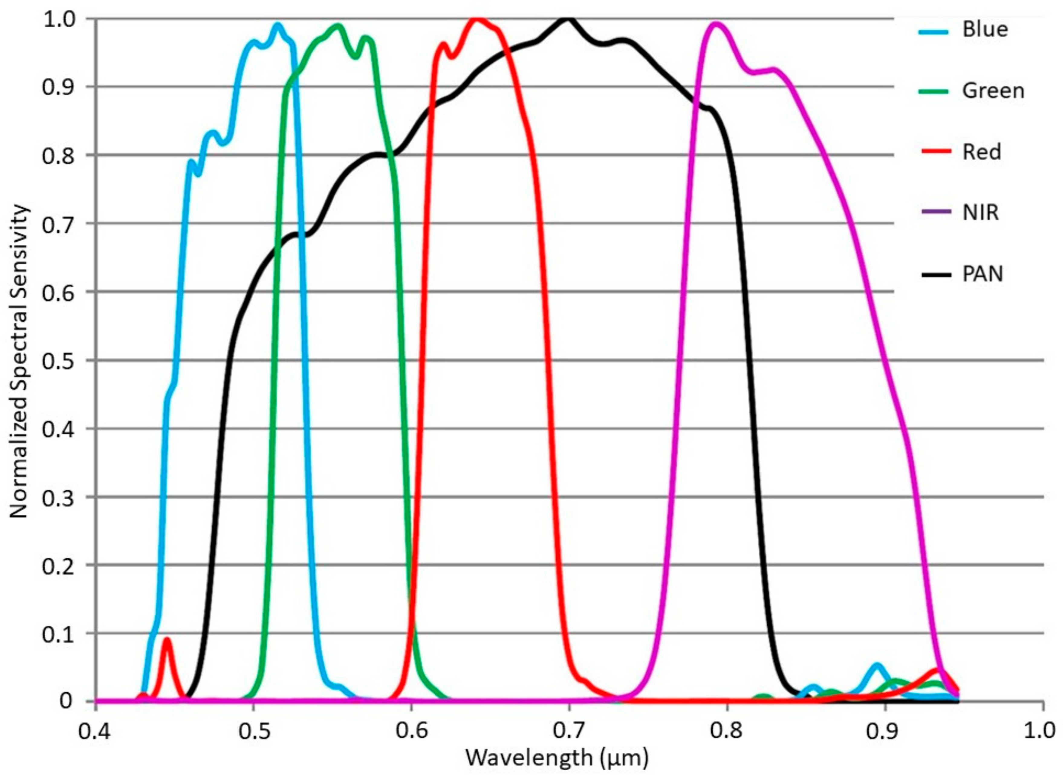
The Pléiades constellation is composed of two VHR optical Earth-imaging satellites named Pléiades-HR 1A (launched in December 2011) and Pléiades-HR 1B (launched in December 2012). These satellites of CNES (Centre National d’Études Spatiales), the Space Agency of France, provide coverage of the Earth’s surface with a repeat cycle of 26 days. Designed for civil and military users, the Pléiades system is suitable for emergency response and change detection [87]. Pléiades imagery consists of panchromatic and multispectral data. The former present a spatial resolution of 0.50 m, and the spectral range is 0.480–0.830 μm. The latter have resolution of 2.00 m and include four Multispectral bands: Blue (0.430–0.550 μm), Green (0.490–0.610 μm), Red (0.600–0.720 μm) and Near Infrared (0.750–0.950 μm) [88]. The spectral response associated with the Pléiades MS and PAN sensors is shown in Figure 1.
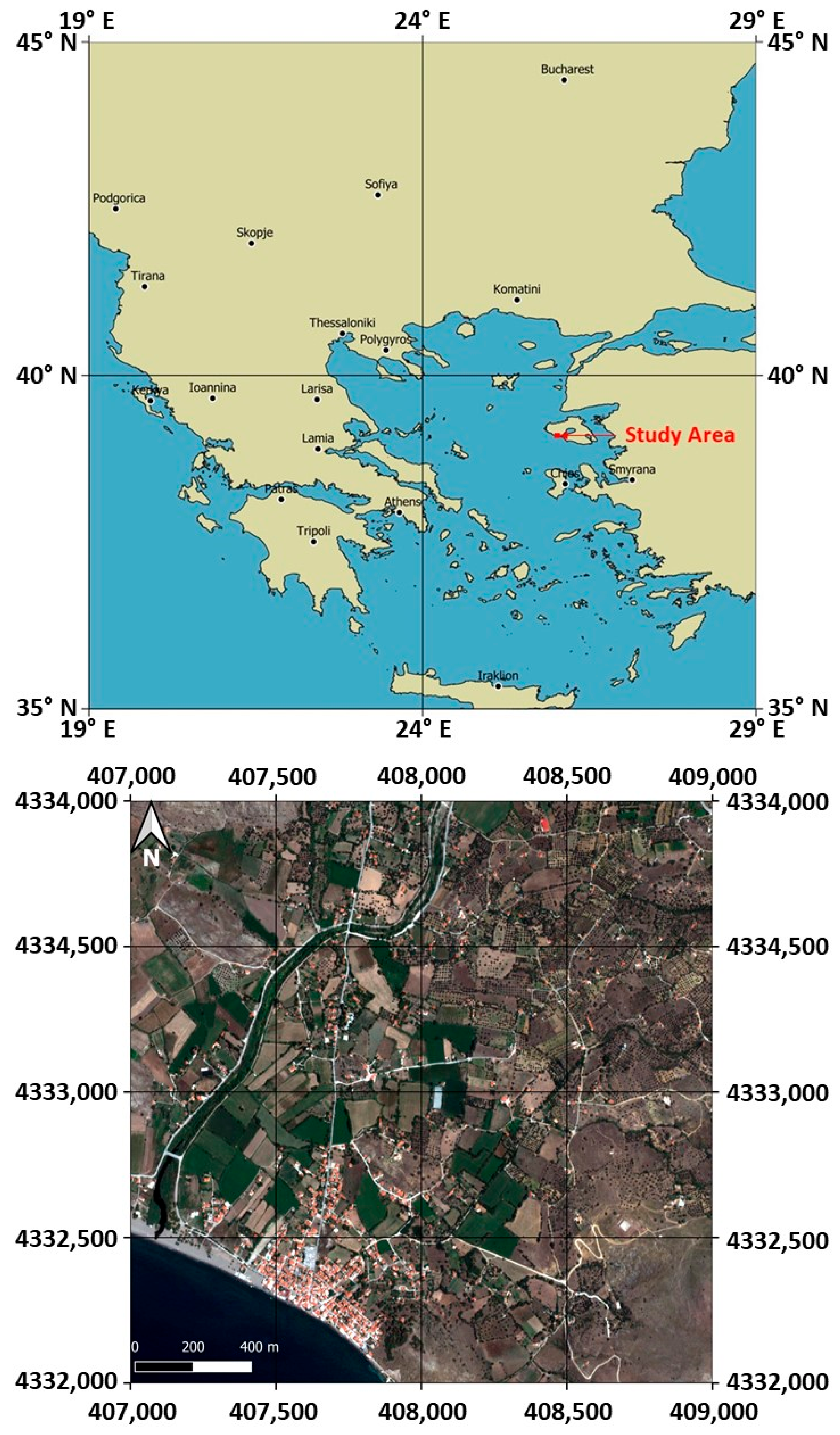
In this study, Pléiades-HR 1B imagery concerning the island of Lesbo (Greece) is considered. The whole scene was acquired on 1 July 2014. It has been made available free of charge by European Space Agency (ESA). The clip used for the experiments (Figure 2) extends 2000 m × 2000 m and is georeferenced in the UTM/WGS84 (Zone 35 N) coordinate system (Figure 2). Particularly, the area is included between coordinates East 407,000–409,000 m and North 4,332,000–4,334,000 m.
3.2. Implementation of Pan-Sharpening Methods in QGIS
QGIS is a free and open-source GIS software licensed under the GNU General Public License. It is the product of the Open Source Geospatial Foundation (OSGeo), and version 1.0 was released in 2009. Built in C++, it uses Python for scripting and plugins. It is commonly defined as user-friendly, fully functional and relatively lightweight. It runs on Windows, Linux, Unix, Mac OSX and Android and is integrated into OSGeo tools (GRASS, Saga, GDAL, etc.) [89].
QGIS has a graphical modeller built-in that can help to define the workflow of two or more operations and run it with a single invocation. GIS Workflows typically involve many steps, with each step generating intermediate output that is used by the next step. Using the graphical modeller, it is not necessary to run through the entire process again manually to change the input data or a parameter. In other terms, the model is executed as a single algorithm [90].
The following steps are required to create a model.
- Definition of necessary inputs. The inputs are added to the parameters window, so the user can set their values when executing the model. Because the model itself is an algorithm, the parameters window is generated automatically as it occurs with all the algorithms available in the processing framework.
- Definition of the workflow. The workflow is defined by adding algorithms and selecting how they use the input data of the model or the outputs created by other algorithms already in the model.
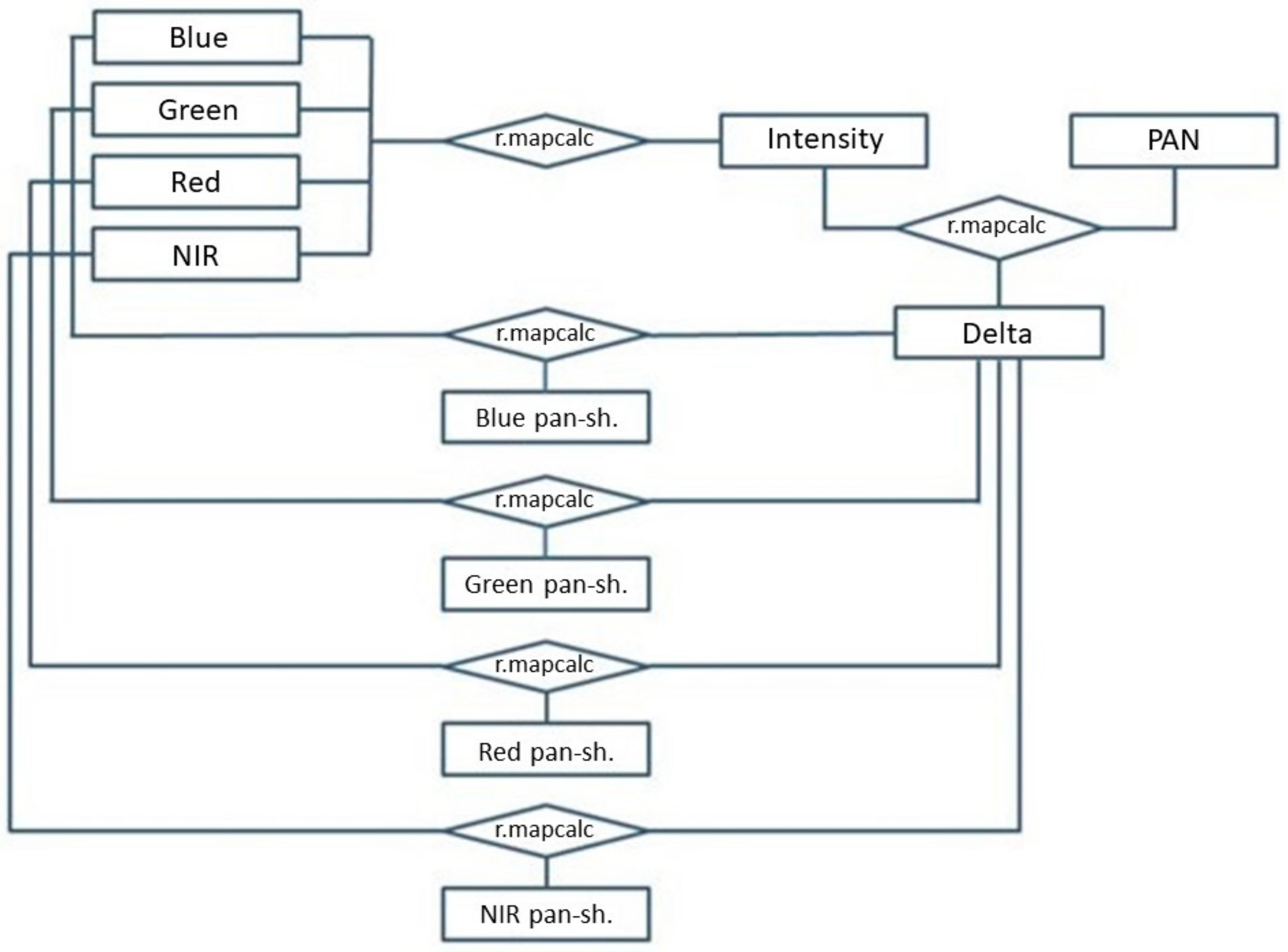
For example, to implement the IHS pan-sharpening method for Pléiades images, the workflow reported in Figure 3 has been created. All formulas reported in the previous subparagraph have been implemented using the algorithm named r.mapcalc [91] including in GRASS. Particularly, the workflow highlights that the user is asked to choose the images to which to apply the IHS method and the automatic procedure begins: using the algorithm r.mapcalc, the routine firstly implement formula (1) and then formula (2), finally generating the MS fused images.
3.3. Procedure Steps
Once the pan-sharpening algorithms and the calculation of the indices in QGIS have been implemented, the procedure is fully automated by following the steps below:
- Selection of the images to use in order to achieve pan-sharpening from the Pléiades image set;
- Application of the selected pan-sharpening methods among the 14 available ones;
- Visualization of the fusion products;
- Calculation of 7 different indices to evaluate the quality of the products;
- Comparison of quality indices, through an evaluation process based on the attribution of different weights, to detect the best-fused products.
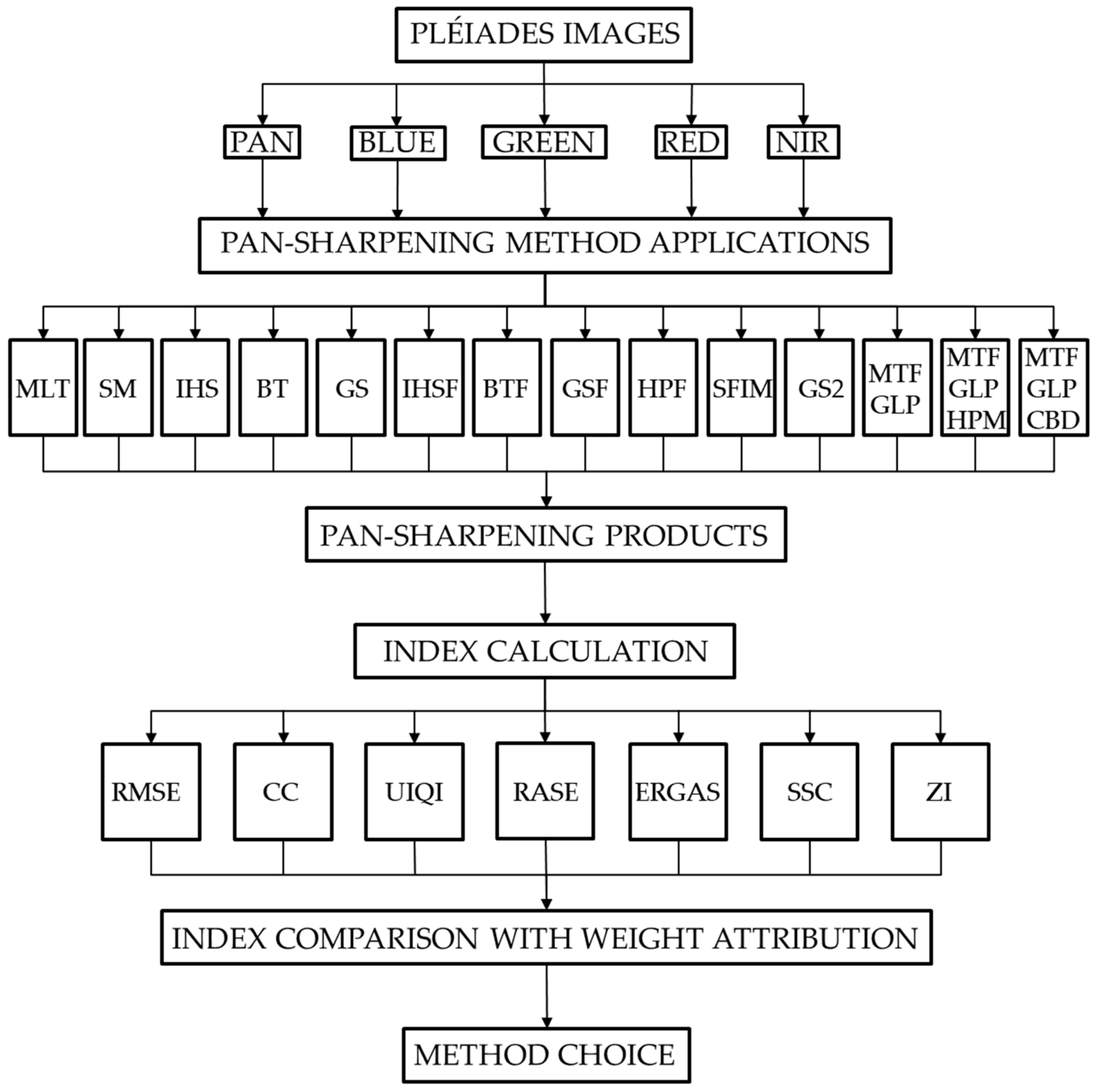
The above-described steps are reported in the flow-chart shown in Figure 4.
The process is created for the Pléiades dataset, but it is repeatable for any set of satellite images.
The weights assigned to each index can be freely chosen by the user based on the required needs. Finally, the best performing method is detected by multi-criteria analysis [92].
As the purpose of this manuscript is not to compare different pan-sharpening methods but to automate the image fusion process and support the choice of the best pan-sharpening method, we decided to repeat all operations manually in QGIS to have images produced in the usual way to compare with the automatic outputs. In this way, the accuracy of the proposed approach is evaluated.
4. Results and Discussion
Considering that the starting multispectral images are 4 and the methods implemented are 14, the implementation of our proposal generates 56 pan-sharpened images. The products obtained from the application of each method are quantitatively evaluated using the quality indices mentioned in Section 2.2. The results of these metrics are shown in the following tables (Table 1, Table 2, Table 3, Table 4, Table 5, Table 6, Table 7, Table 8, Table 9, Table 10, Table 11, Table 12, Table 13 and Table 14), one for each method.
Table 15 is a comparative table of all the methods (note: for each index, only the mean value is reported for an easier synoptic view).
However, the results highlight some significant aspects, as reported below.
Even if all spectral indices do not supply the same classification, underlying trends are evident. For example, the level of correlation between each pan-sharpened image and the corresponding original one is high in many cases, testifying to the effectiveness of the analysed method. The lowest values are usually obtained for the blue band as a consequence of the low level of overlap between the PAN sensor’s spectral response and the Blue sensor’s spectral response (Figure 1). In addition, all spectral indices supply the same result for the best performing method (MTF–GLP–CBD); however, they do not identify the same method as the weakest (i.e., BT for CC and MLT for ERGAS).
On the other hand, spatial indices provide a ranking that is in some respects different from that given by spectral indices. In fact, the best performing method in terms of spectral fidelity, MTF–GLP–CBD, supply poor results in terms of spatial fidelity. As testified by other studies [44,93], the improvement of the spatial quality of one image means the deterioration of the spectral quality and vice versa.
In light of the above considerations, a compromise must be sought in terms of spectral preservation and spatial enhancement to ensure good pan-sharpened products.
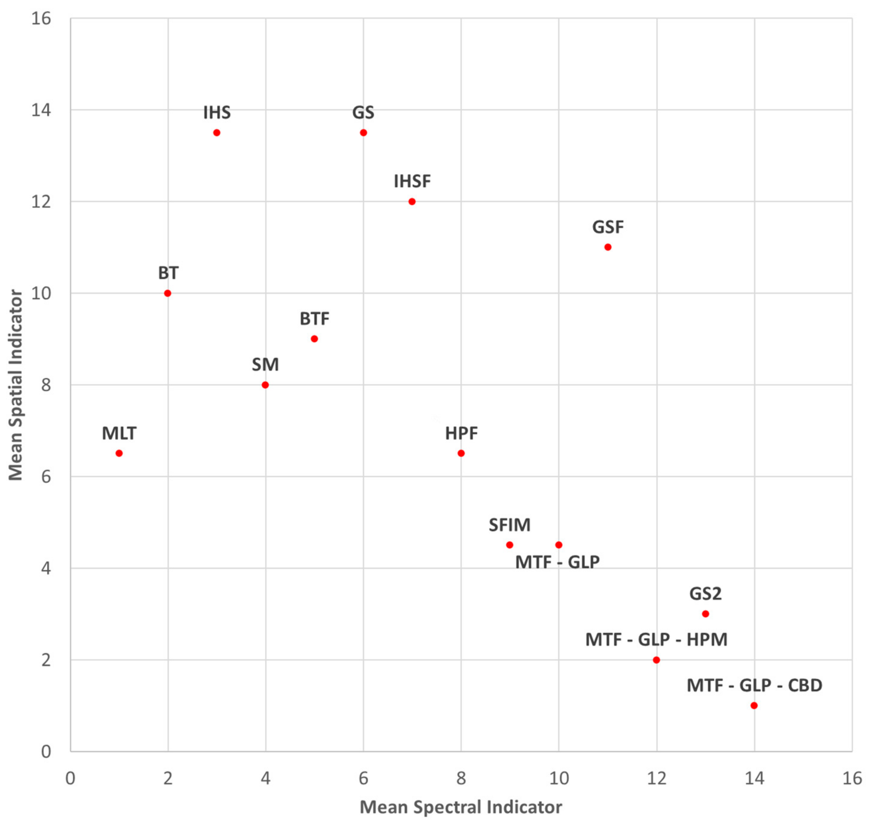
To better compare the results, we decided to assign a score to each method. In particular, as a first step, a ranking is made for the methods in consideration of each indicator, assigning a score from 1 to 14. The spectral indicators are then mediated between them, as well as the spatial indicators. Figure 5 shows the results obtained by each method taking into account the mean spectral indicator and the mean spatial indicator.
As the last step, a general ranking can be obtained by introducing weights for Mean Spectral Indicator and Mean Spatial Indicator. For example, using the same weight (0.5) for both indicators, the resulting classification is shown in Table 16.
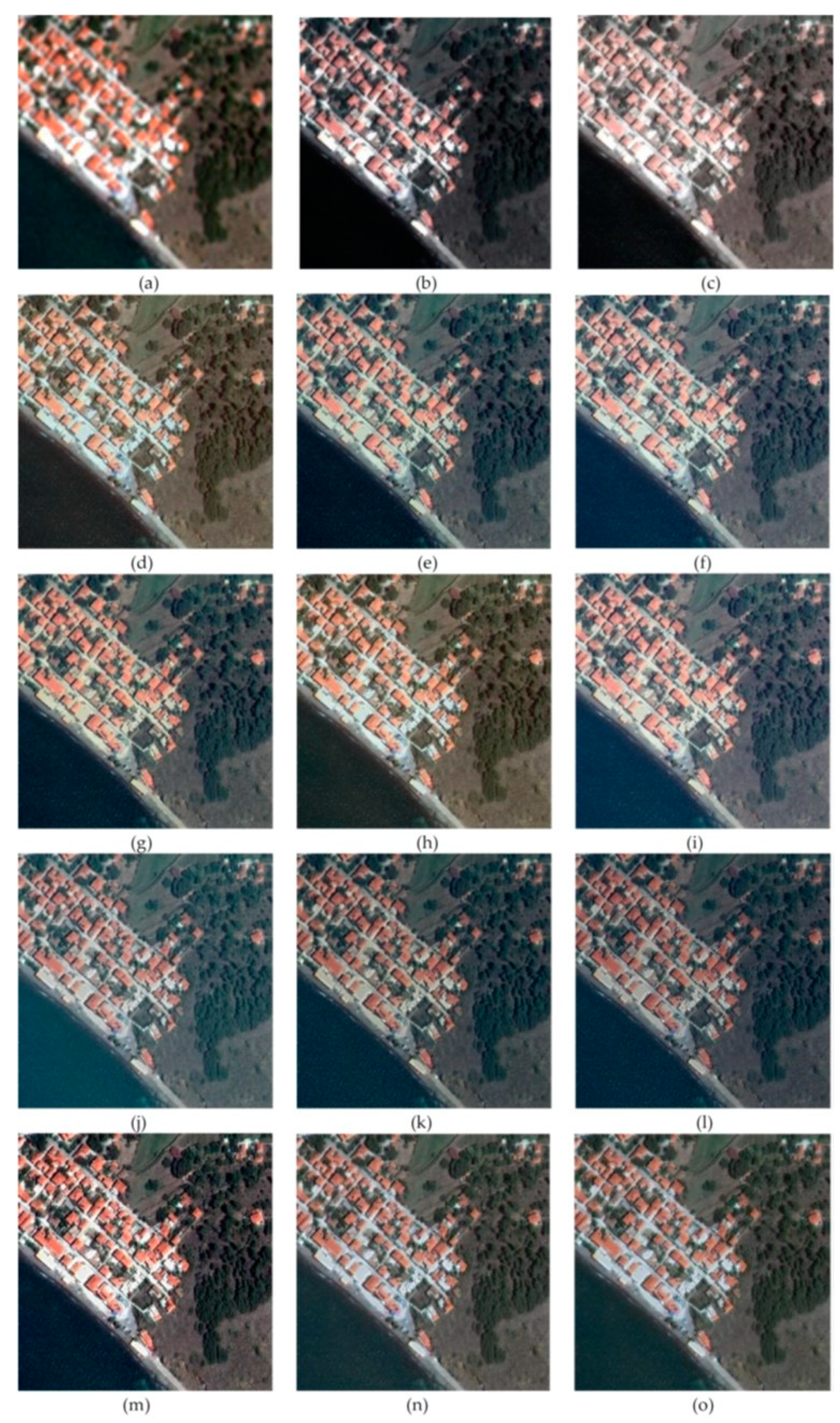
To give an idea of the quality of the derived images, Figure 6 shows the zoom of the RGB composition of the initial multispectral images as well as the zoom of the RGB composition of the multispectral pan-sharpened images obtained from each method.
Comparing these results by means of visual inspection, the increase of the geometric resolution as well as the level of the reliability of the obtained colours are evident. In some cases, e.g., for the images resulting from the GSF, the colours are correctly preserved, and the details injected by the panchromatic data are impressive. This result confirms the high performance certified for this method by our classification based on the Multi-criteria approach. In other cases, however, e.g., for the images deriving from the BTF or HPF, there is a lower level of fidelity to the original gradations of the colours. Finally, as in the case of SFIM-derived images, there is a loss of spatial detail that is not opportunely injected in the multispectral products.
All the operations conducted in an automated way by means of GIS tools were also executed in a non-automated way by the authors to test the exactness of the algorithms implemented in the graphical modeller. Particularly, for each method, the differences between the single multispectral pan-sharpened image obtained in an automated way and the corresponding one obtained in a non-automated way were calculated. The residuals were zero in every case. Ultimately, both products are perfectly coincident, and the proposed approach is positively tested, so it can be used as a valuable tool to deal with a critical aspect of pan-sharpening. In fact, according to [44], there is no single method or processing chain for image fusion: in order to obtain the best results, a good understanding of the principles of fusing operations and especially good knowledge of the data characteristics are compulsory. Since each method can give different performances in different situations, applications of several algorithms and comparison of the results are preferable. This approach is very demanding and time-consuming, so the automation of pan-sharpening methods using GIS basic functions proposed in this work enables the user to achieve the best results in a rapid, easy and effective way.
5. Conclusions
The work presented here analyses the possibility to apply pan-sharpening methods to Pléiades images by means of GIS basic functions, without using specific pan-sharpening tools. The free and open-source GIS software named QGIS was chosen for all applications carried out. Finally, 14 methods are automatically applied and compared using quality indices and multi-criteria analysis.
The results demonstrate that the transfer of the higher geometric resolution of panchromatic data to multispectral ones does not require specific tools because it can be implemented using filters and Map Algebra functions. QGIS software supplies the Raster calculator, a simple but powerful tool to support specific operations that are fundamentals for pan-sharpening method applications, i.e., direct and reverse transformations between RGB and IHS space, synthetic image production, co-variance estimation. This tool is also useful to calculate indices for a quantitative evaluation of the quality of the resulting pan-sharpened images. The whole process can be automatised using a graphical modeller to simplify the user’s task by reducing it to select data.
Since the best performing method cannot be fixed in an absolute way but rather depends on the characteristics of the scene, several algorithms must be compared to select one providing suitable results for a defined purpose each time. For evaluating the quality indices by means of multi-criteria analysis, weights can be introduced in accordance with the user needs, i.e., putting spatial requirements before spectral ones or vice versa. In other words, our proposal aids the user by giving the automatic execution of pan-sharpening methods but also supporting the choice of the best-fused products. For this reason, the calculation of quality indices and the comparison of their values are both necessary.
Concerning the future developments of this work, further applications will be focused on the possibility to integrate other pan-sharpening methods in order to increase the number of available options for the user. In addition, we will be mainly focused on the possibility to facilitate the choice of the best performing method, also supplying other results in an automatic way, i.e., feature extractions in sample area to compare them with known shape objects for accuracy estimation.
Author Contributions
C.P. has conceived the article and designed the experiments; E.A. and A.V. conducted the bibliographic research; C.P. organized data collection and supervised the GIS applications; E.A. and A.V. conducted the experiments on pan-sharpening applications; E.A. conducted the quality tests; C.P. designed the flow-charts of the graphical modeller; A.V. supervised the algorithm implementation; all authors took part in the result analysis and writing the paper. All authors have read and agreed to the published version of the manuscript.
Funding
This research was funded by the University of Naples “Parthenope”.
Acknowledgments
This paper presents results of experiments performed within a research project supported by the University of Naples “Parthenope”. The images used for the experiments have been made available free of charge by the European Space Agency (ESA). The authors wish to thank Theresa Gavin for supporting the revision of the English text of the manuscript. We also would like to give our sincere thanks to the editors and the reviewers for their useful suggestions and constructive comments for improving the quality of this article.
Conflicts of Interest
The authors declare no conflict of interest.
References
- Dardanelli, G.; Allegra, M.; Giammarresi, V.; Brutto, M.L.; Pipitone, C.; Baiocchi, V. Geomatic Methodologies for The Study of Teatro Massimo in Palermo (Italy). Int. Arch. Photogramm. Remote Sens. Spat. Inf. Sci. 2017, XLII-5/W1, 475–480. [Google Scholar] [CrossRef] [Green Version]
- Weng, Q. Modeling Urban Growth Effects on Surface Runoff with the Integration of Remote Sensing and GIS. Environ. Manag. 2001, 28, 737–748. [Google Scholar] [CrossRef] [PubMed]
- Xian, G.; Crane, M. Assessments of urban growth in the Tampa Bay watershed using remote sensing data. Remote Sens. Environ. 2005, 97, 203–215. [Google Scholar] [CrossRef]
- Kääb, A.; Paul, F.; Maisch, M.; Hoelzle, M.; Haeberli, W. The new remote-sensing-derived Swiss glacier inventory: II. First results. Ann. Glaciol. 2002, 34, 362–366. [Google Scholar] [CrossRef] [Green Version]
- Baumhoer, C.A.; Dietz, A.J.; Dech, S.; Kuenzer, C. Remote Sensing of Antarctic Glacier and Ice-Shelf Front Dynamics—A Review. Remote Sens. 2018, 10, 1445. [Google Scholar] [CrossRef] [Green Version]
- Helldén, U.; Tottrup, C. Regional desertification: A global synthesis. Glob. Planet. Chang. 2008, 64, 169–176. [Google Scholar] [CrossRef]
- Fu, B.; Shi, P.; Fu, H.; Ninomiya, Y.; Du, J. Geological Mapping Using Multispectral Remote Sensing Data in the Western China. In Proceedings of the 2019 IEEE International Geoscience and Remote Sensing Symposium, Yokohama, Japan, 28 July–2 August 2019; pp. 5583–5586. [Google Scholar]
- Ali, I.; Cawkwell, F.; Dwyer, E.; Barrett, B.; Green, S. Satellite remote sensing of grasslands: From observation to management. J. Plant Ecol. 2016, 9, 649–671. [Google Scholar] [CrossRef] [Green Version]
- Mardian, J. Evaluating the utility of remote sensing time series analysis for the identification of grassland conversions in Alberta, Canada. Master’s Thesis, University of Guelph, Guelph, ON, Canada, 2020. [Google Scholar]
- Giglio, L.; Loboda, T.; Roy, D.P.; Quayle, B.; Justice, C.O. An active-fire based burned area mapping algorithm for the MODIS sensor. Remote Sens. Environ. 2009, 113, 408–420. [Google Scholar] [CrossRef]
- De Araújo, F.M.; Ferreira, L.G. Satellite-based automated burned area detection: A performance assessment of the MODIS MCD45A1 in the Brazilian savanna. Int. J. Appl. Earth Obs. Geoinf. 2015, 36, 94–102. [Google Scholar] [CrossRef]
- Baiocchi, V.; Brigante, R.; Radicioni, F. Three-dimensional multispectral classification and its application to early seismic damage assessment. Ital. J. Remote Sens. 2010, 42, 49–65. [Google Scholar] [CrossRef]
- Baiocchi, V.; Brigante, R.; Dominici, D.; Milone, M.V.; Mormile, M.; Radicioni, F. Automatic three-dimensional features extraction: The case study of L’Aquila for collapse identification after April 06, 2009 earthquake. Eur. J. Remote Sens. 2014, 47, 413–435. [Google Scholar] [CrossRef]
- Chen, X.; Achilli, V.; Fabris, M.; Menin, A.; Monego, M.; Tessari, G.; Floris, M. Combining Sentinel-1 Interferometry and Ground-Based Geomatics Techniques for Monitoring Buildings Affected by Mass Movements. Remote Sens. 2021, 13, 452. [Google Scholar] [CrossRef]
- Fiaschi, S.; Fabris, M.; Floris, M.; Achilli, V. Estimation of land subsidence in deltaic areas through differential SAR inter-ferometry: The Po River Delta case study (Northeast Italy). Int. J. Remote Sens. 2018, 39, 8724–8745. [Google Scholar] [CrossRef]
- Specht, M.; Specht, C.; Lewicka, O.; Makar, A.; Burdziakowski, P.; Dąbrowski, P. Study on the Coastline Evolution in Sopot (2008–2018) Based on Landsat Satellite Imagery. J. Mar. Sci. Eng. 2020, 8, 464. [Google Scholar] [CrossRef]
- Maglione, P. Very High Resolution Optical Satellites: An Overview of the Most Commonly used. Am. J. Appl. Sci. 2016, 13, 91–99. [Google Scholar] [CrossRef] [Green Version]
- Maglione, P.; Parente, C.; Vallario, A. Pan-sharpening Worldview-2: IHS, Brovey and Zhang methods in comparison. Int. J. Eng. Technol. 2016, 8, 673–679. [Google Scholar]
- Arablouei, R. Fusing Multiple Multiband Images. J. Imaging 2018, 4, 118. [Google Scholar] [CrossRef] [Green Version]
- Garzelli, A.; Nencini, F.; Capobianco, L. Optimal MMSE Pan Sharpening of Very High Resolution Multispectral Images. IEEE Trans. Geosci. Remote Sens. 2008, 46, 228–236. [Google Scholar] [CrossRef]
- Li, X.-Z.; Wang, P.; Zang, Y.-B. Application of SPOT 5 data fusion on investigating the ecological environment of mining area. In Proceedings of the 2009 Joint Urban Remote Sensing Event, Shanghai, China, 20–22 May 2009; pp. 1–6. [Google Scholar] [CrossRef]
- Zhang, J. Multi-source remote sensing data fusion: Status and trends. Int. J. Image Data Fusion 2010, 1, 5–24. [Google Scholar] [CrossRef] [Green Version]
- Ghassemian, H. A review of remote sensing image fusion methods. Inf. Fusion 2016, 32, 75–89. [Google Scholar] [CrossRef]
- Sekrecka, A.; Kedzierski, M. Integration of Satellite Data with High Resolution Ratio: Improvement of Spectral Quality with Preserving Spatial Details. Sensors 2018, 18, 4418. [Google Scholar] [CrossRef] [Green Version]
- Kizel, F.; Benediktsson, J.A. Spatially Enhanced Spectral Unmixing Through Data Fusion of Spectral and Visible Images from Different Sensors. Remote Sens. 2020, 12, 1255. [Google Scholar] [CrossRef] [Green Version]
- Falchi, U. IT tools for the management of multi—Representation geographical information. Int. J. Eng. Technol. 2017, 7, 65–69. [Google Scholar] [CrossRef] [Green Version]
- Mohammed, N.Z.; Ghazi, A.; Mustafa, H.E. Positional accuracy testing of Google Earth. Int. J. Multidiscip. Sci. Eng. 2013, 4, 6–9. [Google Scholar]
- Shah, V.P.; Younan, N.H.; King, R.L. A novel method to evaluate the performance of pan-sharpening algorithms. In Proceedings of the Defense and Security Symposium, Orlando, FL, USA, 9 April 2017; Volume 6571, p. 657102. [Google Scholar]
- Byun, Y.; Choi, J.; Han, Y. An Area-Based Image Fusion Scheme for the Integration of SAR and Optical Satellite Imagery. IEEE J. Sel. Top. Appl. Earth Obs. Remote Sens. 2013, 6, 2212–2220. [Google Scholar] [CrossRef]
- Errico, A.; Angelino, C.V.; Cicala, L.; Persechino, G.; Ferrara, C.; Lega, M.; Vallario, A.; Parente, C.; Masi, G.; Gaetano, R.; et al. Detection of environmental hazards through the feature-based fusion of optical and SAR data: A case study in southern Italy. Int. J. Remote Sens. 2015, 36, 3345–3367. [Google Scholar] [CrossRef] [Green Version]
- Mohammadzadeh, A.; Tavakoli, A.; Valadan Zoej, M.J. Road extraction based on fuzzy logic and mathematical morphology from pan-sharpened ikonos images. Photogramm. Rec. 2006, 21, 44–60. [Google Scholar] [CrossRef]
- Phinzi, K.; Abriha, D.; Bertalan, L.; Holb, I.; Szabó, S. Machine Learning for Gully Feature Extraction Based on a Pan-Sharpened Multispectral Image: Multiclass vs. Binary Approach. ISPRS Int. J. Geo-Inf. 2020, 9, 252. [Google Scholar] [CrossRef] [Green Version]
- Tomlin, D.C. GIS and Cartographic Modeling; Prentice Hall: New Jersey, NJ, USA, 1990. [Google Scholar]
- Longley, P.A.; Goodchild, M.F.; Maguire, D.J.; Rhind, D.W. Geographic Information Systems and Science, 2nd ed.; John Wiley & Sons: New York, NY, USA, 2005. [Google Scholar]
- Pitney Bowes, Mapbasic, Version 17.0, User Guide 2018. Available online: https://www.pitneybowes.com/content/dam/support/software/product-documentation/public/mapinfo-mapbasic/v17-0-0/en-us/mapinfo-mapbasic-v17-0-0-user-guide.pdf (accessed on 25 September 2020).
- QGIS. Welcome to the QGIS Project! Qgis. 2016. Available online: http://www.qgis.org/ (accessed on 25 September 2020).
- Alparone, L.; Wald, L.; Chanussot, J.; Thomas, C.; Gamba, P.; Bruce, L.M. Comparison of Pansharpening Algorithms: Outcome of the 2006 GRS-S Data-Fusion Contest. IEEE Trans. Geosci. Remote Sens. 2007, 45, 3012–3021. [Google Scholar] [CrossRef] [Green Version]
- Pushparaj, J.; Hegde, A.V. Evaluation of pan-sharpening methods for spatial and spectral quality. Appl. Geomat. 2016, 9, 1–12. [Google Scholar] [CrossRef]
- Li, H.; Jing, L.; Wang, L.; Cheng, Q. Improved Pansharpening with Un-Mixing of Mixed MS Sub-Pixels near Boundaries between Vegetation and Non-Vegetation Objects. Remote Sens. 2016, 8, 83. [Google Scholar] [CrossRef] [Green Version]
- Yang, J.; Zhang, J. Pansharpening: From a generalised model perspective. Int. J. Image Data Fusion 2014, 5, 1–15. [Google Scholar] [CrossRef]
- Chavez, P.; Sides, S.C.; Anderson, J.A. Comparison of three different methods to merge multiresolution and multispectral data- Landsat TM and SPOT panchromatic. Photogramm. Eng. Remote Sens. 1991, 57, 295–303. [Google Scholar]
- Laben, C.A.; Brower, B.V. Process for Enhancing the Spatial Resolution of Multispectral Imagery Using Pan-Sharpening. United States Eastman Kodak Company (Rochester, New York). U.S. Patent 6,011,875, 4 January 2000. [Google Scholar]
- Basaeed, E.; Bhaskar, H.; Al-Mualla, M. Comparative analysis of pan-sharpening techniques on DubaiSat-1 images. In Proceedings of the 16th International Conference on Information Fusion, Istanbul, Turkey, 9–12 July 2013; pp. 227–234. [Google Scholar]
- Švab, A.; Oštir, K. High-resolution image fusion: Methods to preserve spectral and spatial resolution. Photogramm. Eng. Remote Sens. 2006, 72, 565–572. [Google Scholar] [CrossRef]
- Vrabel, J. Multispectral imagery advanced band sharpening study. Photogramm. Eng. Remote Sens. 2000, 66, 73–80. [Google Scholar]
- Liu, J.G. Smoothing Filter-based Intensity Modulation: A spectral preserve image fusion technique for improving spatial details. Int. J. Remote Sens. 2000, 21, 3461–3472. [Google Scholar] [CrossRef]
- Licciardi, G.; Vivone, G.; Mura, M.D.; Restaino, R.; Chanussot, J. Multi-resolution analysis techniques and nonlinear PCA for hybrid pansharpening applications. Multidimens. Syst. Signal Process. 2015, 27, 807–830. [Google Scholar] [CrossRef]
- Gonzalez-Audicana, M.; Saleta, J.; Catalan, R.; Garcia, R. Fusion of multispectral and panchromatic images using improved IHS and PCA mergers based on wavelet decomposition. IEEE Trans. Geosci. Remote Sens. 2004, 42, 1291–1299. [Google Scholar] [CrossRef]
- Nunez, J.; Otazu, X.; Fors, O.; Prades, A.; Pala, V.; Arbiol, R. Multiresolution-based image fusion with additive wavelet decomposition. IEEE Trans. Geosci. Remote Sens. 1999, 37, 1204–1211. [Google Scholar] [CrossRef] [Green Version]
- Aiazzi, B.; Alparone, L.; Baronti, S.; Garzelli, A. Context-driven fusion of high spatial and spectral resolution images based on oversampled multiresolution analysis. IEEE Trans. Geosci. Remote Sens. 2002, 40, 2300–2312. [Google Scholar] [CrossRef]
- Liu, Z.; Song, P.; Zhang, J.; Wang, J. Bidimensional Empirical Mode Decomposition for the fusion of multispectral and panchromatic images. Int. J. Remote Sens. 2007, 28, 4081–4093. [Google Scholar] [CrossRef]
- Tu, T.-M.; Su, S.-C.; Shyu, H.-C.; Huang, P.S. A new look at IHS-like image fusion methods. Inf. Fusion 2001, 2, 177–186. [Google Scholar] [CrossRef]
- Pohl, C.; Van Genderen, J.L. Review article Multisensor image fusion in remote sensing: Concepts, methods and applications. Int. J. Remote Sens. 1998, 19, 823–854. [Google Scholar] [CrossRef] [Green Version]
- Zhang, Y. Understanding image fusion. Photogramm. Eng. Remote Sens. 2004, 6, 657–661. [Google Scholar]
- Tu, T.-M.; Huang, P.S.; Hung, C.-L.; Chang, C.-P. A Fast Intensity–Hue–Saturation Fusion Technique with Spectral Adjustment for IKONOS Imagery. IEEE Geosci. Remote Sens. Lett. 2004, 1, 309–312. [Google Scholar] [CrossRef]
- Parente, C.; Santamaria, R. Increasing geometric resolution of data supplied by Quickbird multispectral sensors. Sens. Transducers 2013, 156, 111–115. [Google Scholar]
- Gharbia, R.; El Baz, A.H.; Hassanien, A.E.; Tolba, M.F. Remote Sensing Image Fusion Approach Based on Brovey and Wavelets Transforms. Intell. Fuzzy Tech. Big Data Anal. Decis. Mak. 2014, 303, 311–321. [Google Scholar] [CrossRef]
- Johnson, B. Effects of Pansharpening on Vegetation Indices. ISPRS Int. J. Geo-Inf. 2014, 3, 507–522. [Google Scholar] [CrossRef]
- Du, Q.; Younan, N.H.; King, R.; Shah, V.P. On the Performance Evaluation of Pan-Sharpening Techniques. IEEE Geosci. Remote Sens. Lett. 2007, 4, 518–522. [Google Scholar] [CrossRef]
- ESRI. What Is Map Algebra? Available online: https://desktop.arcgis.com/en/arcmap/latest/extensions/spatial-analyst/map-algebra/what-is-map-algebra.htm (accessed on 25 March 2021).
- Karakus, P.; Karabork, H. Effect of pansharpened image on some of pixel based and object based classification accuracy. Int. Arch. Photogramm. Remote Sens. Spat. Inf. Sci. 2006, 7, 235–239. [Google Scholar]
- Chavez, P.S., Jr.; Bowell, J.A. Comparison of the spectral information content of Landsat Thematic Mapper and SPOT for three different sites in the Phoenix, Arizona region. Photogramm. Eng. Remote Sens. 1988, 54, 1699–1708. [Google Scholar]
- Vivone, G.; Alparone, L.; Chanussot, J.; Mura, M.D.; Garzelli, A.; Licciardi, G.A.; Restaino, R.; Wald, L. A Critical Comparison Among Pansharpening Algorithms. IEEE Trans. Geosci. Remote Sens. 2015, 53, 2565–2586. [Google Scholar] [CrossRef]
- Pradines, D. Improving SPOT images size and multispectral resolution. In Earth Remote Sensing Using the Landsat Thermatic Mapper and SPOT Sensor Systems. Int. Soc. Optics Photonics 1986, 660, 98–102. [Google Scholar]
- Guo, L.J.; Moore, J.M. Pixel block intensity modulation: Adding spatial detail to TM band 6 thermal imagery. Int. J. Remote Sens. 1998, 19, 2477–2491. [Google Scholar] [CrossRef]
- Wald, L.; Ranchin, T. Liu ’Smoothing filter-based intensity modulation: A spectral preserve image fusion technique for improving spatial details. Int. J. Remote Sens. 2002, 23, 593–597. [Google Scholar] [CrossRef]
- Wald, L. Data Fusion: Definitions and Architectures: Fusion of Images of Different Spatial Resolutions; Les Presses de l’École des Mines: Paris, France, 2002. [Google Scholar]
- Burt, P.J.; Adelson, E.H. The Laplacian Pyramid as a Compact Image Code. IEEE Trans. Commun. 1983, 31, 532–540. [Google Scholar] [CrossRef]
- Aiazzi, B.; Baronti, S.; Selva, M. Image fusion through multiresolution oversampled decompositions. Image Fusion 2008, 27–66. [Google Scholar] [CrossRef]
- Aiazzi, B.; Alparone, L.; Baronti, S.; Pippi, I. Fusion of 18 m MOMS-2P and 30 m Landsat TM multispectral data by the generalized Laplacian pyramid. ISPRS Int. Arch. Photogramm. Remote Sens. 1999, 32, 116–122. [Google Scholar]
- Delleji, T.; Kallel, A.; Ben Hamida, A. Iterative scheme for MS image pansharpening based on the combination of multi-resolution decompositions. Int. J. Remote Sens. 2016, 37, 6041–6075. [Google Scholar] [CrossRef]
- Lee, J.; Lee, C. Fast and Efficient Panchromatic Sharpening. IEEE Trans. Geosci. Remote Sens. 2009, 48, 155–163. [Google Scholar] [CrossRef]
- Shahdoosti, H.R.; Ghassemian, H. Fusion of MS and PAN Images Preserving Spectral Quality. IEEE Geosci. Remote Sens. Lett. 2014, 12, 611–615. [Google Scholar] [CrossRef]
- Saroglu, E.; Bektas, F.; Musaoglu, N.; Goksel, C. Fusion of multisensory sensing data: Assessing the quality of resulting images. ISPRS Arch. 2004, 25, 575–579. [Google Scholar]
- Rahimzadeganasl, A.; Alganci, U.; Goksel, C. An Approach for the Pan Sharpening of Very High Resolution Satellite Images Using a CIELab Color Based Component Substitution Algorithm. Appl. Sci. 2019, 9, 5234. [Google Scholar] [CrossRef] [Green Version]
- Meng, X.; Li, J.; Shen, H.; Zhang, L.; Zhang, H. Pansharpening with a Guided Filter Based on Three-Layer Decomposition. Sensors 2016, 16, 1068. [Google Scholar] [CrossRef] [PubMed]
- Wang, Z.; Bovik, A.C. A universal image quality index. IEEE Signal Process. Lett. 2002, 9, 81–84. [Google Scholar] [CrossRef]
- Alparone, L.; Baronti, S.; Garzelli, A.; Nencini, F. A Global Quality Measurement of Pan-Sharpened Multispectral Imagery. IEEE Geosci. Remote Sens. Lett. 2004, 1, 313–317. [Google Scholar] [CrossRef]
- Nikolakopoulos, K.; Oikonomidis, D. Quality assessment of ten fusion techniques applied on Worldview-2. Eur. J. Remote Sens. 2015, 48, 141–167. [Google Scholar] [CrossRef]
- Garzelli, A.; Nencini, F. Hypercomplex Quality Assessment of Multi/Hyperspectral Images. IEEE Geosci. Remote Sens. Lett. 2009, 6, 662–665. [Google Scholar] [CrossRef]
- Sarp, G. Spectral and spatial quality analysis of pan-sharpening algorithms: A case study in Istanbul. Eur. J. Remote Sens. 2014, 47, 19–28. [Google Scholar] [CrossRef] [Green Version]
- Meinel, G.; Neubert, M. A comparison of segmentation programs for high resolution remote sensing data. Int. Arch. Photogramm. Remote Sens. 2014, 35, 1097–1105. [Google Scholar]
- Hegde, G.P.; Hegde, N.; Muralikrishna, V.D.I. Measurement of quality preservation of pan-sharpened image. Int. J. Eng. Res. Dev. 2012, 2, 12–17. [Google Scholar]
- Parente, C.; Pepe, M. Influence of the weights in IHS and Brovey methods for pan-sharpening WorldView-3 satellite images. Int. J. Eng. Technol. 2017, 6, 71–77. [Google Scholar] [CrossRef] [Green Version]
- Li, S.; Kwok, J.T.; Wang, Y. Using the discrete wavelet frame transform to merge Landsat TM and SPOT panchromatic images. Inf. Fusion 2002, 3, 17–23. [Google Scholar] [CrossRef]
- Zhou, J.; Civco, D.L.; Silander, J.A. A wavelet transform method to merge Landsat TM and SPOT panchromatic data. Int. J. Remote Sens. 1998, 19, 743–757. [Google Scholar] [CrossRef]
- Airbus Defence and Space Geo-Intelligence. Pléiades Spot the Detail. Available online: http://www.intelligence-airbusds.com/files/pmedia/public/r61_9_geo_011_pleiades_en_low.pdf (accessed on 25 March 2021).
- Gleyzes, M.A.; Perret, L.; Kubik, P. Pleiades system architecture and main performances. ISPRS Int. Arch. Photogramm. Remote Sens. Spat. Inf. Sci. 2012, XXXIX-B1, 537–542. [Google Scholar] [CrossRef] [Green Version]
- GRASS Development Team. GRASS GIS 7.9.dev Reference Manual. 2020. Available online: https://grass.osgeo.org/grass79/manuals/index.html (accessed on 25 March 2021).
- Gandhi, U. Automating Complex Workflows Using Processing Modeler, QGIS Tutorials. Available online: http://www.qgistutorials.com/it/docs/processing_graphical_modeler.html (accessed on 25 March 2021).
- Shapiro, M.; Westervelt, J.R. MAPCALC: An Algebra for GIS and Image Processing; Construction Engineering Research Lab: Champaign, IL, USA, 1994. [Google Scholar]
- Dodgson, J.S.; Spackman, M.; Pearman, A.; Phillips, L.D. Multi-Criteria Analysis: A Manual; Department for Communities and Local Government: London, UK, 2009.
- Amolins, K.; Zhang, Y.; Dare, P. Wavelet based image fusion techniques—An introduction, review and comparison. ISPRS J. Photogramm. Remote Sens. 2007, 62, 249–263. [Google Scholar] [CrossRef]
Figure 1.
Spectral response of the Pléiades multispectral (MS) and panchromatic (PAN) sensors.

Figure 2.
The study area: localization of Lesbo Island into Aegean Sea, in equirectangular projection and WGS84 geographic coordinates (upper); the RGB overview of the Pléiades images, in UTM/WGS84 plane coordinate (lower).
Figure 2.
The study area: localization of Lesbo Island into Aegean Sea, in equirectangular projection and WGS84 geographic coordinates (upper); the RGB overview of the Pléiades images, in UTM/WGS84 plane coordinate (lower).

Figure 3.
Workflow of the IHS pan-sharpening algorithm implementation in the graphical modeller based on r.mapcalc.
Figure 3.
Workflow of the IHS pan-sharpening algorithm implementation in the graphical modeller based on r.mapcalc.

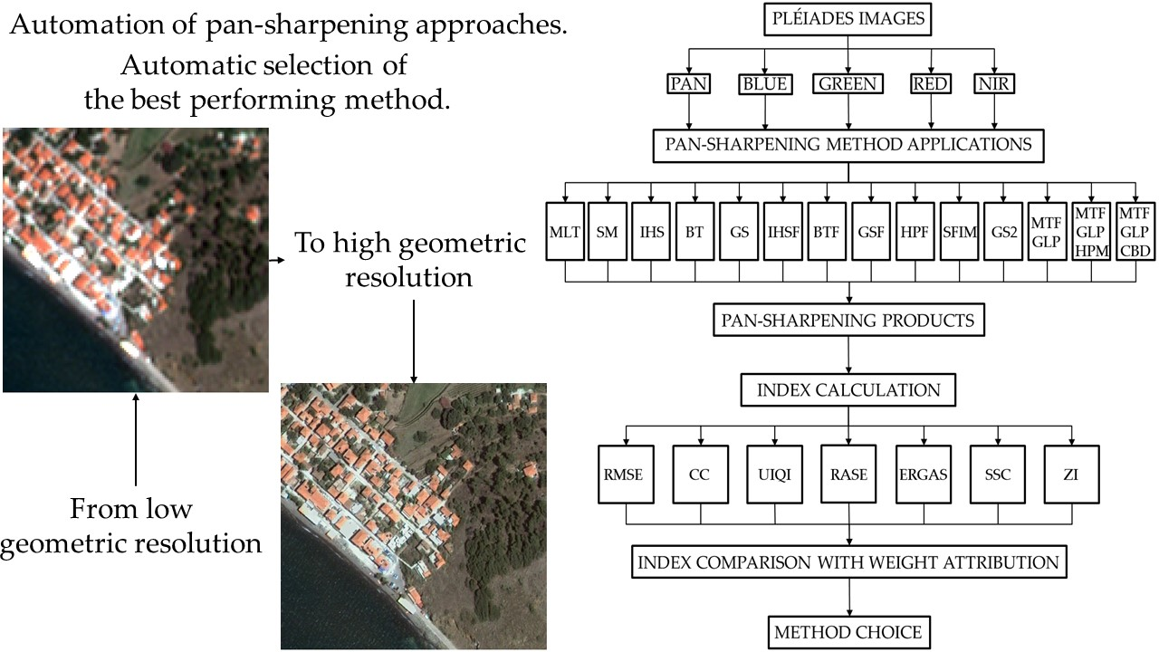
Figure 4.
Flow-chart of the automated procedure.

Figure 5.
Mean Spectral Indicator, on the x-axis, and Mean Spatial Indicator, on the y-axis, are plotted and compared.
Figure 5.
Mean Spectral Indicator, on the x-axis, and Mean Spatial Indicator, on the y-axis, are plotted and compared.

Figure 6.
Zoom of the RGB composition of the initial multispectral images (a) and zoom of the RGB composition of the multispectral pan-sharpened images obtained from each method, respectively: (b) MLT; (c) SM; (d) GS; (e) BT; (f) IHS; (g) BTF; (h) GSF; (i) IHSF; (j) HPF; (k) SFIM; (l) MTF–GLP–HPM; (m) MTF–GLP; (n) GS2; (o) MTF–GLP–CBD.


Table 1.
Quality indices for MLT pan-sharpening.
| MLT | RMSE | ERGAS | RASE | CC | CCM | UIQI | UIQIM | SCC | SCCM | ZI | ZIM |
|---|---|---|---|---|---|---|---|---|---|---|---|
| Blue | 44.855 | 7.791 | 29.089 | 0.909 | 0.925 | 0.573 | 0.721 | 0.930 | 0.901 | 0.834 | 0.763 |
| Green | 41.606 | 0.955 | 0.686 | 0.925 | 0.769 | ||||||
| Red | 39.566 | 0.954 | 0.801 | 0.875 | 0.657 | ||||||
| NIR | 38.640 | 0.881 | 0.824 | 0.875 | 0.792 |
Table 2.
Quality indices for SM pan-sharpening.
| SM | RMSE | ERGAS | RASE | CC | CCM | UIQI | UIQIM | SCC | SCCM | ZI | ZIM |
|---|---|---|---|---|---|---|---|---|---|---|---|
| Blue | 45.980 | 5.927 | 24.090 | 0.889 | 0.932 | 0.867 | 0.916 | 0.961 | 0.937 | 0.859 | 0.798 |
| Green | 36.699 | 0.947 | 0.941 | 0.968 | 0.814 | ||||||
| Red | 17.404 | 0.957 | 0.949 | 0.941 | 0.735 | ||||||
| NIR | 21.101 | 0.934 | 0.908 | 0.878 | 0.782 |
Table 3.
Quality indices for GS pan-sharpening.
| GS | RMSE | ERGAS | RASE | CC | CCM | UIQI | UIQIM | SCC | SCCM | ZI | ZIM |
|---|---|---|---|---|---|---|---|---|---|---|---|
| Blue | 11.440 | 3.399 | 12.858 | 0.928 | 0.934 | 0.911 | 0.913 | 0.890 | 0.884 | 0.915 | 0.908 |
| Green | 15.846 | 0.921 | 0.894 | 0.957 | 0.960 | ||||||
| Red | 21.795 | 0.925 | 0.900 | 0.930 | 0.948 | ||||||
| NIR | 18.694 | 0.963 | 0.947 | 0.757 | 0.808 |
Table 4.
Quality indices for BT pan-sharpening.
| BT | RMSE | ERGAS | RASE | CC | CCM | UIQI | UIQIM | SCC | SCCM | ZI | ZIM |
|---|---|---|---|---|---|---|---|---|---|---|---|
| Blue | 17.665 | 3.314 | 12.906 | 0.835 | 0.919 | 0.777 | 0.890 | 0.946 | 0.883 | 0.960 | 0.889 |
| Green | 17.685 | 0.915 | 0.879 | 0.963 | 0.963 | ||||||
| Red | 17.599 | 0.966 | 0.955 | 0.889 | 0.847 | ||||||
| NIR | 16.757 | 0.959 | 0.948 | 0.732 | 0.787 |
Table 5.
Quality indices for IHS pan-sharpening.
| IHS | RMSE | ERGAS | RASE | CC | CCM | UIQI | UIQIM | SCC | SCCM | ZI | ZIM |
|---|---|---|---|---|---|---|---|---|---|---|---|
| Blue | 16.948 | 3.215 | 12.548 | 0.856 | 0.922 | 0.817 | 0.898 | 0.921 | 0.886 | 0.966 | 0.905 |
| Green | 16.948 | 0.911 | 0.880 | 0.960 | 0.968 | ||||||
| Red | 16.948 | 0.953 | 0.939 | 0.913 | 0.899 | ||||||
| NIR | 16.948 | 0.969 | 0.956 | 0.750 | 0.788 |
Table 6.
Quality indices for BTF pan-sharpening.
| BTF | RMSE | ERGAS | RASE | CC | CCM | UIQI | UIQIM | SCC | SCCM | ZI | ZIM |
|---|---|---|---|---|---|---|---|---|---|---|---|
| Blue | 18.384 | 3.158 | 12.435 | 0.846 | 0.922 | 0.796 | 0.897 | 0.920 | 0.871 | 0.949 | 0.888 |
| Green | 16.481 | 0.918 | 0.887 | 0.950 | 0.957 | ||||||
| Red | 14.599 | 0.967 | 0.957 | 0.883 | 0.852 | ||||||
| NIR | 18.150 | 0.958 | 0.949 | 0.733 | 0.793 |
Table 7.
Quality indices for GSF pan-sharpening.
| GSF | RMSE | ERGAS | RASE | CC | CCM | UIQI | UIQIM | SCC | SCCM | ZI | ZIM |
|---|---|---|---|---|---|---|---|---|---|---|---|
| Blue | 10.108 | 3.111 | 11.699 | 0.944 | 0.943 | 0.933 | 0.929 | 0.861 | 0.868 | 0.884 | 0.895 |
| Green | 14.184 | 0.934 | 0.914 | 0.940 | 0.943 | ||||||
| Red | 19.727 | 0.935 | 0.918 | 0.915 | 0.940 | ||||||
| NIR | 18.097 | 0.961 | 0.950 | 0.756 | 0.814 |
Table 8.
Quality indices for IHSF pan-sharpening.
| IHSF | RMSE | ERGAS | RASE | CC | CCM | UIQI | UIQIM | SCC | SCCM | ZI | ZIM |
|---|---|---|---|---|---|---|---|---|---|---|---|
| Blue | 16.304 | 3.092 | 11.935 | 0.864 | 0.925 | 0.830 | 0.905 | 0.896 | 0.873 | 0.957 | 0.903 |
| Green | 16.304 | 0.914 | 0.888 | 0.946 | 0.963 | ||||||
| Red | 16.304 | 0.955 | 0.944 | 0.903 | 0.900 | ||||||
| NIR | 16.304 | 0.967 | 0.959 | 0.749 | 0.794 |
Table 9.
Quality indices for HPF pan-sharpening.
| HPF | RMSE | ERGAS | RASE | CC | CCM | UIQI | UIQIM | SCC | SCCM | ZI | ZIM |
|---|---|---|---|---|---|---|---|---|---|---|---|
| Blue | 15.998 | 3.034 | 11.914 | 0.864 | 0.920 | 0.832 | 0.904 | 0.798 | 0.823 | 0.918 | 0.874 |
| Green | 15.998 | 0.906 | 0.886 | 0.887 | 0.916 | ||||||
| Red | 15.998 | 0.951 | 0.944 | 0.862 | 0.857 | ||||||
| NIR | 15.998 | 0.958 | 0.956 | 0.747 | 0.803 |
Table 10.
Quality indices for SFIM pan-sharpening.
| SFIM | RMSE | ERGAS | RASE | CC | CCM | UIQI | UIQIM | SCC | SCCM | ZI | ZIM |
|---|---|---|---|---|---|---|---|---|---|---|---|
| Blue | 17.127 | 3.022 | 12.052 | 0.850 | 0.918 | 0.812 | 0.902 | 0.793 | 0.820 | 0.909 | 0.857 |
| Green | 15.751 | 0.909 | 0.890 | 0.884 | 0.905 | ||||||
| Red | 14.314 | 0.962 | 0.956 | 0.856 | 0.807 | ||||||
| NIR | 17.421 | 0.950 | 0.948 | 0.749 | 0.807 |
Table 11.
Quality indices for MTF-GLP-HPM pan-sharpening.
| MTF-GLP-HPM | RMSE | ERGAS | RASE | CC | CCM | UIQI | UIQIM | SCC | SCCM | ZI | ZIM |
|---|---|---|---|---|---|---|---|---|---|---|---|
| Blue | 15.578 | 2.743 | 10.957 | 0.863 | 0.927 | 0.836 | 0.916 | 0.790 | 0.816 | 0.888 | 0.853 |
| Green | 14.289 | 0.920 | 0.907 | 0.885 | 0.905 | ||||||
| Red | 12.962 | 0.969 | 0.965 | 0.851 | 0.821 | ||||||
| NIR | 15.832 | 0.958 | 0.957 | 0.737 | 0.797 |
Table 12.
Quality indices for MTF-GLP pan-sharpening.
| MTF-GLP | RMSE | ERGAS | RASE | CC | CCM | UIQI | UIQIM | SCC | SCCM | ZI | ZIM |
|---|---|---|---|---|---|---|---|---|---|---|---|
| Blue | 14.410 | 2.733 | 10.733 | 0.880 | 0.931 | 0.857 | 0.920 | 0.794 | 0.818 | 0.900 | 0.867 |
| Green | 14.410 | 0.918 | 0.905 | 0.886 | 0.914 | ||||||
| Red | 14.410 | 0.960 | 0.955 | 0.856 | 0.864 | ||||||
| NIR | 14.410 | 0.965 | 0.964 | 0.734 | 0.791 |
Table 13.
Quality indices for GS2 pan-sharpening.
| GS2 | RMSE | ERGAS | RASE | CC | CCM | UIQI | UIQIM | SCC | SCCM | ZI | ZIM |
|---|---|---|---|---|---|---|---|---|---|---|---|
| Blue | 7.999 | 2.651 | 10.265 | 0.967 | 0.954 | 0.960 | 0.948 | 0.784 | 0.821 | 0.748 | 0.817 |
| Green | 11.678 | 0.949 | 0.940 | 0.885 | 0.841 | ||||||
| Red | 16.158 | 0.950 | 0.942 | 0.862 | 0.860 | ||||||
| NIR | 17.277 | 0.951 | 0.949 | 0.753 | 0.820 |
Table 14.
Quality indices for MTF-GLP-CBD pan-sharpening.
| MTF-GLP-CBD | RMSE | ERGAS | RASE | CC | CCM | UIQI | UIQIM | SCC | SCCM | ZI | ZIM |
|---|---|---|---|---|---|---|---|---|---|---|---|
| Blue | 7.061 | 2.349 | 9.077 | 0.975 | 0.964 | 0.971 | 0.960 | 0.776 | 0.813 | 0.751 | 0.817 |
| Green | 10.375 | 0.959 | 0.954 | 0.882 | 0.852 | ||||||
| Red | 14.410 | 0.960 | 0.955 | 0.856 | 0.864 | ||||||
| NIR | 15.131 | 0.962 | 0.961 | 0.737 | 0.800 |
Table 15.
Quality indices comparison of all the pan-sharpening methods.
| METHOD | RMSEM | ERGAS | RASE | CCM | UIQIM | SCCM | ZIM |
|---|---|---|---|---|---|---|---|
| MLT | 41.167 | 7.791 | 29.089 | 0.925 | 0.721 | 0.901 | 0.763 |
| SM | 30.296 | 5.927 | 24.090 | 0.932 | 0.916 | 0.937 | 0.798 |
| GS | 16.944 | 3.399 | 12.858 | 0.934 | 0.913 | 0.884 | 0.908 |
| BT | 17.427 | 3.314 | 12.906 | 0.919 | 0.890 | 0.883 | 0.889 |
| IHS | 16.948 | 3.215 | 12.548 | 0.922 | 0.898 | 0.886 | 0.905 |
| BTF | 15.853 | 2.953 | 11.604 | 0.922 | 0.907 | 0.871 | 0.888 |
| IHSF | 15.103 | 2.865 | 10.969 | 0.926 | 0.915 | 0.873 | 0.903 |
| GSF | 13.404 | 2.707 | 10.022 | 0.952 | 0.945 | 0.868 | 0.895 |
| SFIM | 14.110 | 2.639 | 10.545 | 0.930 | 0.921 | 0.820 | 0.857 |
| HPF | 13.766 | 2.611 | 10.254 | 0.920 | 0.910 | 0.823 | 0.874 |
| MTFGLP | 13.836 | 2.588 | 10.323 | 0.929 | 0.922 | 0.818 | 0.867 |
| MTF–GLP–HPM | 12.965 | 2.459 | 9.659 | 0.938 | 0.933 | 0.816 | 0.853 |
| GS2 | 10.944 | 2.190 | 8.457 | 0.969 | 0.966 | 0.821 | 0.817 |
| MTF–GLP–CBD | 9.567 | 1.911 | 7.377 | 0.977 | 0.976 | 0.813 | 0.817 |
Table 16.
Ranking of the pan-sharpening methods.
| Method | Ranking |
|---|---|
| GSF | 1° |
| GS | 2° |
| IHSF | 3° |
| IHS | 4° |
| GS2 | 5° |
| MTF–GLP–CBD | 6° |
| MTF–GLP | 7° |
| HPF | 7° |
| MTF–GLP–HPM | 9° |
| BTF | 9° |
| SFIM | 11° |
| BT | 12° |
| SM | 12° |
| MLT | 14° |
Publisher’s Note: MDPI stays neutral with regard to jurisdictional claims in published maps and institutional affiliations. |
© 2021 by the authors. Licensee MDPI, Basel, Switzerland. This article is an open access article distributed under the terms and conditions of the Creative Commons Attribution (CC BY) license (https://creativecommons.org/licenses/by/4.0/).
Share and Cite
MDPI and ACS Style
Alcaras, E.; Parente, C.; Vallario, A. Automation of Pan-Sharpening Methods for Pléiades Images Using GIS Basic Functions. Remote Sens. 2021, 13, 1550. https://0-doi-org.brum.beds.ac.uk/10.3390/rs13081550
AMA Style
Alcaras E, Parente C, Vallario A. Automation of Pan-Sharpening Methods for Pléiades Images Using GIS Basic Functions. Remote Sensing. 2021; 13(8):1550. https://0-doi-org.brum.beds.ac.uk/10.3390/rs13081550
Chicago/Turabian StyleAlcaras, Emanuele, Claudio Parente, and Andrea Vallario. 2021. "Automation of Pan-Sharpening Methods for Pléiades Images Using GIS Basic Functions" Remote Sensing 13, no. 8: 1550. https://0-doi-org.brum.beds.ac.uk/10.3390/rs13081550
Note that from the first issue of 2016, this journal uses article numbers instead of page numbers. See further details here.