
New Biomass Estimates for Chaparral-Dominated Southern California Landscapes


1
RedCastle Resources, Inc., Contractor to: USDA Forest Service Western Wildlands Environmental Threat Assessment Center (WETAC), Bend, OR 97703, USA
2
Department of Environmental Science and Policy, University of California-Davis, 1023, Davis, CA 95616, USA
3
Centre for Biological Sciences, University of Southampton, Southampton SO17 1BJ, UK
*
Author to whom correspondence should be addressed.
Remote Sens. 2021, 13(8), 1581; https://0-doi-org.brum.beds.ac.uk/10.3390/rs13081581
Submission received: 17 March 2021
/
Revised: 9 April 2021
/
Accepted: 11 April 2021
/
Published: 19 April 2021
(This article belongs to the Special Issue Earth Observations for Biodiversity and Ecosystems of Mediterranean-Type Climate Regions)
Abstract
:Chaparral shrublands are the dominant wildland vegetation type in Southern California and the most extensive ecosystem in the state. Disturbance by wildfire and climate change have created a dynamic landscape in which biomass mapping is key in tracking the ability of chaparral shrublands to sequester carbon. Despite this importance, most national and regional scale estimates do not account for shrubland biomass. Employing plot data from several sources, we built a random forest model to predict aboveground live biomass in Southern California using remote sensing data (Landsat Normalized Difference Vegetation Index (NDVI)) and a suite of geophysical variables. By substituting the NDVI and precipitation predictors for any given year, we were able to apply the model to each year from 2000 to 2019. Using a total of 980 field plots, our model had a k-fold cross-validation R2 of 0.51 and an RMSE of 3.9. Validation by vegetation type ranged from R2 = 0.17 (RMSE = 9.7) for Sierran mixed-conifer to R2 = 0.91 (RMSE = 2.3) for sagebrush. Our estimates showed an improvement in accuracy over two other biomass estimates that included shrublands, with an R2 = 0.82 (RMSE = 4.7) compared to R2 = 0.068 (RMSE = 6.7) for a global biomass estimate and R2 = 0.29 (RMSE = 5.9) for a regional biomass estimate. Given the importance of accurate biomass estimates for resource managers, we calculated the mean year 2010 shrubland biomasses for the four national forests that ranged from 3.5 kg/m2 (Los Padres) to 2.3 kg/m2 (Angeles and Cleveland). Finally, we compared our estimates to field-measured biomasses from the literature summarized by shrubland vegetation type and age class. Our model provides a transparent and repeatable method to generate biomass measurements in any year, thereby providing data to track biomass recovery after management actions or disturbances such as fire.
1. Introduction
Evergreen sclerophyllous shrubland covers 9% of the state of California, half of which is located in the Mediterranean-type climate ecosystems of Southern California, notably in the chaparral shrublands in the Transverse and Peninsular range foothills [1]. Large topographic and precipitation gradients have resulted in tremendous regional species richness. While the rich plant diversity of these chaparral shrublands contribute to California’s Floristic Province status as a biodiversity hotspot, they also provide habitat for nearly 400 species of vertebrate fauna and provide multiple ecosystem services [2,3]. One of these services, albeit not widely recognized compared to forest landscapes, is the contribution shrublands make to climate mitigation through carbon storage and sustained carbon sequestration. Studies show old-growth chaparral shrublands to be a significant sink for carbon and, consequently, an important component of the global carbon budget [4,5].
The productivity of shrubland vegetation, and associated biomass and carbon storage, is related to environmental factors including distance to the coast, elevation, aspect, and the climatic water deficit. These environmental factors are reflected in plant communities with different species compositions. Dry, south-facing slopes (or rocky areas with shallow soils) are dominated by chamise chaparral (Adenostoma fasciculatum); less xeric, north-facing slopes (or areas with deeper soils) host mixed chaparral with a variety of species including ceanothus (Ceanothus spp.), manzanita (Arctostaphylos spp.), and scrub oak (Quercus berberidifolia); coastal areas are dominated by a single often locally endemic species of Ceanothus or Arctostaphylos [1,6]. Understanding patterns of shrubland productivity is important for resource managers given the relationship between productivity (and available fuels) and susceptibility of shrublands to large fires [7].
Disturbances, such as wildfire, are a major ecological factor in Southern California, with major fire years burning hundreds of thousands of hectares, causing extensive damage to homes and property, the loss of human lives, and millions of dollars spent in fire suppression costs [8,9,10]. This has been particularly poignant in recent decades, as Southern California has experienced several multi-year droughts, including the 2012–2017 drought which resulted in significant mortality in mature chaparral stands [11], consequently increasing future fire risk. During a wildfire, the combustion of living vegetation and dead fuel result in an initial release of large amounts of carbon [12,13]. Where the fire return interval of shrublands approximates the historic fire return interval (average 55 years for low-elevation shrubland) [8,14,15], shrub cover recovers after 10–14 years, while biomass keeps accumulating [16,17]. However, in many areas, the fire return interval has decreased, often in conjunction with an increase in non-native plant species, drought, and nitrogen deposition [18,19,20]. Under these conditions, post-fire biomass recovery can be impeded and, in some cases, may result in type conversion from native shrubland to non-native grassland [20].
Despite recognition of the importance of chaparral shrublands in ecosystem carbon budgets, there are few published methods for assessing the biomass of this vegetation type at the landscape scale and even fewer that can consistently be applied before and after disturbances such as wildfire. Regional and national biomass estimates often focus on forested lands only [21,22] where the amount of biomass in shrublands is considered negligible compared to forests at these spatial scales. However, given that chaparral shrublands cover nearly 3 million hectares (ha) in the state of California, their role in carbon sequestration should not be underestimated [23]. Mature chaparral shrublands capture and store substantial amounts of carbon aboveground while many resprouting species of chaparral are characterized by deep roots with large belowground carbon stores [24,25].
At the national scale, the foremost program for mapping biomass and combustible material (fuel) on wildlands is LANDFIRE, a cooperative program between the US Department of the Interior and the US Department of Agriculture Forest Service (USFS). However, often, these fuel mapping products are difficult to crosswalk into meaningful biomass estimates, as they focus on dead rather than live vegetation to inform fire behavior models.
Alternatively, at a finer scale, a few studies have assessed pre- and post-fire biomass in shrublands [26], although most have focused on a spatially and temporally limited number of plots, and the results are often not applicable beyond the immediate extent of the study. Studies at fine spatial scales can be dominated by site variability that obscures the detection of temporal trends or they have been undertaken at temporal scales and are unable to account for the influence of previous fire history and frequency.
This data gap is particularly important for land management agencies like the USFS that manage large areas of shrubland; for example, the four national forests in Southern California contain an average of 66% shrubland. Estimating the amount of biomass (and associated carbon storage) on federal lands and the effects of wildfire and management activities (e.g., fuel reduction) are critical components of resource management. Moreover, in instances when native shrubland fails to reestablish after fire it can alter the future risk and severity of fires [27], underscoring the importance of a readily available method for assessing biomass in planning activities. Timely estimates using a transparent, repeatable methodology of the impacts of wildfire on carbon storage can contribute to environmental damage assessments, while understanding how biomass recovers to pre-fire levels is important for managers given the connection between restoring vegetation cover and providing critical ecosystem services such as sediment erosion regulation [28].
Remote sensing has been shown to provide spatially explicit estimates of biomass in Mediterranean-type climate regions, over a variety of spatial and temporal scales [29]. The Landsat program (4, 5, 7, and 8) (www.landsat.usgs.gov/, accessed on 20 August 2019), in particular, offers a deep temporal stack (nearly 40 years) of images collected on average every 16 days, and at a 30 m spatial resolution, it is well-suited for monitoring heterogeneous shrublands at the landscape scale [30,31]. Spectral vegetation indices have been shown to be sensitive for detecting changes in shrubland vegetation and biomass. The Normalized Difference Vegetation Index (NDVI) was successfully used to estimate coastal shrubland biomass [32], dwarf shrub biomass [33], and to predict biomass using models that combine NDVI and precipitation data [34] in the Mediterranean Basin. Storey et al. (2016) found that NDVI and the normalized burn ratio (NBR) provided statistically significant indications of post-fire recovery two to three decades post-fire in Southern California. In other studies, the Enhanced Vegetation Index (EVI) has successfully assessed vegetation recovery post-fire on Mount Carmel, Israel [35], and in Southern California [26].
In this study, we developed a method to map biomass annually using vegetation indices derived from Landsat TM/ETM+/OLI instrument data (onboard Landsat 5, 7, and 8, respectively) and precipitation data specific to the year, resulting in a stack of biomass raster layers for the years 2000–2019. Specifically, we (1) created a random forest model using vegetation indices, environmental variables, and field data to estimate aboveground live biomass (AGLBM); (2) compared these data with existing global and regional (statewide) spatial biomass estimates for four national forests; (3), compared our biomass data to values compiled in the literature from field measurements by shrub type and age class.
2. Materials and Methods
2.1. Study Area
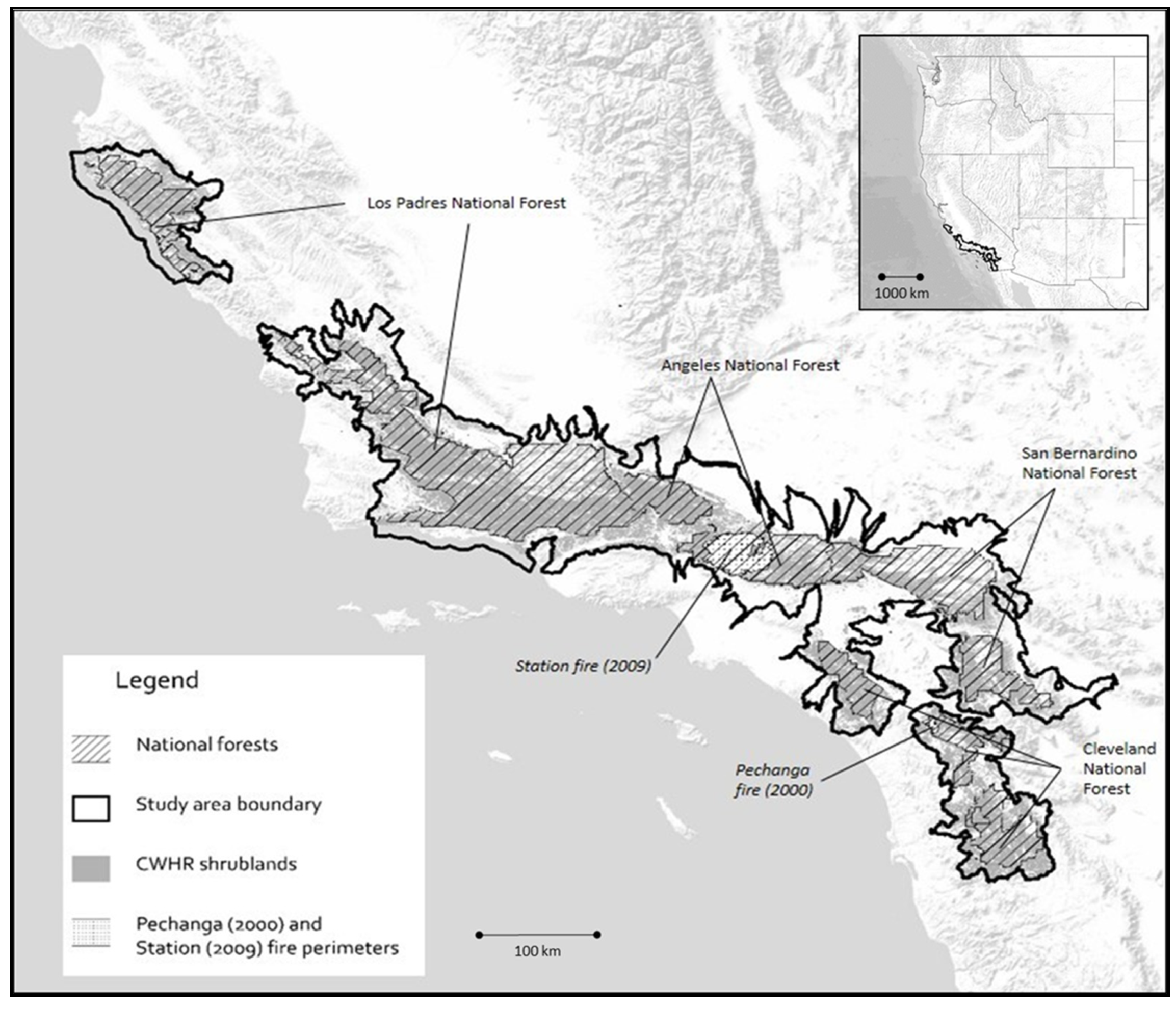
Our study area totaled 3,515,805 ha (8,687,731 acres), defined by all HUC12 (USGS Hydrological Unit Code) watersheds that intersected with USFS National Forests in Southern California (Angeles, Cleveland, Los Padres, and San Bernardino, hereafter ANF, CNF, LPNF, and SBNF, respectively) (Figure 1). The Mediterranean-type climate in the study area is characterized by warm dry summer months and mild wet winters with most of the annual precipitation occurring in the winter and spring. Elevation in the study area ranges from 133 to 2231 m. Shrublands accounted for over half (54%) of the natural vegetation in the study area, followed by conifer and hardwood forest (<20%) in higher elevation areas. Wildfires are a common disturbance [9,14] with an estimated 5580 ha per year of the study area burned (estimated from Reference [36]). Although we focused on the AGLBM of chaparral shrublands, we estimated biomass for all wildland vegetation types in the study area.
2.2. Environmental Data Layers
We assembled environmental data layers considered useful for predicting biomass based on input from USFS resource managers, ecologists, and studies in the literature (e.g., [37]). Given our objective to develop a model that can be applied to different years based on that years’ Landsat NDVI reflectance and precipitation, we divided our predictive variables into two categories: time-dependent and static.
Static predictors included geophysical features of the landscape: aspect, slope, elevation, flow accumulation, partitioning around medoids (PAM), [39], solar radiation, geomorphons, and soils (all at 30 m resolution, see Table 1). We also included the 30 year average of several climatic variables: annual precipitation, climatic water deficit, groundwater recharge, water runoff, and actual evapotranspiration as calculated by the Basin Characterization Model [40].
Time-dependent predictors are specific to the target biomass year being analyzed and included the annual (previous year) and biennial (previous 2 years) total precipitation and NDVI data from Landsat imagery (2000–2019, see Section 2.3). Considering the great importance of precipitation in biomass development post-disturbance [41,42], we selected short-term precipitation predictors (annual and biennial) that mediate shrub leaf development and grass/forb production, while the long-term average precipitation regulates more persistent woody biomass development [43]. For analysis purposes, we established the year as 1 September to 31 August to coincide with the end of the primary growing season and before September and October—a period of historically of extreme wildfires [44].
Annual and biennial precipitation data were obtained from ClimateNA v5.10 software, which compiles precipitation data from the Parameter-Elevation Regressions on Independent Slopes Model (PRISM) [45]. Using the ClimateNA software, we downscaled the monthly PRISM precipitation data from 4 km to 500 m; ClimateNA employs a bilinear interpolation and local elevation adjustment to reduce the scale of gridded climate data [46]. The monthly precipitation raster files were summed for the annual and biennial periods for each year from 2000 to 2019. We prepared all of the environmental data layers so that the pixel size (30 m) and projection matched using R version 3.6.0 with the raster package version 3.0.12 and ArcGIS Pro version 2.5 software.
2.3. Landsat TM Data and Vegetation Indices
We obtained Landsat 5, 7, and 8 surface reflectance (http://landsat.usgs.gov/CDR_LSR.php, accessed on 15 November 2018) maximum value composite images for July and August for each year from 2000 to 2019 from the Google Earth Engine data catalog (https://earthengine.google.com/datasets/, accessed on 14 December 2018) using the JavaScript Application Programming Interface (API) [47]. This code extracted the maximum value for each of the bands and calculated the Normalized Difference Vegetation Index (NDVI) using the following formula:
where nir = near-infrared band (OLI band 5, TM/ETM+ band 4), red = red band (OLI band 4, TM/ETM+ band 3), and blue = blue band (OLI band 2, TM/ETM+ band 1). For the period 2000–2011, we used Landsat 5 TM and Landsat 7 ETM+ data. Landsat 5 TM data have pixel drops/errors, so to reduce the effect of these, we masked and replaced them with Landsat 7 pixels from the same year. In July/Aug 2012, Landsat 8 was not yet operational, and Landsat 5 had stopped collecting data, so for this year, we used Landsat 7. Landsat 7 ETM+ data have artifacts related to the scan line correction failure that occurred in 2008; thus, we limited the use of these data to 2012. For 2013–2019, we used Landsat 8 OLI data.
(nir − red)/(nir + red),
The revisit period for both Landsat 5, 7, and 8 is 16 days, so at most there would be two scenes available for any given month. The maximum NDVI value pixel was extracted from the collection of all NDVI pixels from all available scenes from July and August of each year. This raster product is called the maximum value composite (MVC).
Shrublands in Southern California are influenced by precipitation-driven flushes of herbaceous/grass vegetation, particularly in the winter and spring months [48]. Since our objective was to estimate woody shrub biomass, we minimized the effects of these ephemeral pulses of herbaceous vegetation using July–August MVCs when the herbaceous layer was largely senesced. Assuming that we had, at a minimum, 3 scenes for each compositing period, we were reasonably assured of cloud-free pixels throughout the study area for any given year. A July–August NDVI MVC was created for each year 2002–2019.
2.4. Plot Data for Biomass Estimates
2.4.1. USFS Forest Inventory and Analysis Data
We used 668 plots from the USFS Forest Inventory and Analysis (FIA) program, which is a network of inventory and monitoring plots across the conterminous US. These plots represent a sample of forested lands across all ownerships that provide consistent, scientifically reliable forest inventory data. Visit dates for our plots were distributed between the years 2001, 2002, 2004, 2008, 2010, and 2012. All FIA plots used in this study were located on USFS administered lands.
An FIA plot consists of four circular subplots (radius 7.32 m) with three of the subplots arranged at angles of 360°, 120°, and 240° and 36.6 m from the center subplot. In total, the four subplots sample 673 m2 and can intersect with four to eight 30 m Landsat pixels (depending on the plot center location relative to the pixel grid) [49].
In the FIA data collection procedure, the crown diameter and height of all individual shrubs were recorded on the four subplots within each plot. Using these measurements, we applied species-specific allometric equations [50,51] to calculate the AGLBM of shrub species where possible, otherwise we used a generalized shrub–herb biomass equation [52]:
where B is biomass (kg/m2), H is height (m), C is percent cover/100, and BD is the bulk density (kg/m3) constant of 0.8 for grass and herbaceous plants and 1.8 for shrubs. Biomass was calculated for shrub and herbaceous species with ≥3% cover in the subplot.
B = H × C × BD
To estimate the biomass of trees, we first defined classes using diameter at breast height (dbh) measured 1.37 m above ground level: “trees”, ≥12.7 cm dbh; “saplings”, 2.54–12.7 cm dbh; “seedlings”, <2.54 cm dbh. We applied regional models that estimate live tree AGLBM using the component ratio method; inputs included dbh, height, and species. The AGLBM biomass estimates did not include tree foliage such as needles and leaves. We calculated sapling AGLBM using a modified biomass equation from Reference [53] with an adjustment factor based on sapling dbh [54]. For sapling woodland tree species with multiple stems close to the ground (e.g., Quercus gambelii and Cercocarpus ledifolius), diameter was measured at the root collar [55]. Seedling (<2.54 cm dbh) biomass was not recorded and shrub data were not collected on plots visited after 2010 in the FIA plots. After calculating the biomass for each individual shrub and tree (≥12.7 cm) species, we compiled the total AGLBM density (kg/m2) for the plot in each of the three categories: tree, shrub, and herbaceous.
2.4.2. LANDFIRE Reference Database
The LANDFIRE plot data (LANDFIRE Reference Database (LFRDB)) were collected from a variety of sources to generate and validate the LANDFIRE products, including vegetation, fuel, and fire frequency, that can be used as inputs into fire behavior models (https://www.landfire.gov/, accessed on 13 June 2019). We downloaded approximately 6000 LFRDB records for the Southern California study area collected between 2000 and 2005. Of these 6000 plots, 276 contained the vegetation data (i.e., cover and height) required to calculate biomass and were in our study area. These data were collected in 2005, using the FIREMON protocol (https://www.fs.fed.us/rm/pubs/rmrs_gtr164.pdf, accessed on 6 July 2019), which consists of a series of variable radius and shape subplots all with the same macroplot center. Individual shrub and plant data were not recorded, instead the average cover and height of live vegetation in two height classes (<1.83 m and >1.83 m) were estimated. We estimated AGLBM using the general equation [52] for both height classes. Herbaceous cover and height were also present in LFRDB, so we calculated these as a separate category, again using the generalized biomass equation. The LFRDB plots in the study area had no data on trees, so we assumed that they were not present. To avoid underestimating AGLBM in plots with trees, we confirmed their absence by examining plot locations with the high-resolution imagery contained in Google Earth desktop software (GE) and eliminated any that appeared to have trees. The AGLBM was summed in the three categories (<1.83 m, >1.83 m, and herbaceous) to provide total AGLBM in each plot (kg/m2).
2.4.3. Additional Field Plot Data
We obtained data from two research projects to integrate with the FIA and LFRDB plots [41,56]. Vourlitis (2012) sampled biomass on the same plots quarterly (2004–2016) using non-destructive dimensional analysis as part of a study on the effects of added nitrogen on chaparral productivity. The experimental design used four 10 m × 10 m plots as the untreated control; we used the biomass sampled on these control plots during the summer quarter (July–August–September) for the years 2004–2016. Uyeda et al.’s (2016) study tested growth ring analysis as a proxy for post-fire biomass recovery in chaparral. This study developed species-specific regression equations from a sample of harvested shrubs; these equations related stem basal area to biomass. These equations were then used to estimate biomass on twenty-four 16 m2 plots on the USFS San Dimas Experimental Forest. All stem measurements were conducted in the fall of 2013. In cases where the plots fell in the same Landsat pixel, these plots were averaged, resulting in the elimination of three plots.
Finally, we sampled five plots in June 2019 within the Powerhouse fire which burned in 2013 using a 30 m × 0.5 m belt-transect to collect vegetation height and cover for shrub species. Grass and forb cover were estimated using the point–line intercept method from points sampled every 30 cm along the transect. We used the same allometric equations described above to estimate AGLBM; for species with no allometric equation, we applied the general equation [52].
Our gross number of plots before filtering was 959: 668 FIA, 276 LFRDB, 10 from Vourlitis (2012), and 5 from the Powerhouse fire data collection campaign. Uyeda et al.’s (2016) data were set aside for validation purposes, because their methods estimated field biomass without the use of allometric or general equations and so provided an opportunity for validation independent of estimates determined with these equations. Filtering criteria included removing any FIA plots with zero biomass (e.g., where plots contain only herbaceous cover or several species that individually do not comprise the 3% cover threshold). The FIA plot visits after 2010 did not collect any data on shrubs, forbs, or grasses so these plots were reviewed in GE with historical high-resolution images. If plots were determined to be tree-dominant by ocular estimation, they were retained so we could calculate biomass, otherwise they were removed from the plot database. Our logic here was that if the plots were tree dominant, then the lack of any biomass data for shrubs and forbs would be negligible. We filtered the data for outliers using the 1.5 quartile rule where plots with AGLBM values that were lower than Q1 − 1.5 (Q3 − Q1) and higher than Q3 − 1.5 (Q3 − Q1) (Q1 = the first quartile of the data distribution, and Q3 = the third quartile of the data distribution) were removed from the plot data (1.5 × interquartile range rule, [57]). Further screening was undertaken of suspect plots identified in scatterplots of AGLBM versus the predictor variables and reviewed in Google Earth, which reduced the final number of plots used in the model to 766.
2.4.4. Assigning Predictor Values to Plots
The predictor spatial data were 30 m in resolution, but because of uncertainty in the plot location, the continuous predictor variables (i.e., aet, aspN, aspE, cwd, dem, facc, ppt_1yr, ppt_2yr, ppt_avg, rch, run, solrad, slope, NDVI, see Table 1) were extracted using bilinear interpolation, while the remaining categorical variables (i.e., geomorph, PAM, soils) were extracted with no interpolation. Predictor values were assigned to each plot with a python script that used the ArcGIS Python API tool “Multi-values to points” to extract the values from the predictor raster layers.
We assigned NDVI and annual/biennial precipitation values to the plots based on the calendar year of the field visit. To confirm there had been no change in plot cover since they were measured, we reviewed wildfire perimeter polygons from the CalFire FRAP website (https://frap.fire.ca.gov/frap-projects/fire-perimeters/, accessed on 21 March 2020) for each plot. Plots that experienced a disturbance after the field visit were analyzed in Google Earth to assess if substantial vegetation changes had occurred before the NDVI data were acquired, if yes, then the plots were omitted.
Finally, we randomly split our dataset into training (614 plots) and validation (152 plots), excluding the validation plots in building the biomass model (Table 2).
Reserving an independent set of validation data enabled us to analyze errors by vegetation class and to compare our model results to AGLBM estimates from other sources using the same dataset.
2.5. Estimating AGLBM with Random Forest
To build a predictive regression model to estimate AGLBM from the FIA, LFRDB, and other field data, we used random forest (RF, randomForest package version 4.6.14 in R software), an ensemble machine learning algorithm. RF builds a “forest” of decision trees; each tree is built using a random selection of predictors and samples from the training data. Random forest has two parameters that are used to optimize the computed regression model—mTry, the number of predictors used in each regression tree and Ntree, and the number of regression trees grown. During the training stage, RF withholds a random sample of 1/3 of the plots (out-of-bag samples or OOB) for cross-validation, while the remaining two-thirds are used to build the regression tree [58]. We repetitively ran RF with different combinations of mTry and Ntree to maximize accuracy (high percent variance explained, low OOB RMSE).
By randomly shuffling the values of a predictor variable while preserving the values of all other variables during OOB validation, the relative importance of the variable in the model is calculated. The importance is expressed as the percent increase in mean standard error if the variable is excluded from the model. This is called variable importance. Random forest is relatively insensitive to multicollinearity issues arising from the inclusion of highly correlated variables [58]; nevertheless, we built a correlation matrix of the predictor variables during our data exploration.
After creating the optimized model, we wrote an R script [59] that ingested the predictor layers (Table 1), including the time-dependent NDVI and precipitation layers matched to the target year, to build a continuous AGLBM surface raster for each target year from 2000–2019. Before running the script, we masked out urban, water, and agriculture land cover from the predictor layers using the California Wildlife Habitat Relations (CWHR) “WHR Type” classification [38]. Hereafter, we refer to our AGLBM estimates as the WETAC-UCD estimates. Following inspection of the WETAC-UCD raster layers, we determined that the predicted biomass of perennial grassland and desert scrub CWHR classes [38] was higher than field based estimates [60,61] by approximately 2 orders of magnitude, so we reduced AGLBM values for these classes by 99% and 90%, respectively. All estimates of biomass are provided in kg/m2.
We assessed the accuracy of the final RF model in several ways. First, each of the OOB samples (one-third of the plots) was run through the RF tree to report the variance and associated mean of squared residuals and mean standard error (MSE). This was done as a part of the RF process. Second, using the 20% validation data (168 plots) we reserved prior to running the RF model, we conducted a k-fold cross-validation of the model predictions. This method splits validation data into k subsets, reserves one subset and runs the model with the remaining k-1 subsets, and calculates the average prediction error rate. Next, we generated linear regression models of actual versus predicted AGLBM by cross-referencing the validation data with the CWHR vegetation class to create linear models for each vegetation class that constituted 1% or more of the USFS lands in the study area. To overcome the insufficient number of plots in some classes, we also compared modeled and actual estimates for aggregated groups (all shrub, all needle-leaf, and all hardwood) and finally all CWHR classes. Finally, we created linear regressions with the Uyeda et al. (2016) data, which used field-based biomass measurements rather than allometric equations, to test for bias in the methods used to calculate AGLBM from the FIA and LFRDB data.
2.6. Comparison of WETAC-UCD Estimates with Other Global and Statewide Biomass Datasets
To view our AGLBM estimates in a broader context and to provide useful information for resource managers, we compared our 2010 WETAC-UCD data to two contemporary spatial biomass estimates for the four southern USFS national forests: the Global Harmonized Carbon Density Data for the year 2010 (GHCD at 300 m resolution) [60], and the statewide California Air Resources Board (ARB at 30 m resolution) carbon stocks for 2010 [61,62]. We converted the raster biomass data from these projects to kg/m2 of biomass (rather than carbon) to compare with our WETAC-UCD AGLBM estimates. In addition, the GHCD data were resampled from the original 300 m pixel size to 30 m to match the resolution of the WETAC-UCD data.
We compared our estimates to the GHCD and ARB biomass estimates in two ways: (1) We isolated pixels by creating three different groups and created corresponding raster masks from the CWHR vegetation data to permit comparison: shrubland (mixed chaparral, chamise-redshank chaparral, coastal scrub, montane chaparral, and sagebrush); non-shrubland (montane hardwood, pinyon-juniper, Sierran mixed-conifer, coastal oak woodland, montane chaparral Jeffery pine, annual grassland, and eastside pine); finally, all vegetation pixels (both shrub and non-shrub types listed above). Next, we calculated mean biomass in these three categories for each of the three estimates for each national forest in the study area. We tested for differences between the AGLBM means for shrub types, non- shrub types, and all CWHR vegetation types that were 1% or more of the USFS lands in the study area for each national forest using the two-sample t-test. (2) We extracted the 2010 biomass values from each of the three sources for all validation plots visited in 2010 and built linear models to examine the relationship between the field and modeled biomass estimates.
2.7. Comparison of WETAC-UCD Estimates with Field Estimated Biomass
In addition to comparisons made with the remote sensing-based datasets described above, we also wanted to compare the WETAC-UCD AGLBM estimates to field estimates published in the literature. To do this we cross-referenced our estimates with biomass estimates compiled by Bohlman et al. (2018) [17], hereafter referred to as Bohlman, based on a literature review of 37 research studies spanning 72 years in California shrublands. The review summarizes field studies by three CWHR shrubland classes—mixed chaparral, chamise-redshank chaparral, and coastal sage scrub—and age class (i.e, time since fire disturbance). Using stand age and CWHR vegetation type, Bohlman calculated the average biomass increment (kg/m2/year) by age class. The age class breaks varied by vegetation type (reflecting the available data): mixed chaparral, 1–10 y, 11–20 y, and 21–30 y; chamise chaparral, 1–10 y, 11–30 y, and >30 y; coastal scrub, 1–10 y and >10 y. To compare, we generated data for the three shrubland types and two age classes (1–10 years, 11–20 years) from within the perimeters of the Station fire (2009) located on the Angeles National Forest and the Pechanga fire (2000) on the Cleveland National Forest. Note, no comparison can be made with Bohlman’s 21–30+ age class, because the oldest fire analyzed (Pechanga) was only 20 years post-fire.
We focused on biomass data from the Station and Pechanga fires as they had at least 10 years of post-fire recovery, contained adequate amounts of all three vegetation classes, were not substantially impacted by multiple fires during 1980–2019, and both burned at the same time of year (late July–August). Fire history data were obtained from the Fire Return Interval Database (FRID) compiled annually by the USDA Forest Service [15] and fire perimeter data from the CalFire FRAP website (https://frap.fire.ca.gov/frap-projects/fire-perimeters/, accessed on 21 March 2020). A series of spatial raster masks were developed for each CWHR type, first to mask pixels within these fires that only burned once in 1980–2020 and, second, to identify pixels that burned at a high intensity (using data from the USDA Forest Service Rapid Assessment of Vegetation Condition after Wildfire (RAVG) program [63]). Masks were applied to each of the annual AGLBM raster layers and statistics calculated, producing a table of 2000–2019 AGLBM for both fires.
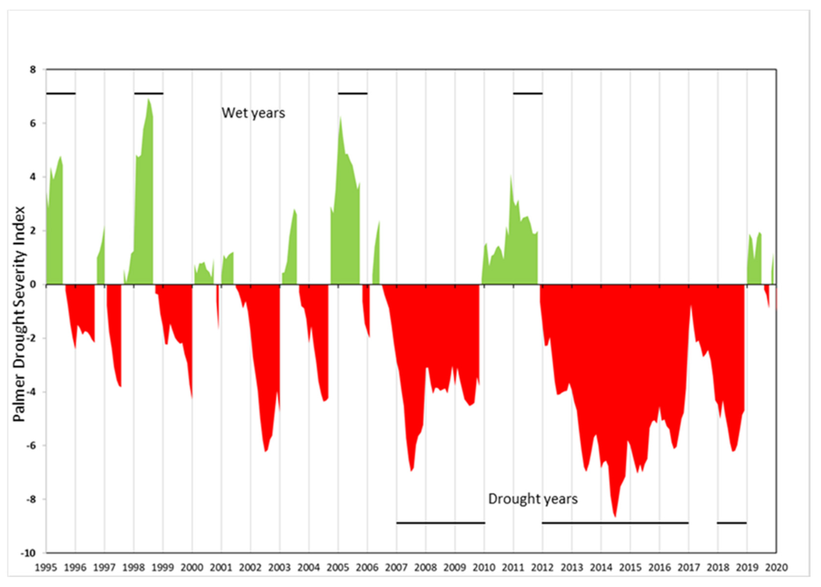
We also focused on biomass estimates from “normal” precipitation years by excluding abnormally dry and wet years to avoid any bias related to precipitation from our recovery estimates. Abnormally wet and dry years were determined using the Palmer Drought Severity Index (PDSI) [64]. The PDSI is determined on a 2.5 degree by 2.5 degree grid and compiled monthly for the National Climate Data Center’s US Climate Division (https://www.ncdc.noaa.gov/monitoring-references/maps/us-climate-divisions.php accessed 4/18/2020). The range of these data is 10 (very wet) to –10 (very dry). We used PDSI data from the South Coast Drainage division boundary which corresponded closely with our study area boundary. Monthly South Coast Division PDSI values were assembled in a data table for the years 1995–2020. We defined a drought year as containing 4 or more consecutive months with a PDSI of less than –3 (severe or extreme) in the growing season (November to May) and a wet year as 4 or more consecutive months with a PDSI of 2 or greater (moderately moist to very moist) in the same period (Appendix A).
3. Results
3.1. Estimating AGLBM with Random Forest
3.1.1. Plot Data
Out of a 152 variable pairs, eight were highly correlated (R2 > 0.50). Six of these pairs were hydrological or precipitation variables and the remaining two were solrad–aspE and cwd–aet (see Table 1). Given the low number of highly correlated variables and the ability of RF to handle multicollinearity issues without bias, we opted for retaining all predictors.
Using the biomass calculations from the species-specific and general equations, the 627 plots used in the RF model (hereafter referred to as the RF plots) ranged in total AGLBM from 0.02 to over 46 kg/m2. All RF plots over 16 kg/m2 AGLBM were in forested CWHR types including pinyon-juniper, montane hardwood, and coastal oak woodland. The allocation of RF plots by CWHR types (accounting for >5% of the study area) included: 270 plots in mixed chaparral (32% of the study area), 62 in pinyon-juniper (3% of the study area), 48 in chamise-redshank chaparral (6% of the study area), 45 in montane hardwood (3% of study area), 32 in coastal scrub (8% of the study area), and 35 in coastal oak woodland (5% of the study area).
3.1.2. RF Model
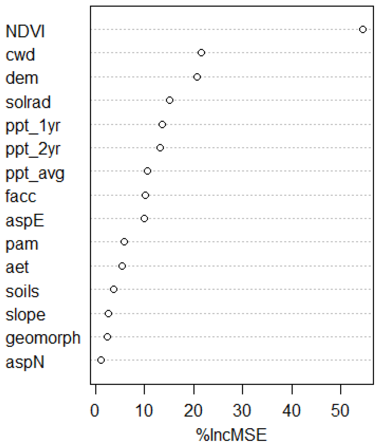
Our final RF model (mTry = 8, Ntree = 1000) explained 49% of the variance in the OOB samples, with an accompanying RMSE of 4.0. The k-fold cross validation R2 was 0.51 and had an RMSE of 3.9. The NDVI was definitively the most important variable in our model (Figure 2)—over twice that of the next ranking variable. A second tier of variables included cwd and DEM, followed by solar radiation and annual and biennial precipitation. Together they would account for an increase in MSE of 46% if removed from the model.
3.2. Validation by CWHR Vegetation Class
The statistics for the linear regression models of the validation plots for each CWHR class ranged from R2 = 0.51 (Pinyon-Juniper, RMSE = 1.5) to 0.23 (Mixed chaparral, RMSE = 2.4) (Table 3). Many of the CWHR classes contained less than 10 validation plots and their regression models were not significant at the 5% level. Table 3 presents the regression metrics for all vegetation types that comprised 5% or more of Forest Service lands in the study area. Aggregating the CWHR types into shrub, needle-leaf, and hardwood super-classes revealed that shrub types had a weak to moderate significant relationship with the field validation plots (R2 = 0.30, RMSE = 2.3 (138% of mean)), while the needle-leaf and hardwood types were moderate to strong (R2 = 0.53, RMSE = 3.9 (83% of mean) and R2 = 0.49, RMSE = 7 (89 % of mean), respectively). The model that included all CWHR types was also moderate to strong (R2 = 0.54, RMSE = 3.8 (112% of mean)), like the k-fold cross-validation values from the RF model.
3.3. Comparison of WETAC-UCD Estimates with Other Global and Statewide Biomass Datasets
To evaluate our WETAC-UCD data with global and statewide biomass estimates and provide useful information for resource managers, we compared the GHCD (global) and ARB (California) biomass estimates for the four Southern Californian national forests for 2010. These national forests (NFs) have distinct geographies, vegetation types, and fire histories that are evident in their respective biomass estimates (Table 4). The LPNF is the most northerly of the national forests and contains coastal forests, resulting in more productive vegetation types. Consequently, it has the highest mean WETAC-UCD AGLBM in all three vegetation categories (shrub only, non-shrub only, and all vegetation types). The drier, most southerly forest, CNF, had the lowest mean WETAC-UCD AGLBM for all three classes.
On each NF (by shrub, non-shrub, and all vegetation classes), the GHCD AGLBM (with one exception) and ARB estimates (except for the LPNF) were consistently higher than the WETAC-UCD estimates.
Mean delta values between the WETAC-UCD estimates and the ARB estimates for all four NFs were comparable: 0.25 kg/m2 for shrub vegetation and 0.45 kg/m2 for non-shrub vegetation. In contrast the GHCD–WETAC-UCD delta values were much higher (2.3 kg/m2) for shrub vegetation than non-shrub (0.78 kg/m2).
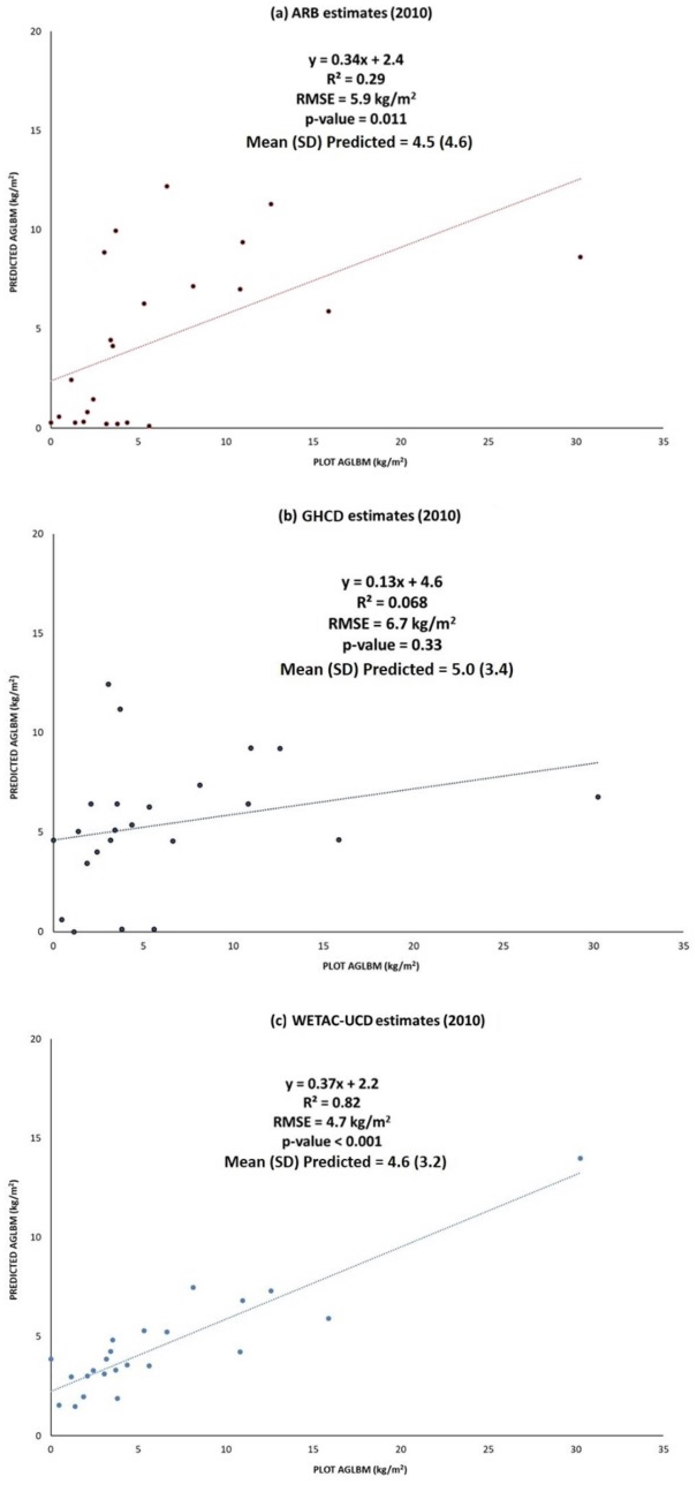
Linear models using the 22 validation plots sampled in the year 2010 for the WETAC-UCD, ARB, and ORNL-UCD estimates indicate the WETAC-UCD data best predicted the field AGLBM estimates (R2 = 0.82, RMSE = 4.7 kg/m2) (Figure 3), followed by the ARB model (R2 = 0.29, RMSE = 5.9 kg/m2). Mean biomass values for these plots were not significantly different for all three estimates at the 1% level. The model for the GHCD and WETAC-UCD data was not significant at the 5% level (p-value = 0.33). RMSE values for all three models were high (6.7–4.7 kg/m2) compared to the mean biomass values presented in Table 3.
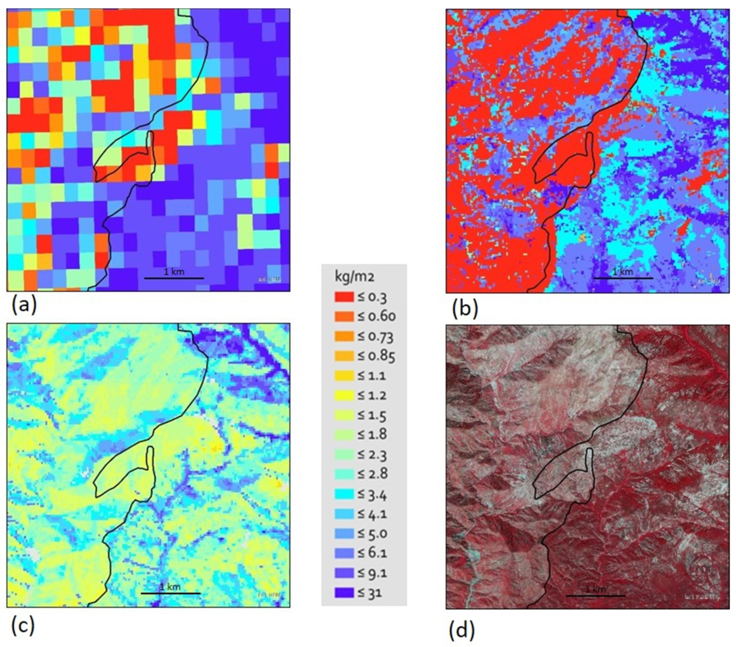
Finally, we compared maps of the WETAC-UCD (30 m), GHCD (300 m), and ARB (30 m) data for 2010 using a mixed-chaparral-dominated area on the ANF that contained part of the Station fire (September 2009) (Figure 4). Two things were notable: First, the WETAC-UCD data showed more discrimination in AGLBM values of vegetation associated with landscape features than the coarser scale GHCD data. Second, the WETAC-UCD did not reflect the Station fire footprint as prominently as the other two sources of data, i.e., there were no pixels with the very low levels of biomass (Figure 4c). The effects of the Station fire on AGLBM were not prominent in our data because nearly a year of regrowth had occurred in the image (Figure 4c) given the timeframe used in our methods. Many shrub species have resprouting post-fire life histories and so can resprout vigorously with rapid growth post-fire, consequently, there can be considerable biomass within one-year post-fire. Our approach utilized data from July–August (2010) to capitalize on capturing AGLBM of shrubs versus herbaceous vegetation, compared to the unknown month of calculation for the GHCD (Figure 4a) and the ARB (Figure 4b) images.
3.4. Comparison of WETAC-UCD Estimates with Field Measured Biomass
Compared to Bohlman, our estimates were consistently higher for all shrub types and age classes (Table 5). Bohlman’s average annual biomass increment estimates were higher for all shrub vegetation age classes, with the exception of the 11–20 year chamise chaparral class where no data from the literature review were available. Early post-fire recovery (1–10 years) was higher for the WETAC-UCD estimates, but for the 11+ year age classes, AGLBM values for the two estimates were much closer.
4. Discussion
In this study, we present a repeatable and transparent biomass model that is a substantial improvement in accuracy over two other estimates that include shrublands at both statewide and global scales (Figure 3). In addition, by adjusting the time-dependent predictors in our model, it can be applied consistently across different years, yielding a temporal stack of biomass estimates that can be used to assess recovery after disturbance. Our estimates by age class and vegetation type are generally consistent with field estimates from the literature [17] (Table 5), particularly among the older (>10 years) age classes.
The foundation of this work has been the inclusion of shrub measurements into FIA plot re-visits for 2001–2010 on the four Southern California NFs, which provided essential data. However, there are two potential issues with the plot data that we used. First, accurate plot locations are essential so that the correct raster values can be associated with the plot measurements. However, little information was available on the methodology or accuracy of the FIA or LFRDB plot geolocations, which raises questions as to whether the value of the pixel at plot center correctly represents the plot. Second, given that making in situ biomass measurements is time-consuming and costly, typically involving destructive sampling of vegetation, separation of components (i.e., stems, leaves, roots), followed by drying and weighing of these separate materials [66], we used allometric equations to estimate biomass from the FIA and LFRDB plots. Both the allometric equations and especially the general equation undoubtedly are sources of error in estimating the true quantity of biomass at the plot level. We used species-specific allometric equations for 14 shrub species and two genera from two studies [50,51]; for the remaining shrub species with no published allometric equation, we used a general equation (described in Section 2). This equation uses a generic bulk density constant for all shrubs and is a general approximation that is probably relatively low for many species [67,68,69]. Biomass estimates using the general equation have a moderate to strong relationship with allometric equation estimates (Appendix B), but further work is necessary to examine the accuracy of these estimates to in situ data on chaparral shrub species. In addition, the bulk density constant used for forbs and grasses has also been shown to yield underestimates of grass biomass [70].
To maintain consistency, we used the same suite of allometric equations on the Powerhouse plots as the FIA data; the LFRDB data used the general equation and Uyeda et al. (2016) used AGLBM calculation methods that did not use these equations. Many of the equations used were developed outside of Southern California. Further work is needed to develop and refine allometric models and bulk density constants for chaparral species. Finally, the FIA methods did not specify recording tree seedlings or any shrub or forb with <3% cover; presumably, if seedlings were present in significant number or if there were several species present with less than 3% cover, this could also result in an underestimation of plot biomass.
The NDVI is a proven spectral index in assessing vegetation in Mediterranean-type shrublands [32,42,48,71]. In our RF model, it ranks highest in variable importance (Figure 2). This is an important consideration as NDVI, along with annual and biennial precipitation are the time-dependent predictors—the factors that are defining the year-to-year changes in biomass. Chaparral landscapes in Southern California are subject to highly variable precipitation, and AGLBM varies accordingly. This is also reflected in the variable importance of our model; annual and biennial precipitation (ppt_1yr and ppt_2yr, respectively) are the 5th and 6th most important variables in the model. The importance of climatic water deficit in our model confirms the findings from other studies in California’s shrublands [72] and shows that the availability of soil moisture and not just precipitation is a critical factor in the production in drought-prone chaparral communities. Short-term fluctuations in precipitation probably influence AGLBM through corresponding fluctuations in leaf area and herbaceous/grass production, while soil moisture is an indication of a site’s ability to support perennial woody vegetation.
There was consistency in the validation statistics for the model (k-fold cross validation R2 = 0.51, OOB RMSE = 4.0) and from the validation plot metrics (R2 = 0.54, RMSE = 3.8 for all CWHR types), suggesting that our model is capable of making good predictions for observations not used to build the model.
Although our focus was on improving AGLBM estimates for chaparral shrublands, we did include all wildland vegetation types in this study. Breaking down our AGLBM estimates by CWHR class allowed us to explore errors or inaccuracy that might be associated with vegetation type, although for many of the classes there were few validation plots. The high RMSE values we report for the shrubland CWHR classes are an indication of the spatial heterogeneity in shrubland ecosystems and the difficulty inherent in building a model that captures this diversity accurately at the landscape scale [73]. Furthermore, within a single CWHR vegetation class there may be a wide range of species assemblages and structure types. Ideally, we would have enough field plots for modeling and validation of vegetation classes at a much finer spatial scale. Our model underestimated AGLBM of the validation plots (slope values < 1) for all the CWHR types that were 5% or more of the study area (Table 3). This underestimation is probably increased if we consider the application of the general allometric equation used to calculate AGLBM for most shrub species in the FIA plots and in all the LFRDB plots, which are likely underestimating quantitative field measurements of biomass.
4.1. Comparison of WETAC-UCD Estimates with Other Global and Statewide Biomass Datasets
Since the majority of AGLBM for the continental US is contained in forests and woodlands, it is not surprising that most national and global scale biomass estimates do not address shrublands (see References [21,22]). In these datasets, the total carbon present as well as sequestration capability of chaparral shrublands is low compared to forests. However, this is changing as regions and countries that contain substantial areas of Mediterranean-type shrublands and woodlands are assessing carbon stocks to fulfill agreements under the Kyoto Protocol and the REDD+ (Reducing Emissions from Deforestation and Forest Degradation) project.
We compared our estimates to two previous efforts that also mapped AGLBM for shrublands in Southern California. The goal of the ARB project was to consistently map carbon stocks across California. They assigned AGLBM to LANDFIRE vegetation existing vegetation types (EVT), cover (EVC), and when available existing height classes [62]. This approach, known as “stratify and multiply”, tends to obscure the wide range of AGLBM variability within a vegetation class, which can be observed in Figure 4, and also is subject to inaccuracies in the vegetation classification [62,74]. In our case, the ARB aggregation of AGLBM by LANDFIRE classes resulted in their estimates by forest to be higher than ours (Table 4). Second, the GHCD project goal was to develop a global biomass dataset that captured the uncertainty surrounding both the above and below ground biomass estimates [60]. In developing their datasets, they leveraged the GlobBiomass project [75] for forested areas. Estimates for shrublands and savannahs were developed for Africa using synthetic aperture radar (SAR) [76]. These shrubland/savannah estimates were subsequently applied globally.
We made the comparison between the ARB, GHCD and WETAC-UCD to show that scale matters—compiling statewide and global estimates at the local scale of National Forests obscures the spatio-temporal heterogeneity that is intrinsic to chaparral shrublands (Figure 4). Additionally, it highlights the inaccuracy of shrubland biomass data in these broader scale efforts. However, it is interesting that the means of predicted AGLBM for the 22 validation plots were not significantly different for all three estimates (ARB, GHCD, and WETAC-UCD), suggesting that these estimation methods produce similar values when aggregated, but this does not hold true at the National Forest level. Note, however, that the ARB and GHCD studies place cautionary notes in regard to their shrubland estimates; stating that carbon in shrublands is poorly quantified [61] and that the estimates for shrublands in Spawn and Gibbs (2020) [60] outside of Africa and the arctic used GlobBiomass [75] and did not explicitly estimate shrubland biomass.
Further considerations when reviewing estimates of AGLBM at the NF level is the fire history of each NF which should be reflected in the 2010 AGBLM estimates (presented in Table 4). The LPNF had the highest area burned (41%) between 2005 and 2010. Based solely on this fire history, we would assume that AGLBM would be lower on the LPNF because a greater percentage of the area was in an earlier post-fire successional stage, but that is not the case, meaning that other factors such as greater productivity in more northerly latitudes, location in the coast range, and shrub species with different life histories (e.g., resprouting versus seeding) are involved. However, the effect of fire is evident between the ANF and SBNF; WETAC-UCD AGLBM is lower for the ANF (31% burned) than the SBNF (8% burned).
4.2. Comparison of WETAC-UCD Estimates with Field Estimates
Although most of the AGLBM age class/vegetation type means reported by Bohlman are represented by two or fewer studies, our results are nevertheless comparable (Table 5). The 1–10 year age classes exhibited the biggest differences; one explanation for this is that most post-fire recovery in chaparral communities takes place during this period. Our estimates are the mean of all pixels 1–10 years post-fire (from the Station and Pechanga fires), so there is probably a higher frequency of high AGLBM values than in the Bohlman studies, which are based on temporally and spatially limited field plots. For all vegetation classes except coastal sage scrub, our AGLBM values for years 11–20 were much closer (0.1–0.4 kg/m2 difference) to the values presented in Bohlman. The established vegetation characteristic of these older age classes is more resistant to short-term climatic fluctuations, i.e., AGLBM tends to be more stable compared to the 1–10 year age class where the AGLBM is more sensitive to climatic variation. Future research into post-fire recovery by community type using the WETAC-UCD AGLBM data stack could examine spatial and temporal variations in AGLBM by age class; this may provide further evidence of this trend. Another possible explanation is that our estimates did not include wet or drought years. Over half (60%) of the studies reviewed in Bohlman were conducted in the 1970s and 1980s and no information is provided on which studies occurred in drought or wet years. Assuming that droughts were more prevalent than wet years, we can surmise that the Bohlman’s estimates are relatively low because some were sampled in drought years. Prolonged ecological drought can result in substantial mortality in chaparral shrub species, suppressing AGLBM [11].
Despite the sources of error described above, we have confidence in our AGLBM estimates because of the strong relationship (R2 = 0.69, RMSE = 1.02) they had with the field measurements of AGLBM conducted by Uyeda et al. (2016). This suggests our estimates are better at characterizing AGLBM than the validation statistics (Table 3) indicate, and that there is error in the allometric and general equations used for most of our plot data. Uyeda et al. (2016) used stem growth rings to estimate basal area and biomass [41]. Although limited in geographic scope, the Uyeda et al. (2016) plots were in the mixed chaparral vegetation type which comprised over 50% of our study area. Generating additional species specific allometric equations and refining the bulk density constants used in the general equations would be a valuable contribution for future biomass mapping efforts.
The advantages of adding active remote sensing data (e.g., lidar, radar) to optical data sources is well documented [77,78,79,80]; these data provide vegetation structure that is difficult to extract from optical data alone. Future shrubland mapping efforts should investigate synthetic aperture radar (SAR) and spaceborne lidar (ICESat-2 ATLAS) data in combination with optical data [77,81,82].
5. Conclusions
Mediterranean-type shrublands and woodlands, already noted for their globally important biodiversity [83], are increasingly being recognized for their importance regionally and globally in carbon sequestration [4,29], net primary productivity [29,84,85], and water quantity and quality [86]. Carbon sequestration rates may be comparable to those estimated for temperate old-growth forests [4]. Vegetation biomass is an essential part of the landscape assessment process for these services and the ability of chaparral shrublands to deliver these services is not consistent across spatio-temporal gradients due to the environmental differences (e.g., slope, aspect, and elevation) and disturbance from fire. The USFS mandate to monitor ecosystem services and the impacts on those services due to the fire has led to the development of tools such as SoCal EcoServe, a web-based application that delivers spatial and tabular data on pre- and post-fire ecosystem services in Southern California [87]. The AGLBM data developed in this study are incorporated in the SoCal EcoServe tool.
In this study, we created a transparent and repeatable model that can be used to estimate AGLBM on shrubland dominated landscapes that can be consistently applied annually across the Landsat period of record. This is timely given that the USDA Forest Service is now required to monitor and report on carbon stocks; every National Forest System unit is required to report annually on their efforts to incorporate carbon information in land management plans, projects, decisions, and communications [88]. A principal goal of the WETAC-UCD methodology was to develop an approach that could be applied to different years to assess future inquiries into post-fire recovery of biomass and vegetation type conversion. We accomplished this by using the NDVI and precipitation data specific to the year of the AGLBM assessment. Consequently, it overcomes one of the major limitations of most landscape scale biomass estimates: that they are limited to a single point in time. This is especially important considering the disturbance frequency of chaparral communities.
Given that chaparral shrublands are difficult environments for field work—mature stands are nearly impenetrable, and in Southern California, access is difficult and costly. The AGLBM data we present here are a substantial improvement over the existing statewide and global estimates for shrubland dominated landscapes. As such, they present a valuable step forward in accurately accounting for the role these under-studied communities play in carbon budgets and ecosystem services.
Author Contributions
Conceptualization, C.C.S.-P. and E.C.U.; methodology, C.C.S.-P.; software, C.C.S.-P.; validation, C.C.S.-P.; formal analysis, C.C.S.-P. and E.C.U.; investigation, C.C.S.-P. and E.C.U.; resources, C.C.S.-P. and E.C.U.; data curation, C.C.S.-P.; writing—original draft preparation, C.C.S.-P.; writing—review and editing, C.C.S.-P. and E.C.U.; visualization, C.C.S.-P.; supervision, E.C.U.; project administration, E.C.U.; funding acquisition, E.C.U. All authors have read and agreed to the published version of the manuscript.
Funding
Funding for this study was provided by the USFS Western Wildlands Environmental Threat Assessment Center, USDA Forest Service Pacific Southwest Region, CalFire, and the National Fish and Wildlife Foundation’s Wildfires Restoration Grant Program.
Data Availability Statement
The data presented in this study are available on request from the corresponding author.
Acknowledgments
We would like to thank the following people who provided valuable input throughout the study: Hugh Safford, Nicole Molinari, and Allan Hollander. Special acknowledgement to Nicole Molinari who provided us with a thoughtful and constructive review. We also acknowledge valuable data provided by John Battles, Kellie Uyeda, George Vourlitis, and John Chase and thank Kama Kennedy for her help in FIA data interpretation and processing.
Conflicts of Interest
The authors declare no conflict of interest.
Appendix A
Figure A1.
Palmer Drought Severity Index (PDSI) monthly values for 1995–2020 for the South Coast Drainage US Climate Division in Southern California. Anomalous years (wet or drought) are indicated by the horizontal lines in the upper and lower areas of the graph. Drought years were defined as containing 4 or more consecutive months with a PDSI of less than −3 (severe or extreme) in the growing season (November to May) and a wet year as having 4 or more consecutive months with a PDSI of 2 or greater (moderately moist to very moist) in the same period.

Appendix B

Table A1.
Linear regression model statistics for biomass estimates using species-specific allometric equations and estimates using the general biomass equation [52]. Individual shrub measurements used in these estimates were collected during a field campaign on the Los Padres National Forest in 2020.
| Shrub Species | R2 | SE | Slope | Intercept | p-Value | N |
|---|---|---|---|---|---|---|
| Adenostoma fasciculatum | 0.63 | 0.02 | 1.2 | 0.053 | <0.001 | 380 |
| Arctostaphylos glandulosa | 0.49 | 0.012 | 0.39 | 0.056 | <0.001 | 223 |
| Eriogonum fasciculatum | 0.66 | 0.0020 | 0.24 | 0.0037 | <0.001 | 24 |
| Quercus berberidifolia | 0.52 | 0.13 | 2.6 | 0.17 | <0.001 | 42 |
| Ribes spp. | 0.95 | 0.0077 | 0.68 | 0.018 | <0.001 | 10 |
References
- Rundel, P. California chaparral and its global significance. In Valuing Chaparral; Underwood, E.C., Safford, H.D., Molinari, N.A., Keeley, J.E., Eds.; Springer Series on Environmental Management; Springer International Publishing: Cham, Switzerland, 2018; pp. 1–27. ISBN 978-3-319-68302-7. [Google Scholar]
- Jennings, M.K. Faunal diversity in chaparral ecosystems. In Valuing Chaparral; Underwood, E.C., Safford, H.D., Molinari, N.A., Keeley, J.E., Eds.; Springer Series on Environmental Management; Springer International Publishing: Cham, Switzerland, 2018; pp. 53–77. ISBN 978-3-319-68302-7. [Google Scholar]
- Underwood, E.C.; Safford, H.D.; Molinari, N.A.; Keeley, J.E. Valuing Chaparral: Ecological, Socio-Economic, and Management Perspectives; Springer International Publishing: Cham, Switzerland, 2018; ISBN 978-3-319-68303-4. [Google Scholar]
- Jenerette, D.; Park, I.; Andrews, H.; Eberwein, J. Biogeochemical cycling of carbon and Nitrogen in chaparral dominated ecosystems. In Valuing Chaparral; Underwood, E.C., Safford, H.D., Molinari, N.A., Keeley, J.E., Eds.; Springer Series on Environmental Management; Springer International Publishing: Cham, Switzerland, 2018; pp. 141–169. ISBN 978-3-319-68302-7. [Google Scholar]
- Luo, Y. Terrestrial Carbon–Cycle Feedback to Climate Warming. Annu. Rev. Ecol. Evol. Syst. 2007, 38, 683–712. [Google Scholar] [CrossRef] [Green Version]
- Keeley, J.E.; Davis, F.W. Chaparral. In Terrestrial Vegetation of California, 3rd ed.; University of California Press: Oakland, CA, USA, 2007; pp. 339–366. ISBN 978-0-520-24955-4. [Google Scholar]
- Riggan, P.J.; Goode, S.; Jacks, P.M.; Lockwood, R.N. Interaction of Fire and Community Development in Chaparral of Southern California. Ecol. Monogr. 1988, 58, 155–176. [Google Scholar] [CrossRef]
- Keeley, J.E.; Syphard, A.E. Climate Change and Future Fire Regimes: Examples from California. Geosciences 2016, 6, 37. [Google Scholar] [CrossRef] [Green Version]
- Safford, H.D. Man and Fire in Southern California: Doing the Math. Fremontia 2007, 35, 25–29. [Google Scholar]
- Safford, H.D.; Van de Water, K.M. Using Fire Return Interval Departure (FRID) Analysis to Map Spatial and Temporal Changes in Fire Frequency on National Forest Lands in California; USDA Forest Service, Pacific Southwest Research Station: Albany, CA, USA, 2014. [Google Scholar]
- Jacobsen, A.L.; Pratt, R.B. Extensive Drought-associated Plant Mortality as an Agent of Type-conversion in Chaparral Shrublands. New Phytol. 2018, 7, 498–504. [Google Scholar] [CrossRef] [PubMed] [Green Version]
- Harmon, M.E.; Marks, B. Effects of Silvicultural Practices on Carbon Stores in Douglas-Fir Western Hemlock Forests in the Pacific Northwest, U.S.A.: Results from a Simulation Model. Can. J. For. Res. 2002, 32, 863–877. [Google Scholar] [CrossRef] [Green Version]
- Ryan, M.G.; Harmon, M.E.; Birdsey, R.A.; Giardina, C.P.; Heath, L.S.; Houghton, R.A.; Jackson, R.B.; McKinley, D.C.; Morrison, J.F.; Murray, B.C.; et al. A Synthesis of the Science on Forests and Carbon for U.S. Forests; Issues in Ecology; Ecological Society of America: Washington, DC, USA, 2010; pp. 1–16. [Google Scholar]
- Keeley, J.E.; Safford, H.D. Fire as an ecosystem process: Chapter 3. In Ecosystems of California; Mooney, H.A., Zavaleta, E.S., Eds.; University of California Press: Oakland, CA, USA, 2016. [Google Scholar]
- Van de Water, K.M.; Safford, H.D. A Summary of Fire Frequency Estimates for California Vegetation before Euro-American Settlement. Fire Ecol. 2011, 7, 26–58. [Google Scholar] [CrossRef]
- Black, C.H. Biomass, nitrogen, and phosphorus accumulation over a southern California fire cycle chronosequence. In Plant Response to Stress. NATO ASI Series; Tenhunen, J.D., Catarino, F.M., Lange, O.L., Oechel, W.C., Eds.; SeriesG: Ecological Sciences; Springer: Berlin/Heidelberg, Germany, 1987; Volume 15. [Google Scholar]
- Bohlman, G.N.; Underwood, E.C.; Safford, H.D. Estimating Biomass in California’s Chaparral and Coastal Sage Scrub Shrublands. Madroño 2018, 65, 28–46. [Google Scholar] [CrossRef]
- Allen, E.B.; Williams, K.; Beyers, J.L.; Phillips, M.; Ma, S.; D’Antonio, C.M. Chaparral Restoration. In Valuing Chaparral: Ecological, Socio-Economic, and Management Perspectives; Underwood, E.C., Safford, H.D., Molinari, N.A., Keeley, J.E., Eds.; Springer International Publishing: Cham, Switzerland, 2018; pp. 347–384. ISBN 978-3-319-68303-4. [Google Scholar]
- Pratt, R.B.; Jacobsen, A.L.; Ramirez, A.R.; Helms, A.M.; Traugh, C.A.; Tobin, M.F.; Heffner, M.S.; Davis, S.D. Mortality of Resprouting Chaparral Shrubs after a Fire and during a Record Drought: Physiological Mechanisms and Demographic Consequences. Glob. Chang. Biol. 2014, 20, 893–907. [Google Scholar] [CrossRef] [PubMed]
- Syphard, A.D.; Brennan, T.J.; Keeley, J.E. Extent and Drivers of Vegetation Type Conversion in Southern California Chaparral. Ecosphere 2019, 10, e02796. [Google Scholar] [CrossRef]
- Blackard, J.; Finco, M.; Helmer, E.; Holden, G.; Hoppus, M.; Jacobs, D.; Lister, A.; Moisen, G.; Nelson, M.; Riemann, R.; et al. Forest Biomass Using Nationwide Forest Inventory Data and Moderate Resolution Information. Remote Sens. Environ. 2008, 112, 1658–1677. [Google Scholar] [CrossRef]
- Ohmann, J.L.; Gregory, M.J.; Roberts, H.M. Scale Considerations for Integrating Forest Inventory Plot Data and Satellite Image Data for Regional Forest Mapping. Remote Sens. Environ. 2014, 151, 3–15. [Google Scholar] [CrossRef]
- Bolsinger, C.L. Shrubs of California’s Chaparral, Timberland, and Woodland. USDA For. Serv. Pac. Northwest Res. Stn. Portland OR 1989, 50. [Google Scholar] [CrossRef] [Green Version]
- Padgett, P.E.; Allen, E.B. Differential Responses to Nitrogen Fertilization in Native Shrubs and Exotic Annuals Common to Mediterranean Coastal Sage Scrub of California. Plant Ecol. 1999, 144, 93–101. [Google Scholar] [CrossRef]
- Pratt, R.B.; Jacobsen, A.L.; Hernandez, J.; Ewers, F.W.; North, G.B.; Davis, S.D. Allocation Tradeoffs among Chaparral Shrub Seedlings with Different Life History Types (Rhamnaceae). Am. J. Bot. 2012, 99, 1464–1476. [Google Scholar] [CrossRef] [PubMed] [Green Version]
- Kinoshita, A.M.; Hogue, T.S. Spatial and Temporal Controls on Post-Fire Hydrologic Recovery in Southern California Watersheds. CATENA 2011, 87, 240–252. [Google Scholar] [CrossRef]
- Keeley, J.E.; Brennan, T.J. Fire-Driven Alien Invasion in a Fire-Adapted Ecosystem. Oecologia 2012, 169, 1043–1052. [Google Scholar] [CrossRef] [PubMed]
- Wohlgemuth, P.M.; Lilley, K.A. Sediment delivery, flood control, and physical ecosystem services in southern California chaparral landscapes. In Valuing Chaparral; Underwood, E.C., Safford, H.D., Molinari, N.A., Keeley, J.E., Eds.; Springer Series on Environmental Management; Springer International Publishing: Cham, Switzerland, 2018; pp. 181–205. ISBN 978-3-319-68302-7. [Google Scholar]
- Galidaki, G.; Zianis, D.; Gitas, I.; Radoglou, K.; Karathanassi, V.; Tsakiri–Strati, M.; Woodhouse, I.; Mallinis, G. Vegetation Biomass Estimation with Remote Sensing: Focus on Forest and Other Wooded Land over the Mediterranean Ecosystem. Int. J. Remote Sens. 2017, 38, 1940–1966. [Google Scholar] [CrossRef] [Green Version]
- Masek, J.G.; Goward, S.N.; Kennedy, R.E.; Cohen, W.B.; Moisen, G.G.; Schleeweis, K.; Huang, C. United States Forest Disturbance Trends Observed Using Landsat Time Series. Ecosystems 2013, 16, 1087–1104. [Google Scholar] [CrossRef] [Green Version]
- Shoshany, M. Satellite Remote Sensing of Natural Mediterranean Vegetation: A Review within an Ecological Context. Prog. Phys. Geogr. 2000, 24, 153–178. [Google Scholar] [CrossRef]
- Filella, I. Reflectance Assessment of Seasonal and Annual Changes in Biomass and CO2 Uptake of a Mediterranean Shrubland Submitted to Experimental Warming and Drought. Remote Sens. Environ. 2004, 90, 308–318. [Google Scholar] [CrossRef]
- Calvão, T.; Palmeirim, J.M. Mapping Mediterranean Scrub with Satellite Imagery: Biomass Estimation and Spectral Behaviour. Int. J. Remote Sens. 2004, 25, 3113–3126. [Google Scholar] [CrossRef]
- Shoshany, M.; Karnibad, L. Mapping Shrubland Biomass along Mediterranean Climatic Gradients: The Synergy of Rainfall-Based and NDVI-Based Models. Int. J. Remote Sens. 2011, 32, 9497–9508. [Google Scholar] [CrossRef]
- Wittenberg, L.; Malkinson, D.; Beeri, O.; Halutzy, A.; Tesler, N. Spatial and Temporal Patterns of Vegetation Recovery Following Sequences of Forest Fires in a Mediterranean Landscape, Mt. Carmel Israel. CATENA 2007, 71, 76–83. [Google Scholar] [CrossRef]
- Keeley, J.E.; Fotheringham, C.J. Impact of past, present and future fire regimes on North American mediterranean shrublands. In Fire, Chaparral, and Survival in Southern California; Sunbelt Publishing: San Diego, CA, USA, 2005; pp. 218–262. ISBN 0-932653-69-3. [Google Scholar]
- Stephenson, N. Actual Evapotranspiration and Deficit: Biologically Meaningful Correlates of Vegetation Distribution across Spatial Scales. J. Biogeogr. 1998, 25, 855–870. [Google Scholar] [CrossRef]
- Mayer, K.E.; Laudenslayer, W.F. A Guide to Wildlife Habitats of California; California Department of Forestry and Fire Protection: Sacramento, CA, USA, 1988. [Google Scholar]
- Kaufman, L.; Rousseeuw, P.J. Clustering by Means of Medoids. In Statistical Data Analysis, Based on the L1 Norm; Dodge, Y., Ed.; Elsevier/North Holland: Amsterdam, The Netherlands, 1987; pp. 405–416. ISBN 978-3-0348-9472-2. [Google Scholar]
- Flint, L.E.; Flint, A.L.; Thorne, J.H.; Boynton, R. Fine-Scale Hydrologic Modeling for Regional Landscape Applications: The California Basin Characterization Model Development and Performance. Ecol. Process. 2013, 2, 25. [Google Scholar] [CrossRef] [Green Version]
- Uyeda, K.A.; Stow, D.A.; O’Leary, J.F.; Tague, C.; Riggan, P.J. Chaparral Growth-Ring Analysis as an Indicator of Stand Biomass Development. Int. J. Wildland Fire 2016, 25, 1086–1092. [Google Scholar] [CrossRef]
- Uyeda, K.A.; Stow, D.A.; Riggan, P.J. Tracking MODIS NDVI Time Series to Estimate Fuel Accumulation. Remote Sens. Lett. 2015, 6, 587–596. [Google Scholar] [CrossRef]
- Keeley, J.E.; Keely, S.C. Chaparral. In North American Terrestrial Vegetation; Barbour, M.G., Billings, W.D., Eds.; Cambridge University Press: Cambridge, MA, USA, 1988; pp. 165–207. ISBN 0-521-55027-0. [Google Scholar]
- CalFire CalFire Stats and Events. Available online: https://www.fire.ca.gov/stats-events/ (accessed on 1 April 2021).
- Daly, C.; Gibson, W.; Taylor, G.; Johnson, G.; Pasteris, P. A Knowledge-Based Approach to the Statistical Mapping of Climate. Clim. Res. 2002, 22, 99–113. [Google Scholar] [CrossRef] [Green Version]
- Wang, T.; Hamann, A.; Spittlehouse, D.; Carroll, C. Locally Downscaled and Spatially Customizable Climate Data for Historical and Future Periods for North America. PLoS ONE 2016, 11, e0156720. [Google Scholar] [CrossRef] [PubMed]
- Gorelick, N.; Hancher, M.; Dixon, M.; Ilyushchenko, S.; Thau, D.; Moore, R. Google Earth Engine: Planetary-Scale Geospatial Analysis for Everyone. Big Remote. Sensed Data Tools Appl. Exp. 2017, 202, 18–27. [Google Scholar] [CrossRef]
- Storey, E.A.; Stow, D.A.; O’Leary, J.F. Assessing Postfire Recovery of Chamise Chaparral Using Multi-Temporal Spectral Vegetation Index Trajectories Derived from Landsat Imagery. Remote Sens. Environ. 2016, 183, 53–64. [Google Scholar] [CrossRef] [Green Version]
- Burham, B. Forest Inventory and Analysis Sampling and Plot Design; FIA Fact Sheet Series; USDA Forest Service Forest Inventory and Analysis National Program; USDA Forest Service: Washington DC, USA, 2005. Available online: https://www.fia.fs.fed.us/library/fact-sheets/data-collections/Sampling%20and%20Plot%20Design.pdf (accessed on 4 April 2019).
- McGinnis, T.W.; Shook, C.D.; Keeley, J.E. Estimating Aboveground Biomass for Broadleaf Woody Plants and Young Conifers in Sierra Nevada, California, Forests. West. J. Appl. For. 2010, 25, 203–209. [Google Scholar] [CrossRef] [Green Version]
- Wakimoto, R.H. Responses of Southern California Brushland Vegetation to Fuel Manipulation; University of California: Berkeley, CA, USA, 1978. [Google Scholar]
- Lutes, D.; Keane, R.; Caratti, J.; Key, C.; Benson, N.; Sutherland, S.; Gangi, L. FIREMON: Fire Effects Monitoring and Inventory System; Rocky Mountain Research Station: Fort Collins, CO, USA, 2006. [Google Scholar]
- Jenkins, J.; Chojnacky, D.C.; Heath, L.; Birdsey, R.A. National Scale Biomass Estimators for United States Tree Species. For. Sci. 2003, 49, 12–35. [Google Scholar]
- Woodall, C.; Heath, L.; Domke, G.; Nichols, M. Methods and Equations for Estimating Volume, Biomass, and Carbon for Trees in the U.S. Forest Inventory, 2010; Gen. Tech. Rep. NRS-88; Department of Agriculture, Forest Service, Northern Research Station: Newtown Square, PA, USA, 2010; 30p. [Google Scholar]
- Thompson, M.T.; Toone, M.K. Estimating Root Collar Diameter Growth for Multi-Stem Western Woodland Tree Species on Remeasured Forest Inventory and Analysis Plots. In Moving from Status to Trends: Forest Inventory and Analysis (FIA) Symposium 2012; Morin, R.S., Liknes, G.C., Eds.; Department of Agriculture, Forest Service, Northern Research Station. [CD-ROM]: Newtown Square, PA, USA, 2012; pp. 334–337. Available online: https://www.nrs.fs.fed.us/pubs/gtr/gtr-nrs-p-105papers/53thompson-p-105.pdf (accessed on 3 March 2018).
- Vourlitis, G.L. Aboveground Net Primary Production Response of Semi-Arid Shrublands to Chronic Experimental Dry-Season N Input. Ecosphere 2012, 3, art22. [Google Scholar] [CrossRef]
- Hoaglin, D.C.; John, W. Tukey and Data Analysis. Stat. Sci. 2003, 18, 311–318. [Google Scholar] [CrossRef]
- Belgiu, M.; Drăguţ, L. Random Forest in Remote Sensing: A Review of Applications and Future Directions. ISPRS J. Photogramm. Remote Sens. 2016, 114, 24–31. [Google Scholar] [CrossRef]
- R Core Team. R: A Language and Environment for Statistical Computing; R Core Team: Vienna, Austria, 2017. [Google Scholar]
- Spawn, S.A.; Gibbs, H.K. Global Aboveground and Belowground Biomass Carbon Density Maps for the Year 2010; ORNL Distributed Active Archive Center: Oak Ridge, TN, USA, 2020. [Google Scholar]
- Battles, J.; Gonzalez, P.; Robards, T.; Collins, B.; Saah, D. California Forest and Rangeland Greenhouse Gas Inventory Development FINAL REPORT; California Air Resources Board: Sacramento, CA, USA, 2014; p. 46. [Google Scholar]
- Gonzalez, P.; Battles, J.; Collins, B.; Robards, T.; Saah, D. Aboveground Live Carbon Stock Changes of California Wildland Ecosystems, 2001–2010. For. Ecol. Manag. 2015, 348. [Google Scholar] [CrossRef]
- USDA Forest Service Rapid Assessment of Vegetation Condition after Wildfire (RAVG). Available online: https://fsapps.nwcg.gov/ravg/content/home (accessed on 5 July 2020).
- Dai, A. Dai Global Palmer Drought Severity Index (PDSI). Res. Data Arch. Natl. Cent. Atmos. Res. Comput. Inf. Syst. Lab. 2017. [Google Scholar] [CrossRef]
- Battles, J.J.; Gonzalez, P.; Collins, B.; Robards, T.; Saah, D. California Forest and Rangeland Greenhouse Gas Inventory Development; California Air Resources Board: Sacramento, CA, USA, 2014. [Google Scholar]
- Catchpole, W.R.; Wheeler, C.J. Estimating Plant Biomass: A Review of Techniques. Austral. Ecol. 1992, 17, 121–131. [Google Scholar] [CrossRef]
- Brown, J.K. Bulk Densities of Nonuniform Surface Fuels and Their Application to Fire Modeling. For. Sci. 1981, 27, 667–683. [Google Scholar] [CrossRef] [PubMed]
- Li, J.; Mahalingam, S.; Weise, D. Chaparral Shrub Bulk Density and Fire Behavior. Available online: https://www.fs.usda.gov/rds/archive/Catalog/RDS-2016-0031 (accessed on 6 June 2020).
- Lutes, D.; (USDA Forest Service, Washington, DC, USA). Personal Communication (email), 29 December 2020.
- Butler, B. Calculating Accurate Aboveground Dry Weight Biomass of Herbaceous Vegetation in the Great Plains: A Comparison of Three Calculations to Determine the Least Resource Intensive and Most Accurate Method. In The Fire Environment—Innovations, Management, and Policy, Proceedings of the RMRS-P-46CD, Destin , FL, USA, 26–30 March 2007; Department of Agriculture, Forest Service, Rocky Mountain Research Station, Ft Collins CO: Fort Collins, CO, USA, 2007. [Google Scholar]
- Pereira, J.; Oliveira, T.; Uva, J. Satellite-Based Estimation of Mediterranean Shrubland Structural Parameters. EARSeL Adv. Remote Sens. 1995, 4, 14–20. [Google Scholar]
- Storey, E.A.; Stow, D.A.; Roberts, D.A. Evaluating Uncertainty in Landsat-Derived Postfire Recovery Metrics Due to Terrain, Soil, and Shrub Type Variations in Southern California. GIScience Remote Sens. 2020, 57, 352–368. [Google Scholar] [CrossRef]
- Chirici, G.; Barbati, A.; Corona, P.; Marchetti, M.; Travaglini, D.; Maselli, F.; Bertini, R. Non-Parametric and Parametric Methods Using Satellite Images for Estimating Growing Stock Volume in Alpine and Mediterranean Forest Ecosystems. Remote Sens. Environ. 2008, 112, 2686–2700. [Google Scholar] [CrossRef] [Green Version]
- Goetz, S.J.; Baccini, A.; Laporte, N.T.; Johns, T.; Walker, W.; Kellndorfer, J.; Houghton, R.A.; Sun, M. Mapping and Monitoring Carbon Stocks with Satellite Observations: A Comparison of Methods. Carbon Balance Manag. 2009, 4, 2. [Google Scholar] [CrossRef] [PubMed] [Green Version]
- Santoro, M. GlobBiomass—Global Datasets of Forest Biomass. PANGAEA 2018. [Google Scholar] [CrossRef]
- Bouvet, A.; Mermoz, S.; Le Toan, T.; Villard, L.; Mathieu, R.; Naidoo, L.; Asner, G. An Above-Ground Biomass Map of African Savannahs and Woodlands at 25 m Resolution Derived from ALOS PALSAR. Remote Sens. Environ. 2018, 206, 156–173. [Google Scholar] [CrossRef]
- Dennison, P.; Roberts, D.; Reggelbrugge, J. Characterizing Chaparral Fuels Using Combined Hyperspectral and Synthetic Aperture Radar Data; University of California, Santa Barbara: Santa Barbara, CA, USA, 2000. [Google Scholar]
- Wu, Z.; Dye, D.; Vogel, J.; Middleton, B. Estimating Forest and Woodland Aboveground Biomass Using Active and Passive Remote Sensing. Photogramm. Eng. Remote Sens. 2016, 82, 271–281. [Google Scholar] [CrossRef]
- Chang, J.; Shoshany, M. Mediterranean Shrublands biomass estimation using Sentinel-1 and Sentinel-2. In Proceedings of the 2016 IEEE International Geoscience and Remote Sensing Symposium (IGARSS), Beijing, China, 10–15 July 2016; IEEE: New York, NY, USA, 2016; pp. 5300–5303. [Google Scholar] [CrossRef]
- Narine, L.; Popescu, S.; Malambo, L. Using ICESat-2 to Estimate and Map Forest Aboveground Biomass: A First Example. Remote Sens. 2020, 12, 1824. [Google Scholar] [CrossRef]
- Narine, L.L.; Popescu, S.C.; Malambo, L. Synergy of ICESat-2 and Landsat for Mapping Forest Aboveground Biomass with Deep Learning. Remote Sens. 2019, 11, 1503. [Google Scholar] [CrossRef]
- Duncanson, L.; Neuenschwander, A.; Hancock, S.; Thomas, N.; Fatoyinbo, T.; Simard, M.; Silva, C.A.; Armston, J.; Luthcke, S.B.; Hofton, M.; et al. Biomass Estimation from Simulated GEDI, ICESat-2 and NISAR across Environmental Gradients in Sonoma County, California. Remote Sens. Environ. 2020, 242, 111779. [Google Scholar] [CrossRef]
- Olson, D.M.; Dinerstein, E.; Wikramanayake, E.D.; Burgess, N.D.; Powell, G.V.N.; Underwood, E.C.; D’amico, J.A.; Itoua, I.; Strand, H.E.; Morrison, J.C.; et al. Terrestrial Ecoregions of the World: A New Map of Life on Earth: A New Global Map of Terrestrial Ecoregions Provides an Innovative Tool for Conserving Biodiversity. BioScience 2001, 51, 933–938. [Google Scholar] [CrossRef]
- Flexas, J.; Diaz-Espejo, A.; Gago, J.; Gallé, A.; Galmés, J.; Gulías, J.; Medrano, H. Photosynthetic Limitations in Mediterranean Plants: A Review. Response Abiotic Stress. Plants Mediterr. Type Ecosyst. 2014, 103, 12–23. [Google Scholar] [CrossRef]
- Underwood, E.; Hollander, A.D.; Huber, P.R.; Schrader-Patton, C. Mapping the Value of National Forest Landscapes for Ecosystem Service Provision. In Valuing Chaparral; Underwood, E.C., Safford, H.D., Molinari, N.A., Keeley, J.E., Eds.; Springer Series on Environmental Management; Springer International Publishing: Cham, Switzerland, 2018; pp. 245–270. ISBN 978-3-319-68302-7. [Google Scholar]
- Solek, C.; Resh, V. Water provision in chaparral landscapes: Water quality and water quantity. In Valuing Chaparral; Underwood, E.C., Safford, H.D., Molinari, N.A., Keeley, J.E., Eds.; Springer Series on Environmental Management; Springer International Publishing: Cham, Switzerland, 2018; pp. 207–235. ISBN 978-3-319-68302-7. [Google Scholar]
- Schrader-Patton, C.; Underwood, E.C. SoCal EcoServe. Available online: https://www.fs.fed.us/WETAC/brief/landscapes-socalecoserve.php (accessed on 12 January 2021).
- USDA Forest Service Sustainability and Climate. Available online: https://www.fs.usda.gov/managing-land/sc (accessed on 21 February 2021).
Figure 1.
Location of the Southern California study area with California Wildlife Habitat Relationships (CWHRs, [38]) shrubland types shown in grey. The Station (2009) and Pechanga (2000) fire perimeters are highlighted.
Figure 1.
Location of the Southern California study area with California Wildlife Habitat Relationships (CWHRs, [38]) shrubland types shown in grey. The Station (2009) and Pechanga (2000) fire perimeters are highlighted.

Figure 2.
Variable importance graph produced by the random forest (RF) model. See Table 1 for descriptions of the predictor variables along the y-axis. The x-axis units are the percent increase in mean standard error (MSE) if the variable was excluded from the model.
Figure 2.
Variable importance graph produced by the random forest (RF) model. See Table 1 for descriptions of the predictor variables along the y-axis. The x-axis units are the percent increase in mean standard error (MSE) if the variable was excluded from the model.

Figure 3.
(a) Aboveground live biomass (AGLBM) estimates from the California Air Resources Board (ARB) [65] versus field plot estimates; (b) AGLBM estimates from the University of Wisconsin-Madison (GHCD) [60] versus field plot estimates; (c) AGLBM estimates from this study (WETAC-UCD) versus field plot estimates. The ARB and ORNL estimates were for the year 2010; therefore, we only used the 22 validation plots that were visited in 2010 for this analysis.

Figure 4.
Subset images of the AGLBM estimates (2010) for a location on the Angeles NF approximately 35 km north of Los Angeles. The center coordinates of the image are −117.950, 34.269 decimal degrees. The area to the left (west) of the black boundary line is within the Station fire (2009). The images are AGLBM estimates from (a) the University of Wisconsin-Madison (GHCD) at 300 m resolution [60], (b) California Air Resources Board (ARB) at 30 m resolution [61], and (c) the WETAC-UCD estimates from this study (30 m resolution). The 2012 false color infrared image from the USDA National Aerial Imagery Program is provided for reference (d).

Table 1.
Description of the predictor variables extracted from GIS raster layers. PRISM is the Parameter–Elevation Regressions on Independent Slopes Model [45] and BCM is the Basin Characterization Model [40]. NDVI is the Normalized Differential Vegetation Index, and SSURGO is the Soil Survey (https://websoilsurvey.sc.egov.usda.gov/, accessed on 23 October 2018).
| Predictor Short Name | Predictor Name | Description | Source |
|---|---|---|---|
| aet | Actual evapotranspiration, average 1980–2010 | Units = mm/year | Flint et al. (2017). |
| aspN | Aspect “Northness” | Sin(aspect) | USGS National Elevation Dataset 1/3rd arc-second resolution. |
| aspE | Aspect “Eastness” | Cosin(aspect) | USGS National Elevation Dataset 1/3rd arc-second resolution. |
| cwd | Climatic water deficit, average 1980–2010 | Units = mm/year | http://climate.calcommons.org/variable/climatic-water-deficit, accessed on 17 March 2021. |
| dem | Digital elevation model | Elevation in m above sea level | USGS National Elevation Dataset, 1/3rd arc-second resolution. |
| facc | Flow accumulation | Sum of pixels “uphill” from a pixel | Derived from USGS National Elevation Dataset 1/3rd arc-second resolution. |
| geomorph | Geomorphons | Physiographic landscape facets | https://0-doi-org.brum.beds.ac.uk/10.1016/j.geomorph.2012.11.005, accessed on 17 March 2021. |
| PAM | Partitioning around medioids | 347 different landscape classes | Kaufman and Rousseuw (1987). |
| ppt_1yr | Annual precipitation | Downscaled 4 km PRISM data, units = mm | ClimateNA tool (Haman (2014)). PRISM—http://www.prism.oregonstate.edu/, accessed on 17 March 2021. |
| ppt_2yr | Biennial precipitation | Downscaled 4 km PRISM data, units = mm | ClimateNA tool (Haman (2014)). PRISM: http://www.prism.oregonstate.edu/, accessed on 17 March 2021. |
| ppt_avg | Precipitation, average, 1980–2000 | Downscaled from PRISM via BCM, units = mm | PRISM: http://climate.calcommons.org/bcm, accessed on 17 March 2021. |
| rch | Groundwater recharge, average 1980–2010 | Units mm/year | Basin Characterization Model (Flint et al. (2017)). |
| run | Water runoff, average 1980–2010 | Units mm/year | Basin Characterization Model (Flint et al. (2017)). |
| soils | Major soil component | String acronym, categorical | SSURGO http://websoilsurvey.nrcs.usda.gov/, accessed on 17 March 2021. |
| solrad | Solar radiation | Watt-hours/m2 year | Annual solar irradiation derived using GRASS 7 r.sun model https://grass.osgeo.org/grass78/manuals/r.sun.html, accessed on 17 March 2021. |
| slope | Topographic slope | Units = degrees | Derived from USGS digital elevation model raster layer. |
| NDVI | Bilinear interpolated NDVI value at plot location | See text for details on data acquisition and processing | USGS Landsat surface reflectance imagery: https://www.usgs.gov/land-resources/nli/landsat/landsat-surface-reflectance, accessed on 17 March 2021. |
Table 2.
Counts of plots used by data source (see text for data source descriptions) for model training and validation. FIA, USFS Forest Inventory and Analysis; LFRDB, LANDFIRE Reference Database.
Table 2.
Counts of plots used by data source (see text for data source descriptions) for model training and validation. FIA, USFS Forest Inventory and Analysis; LFRDB, LANDFIRE Reference Database.
| Plot Data Source | Training | Validation | Total |
|---|---|---|---|
| FIA | 401 | 96 | 497 |
| LFRDB | 204 | 50 | 254 |
| Vourlitis et al. | 5 | 5 | 10 |
| Powerhouse fire | 4 | 1 | 5 |
| Total | 614 | 152 | 766 |
Table 3.
Linear regression model statistics (WETAC-UCD estimates versus field estimates) for the validation plots by California Wildlife Habitat Relationships (CWHR) type [38]. Only those CWHR types that were 5% or greater of the USFS lands in the study area were included.
Table 3.
Linear regression model statistics (WETAC-UCD estimates versus field estimates) for the validation plots by California Wildlife Habitat Relationships (CWHR) type [38]. Only those CWHR types that were 5% or greater of the USFS lands in the study area were included.
| CWHR Type | % Area * | R2 | RMSE | Slope | Intercept | p-Value | N |
|---|---|---|---|---|---|---|---|
| Mixed Chaparral | 53 | 0.23 | 2.4 | 0.25 | 2 | <0.001 | 77 |
| Chamise-redshank Chaparral | 8.2 | 0.23 | 0.96 | 0.22 | 1.3 | 0.35 | 6 |
| Montane Hardwood | 7.8 | 0.24 | 4 | 0.33 | 3.7 | 0.045 | 17 |
| Pinyon-Juniper | 5.9 | 0.51 | 1.5 | 0.65 | 1.2 | <0.001 | 30 |
| All shrub 1 | 7 | 0.3 | 2.3 | 0.29 | 1.9 | <0.001 | 88 |
| All needle-leaf 2 | 12 | 0.53 | 3.9 | 0.47 | 1.9 | <0.001 | 43 |
| All hardwood 3 | 11 | 0.49 | 7 | 0.35 | 3.9 | 0.0002 | 25 |
| All CWHR types | 100 | 0.54 | 3.8 | 0.43 | 2.0 | <0.001 | 170 |
1 Mixed chaparral, chamise-redshank chaparral, coastal scrub, montane chaparral, and sagebrush CWHR types. 2 Pinyon-juniper, Sierran mixed-conifer, Jefferey Pine, and eastside pine CWHR types. 3 Montane hardwood and coastal oak woodland, CWHR types. * Percentage of the USDA Forest Service lands in the study area.
Table 4.
Mean total aboveground live biomass (AGLBM) estimates for the year 2010 for the four national forests in the study area using the methods developed in this paper (WETAC-UCD), the California Air Resources Board (ARB) [61], and the University of Wisconsin-Madison (GHCD) [60]. Mean biomass values (kg/m2) for each forest were calculated from the 30 m resolution raster layers developed using each of the three methods. The corresponding standard deviation values are in parentheses. Two-sample t-tests for differences in means were conducted between the ARB and the GHCD AGLBM means and the WETAC-UCD means. Mean biomass was calculated for three CWHR vegetation classes: shrub only (mixed chaparral, chamise-redshank chaparral, and coastal scrub), non-shrub (all types, excluding mixed chaparral, chamise-redshank chaparral, and coastal scrub), and all CWHR vegetation types.
| Aboveground Live Biomass (kg/m2) SHRUB ONLY | Aboveground Live Biomass (kg/m2) NON-SHRUB ONLY | Aboveground Live Biomass (kg/m2) ALL VEGETATION TYPES | |||||||
|---|---|---|---|---|---|---|---|---|---|
| National Forest | WETAC -UCD | ARB | GHCD | WETAC -UCD | ARB | GHCD | WETAC -UCD | ARB | GHCD |
| Los Padres | 3.5 (3.2) | 3.1 (3.5) ** | 6.3 (4.9) ** | 5.8 (5.2) | 5.5 (7.0) ** | 7.5 (5.9) ** | 4.2 (4.1) | 3.9 (5.0) ** | 6.7 (5.2) ** |
| San Bernardino | 3.0 (2.3) | 3.1 (3.2) ** | 4.0 (3.0) ** | 4.7 (2.9) | 4.8 (5.1) ** | 3.9 (3.8) ** | 3.9 (2.8) | 4.0 (4.5) ** | 4.0 (3.4) ** |
| Cleveland | 2.3 (1.6) | 3.1 (2.8) ** | 4.6 (2.8) ** | 4.6 (3.6) | 6.0 (5.4) ** | 5.8 (3.3) ** | 2.5 (2.1) | 3.5 (3.4) ** | 4.8 (2.9) ** |
| Angeles | 2.3 (1.8) | 2.8 (2.9) ** | 5.2 (4.2) ** | 4.8 (3.2) | 5.4 (4.8) ** | 5.8 (4.8) ** | 3.0 (2.6) | 3.6 (3.8) ** | 5.4 (4.4) ** |
** Mean is significantly (p < 0.05) different than the WETAC-UCD mean value.
Table 5.
Aboveground live biomass (AGLBM) and mean annual biomass increment (growth) values estimated by the WETAC-UCD model for the three CWHR vegetation types and two age classes presented in Bohlman [17]. WETAC-UCD values were extracted from the Station (2009) and Pechanga (2000) fires. Bohlman [17] summarized AGLBM and increment data from a literature search of 37 studies spanning 72 years.
| Community Type (CDF-FRAP (FVEG)) | Bohlman AGLBM (kg/m2) | WETAC-UCD AGLBM (kg/m2) | Bohlman Annual Biomass Increment (kg/m2/yr) | WETAC-UCD Biomass Annual Increment (kg/m2/yr) |
|---|---|---|---|---|
| Mixed chaparral | ||||
| Age 1–10 y | 1.0 b | 2.1 | 0.20 b | 0.13 |
| Age 11–20 y | 2.9 b | 3.0 | 0.85 b | 0.29 |
| Chamise chaparral | ||||
| Age 1–10 y | 0.67 | 1.7 | 0.11 b | 0.086 |
| Age 11–30 y | 1.9 | 2.3 | - | 0.18 |
| Coastal Sage Scrub | ||||
| Age 1–10 y | 0.41 b | 1.5 | 0.31 b | 0.075 |
| Age >10 y | 1.0 b | 2.1 | 0.31 b | 0.18 |
b Values based on two or fewer studies.
Publisher’s Note: MDPI stays neutral with regard to jurisdictional claims in published maps and institutional affiliations. |
© 2021 by the authors. Licensee MDPI, Basel, Switzerland. This article is an open access article distributed under the terms and conditions of the Creative Commons Attribution (CC BY) license (https://creativecommons.org/licenses/by/4.0/).
Share and Cite
MDPI and ACS Style
Schrader-Patton, C.C.; Underwood, E.C. New Biomass Estimates for Chaparral-Dominated Southern California Landscapes. Remote Sens. 2021, 13, 1581. https://0-doi-org.brum.beds.ac.uk/10.3390/rs13081581
AMA Style
Schrader-Patton CC, Underwood EC. New Biomass Estimates for Chaparral-Dominated Southern California Landscapes. Remote Sensing. 2021; 13(8):1581. https://0-doi-org.brum.beds.ac.uk/10.3390/rs13081581
Chicago/Turabian StyleSchrader-Patton, Charlie C., and Emma C. Underwood. 2021. "New Biomass Estimates for Chaparral-Dominated Southern California Landscapes" Remote Sensing 13, no. 8: 1581. https://0-doi-org.brum.beds.ac.uk/10.3390/rs13081581
Note that from the first issue of 2016, this journal uses article numbers instead of page numbers. See further details here.