Development of Novel Classification Algorithms for Detection of Floating Plastic Debris in Coastal Waterbodies Using Multispectral Sentinel-2 Remote Sensing Imagery

Abstract

Plastic pollution poses a significant environmental threat to the existence and health of biodiversity and the marine ecosystem. The intrusion of plastic to the food chain is a massive concern for human health. Urbanisation, population growth, and tourism have been identified as major contributors to the growing rate of plastic debris, particularly in waterbodies such as rivers, lakes, seas, and oceans. Over the past decade, many studies have focused on identifying the waterbodies near the coastal regions where a high level of accumulated plastics have been found. This research focused on using high-resolution Sentinel-2 satellite remote sensing images to detect floating plastic debris in coastal waterbodies. Accurate detection of plastic debris can help in deploying appropriate measures to reduce plastics in oceans. Two unsupervised (K-means and fuzzy c-means (FCM)) and two supervised (support vector regression (SVR) and semi-supervised fuzzy c-means (SFCM)) classification algorithms were developed to identify floating plastics. The unsupervised classification algorithms consider the remote sensing data as the sole input to develop the models, while the supervised classifications require in situ information on the presence/absence of floating plastics in selected Sentinel-2 grids for modelling. Data from Cyprus and Greece were considered to calibrate the supervised models and to estimate model efficiency. Out of available multiple bands of Sentinel-2 data, a combination of 6 bands of reflectance data (blue, green, red, red edge 2, near infrared, and short wave infrared 1) and two indices (NDVI and FDI) were selected to develop the models, as they were found to be most efficient for detecting floating plastics. The SVR-based supervised classification has an accuracy in the range of 96.9–98.4%, while that for SFCM and FCM clustering are between 35.7 and 64.3% and 69.8 and 82.2%, respectively, and for K-means, the range varies from 69.8 to 81.4%. It needs to be noted that the total number of grids with floating plastics in real-world data considered in this study is 59, which needs to be increased considerably to improve model performance. Training data from other parts of the world needs to be collected to investigate the performance of the classification algorithms at a global scale.

1. Introduction

Plastics are synthetic and made of high molecular weight organic polymers [1,2]. More than 300 million tonnes of plastic are produced worldwide, from which around 60 million tonnes are produced in Europe [3]. Plastic compounds are durable and inexpensive compared to other counterparts, aiding in their wide viability and usage [4]. Around 240 million tonnes of plastic are discarded annually [5,6,7], of which around 32 million tonnes of plastic enter the ocean every year as waste [3,8]. The economic cost to marine natural capital is estimated to range from $3300 to $33,000 per ton of plastic per year [9]. Larger plastics entering ocean waters have two fates—floating on the surface or sinking due to bio-fouling and/or ballasting [10,11]. Plastic litter has been found in the deepest parts of the oceans, the seabed, and continental shelves [3,12]. Larger marine debris, as compared to microplastics, is more frequently reported by deep diving expeditions in deep-sea environments [13]. The decay process of plastics has been estimated to be a hundred thousand years [14]. Plastics can easily sediment in terrestrial and marine environments [2].

Plastics can be categorized into macroplastics, mesoplastics, microplastics, and nanoplastics [4,15]. Macroplastics are of a size more than 25 mm and can be classified as litter such as plastic bags and bottles, discarded fishing nets, plastic toys, and sections of plastic piping [4,16]. Mesoplastics range from 5 to 25 mm in diameter, while microplastics or microliters are around 0.5–1 mm in diameter and many a time have been misidentified as food by marine biota [17]. Nanoplastics are plastic particles of size up to or less than 100 nm in at least one of the dimensions [18]. If not removed by clean-up operations, macroplastics (>5 mm) may harm many types of marine life through entanglement or ingestion. They also fragment and degrade into microplastics [19,20,21,22] that can be ingested and incorporated into the bodies and tissues of many organisms. Some of the plastic debris has less density than water, and as a result, it transports more easily and floats on the water surface [16]. Plastic entanglement of the marine ecosystem [19] and ingestion of plastic debris and death of marine animals is a growing threat to the environment [23]. Once ingested, small microplastic fragments may cause physical harm to the digestive systems of animals [24]. Plastic ingestion can also lead to chemical poisoning of living animals [25]. Microplastics have also become a threat to human health when marine species ingested with microplastics are consumed [26]. Studies have shown that plastics have affected the growth and reproduction of at least some aquatic invertebrates [27]. Furthermore, macroplastics in the environment have been responsible for emission of climate-relevant trace gases, which is because of the breaking of macromolecular chains of plastic through degraded habitat and harmed micro-organisms [28].

The marine plastic signature was not well documented in the 1940s–1950s [2], as its usage was limited and the environmental impact was still unrealized. However, in the past few decades, beaches have been found to be the most approachable area for studying plastic debris, as a large fraction of plastic from the marine environment accumulates in that area [29]. Plastic debris has been found in patches near the sea with varying density depending on wind and current conditions [30]. In addition, the coastline and distance from trade routes and urban areas can impact the distribution of plastic debris [31]. Past studies have shown the presence of various plastic accumulation zones near the Atlantic Ocean and Mediterranean Sea [32]. The presence of high densities of plastic in these regions has been attributed to large-scale residual ocean circulation patterns [33]. Human activities such as tourism, urban growth, and fishing activities have also contributed to patterns of marine and seabed plastic debris [2]. Plastics enter the sea via rivers and via ships. To alleviate plastic pollution, illegal dumping has been banned by international law and shipping regulations [23]. Despite regulatory measures, studies have found more than 6 million tonnes of plastic enter the sea annually, and projections claim that amounts are set to rise significantly by 2025 [34].

Being able to detect larger floating plastics in coastal waters before they become entangled, ingested, exported, and/or fragmented may help to answer key questions about sources, pathways, and trends. Furthermore, actions that highlight and reduce marine plastic pollution in the context of an increasingly stressed marine environment can be counted as investments toward the health and future resilience of global marine ecosystem services. The challenge is to detect the presence of floating plastics in waterbodies and consider appropriate measures to reduce plastics in oceans via a removal process.

This study considers the use of Sentinel-2 remote sensing data to detect the presence of floating plastics near coastal waterbodies. The Sentinel-2 satellite has a 12-band multi-spectral instrument (MSI) sensor and collects data at a spatial resolution of 10 m, which allows for detecting small features and objects in the marine environment, including river plumes, boats, and patches of macroalgae. Topouzelis et al. [35] confirmed that floating rafts composed of plastic bottles, bags, and fishing nets reflected light in the near infrared (NIR) band that could be seen from space. The intensity of reflectance appeared to be dependent on the proportion of floating plastic within grids/pixels. Consequently, once water composed more than 50 to 70% of a given grid, poor reflectance in the NIR band was noted. In pixels filled with at least 30% bottles or bags or 50% fishing net, the characteristic reflectance and absorption features of floating plastics are observable. In the ocean, natural and anthropogenic materials tend to be aggregated together, generating patches of mixed objects including natural sources of debris and litter dominated by macroplastics. Once aggregated into sufficiently large patches of varying shapes and sizes, detection from Sentinel-2 is possible.

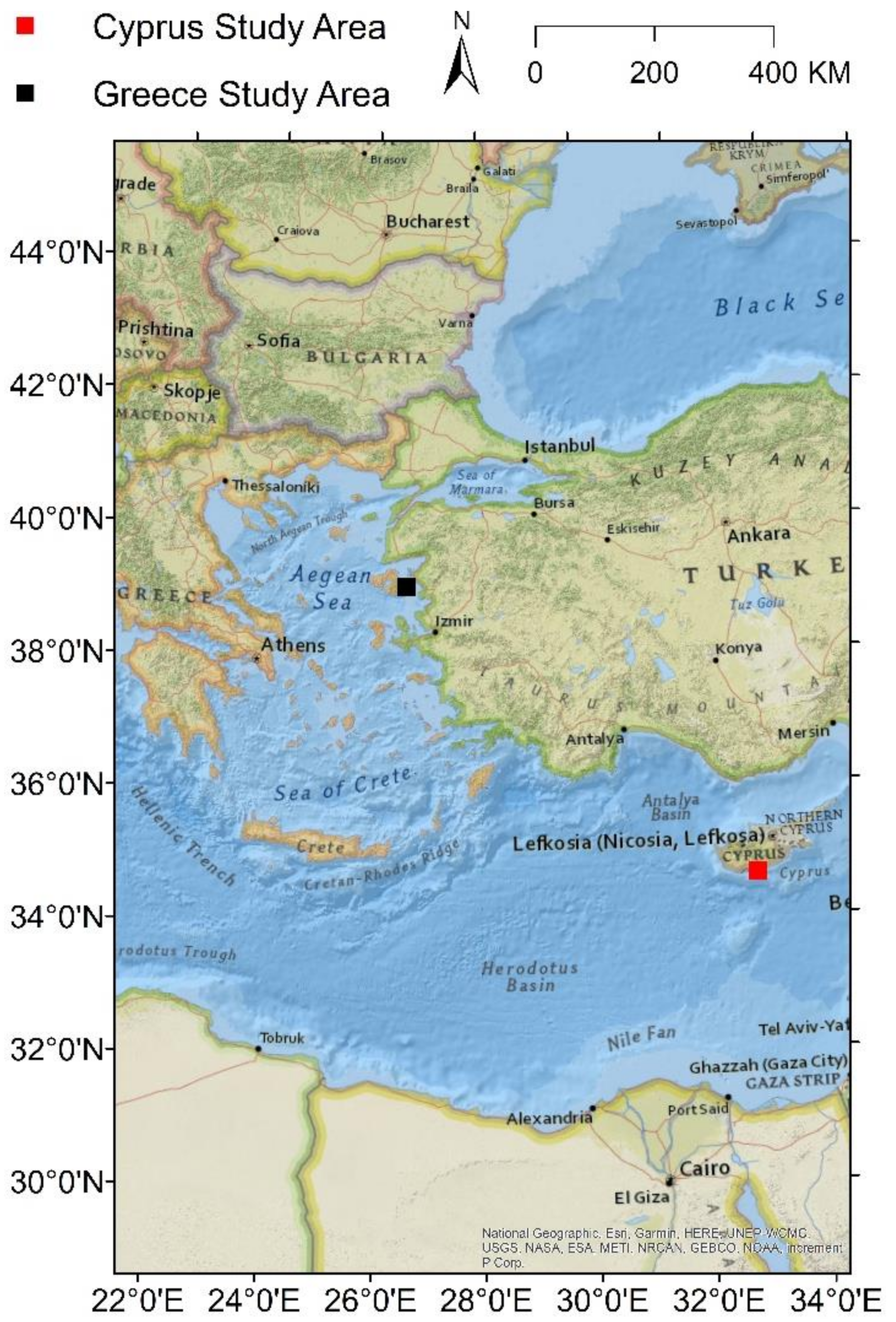
The objective of this study is to detect floating plastics based on freely available, optical remote sensing satellite data. Detection of floating plastics in coastal waters can be performed using a variety of classification algorithms. However, it is not known a priori which of those algorithms are better suited for the analysis. This study considers four classification algorithms to detect floating plastics using Sentinel-2 remote sensing and in situ data and compares the performance of each of these algorithms. Furthermore, the classification algorithms can be developed based on all or a subset of the multi-spectral band data obtained from the optical satellite sensors as well as a set of indices that can be derived from the satellite data. Since the best combination of the bands and indices were not known a priori, this study considered several combinations of multi-spectral bands and indices to identify the optimal combinations to detect floating plastics in coastal waterbodies. To compare the results obtained by using different classification algorithms and bands and indices combinations, real-world, in situ data that was not considered in the development of the classification algorithm needed to be used for the performance evaluation of each developed model. For this purpose, two locations (Limassol, Cyprus and Mytilene, Greece) were identified where in situ experimental data on floating plastics in the coastal water were available. Details on the Sentinel-2 data and in situ data on the chosen two locations are described in Section 2. Section 3 provides details on the four classification algorithms used in the study and the performance evaluation. Results and the discussion are provided in Section 4 and Section 5, respectively, while conclusions are drawn in Section 6.

2. Data Description

The Sentinel-2 remote sensing data were obtained from the Copernicus database at two locations (Limassol, Cyprus and Mytilene, Greece) where in situ data on plastic pollution were available. The remote sensing used for the analysis needed to be processed to perform atmospheric corrections before developing classification models. Details on the data, atmospheric correction, and in situ data description are provided below.

2.1. Sentinel-2 Data Details

Sentinel-2A and -2B 12-band Level 1C multispectral imagery (MSI) data was obtained from the Copernicus Open Access Hub (https://scihub.copernicus.eu/, (accessed on 3 March 2021)) covering the coastline of Limassol, Cyprus and Mytilene, Greece. Details on the Sentinel band information and spatial resolution are provided in

Table 1. Central wavelength value for Sentinel-2A and Sentinel-2B satellite multispectral instrument (MSI) bands.

MSI Bands	Description	Sentinel-2A Central Wavelength (nm)	Sentinel-2B Central Wavelength (nm)	Spatial Resolution (m)
Band 1	Coastal Aerosol	442.7	442.3	60
Band 2	Blue	492.4	492.1	10
Band 3	Green	559.8	559	10
Band 4	Red	664.6	665	10
Band 5	Red Edge 1	704.1	703.8	20
Band 6	Red Edge 2	740.5	739.1	20
Band 7	Red Edge 3	782.8	779.7	20
Band 8	Near Infrared (NIR)	832.8	833	10
Band 8A	Narrow NIR	864.7	864	20
Band 9	Water Vapour	945.1	943.2	60
Band 10	Short Wave Infrared (SWIR) Cirrus	1373.5	1376.9	60
Band 11	SWIR 1	1613.7	1610.4	20
Band 12	SWIR 2	2202.4	2185.7	20

. Instead of Level 2A, Level 1C data was used in this study for the following reasons: (i) Level 2A data provides the system-generated bottom of atmosphere (BOA) reflectance after processing the Level 1C top of atmosphere (TOA) reflectance using the European Space Agency (ESA) default Sen2Cor atmospheric correction processor. The ESA’s Sen2Cor processor has been found ineffective and performed poorly over the open ocean and coastal waters, while the same has performed well over land areas [36,37,38,39,40]. Since the Sen2cor atmospheric correction processor has been developed based on land-based parameters, it has been recommended not to use it for sea and open ocean areas [40]. (ii) The atmospheric correction and other pre-processing (masking, subset, etc.) of Sentinel Level 1C data were performed using the ACOLITE atmospheric correction processor [38]. Since Level 1C TOA is the default input requirement for the ACOLITE processor, the present study uses only the Level 1C product to cluster and classify floating objects.

A total of 5 Sentinel images (1 for Limassol and 4 for Mytilene) were obtained for analysis in the present study. The Sentinel-2 images were obtained on the same date on which the in situ, real-world plastic pollution data were collected through experiments at the two study area locations. Details on the 5 Sentinel-2 images are provided in

Table 2. Description of the Sentinel-2 images used in the study at two locations along with date of acquisition (dd/mm/yyyy) and product type.

Location	Image Description	Date of Acquisition	Product Type
Limassol, Cyprus	S2A_MSIL1C_20181215T083341_N0207_R021_T36SWD_20181215T085809	15/12/2018	L1C
Mytilene, Greece	S2A_MSIL1C_20180607T085601_N0206_R007_T35SMD_20180607T110513	07/06/2018	L1C
	S2B_MSIL1C_20190418T085559_N0207_R007_T35SMD_20190418T110441	18/04/2019	L1C
	S2A_MSIL1C_20190503T085601_N0207_R007_T35SMD_20190503T103221	03/05/2019	L1C
	S2B_MSIL1C_20190607T085609_N0207_R007_T35SMD_20190607T110335	07/06/2019	L1C

.

Out of the 12 bands of data, only 6 of them were used for analysis in detecting floating plastics in the waterbodies. The selected bands were blue (Band 2), green (Band 3), red (Band 4), red edge 2 (RE2) (Band 6), near infrared (NIR) (Band 8), and short wave infrared 1 (SWIR1) (Band 11). It can be noted from Table 1 that out of those selected 6 bands, 4 of them (blue, green, red, and NIR) have a spatial resolution of 10 m, while the other 2 (RE2 and SWIR1) have a spatial resolution of 20 m. The coarser resolution band images were resampled to 10 m resolution by using bi-linear interpolation before performing classification analysis.

2.2. Performing Atmospheric Correction

The present study utilizes the ACOLITE [37,38] atmospheric correction processor developed by the Royal Belgian Institute of Natural Sciences (RBNS) for the aquatic application of Landsat and Sentinel data. ACOLITE performs atmospheric correction and produces remote sensing surface reflectance (Rrs) using water-based parameters. Exponential extrapolation function (EXP) and dark spectrum fitting (DSF) algorithms are the two main approaches of the ACOLITE processor. Between the two methods, the DSF is preferred and utilized in this study, as it is developed based on the following assumptions: (1) homogenous atmosphere covering a certain aerial extent and (2) the zero reflectance values of specific pixels in at least one sensor band [37,38]. The ACOLITE processor is available in two formats, a graphical user interface (GUI) and a command line interface (CLI) for performing atmospheric correction on the remote sensing images. The GUI has limited functionality and configuration wherein it allows users only to modify the input/output path setting, region of interest, and a number of parameters to be processed. On the other hand, the CLI offers full functionality, processes the uncorrected Landsat/Sentinel images using the metadata file available from the satellite database, and has been used in this study. All of the Sentinel-2 data (provided in Table 2) were processed in ACOLITE to obtain the atmospheric-corrected surface reflectance product for the selected 6 bands.

2.3. Design and Configuration of Plastic Targets in Limassol (Cyprus) and Mytilene (Greece)

In situ data from Limassol, Cyprus and Mytilene, Greece (Figure 1) were considered to verify the accuracy and performance of both unsupervised and supervised plastic detection models developed in this study. The site at Limassol, Cyprus was selected based on reported evidence of accumulation of a large amount of plastic debris from the ships in this region [41,42,43]. Themistocleous et al. [41] conducted an experimental study on plastic detection in Limassol, Cyprus, in which they deployed targets made of plastic near the Old Port of Limassol on 15 December 2018 to examine if the plastic litter could be detected through Sentinel-2 satellite images. For this purpose, a 3 m × 10 m plastic litter target was created using 0.5 litre and 1.5 litre-sized water bottles and was floated in the coastal water in Limassol. In total, the target covered 4 Sentinel-2 grids as shown in Figure 2a. To be the best of our knowledge, this type of experiment was first conducted by Topouzelis et al. [35] on 7th June 2018 at the Tsamakia Beach, Mytilene, Greece, where they deployed a 10 m × 10 m plastic target. The target was created using 3600 polyethylene terephthalate bottles, each having a size of 1.5 litres, as well as plastic bags and fishnets. In total, the target covered 12 Sentinel-2 grids (Figure 2b). A similar experiment was conducted by Topouzelis et al. [44] at the same location between April and June 2019 multiple times. On 18th April 2019, they deployed 4 5 m × 5 m plastic targets in which the targets were created by using plastic bottles (50% volume) and plastic bags (50% volume). Overall, the plastic targets covered 6 Sentinel-2 grids (Figure 2c). On 3 May 2019, the University of Aegean team placed 4 5 m × 5 m plastic targets at far distances from one another. Additionally, 2 1 m × 10 m targets were also deployed along with the 4 main targets on that day. One of the additional targets was made of plastic bottles, and the other one was prepared by using a combination of plastic bags and plastic mesh. A total of 25 Sentinel-2 (Figure 2d) grids were identified for this date covering plastic objects. The team conducted another experiment on 7th June 2019 using 4 5 m × 5 m plastic targets that covered 12 Sentinel-2 grids (Figure 2e). Data used for Limassol, Cyprus were available from Themistocleous et al. [41], while the data used for Mytilene, Greece were available at the link https://zenodo.org/record/3752719#.YEE8oGj7RPZ, (accessed on 3 March 2021). Further details on the database creation can be found in Themistocleous et al. [41].

It needs to be noted that the days on which the experiments at Limassol, Cyprus and Mytilene, Greece were conducted were selected by keeping in mind that either Sentinel-2A or Sentinel-2B would fly by the study area on the same day.

3. Methodology

The goal of this study was to identify the presence of floating plastics in a sea/ocean waterbody using Sentinel-2 remote sensing imagery. This study considered the use of two unsupervised classification/clustering algorithms and two supervised classification algorithm to detect floating plastics in coastal waters by using the Sentinel-2 remote sensing data. The supervised classification algorithms required a predefined training dataset wherein information on the presence/absence of floating plastics in a set of grids in the waterbody was available based on in situ data. The training dataset was used to calibrate the model parameters of the supervised classification. Once the model was calibrated and validated, it could be used to detect the presence of floating plastics in other grids in the study area that did not belong to the training dataset. On the other hand, the development of an unsupervised classification algorithm (also termed as unsupervised clustering) used only the remote sensing data and did not require any in situ prior information to develop the model. In situations where limited/no training data are available, unsupervised clustering is the only option to develop a model to detect floating plastics in a waterbody. Since real-world information is being used to develop the supervised classification algorithm, it is expected that the performance would be better for detecting floating plastics when compared to unsupervised classification models.

The two clustering algorithms used for unsupervised classification were K-means hard clustering and fuzzy c-means (FCM) clustering. In the literature, these two approaches are found to be robust in forming clusters [45,46]. The supervised classifications considered in this study were the support vector regression (SVR)-based algorithm and the semi-supervised fuzzy c-means (SFCM) algorithm. The major advantage of the SVR model is that it can quantify nonlinear relationships between the set of predictors and predictand using a kernel function [47]. The SFCM is a modification of the unsupervised FCM in which information on the classification is used to form clusters [48,49]. In the case of supervised classification, the predictors in the modelling were the Sentinel-2 data obtained at different bands/wavelengths, while the predictand was the presence/absence of floating plastic in a chosen grid/location in the waterbody. Since the optimal combination of Sentinel-2 bands data to produce the highest efficiency in detecting floating plastics in a waterbody was not known a priori, different combinations of available remote sensing band data and a set of indices that were found to be useful in detecting floating plastics were considered in this study. Subsequently, the best-suited algorithm and best combinations of bands and indices were identified to detect floating plastics at an arbitrary location using the Sentinel-2 dataset.

The literature revealed [50] that a newly proposed index called the Floating Debris Index (FDI) was useful in the identification of floating plastics in waterbodies using remote sensing imagery. The FDI can be estimated as:

$$\mathrm{FDI}=R_{\mathrm{NIR}}-R^{\prime }{}_{\mathrm{NIR}}$$

(1)

$$R^{\prime }{}_{\mathrm{NIR}}=R_{\mathrm{RE}2}+\left(R_{\mathrm{SWIR}1}-R_{\mathrm{RE}2}\right)\times \frac{{\lambda }_{\mathrm{NIR}}-{\lambda }_{\mathrm{RED}}}{{\lambda }_{\mathrm{SWIR}1}-{\lambda }_{\mathrm{RED}}}\times 10$$

(2)

where $R_{\mathrm{NIR}}$, $R_{\mathrm{RE}2},$ and $R_{\mathrm{SWIR}1}$ denote the reflectance values measured using the satellite per grid corresponding to near infrared (NIR), red edge 2 (RE2,) and short wave infrared 1 (SWIR1) bands, respectively. ${\lambda }_{\mathrm{NIR}}$, ${\lambda }_{\mathrm{RED},}$ and ${\lambda }_{\mathrm{SWIR}1}$ are, respectively, the central wavelengths (in nanometres) corresponding to the NIR, red and SWIR1 bands measured by the satellite. The central wavelengths corresponding to different bands for the Sentinel-2 satellite are provided in Table 1.

Another index that was found to be useful in detecting plastics was the Normalized Difference Vegetation Index (NDVI), given as:

$$\mathrm{NDVI}=\frac{R_{\mathrm{NIR}}-R_{\mathrm{RED}}}{R_{\mathrm{NIR}}-R_{\mathrm{RED}}}$$

(3)

Biermann et al. [50] considered the two indices FDI and NDVI along with the reflectance values obtained for the bands red, red edge 2, NIR, and SWIR1 and developed a naïve Bayesian model to predict the presence of floating plastics in waterbodies using Sentinel-2 data. Since the algorithm was a supervised classification algorithm, it required a set of training databases wherein the presence/absence of plastics in a set of grids needed to be used to estimate the model parameters.

The development of the classification model to predict the presence/absence of floating plastics required a set of attributes that were useful in detecting floating plastics. From a literature review [50], it has been found that the FDI takes a high value and the NDVI takes a low value in grids with the presence of floating plastics. Furthermore, reflectance values corresponding to bands red, NIR, RE2 and SWIR1 have also been used, as they have been found to be useful for detecting floating plastics. However, the optimal band combinations to produce the highest efficiency in detecting floating plastics in waterbodies were not known a priori. This study considers three combinations of bands/indices to develop the attribute sets and perform supervised and unsupervised classification. The three attribute sets considered in this study are shown in

Table 3. Details of attribute sets used for classification.

Attribute Set	Bands/Indices Used
A	(i) Blue, (ii) Green, (iii) Red, (iv) RE2, (v) NIR, and (vi) SWIR1, and two indices (vii) FDI, and (viii) NDVI
B	(i) Red, (ii) RE2, (iii) NIR, and (iv) SWIR1, and two indices (v) FDI, and (vi) NDVI
C	(i) FDI and (ii) NDVI

.

Details of the four classification algorithms and their performance evaluations are provided in the following subsections.

3.1. K-means Clustering Algorithm

This section presents a K-means clustering method [51] that yield hard clusters through a deterministic search procedure. The method assumes that points in the attribute space can be segregated by using straight lines or linear planes and that the points can be segregated into clusters such that points in a cluster fully resemble each other and those in different clusters do not have any resemblance.

Let $x_s=\left[x_{s,1},\cdots ,x_{s,m}\right]\in {\mathcal{\Re }}^m$ denote a vector containing $m$ attributes for a grid $s \left(1,\cdots ,N\right)$, with $x_{s,j}$ representing the value of the $j$th attribute for the grid. The attribute can be the reflectance value corresponding to a given remote sensing band (e.g., blue, green, red, NIR, SWIR1, etc.) or value of an index (e.g., FDI, NDVI) at the grid $s$. Once the attribute values for each site are obtained, a feature matrix $X={\left[x_1,\cdots ,x_N\right]}^T$ containing vectors from all the sites can be prepared.

The K-means algorithm partitions the feature matrix $X$ into $K_{opt}$ number of clusters by minimizing the following objective function:

$$\mathrm{Minimize}F\left(X,V:K\right)={\displaystyle \sum }_{s=1}^N{\displaystyle \sum }_{i=1}^{K}I\left(x_s\in C_i\right)\times d^2\left(x_s,v_i\right)$$

(4)

where $C_i$ denote the i-th hard cluster, $I\left(·\right)$ is an indicator function where $I=1$ if $\left(x_s\in C_i\right)$ is true and $I=0$ otherwise; $V={\left[v_1,\cdots ,v_K\right]}^T$ is a matrix containing centroids of K clusters such that $v_i=\left[v_{i,1},\cdots ,v_{i,m}\right]\in {\mathcal{\Re }}^m$ and $d^2\left(·,·\right)$ is the square of the Euclidean distance between two vectors.

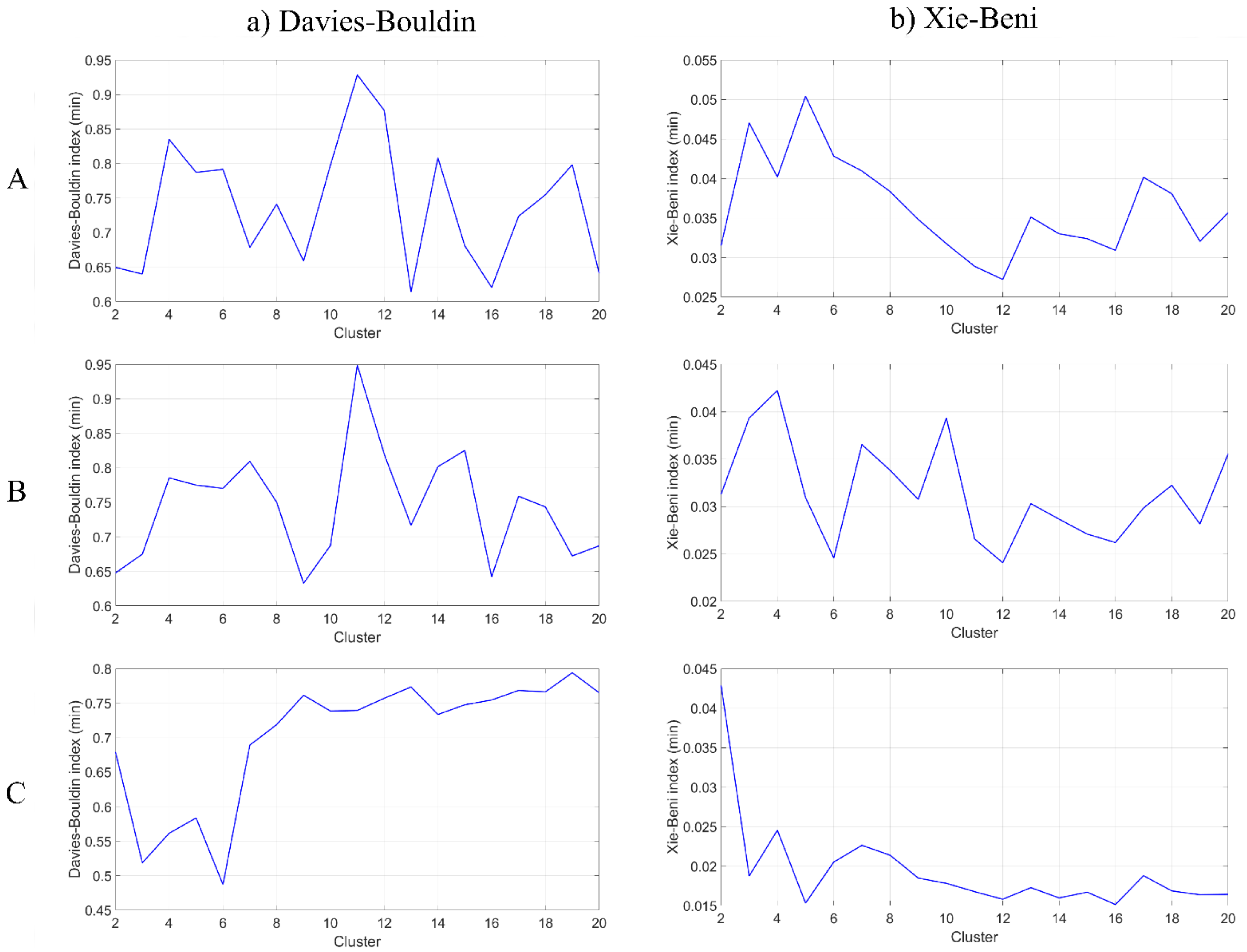
The optimal number of clusters $K_{opt}$ can be identified using the Davies–Bouldin ($DBI$) cluster validity index [52]. The index is a function of the ratio of the sum of within-cluster scatter to between-cluster separation and is computed as:

$$DBI\left(K\right)=\frac{1}{K}{\displaystyle \sum }_{i=1}^K\underset{i,i\ne l}{\max }\left\{\frac{Scatte{r}_i+Scatte{r}_l}{d_{i,l}}\right\}$$

(5)

where $Scatte{r}_i$ and $Scatte{r}_l$ are within cluster scatter for the i-th and l-th clusters, respectively. In general, $Scatte{r}_i$ is computed as $Scatte{r}_i=\sqrt{{\displaystyle \sum }_{x_s\in C_i}{x}_s-v_i{}^2/N_i}$; $N_i$ is the number of points in cluster i and $d_{i,l}$ is the Euclidean distance between the centroids of the i-th and l-th clusters. A feature vector can be assigned to the cluster whose centroid is closest to the vector. Optimal clusters should have the lowest $DBI$ value.

3.2. Fuzzy c-means Clustering Algorithm

This section presents a fuzzy c-means (FCM) clustering method [53] that is designed to be useful in real world scenarios where a chosen grid may be partially filled with floating plastics. Let N denote the number of feature vectors prepared as described in Section 3.1. To form clusters, the FCM method involves partitioning of the feature matrix $X={\left[x_1,\cdots ,x_N\right]}^T$ into c clusters by executing the following steps. The method attempts to minimize the following objective function:

$$\mathrm{Minimize}J\left(U,V:X\right)={\displaystyle \sum }_{i=1}^c{\displaystyle \sum }_{s=1}^N{\left(u_{s,i}\right)}^{\mu }\times d^2\left(x_s,v_i\right)$$

(6)

subject to the following constraints,

$${{\displaystyle \sum }}_{i=1}^c{u}_{s,i}=1 \forall s\in \left\{1,\cdots ,N\right\}\mathrm{and}0<{{\displaystyle \sum }}_{s=1}^N{u}_{s,i}<N \forall i\in \left\{1,\cdots ,c\right\}$$

(7)

where $U=\left\{u_{s,i},i=1,\cdots ,c;s=1,\cdots ,N\right\}$ is the fuzzy partition matrix in which $u_{s,i}\in \left[0,1\right]$ denotes the membership of $x_s$ in the i-th fuzzy cluster, $V={\left[v_1,\cdots ,v_c\right]}^T$ is a matrix containing centroids of c clusters in the m-dimensional feature space such that $v_i=\left[v_{i,1},\cdots ,v_{i,m}\right]\in {\mathcal{\Re }}^m$, $\mu \in \left(1,\infty \right)$ refers to the fuzzifier that depicts fuzziness of the clusters, and $d\left(·,·\right)$ is the Euclidean distance between two vectors. The memberships tend to either 1 or 0 as the value of $\mu$ tends to 1.

The optimal number of clusters and optimal fuzzifier value can be identified for situations where the value of Xie-Beni cluster validity index $V_{XB}$ [54] is minimal.

$$V_{XB}\left(U,V:X\right)={\displaystyle \sum }_{i=1}^c{\displaystyle \sum }_{s=1}^N{\left(u_{s,i}\right)}^{\mu }||x_s-{v_i\left|\right|}^2/N\underset{l,l\ne i}{\min }||v_l-{v_i\left|\right|}^2$$

(8)

3.3. Support Vector Regression (SVR) Algorithm

The support vector regression (SVR) develops a nonlinear relationship [55] between an input vector $x_s=\left[x_{s,1},\cdots ,x_{s,m}\right]\in {\mathcal{\Re }}^m$ and output $y_s\in \mathcal{\Re }$.

The relationship can be expressed as:

$$y_s=f\left(x_s\right)+e\left(t\right)$$

(9)

where $\left\{f\left(\cdot \right);{\mathcal{\Re }}^m\to \mathcal{\Re }\right\}$ is a nonlinear transformation function [55] and $e\left(t\right)$ is white noise whose expected value $E\left[e\left(t\right)\right]$ is 0. The relationship is developed based on n number of training data where the presence of floating plastic for grid s is known. In this study,

$$y_s=\left\{\begin{array}{c}0,\mathrm{when}\mathrm{the}\mathrm{grid}\mathrm{has}\mathrm{no}\mathrm{plastic}\\ 1,\mathrm{when}\mathrm{the}\mathrm{grid}\mathrm{has}\mathrm{plastic}\end{array}\right., \forall s=\left\{1,\cdots ,n\right\}$$

(10)

Details of the SVR algorithm can be found in Vapnik [55].

3.4. Semi-Supervised Fuzzy c-means (SFCM) Algorithm

The semi-supervised fuzzy c-means (SFCM) algorithm is an extension of the FCM clustering wherein a portion of the data, termed as a training set that is used for clustering, are known to belong to a given cluster a priori [48]. The SFCM algorithm is a hybrid clustering algorithm which can extract the hidden pattern present in the data by using FCM clustering on the non-trained data and use the training data to improve the cluster formation. The SFCM algorithm minimizes the following objective function:

$$J\left(U,V:X\right)={\displaystyle \sum }_{i=1}^c{\displaystyle \sum }_{s=1}^N{\left(u_{s,i}\right)}^{\mu }\times d^2\left(x_s,v_i\right)+\alpha {\displaystyle \sum }_{i=1}^c{\displaystyle \sum }_{s=1}^N{\left(u_{s,i}-f_{s,i}{b}_s\right)}^{\mu }\times d^2\left(x_s,v_i\right)$$

(11)

where $\alpha$ is a scaling factor that maintains balance between the training and non-training data, $f_{s,i}$ are the membership values of the training dataset, and $b_s$ is a Boolean indicator that takes a value equal to 1 if the data belongs to a training set and zero if the data is non-trained.

3.5. Performance Evaluation

In order to evaluate the performance of a chosen algorithm for detecting the floating plastics in coastal waterbodies, the total available training data needed to be subdivided into two sets. The first set, termed the calibration set, was used to develop the model using a chosen algorithm (either supervised or unsupervised) and estimate the model parameters. Subsequently, the developed model was implemented for the remotely sensed bands and indices to predict presence/absence of floating plastics in grids belonging to the second set, called the validation set. Subdividing the total training data into the calibration and validation sets was necessary to ensure that the validation set data that were used for performance evaluation of the model had not been used to develop the model.

The effectiveness of the classification approach in detecting presence/absence of floating plastics was evaluated in terms of the error/confusion matrix, overall accuracy, and F-score statistic based on the validation set data. The error matrix consisted of 2 rows and 2 columns (

Table 4. Structure of an Error/Confusion Matrix.

Error Matrix	Observed
Model predicted	Plastic	No Plastic
Plastic	True positive (TP)	False positive (FP)
No Plastic	False negative (FN)	True negative (TN)

). Along the row-wise direction, the observed/in situ information on the presence/absence of floating plastics was indicated, while in the column-wise direction, the model predicted values were noted. In situations where the model predicted the presence/absence of floating plastic at the grid where in situ observations agreed with the predictions, the algorithm could be considered to be efficient. In the error matrix, true positive (TP) indicates that the model correctly predicts the presence of floating plastics, while true negative (TN) means the model correctly predicts the absence of floating plastic in a grid. On the other hand, false positive (FP) means the model wrongly predicts the presence of floating plastic in a grid where plastic is absent based on the in situ ground truth data, whereas false negative (FN) indicates the algorithm fails to detect floating plastic in a grid.

The overall accuracy could be estimated by summing the number of grids where the model predicted correctly and dividing that value by the total number of grids. Based on the table, the overall accuracy = 100 × (TP + TN)/(TP + TN + FP + FN). The overall accuracy ranges from 0 to 100%.

Subsequently, the F-score can be estimated based on the results as:

$$\mathrm{F}-\mathrm{score}=\frac{\mathrm{TP}}{\mathrm{TP}+\frac{1}{2}\left(\mathrm{FP}+\mathrm{FN}\right)}$$

(12)

The F-score value ranges from 0 to 1. In situations where the model performance was better, the overall accuracy tended toward 100% while the F-score approached unity.

4. Results

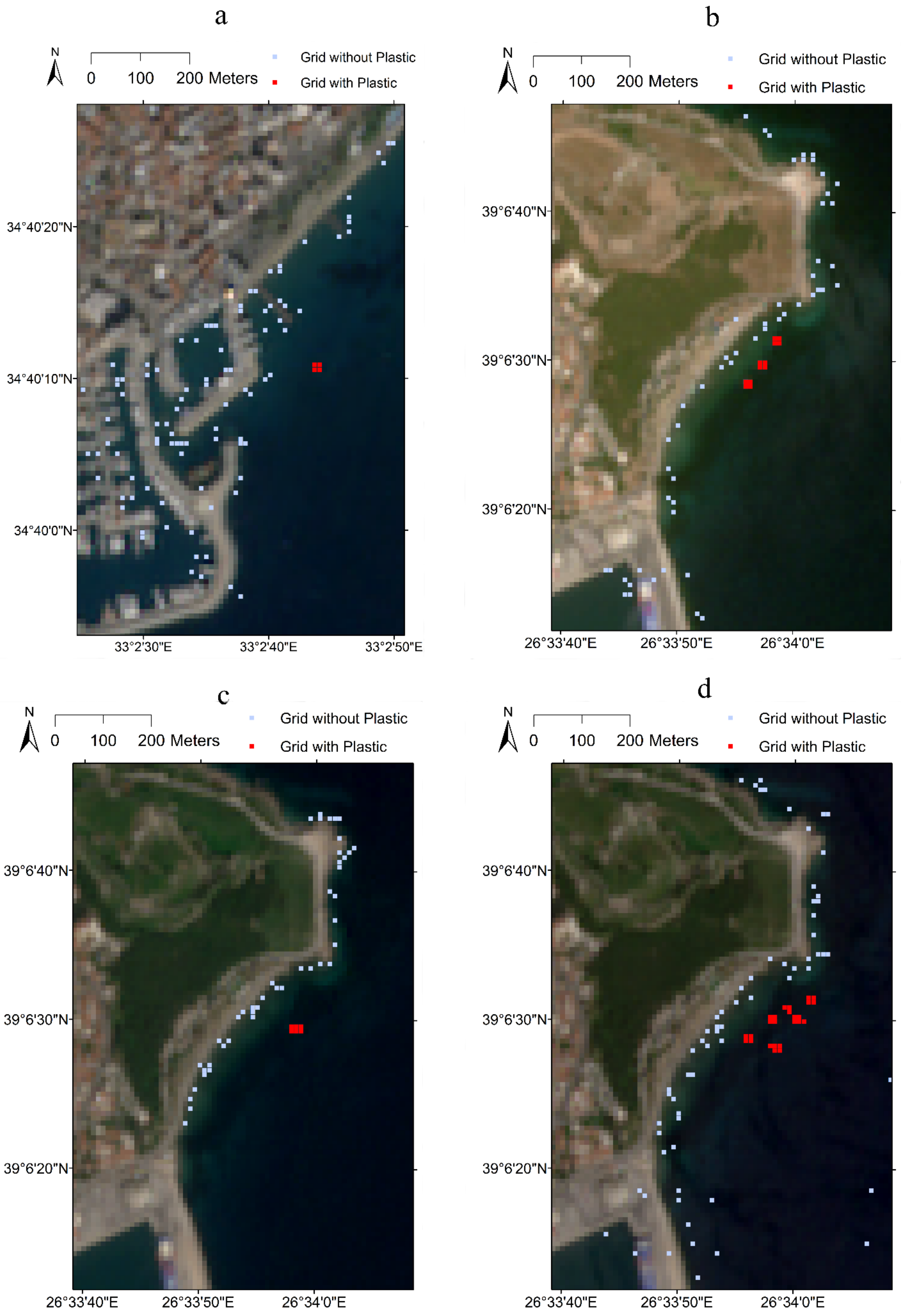
This study considered data from two locations, Limassol, Cyprus and Mytilene, Greece, to investigate the effectiveness of the four classification algorithms. The reason for selecting those two locations was that a real-world experiment was performed in the coastal waters of those two locations and the presence of floating plastics was verified by using in situ observations. 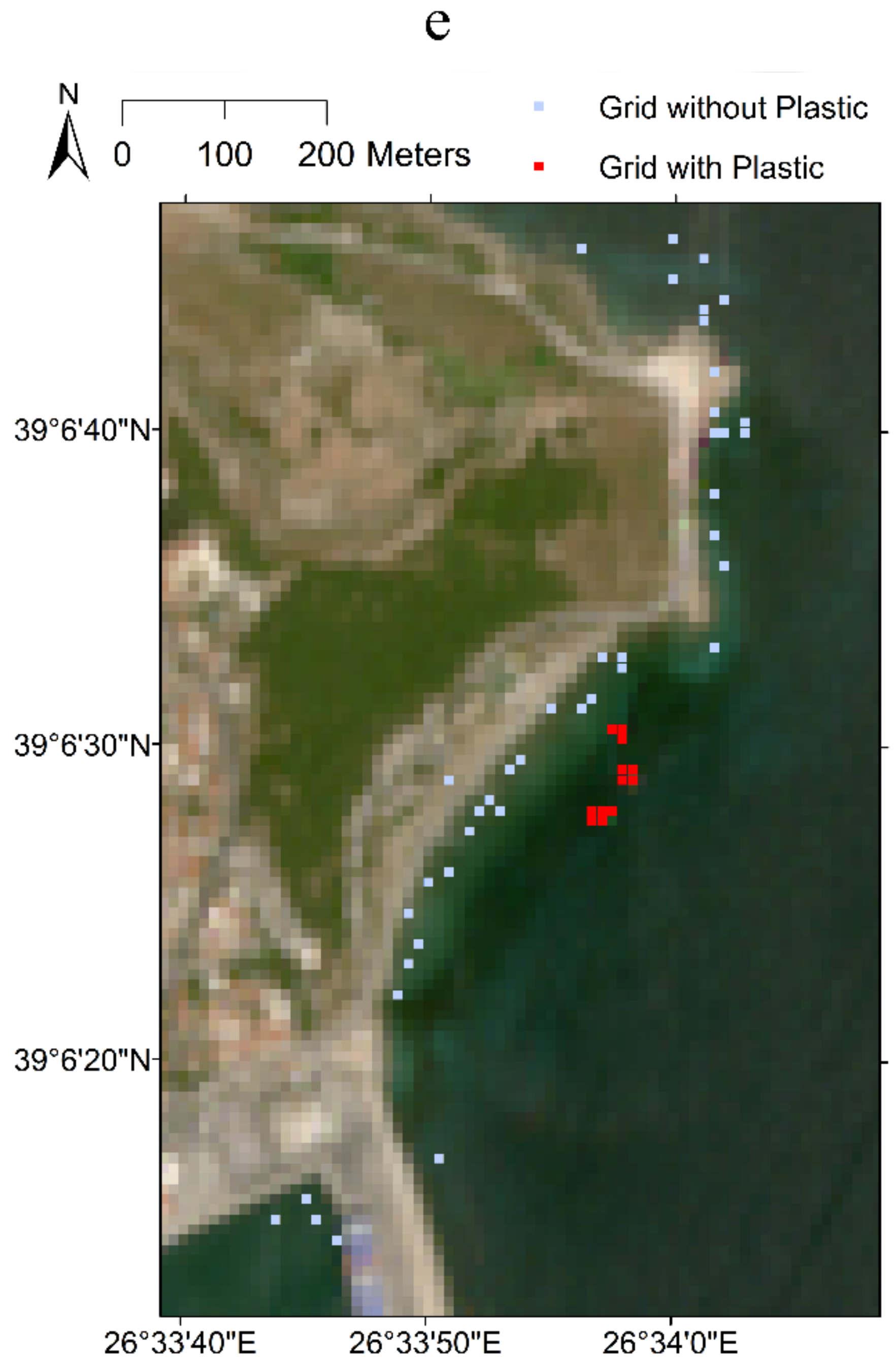In Limassol, plastics were detected in 4 grids on 15 December 2018 based on in situ observations, while clear water was detected in 95 grids based on aerial and Sentinel images (Figure 2a). Similarly, in Mytilene, in situ floating plastic was detected in 12, 6, 25, and 12 grids respectively on 7 June 2018, 18 April 2019, 3 May 2019, and 7 June 2019, respectively (Figure 2b–e). The number of grids with clean water at Mytilene on the aforementioned four dates were 92, 86, 94, and 91 respectively. Based on the in situ database, 59 grids were identified to have floating plastics, while based on aerial and Sentinel images, 458 grids were found to have clean water without the presence of floating plastics. In total, the training dataset consisted of 517 grids. In this study, 75% of the entire training data were considered as the calibration set, and the remaining 25% data was selected as the validation set. The calibration set consisted of 388 grid data points, and the validation set had 129 grids. Based on in situ information, it was noted that out of 388 grids, 44 grids had floating plastics, whereas the remaining 344 grids did not contain any plastic. It can be noted that the supervised SVR algorithm has been developed based on the 388-grid calibration set data, whereas the remaining 129-grid data, in which 15 grids had floating plastics and the remaining 114 grids did not have plastics, were solely used for performance evaluation.

The total number of 28,797 unsupervised/untrained grids have been considered in the study along with the 517 trained grids. The untrained grids were located within a distance of 500 m from the grids where floating plastic was detected. Those grids were considered to be untrained, as in situ information on floating plastic at those grids was unknown; however, the reflectance values and the FDI and NVDI values at each of the grids were available from the Sentinel-2 remote sensing data. This untrained database of 28,797 grids was combined with the 388 grid data from the calibration set to perform the two unsupervised classifications and the semi-supervised fuzzy c-means classification. The reason for using the untrained data was that both K-means and FCM algorithms, as well as the SFCM algorithm, require a considerable number of datasets to form clusters. Since the SVR-based supervised classification algorithm cannot use an untrained database for parameter estimation, the SVR model was developed by using data from the calibration set only.

A comparison of the performance of each of the four classification algorithms with the three different attribute sets A, B, and C was investigated using the 129-grid validation set data. The classification algorithm could be considered to perform correctly when it predicted the presence of floating plastics in grids where plastic was found to be present by using in situ data. In addition, the algorithm worked properly when it did not detect floating plastics in clean water. Error occurred when the algorithm failed to detect floating plastics in grids where they were present or predicted the presence of floating plastics in clean water.

Based on the untrained dataset and the calibrating data, the K-means clustering algorithm was developed by separately using the three attribute sets A, B, and C. Since the optimal number of clusters were not known a priori, the cluster values K ranging from 2 to 20 were considered, and the clusters were formed. The optimal cluster numbers K_opt were identified based on the Davies–Bouldin cluster validity index (Figure 3a). The optimal K-means cluster numbers were found to be 13, 9, and 6 for attribute sets A, B, and C, respectively. Based on the analysis, the clusters that represented the floating plastics were identified, and the cluster centroids were noted. Based on the cluster centroids, the data from the validation set were reclassified to predict the presence/absence of floating plastics. A performance matrix (error/confusion matrix) was developed to estimate the performance of the algorithm in predicting the presence/absence of floating plastics. The performance matrix based on K-means clustering using each of the three attribute sets is shown in

Table 5. Performance/confusion matrix based on the validation set data using (a) K-means, (b) fuzzy c-means (FCM) and (c) support vector regression (SVR)-based algorithms by considering three different attribute sets A, B, and C, where OA denotes overall accuracy. The numbers in the confusion matrix indicate the number of grids in the validation set belonging to each category.

Algorithm	Attribute	A				B				C
	Modelled	Observed		OA (%)	F-Score	Observed		OA (%)	F-Score	Observed		OA (%)	F-Score
		Plastic	No Plastic			Plastic	No Plastic			Plastic	No Plastic
K-means	Plastic	12	21	81.4	0.50	12	25	78.3	0.46	12	36	69.8	0.38
	No Plastic	3	93			3	89			3	78
FCM	Plastic	13	21	82.2	0.53	12	21	81.4	0.50	12	36	69.8	0.38
	No Plastic	2	93			3	93			3	78
SVR	Plastic	13	0	98.4	0.93	12	0	97.7	0.89	11	0	96.9	0.85
	No Plastic	2	114			3	114			4	114
SFCM	Plastic	14	45	64.3	0.38	14	45	64.3	0.38	2	21	35.7	0.05
	No Plastic	1	69			1	69			13	44

. The overall accuracies obtained using K-means clustering were found to be 81.4%, 78.3%, and 69.8%, respectively, while using attribute sets A, B, and C, and for those sets, the algorithm wrongly predicted 21, 25, and 36 times the presence of plastics at locations where plastic was absent in the real-world scenario. The F-scores for the three attribute sets were found to be 0.5, 0.46, and 0.38, respectively.

Similar to the K-means clustering, the fuzzy c-means (FCM) clustering algorithm was applied to each of the three attribute sets to form clusters. Since the optimal number of clusters and the optimal fuzzifier values were not known a priori, the clustering was performed by considering a different combination of those values. In this study, the cluster number varied from 2 to 20. However, since the objective was to identify whether plastic was present/absent in a chosen grid, a fuzzifier value closer to 1 needed to be considered because a higher fuzzifier value tended to assign nearby membership to all clusters. Hence, the fuzzifier value was not varied, and a single value equal to 1.05 was selected for the analysis. The optimal cluster number was identified based on the Xie–Beni cluster validity index (Figure 3b) and was found to be 12, 12, and 5 for attribute sets A, B, and C, respectively. Following this, the performance matrix was estimated using the validation set data (Table 5). While using attribute sets A, B, and C, the overall accuracy was estimated as 82.2%, 81.4% and 69.8%, respectively. It can be noted that the accuracy was slightly better than that obtained from K-means clustering while using attribute sets A and B, whereas both the clustering algorithms produced similar results when only the indices (attribute C) were used for model development. The number of times the FCM predicted the presence of plastics in grids where plastic was not present in reality were 21, 21, and 36 for sets A, B, and C respectively. The F-score for the three cases using FCM was found to be 0.53, 0.5, and 0.38 respectively.

The support vector regression(SVR)-based supervised classification algorithm was developed based on the calibration data only. The SVR model had two parameters, γ and C. Since the optimal values of those parameters were not known a priori, the model was run by selecting different combinations of the two parameter values, and the best-fit model was identified. The values of γ were considered to be 1, 10, 100, and 1000, while the value of C ranged from 0.1 to 10 with an increment of 0.1. The optimal model parameter values were found to be γ_opt = 100, C_opt = 1.1 for attribute set A, γ_opt = 100, C_opt = 1.0 for attribute set B, and γ_opt = 10, C_opt = 1.5 for attribute set C. Once the model was developed, it was used to predict the presence/absence of floating plastic by using the validation set data, and the performance matrix was estimated (Table 5).

Table 5 indicates that out of the 15 grids where floating plastic was found to be present based on in situ observations, the SVR supervised classification algorithm detected the presence of plastics in 13 (86.7% accuracy) grids when reflectance values from 6 bands and the two indices were used. The accuracy in detecting plastics reduced to 80% (12 out of 15 grids) when blue and green band reflectance data was discarded (set B) and to 73.3% (set C) when only the indices were used to develop the SVR model. One point to be noted is that each of the three SVR models that were developed using different attribute sets managed to correctly identify grids where no floating plastic was present. The overall accuracy of the SVR models was 98.4%, 97.7% and 96.9% while using attribute sets A, B and C, respectively. High values of overall accuracy were obtained, as all three models developed based on the SVR algorithm successfully identified all the grids where plastic was absent in real-world scenarios. The F-score values for attribute sets A, B and C using the SVR algorithm were 0.93, 0.89 and 0.95 respectively.

In the case of SFCM classification, only two clusters were formed, as the calibration set training data had only two classes, presence and absence of floating plastics. The error matrix obtained for the validation set data is shown in Table 5. The overall accuracy and the F-score were found to be low for the SFCM classification.

The FCM algorithm also managed to locate 13 grids where plastic was present while using set A data. However, both FCM and K-means algorithms wrongly predicted the presence of floating plastics in several grids where no plastic was present. The performance of both the supervised and unsupervised algorithms was the best when set A was used and the worst when only the indices were considered to develop the algorithm. The performance of K-means and FCM were similar, with FCM being slightly better. In general, the results indicated the use of blue and green band data along with the red, red edge 2, NIR, and SWIR 1 as well as the two indices FDI and NDVI could provide better plastic detection. The supervised classification algorithm was considerably better when compared to unsupervised clustering. However, it needs to be noted that the supervised classification algorithm can only be developed in situations where substantial training data are available.

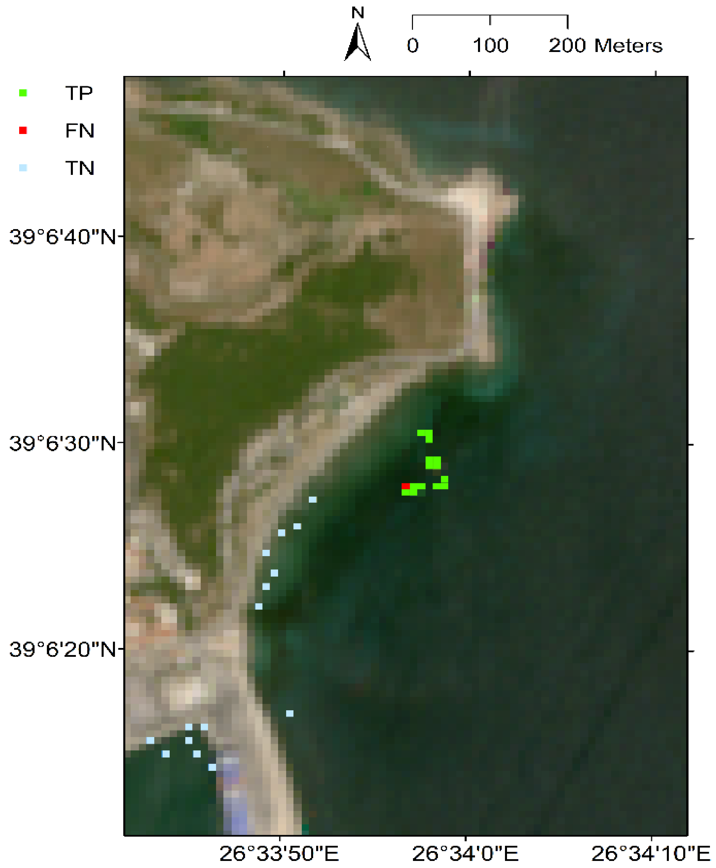
In order to visualize the results, a portion of the validation set data obtained based on in situ observations was plotted in Figure 4. Grids where plastic was found to be present using in situ data are shown in red, while grids with no plastics are shown in blue.

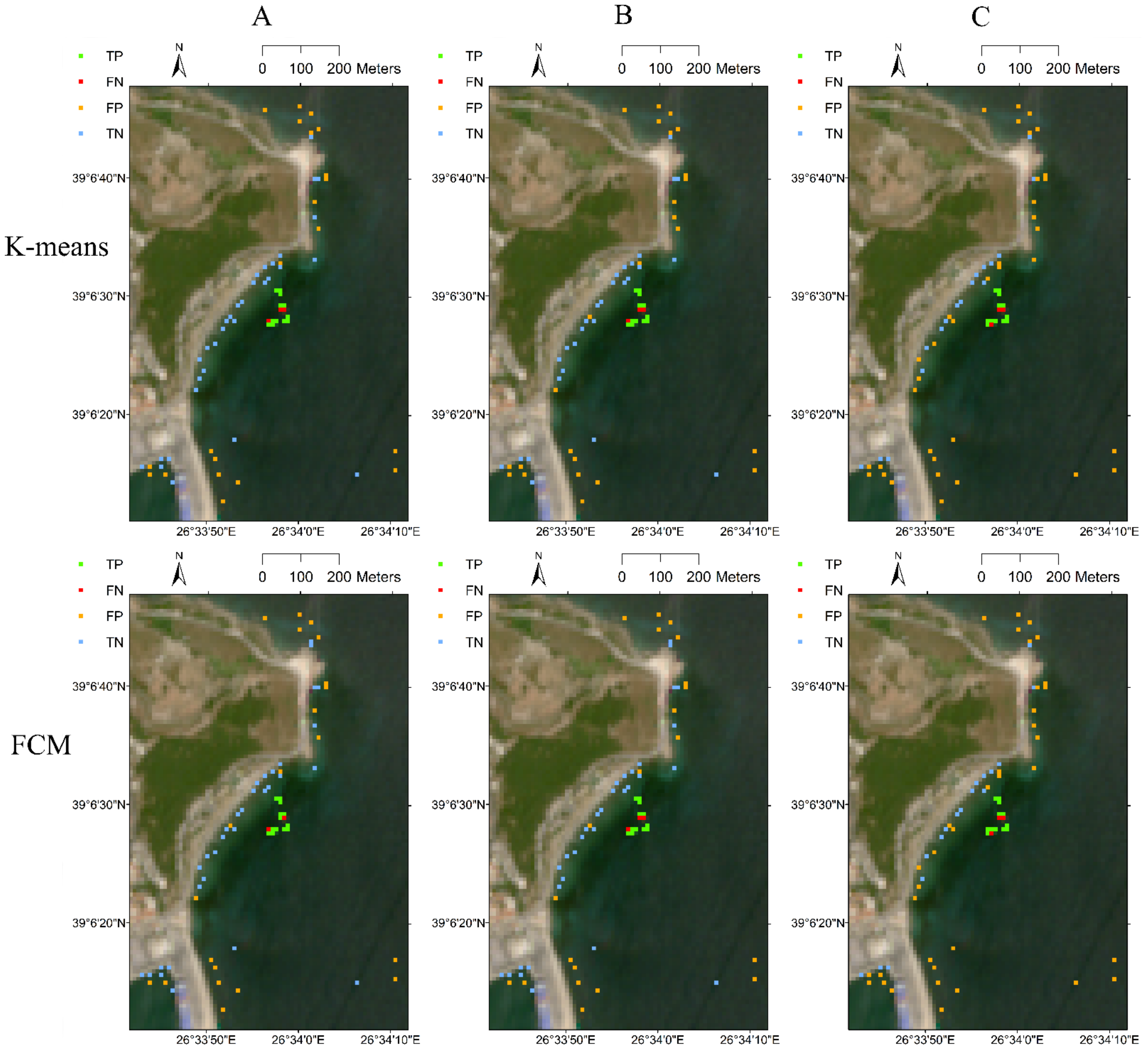
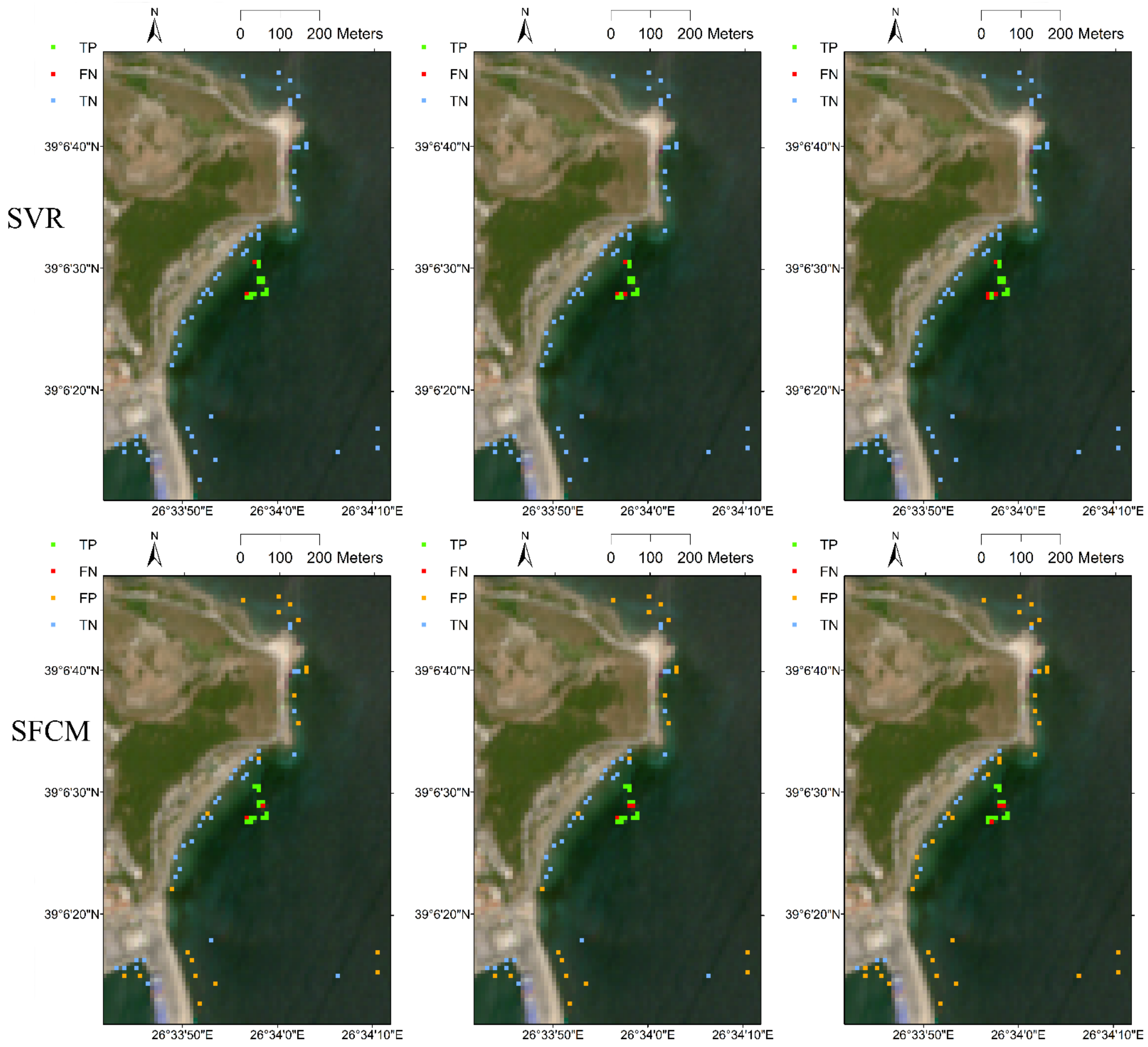
Similar plots were prepared based on classifications obtained using K-means, FCM, SVR and SFCM based classification algorithms and by using each of the three attribute sets A, B, and C (Figure 5). In this figure, grids were plotted as true positive (TP) where the model correctly detected the floating plastics, true negative (TN) where the model correctly predicted the absence of floating plastics, false positive (FP) where the model wrongly predicted the presence of floating plastics, and false negative (FN) where the model failed to detect floating plastics. The figure is useful for locating the correctly classified and misclassified grids from the validation set.

It can be noted from Figure 5 and Table 5 that the supervised SVR algorithm managed to predict the absence of floating plastics in all the grids accurately. One point to be noted here is that in the training dataset that consisted of 517 grids, only 59 of those grids had floating plastics, while the remaining 458 grids had an absence of plastics. The number of grids with floating plastics in the training dataset was considerably low, which may have affected the performance of the developed model. Furthermore, the number of grids without plastic was considerably high (458 grids) when compared to the number of grids with the presence of floating plastics (59 grids). In order to perform a sensitivity analysis, another model was developed wherein an equal number of grids with plastics and without plastics were considered. In the new training data, the existing 59 grids where floating plastics were present were considered, whereas only 59 grids out of the 458 available grids with no plastics were randomly selected to construct the new training set database. Since SVR is the only supervised classification algorithm, it was selected to develop the new mode. Furthermore, as attribute set A was found to provide superior results when compared to attribute sets B and C, only attribute set A was chosen to develop the SVR model. The newly created training set consisting of 118 grid datapoints was subdivided into two sets, the calibration set and the validation set, in a ratio of 3:1. The calibration set consisted of 88 grid points, wherein 44 grids had floating plastics and the remaining 44 grids had no plastics, while the validation set had 30 grid points (15 grids with plastics and 15 without plastics). The performance of the developed model was estimated based on the validation set data and is shown in

Table 6. Error matrix, overall accuracy (OA), and F-score obtained from the SVR model using the validation data consisting of 30 grids.

Algorithm	Modelled	Observed		OA (%)	F-Score
		Plastic	No Plastic
SVR	Plastic	14	0	96.7	0.97
	No Plastic	1	15

and Figure 6.

5. Discussion

Comparative analysis between the two unsupervised clustering algorithms (K-means and fuzzy c-means) and the two supervised classifications (support vector regression and semi-supervised fuzzy c-means) for detecting floating plastics in coastal waterbodies revealed that overall, the supervised classification outperformed the unsupervised clustering algorithm. This can be concluded based on the significant differences in the overall accuracy and the F-score statistic obtained by using the different models. The overall accuracy and the F-score were found to be the highest for the SVR model, followed by FCM, K-means, and the SFCM algorithm. The performance of a chosen classification algorithm for detecting floating plastics by considering the three different attribute sets A, B, and C revealed that all the algorithms performed better when attribute set A was selected to develop the classification model. It can be noted from Table 3 that set A contained reflectance information corresponding to six bands (blue, green, red, NIR, RE2, and SWIR1) as well as two indices (FDI and NDVI). The other two sets, B and C, were subsets of set A and contained less information. The performance of a chosen classification algorithm did not always improve with availability of a higher amount of attribute data. A proper selection of attributes was essential to obtain better performance. A lower number of attributes might not have sufficient information to form effective classifiers, whereas more information might become redundant and mislead the classifiers [56,57]. Superior performance of classification models using set A data indicated that all six bands and the two indices were important and provided independent information to detect the presence/absence of floating plastics in the coastal waterbodies. The reflectance value of waterbodies with and without the presence of floating plastics corresponding to those six bands were different, and they were necessary for the segregation of the grids with plastics from grids without plastics [50].

The validation set consisted of a total of 129 grids, out of which 15 grids had floating plastics, and 114 grids had no plastics present. In situations where attribute set A was considered, the SVR model successfully detected 13 of the 15 grids where plastic was present and failed to detect two grids. However, the algorithm completely detected all the grids with no plastics and did not predict the presence of floating plastics in clear waterbodies. The SFCM algorithm managed to detect 14 grids with plastics; however, it falsely predicted the presence of plastics in clear waterbodies for 45 grids, which led to its poor overall accuracy and F-score. The other two unsupervised algorithms also exhibited several misclassifications wherein the model predicted the presence of plastics in clear waterbodies as well as failed to detect plastics. The SVR model had the advantage of developing nonlinear relationships between the predictor and predictand sets and always reached the global optimal solution while solving the classification algorithm [55], which led to its better performance in detecting floating plastics. The unsupervised classification algorithm was developed solely based on the remote sensing data and did not include information from the training set, which led to its inferior performance. In general, better performance from the SFCM algorithm is expected when compared to that from unsupervised FCM. However, while developing the SFCM clusters, only two clusters were formed in this study, as the calibration set data had only two classes, presence and absence of floating plastics. It can be noted that the SFCM algorithm managed to detect 14 grids with plastics and failed to detect only 1 grid with plastic, while the other algorithms detected 13 or 12 grids and failed to detect 2–3 grids. The error in SFCM arose as it falsely predicted the presence of plastics in clear waterbodies. This is because of the fact that even though those grids did not have plastics present, they may not have been classified as clear water due to the presence of other forms such as seaweed, foam, timber, etc. The performance of SFCM could be considerably improved with better training datasets. Furthermore, it is not definite that the same set of band and index combinations would produce similar accuracy in detecting floating plastics in coastal areas across the world. Detailed research needs to be conducted by performing similar experiments to those conducted in Cyprus and Greece at a global scale to explore the effectiveness of the models used in this study.

Another point to be noted is that the performance of the algorithms was sensitive to the atmospheric corrections applied when processing the Sentinel-2 remote sensing data. In situations where remote sensing images are the solely available data for the identification of floating plastics, the presence of cloud cover and water vapor can be a major issue in obtaining accurate data. The selection of an effective atmospheric correction algorithm for coastal waterbodies is essential to improve the accuracy in detecting floating plastics from remote sensing images.

Another challenge is that most of the open access remote sensing satellite data are available at a spatial resolution of 10 m or coarser range, indicating that one single spectral reflectance value is available over an area of 100 square meters or more. In a real-world scenario, it is extremely likely that floating plastics might be present only in some portion of the area of each remote sensing grid. This makes the detection process extremely challenging. Furthermore, different types of plastics such as bottles, bags, fishnets, etc. would have different reflectance values at multiple wavelengths. Further research needs to be performed to create plastic targets for training datasets wherein a mixture of plastic materials is present and the target covers only a fraction of the remote sensing grids.

6. Conclusions

Based on an advanced machine learning algorithm (support vector regression) and clustering techniques (K-means, fuzzy c-means), the potential application of open source Sentinel data in detecting marine floating plastic at the remote sensing grid scale was thoroughly examined. Despite uncertainties and data limitations, the present research successfully demonstrates the application and functional usability of these machine learning and clustering techniques in detecting floating marine debris. Replicability and easy transferability of the models and approaches have been the key focus of this study. The analysis also demonstrates that the developed models can be used to detect floating plastics across the world as a real-time solution if real-time satellite data can be fed into the algorithms. Additionally, since the algorithms developed in this study are primarily based on remote sensing spectral bands, the same can be applied to any similar remote sensing data (Landsat or other high-resolution satellite data with spectral bands identical to Sentinel-2).

The study investigated the effectiveness of two unsupervised (K-means and FCM) and two supervised classification algorithms (SVR and SFCM) in detecting floating plastics in coastal waterbodies. Based on data from the coastline of Cyprus and Greece, 59 grids were located with the presence of floating plastics. Out of those 59 grids, 44 grids were used to develop the models, while 15 grids were considered as a validation set for performance evaluation of the models. Three different attribute sets were chosen to develop each of the classification models. The biggest attribute set considered 6-band reflectance data from Sentinel-2 images and two indices estimated from the Sentinel-2 data, while the other two attribute sets were subsets of the biggest attribute set. The performance of each of these models was found to be superior when the biggest attribute set was chosen. The model performance was categorized based on its accuracy in identifying grids with plastics and grids without plastics, while the errors in misclassification were also noted. Out of the 15 grids with plastics, SFCM detected 14 grids correctly, SVR and FCM detected 13 grids correctly, and K-means detected 12 grids. The SVR model didn’t predict floating plastic in any grids with clear water; however, the other three algorithms wrongly predicted the presence of plastics in grids where plastic was absent in real world scenarios. It can be noted that some of those grids might exhibit other types of materials such as foam, timber, and seaweed. Further analysis needs to be performed with bigger training samples collected across the world to develop better classification algorithms. Current research is focusing on creating a new training dataset in Ireland and exploring the opportunity of using higher resolution, multispectral, commercially available remote sensing data to develop a better classification algorithm.