
Dynamic Microclimate Boundaries across a Sharp Tropical Rainforest–Clearing Edge
by
 ,
,
Eric A. Graham
1 ,
,
Mark Hansen
2,
William J. Kaiser
3,
Yeung Lam
3,
Eric Yuen
3 and
Philip W. Rundel
4,* 1
Department of Biology, Central Washington University, Ellensburg, WA 98926-7537, USA
2
Columbia Journalism School, Columbia University, New York, NY 10027, USA
3
Electrical Engineering Department, University of California, Los Angeles, CA 90095-1594, USA
4
Department of Ecology and Evolutionary Biology, University of California, Los Angeles, CA 90095-1606, USA
*
Author to whom correspondence should be addressed.
Remote Sens. 2021, 13(9), 1646; https://0-doi-org.brum.beds.ac.uk/10.3390/rs13091646
Submission received: 10 March 2021
/
Revised: 15 April 2021
/
Accepted: 19 April 2021
/
Published: 23 April 2021
(This article belongs to the Section Forest Remote Sensing)
Abstract
:As landscapes become increasingly fragmented, research into impacts from disturbance and how edges affect vegetation and community structure has become more important. Descriptive studies on how microclimate changes across sharp transition zones have long existed in the literature and recently more attention has been focused on understanding the dynamic patterns of microclimate associated with forest edges. Increasing concern about forest fragmentation has led to new technologies for modeling forest microclimates. However, forest boundaries pose important challenges to not only microclimate modeling but also sampling regimes in order to capture the diurnal and seasonal dynamic aspects of microclimate along forest edges. We measured microclimatic variables across a sharp boundary from a clearing into primary lowland tropical rainforest at La Selva Biological Station in Costa Rica. Dynamic changes in diurnal microclimate were measured along three replicated transects, approximately 30 m in length with data collected every 1 m continuously at 30 min intervals for 24 h with a mobile sensor platform supported by a cable infrastructure. We found that a first-order polynomial fit using piece-wise regression provided the most consistent estimation of the forest edge, relative to the visual edge, although we found no “best” sensing parameter as all measurements varied. Edge location estimates based on daytime net shortwave radiation had less difference from the visual edge than other shortwave measurements, but estimates made throughout the day with downward-facing or net infrared radiation sensors were more consistent and closer to the visual edge than any other measurement. This research contributes to the relatively small number of studies that have directly measured diurnal temporal and spatial patterns of microclimate variation across forest edges and demonstrates the use of a flexible mobile platform that enables repeated, high-resolution measurements of gradients of microclimate.
1. Introduction
As landscapes become increasingly fragmented due to human activities, research into how edges affect vegetation and community structure has become increasingly important [1,2,3]. Forest fragmentation exposes organisms at the boundary of the fragment to a variety of abiotic and biotic changes that are collectively known as edge effects. Solar irradiance, temperature and relative humidity are among the many environmental variables that have been widely measured across forest edges [4,5,6,7]. In many cases, these edge effects occur with abrupt and dynamic spatial transitions from closed canopy forest to open pasture or grazing land, or from intact forest to a clear-cut logged edge; indeed, the term edge may be preferred when referring to sharp boundaries [8]. Under these conditions, changes in microclimate can have strong ecological impacts, with a gradient of microclimatic variables running perpendicular from the open area across the transition into the forest.
There is an extensive body of literature addressing issues and concerns related to the understanding and prediction of changes in forest microclimates in relation to human impacts. Of particular concern for forest management and conservation are the microclimates associated with the margins of forest fragments within a landscape and the ecological implications of these gradients from the forest edge to intact habitat [9]. There is a wide range of ecological and ecosystem processes that are altered along forest edges and gradients of forest disturbance [5]. As an example, changing levels of solar radiation may directly control rates of photosynthesis, seedling establishment, the composition and development of understory vegetation, herbivory, and the potential invasibility of alien species [10,11,12,13]. Gradients in forest microclimate may also have strong potential positive or negative impacts on wildlife and thus influence the community composition. These impacts can be direct, through microclimate conditions, or secondary, through predation and food availability [14,15,16,17,18,19].
Changes in microclimate have clear implications for the ecology of tropical forest ecosystems [2,3,17]. Fine-scale microclimatic conditions directly influence the physiology, demography, behavior and—ultimately—the distribution of a broad range of taxonomic groups in forests [20]. Due to this, many of the impacts of logging and habitat fragmentation on the biodiversity and ecosystem functioning of tropical forests have been attributed to changes in the microclimate [2,19,21,22].
Although edge effects have been measured across sharp forest boundaries in both temperate [23] and tropical ecosystems [2,24,25,26], there remains a lack of general principles to allow predictions of microclimate change. Certainly, there are critical factors such as the positional aspect of the edge, the distance from the edge, and the height in the canopy that can have strong impacts on microclimate conditions on both sides of the edge [27]. Many of the confounding problems in existing studies have come from inconsistent methodology, the oversimplification of experimental design and an absence of replication [4]. Additional problems in seeking generalizations come from the complex variables associated with different stand ages, forest structure and disturbance history [3].
Typically, studies of microclimatic gradients from the forest edge to the interior are based on an experimental design with an edge position compared with a position well inside the forest, with results summarized as mean difference between the forest edge and interior [10,25,28,29] and the magnitude and distance of edge impacts [5], often with the implicit assumption that environmental factors change linearly. Boundaries have been defined where the difference in an important variable at adjacent locations is the greatest [30]. However, gradients from the forest edge to the interior seldom change linearly and can exhibit strong temporal and spatial dynamics [24,31,32].
Recent advances in environmental sensors and remote sensing have allowed the modeling of the microclimate at ecologically relevant spatial scales [2,33,34,35]. These new data streams provide an exciting opportunity to evaluate the dynamics of microclimate across forest boundaries [3]. For all of the strengths of these new technologies, however, they lack sensitivity to fully address the dynamic spatial and temporal changes that occur at small scales. For example, measuring continuous, small-scale spatial and temporal microclimatic patterns could expose microrefugia, which may impact future species’ range shifts [7].
Our current study describes the novel use of a mobile sensing platform (NIMS RD) to measure the dynamic spatial and temporal changes in microclimate conditions across forest edge gradients with measurements made along a 30-m span perpendicular to a sharp forest edge over a 24 h cycle at 30 min intervals. The relative ease in setting up this sensing platform allows for easy replication by establishing multiple parallel transects, with such contiguous sampling units being recommended for edge detection [8]. Our secondary objective was to describe how and when specific microclimatic variables can be analyzed to estimate the forest edge using a piece-wise regression as an unbiased estimate [36] of their dynamic depth of influence. Indeed, piece-wise regression models are flexible, simple to implement, and can be used as an objective measurement in modeling abrupt and rapidly changing thresholds [36].
2. Materials and Methods
2.1. Field Site
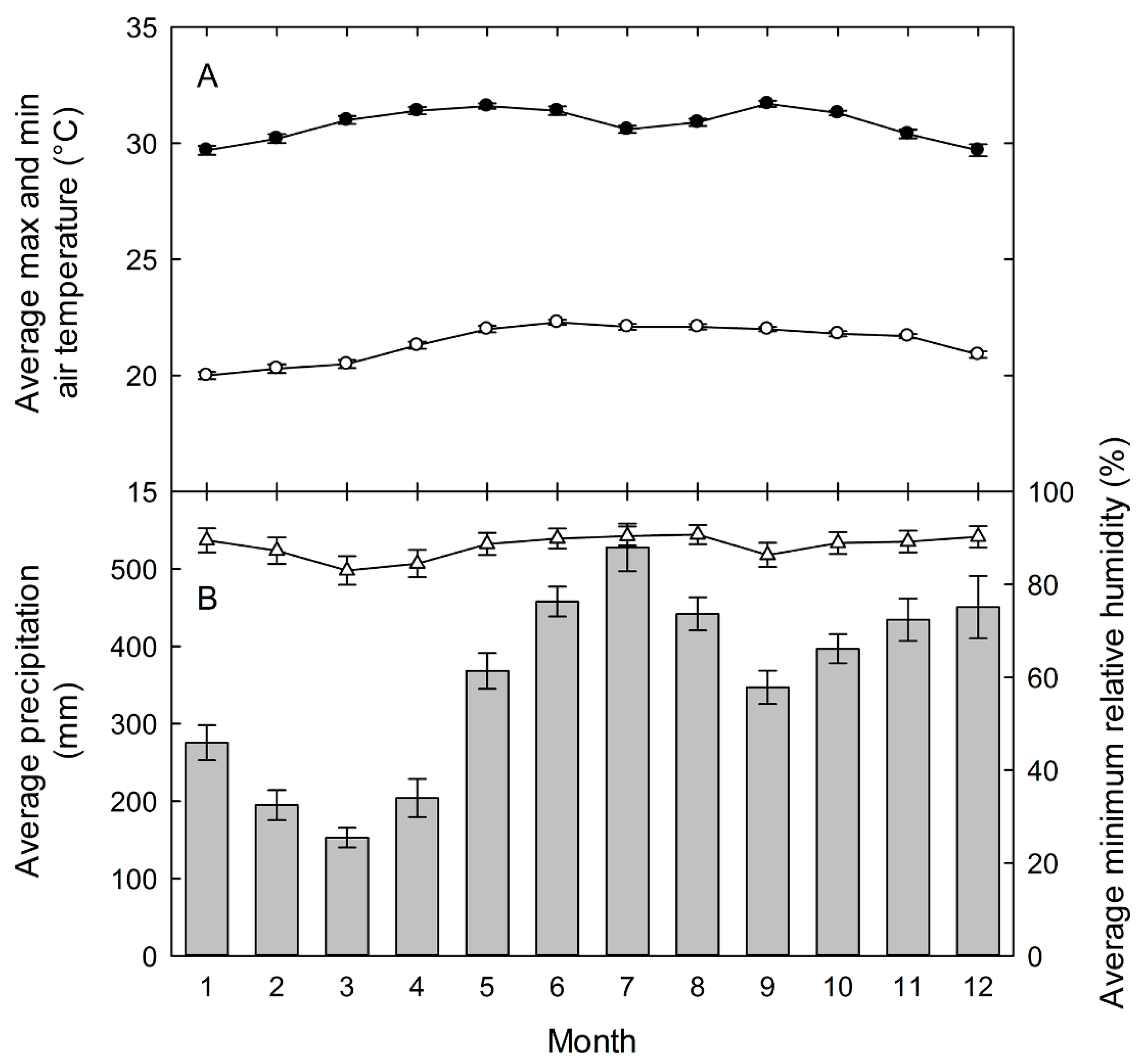
Field studies were carried out at the La Selva Biological Station from 2000 to 2009. La Selva is a 1500-hectare reserve of premontane wet forest in the Atlantic lowlands of Costa Rica (10°28′N, 83°59′W). The forest crown varies from 30 to 55 m in height with a closed canopy. The research station has a mean annual rainfall of 4244 mm (1958–2004), with a mean monthly rainfall above 300 mm from May through December (Figure 1). There are peaks of precipitation above 400 mm mo-1 in June–August and November–December, and a drier period from January to April. Even in the driest period of February and March, however, rainfall averages are above 150 mm each month. Air temperature is very stable annually, and the daily variation ranges from an observed maximum monthly mean of 31.7 ± 0.1 °C to a minimum of 20.0 ± 0.2 °C (Figure 1). The microclimatic conditions during measurements were within normal ranges for the dates of the study.
2.2. Mobile Sensing Platform
The NIMS RD system consists of a fixed cableway infrastructure, mounting hardware that is supported by this fixed cable, an auxiliary cable system which moves a shuttle along the fixed cableway, and the computer-controlled actuation module that contains and controls the drive motors for the auxiliary cables simultaneously with other data-collection features [37]. NIMS RD was developed for and has been applied to a range of environmental sensing applications including terrestrial, aquatic, and contaminant observation and management. In this application, the NIMS RD cableway was attached at one end to an anchored but repositionable step ladder in a well-maintained, regularly mowed clearing of only short grass surrounding the research facility buildings, about 5 m from a primary forest edge, and at the other end to a 5 cm-wide nylon strap secured around the trunks of two trees to obtain a repositionable terminus between the trees at about 35 m into the forest perpendicular to the edge (Figure 2).
Three transects into the forest which were approximately 8 m apart and were established as replicates and were run successively during the rainy season from the 9 to 13 September 2006. For each transect, a run consisted of the movement of the shuttle by NIMS RD in 1 m increments from a well-maintained clearing into the forest. The edge of the forest was abrupt and dense with vegetation that needed to be partially cleared to allow the shuttle to enter the forest, typical of an older, “sealed” forest edge [38]. Thus, the visual edge of the forest was distinct and the transition from the clearing to the forest was measurable to 10 cm. The shuttle was paused for 30 s at each location in a transect for the equilibration of the sensors and then moved to the next position. When the shuttle reached the forest end of the transect, the shuttle was returned directly to the clearing. Each transect was continuously measured for a minimum of 25 h and each run took about 30 min to complete. The shuttle was maintained at an average of 2.1 ± 0.3 m above the ground (n = 105 measured points), with the end points being the highest off the ground at about 2.6 m.
Transects varied in length and position relative to the forest edge (Table 1). A total of 84.9 h of shuttle operation occurred over three days with the data collected approximately every minute. Data collection failures for the shuttle occurred during the first transect after 15:45 h on the first day to 06:15 h the next day for the upward and downward facing solar radiometers and for the silicon pyranometer and quantum sensor, affecting the number of data points collected (Table 1). Sensors on the support structure in the clearing failed for the first transect on the second day of data collection from about midnight. No failures of data collection occurred for the two other transect runs.
Shuttle sensors included an aspirated radiation shield containing air temperature and relative humidity sensors (HM1500LF, Humirel, Chandler, AZ, USA), a silicon pyranometer for solar energy (400–1100 nm; LI-200, LI-COR, Lincoln, NE, USA), a silicon quantum sensor for photosynthetically active radiation (400–700 nm PPF; LI-COR LI-190), and a four-component net radiometer: upward and downward facing solar (305 to 2800 nm) and infrared (5000 to 50,000 nm) radiometers (CNR1, Kipp and Zonen Bohemia, NY, USA). From the four-component radiometer, derived values of net shortwave (solar) radiation, net IR (terrestrial) radiation, effective surface temperature, and effective canopy/sky temperature were calculated using the manufacturer’s equations. Data from all sensors were recorded by a datalogger (CR23X, Campbell Scientific, Logan, UT, USA) every 5 s and were downloaded to a computer at the end of each run. The datalogger was time-synchronized with the computer controlling NIMS RD movement. An additional datalogger (CR21X, Campbell Scientific, Logan, UT, USA) was placed on the NIMS RD support structure in the clearing, was time-synchronized with the NIMS RD controller, and collected air temperature, relative humidity, and solar energy every 5 s using identical instrumentation as was on the shuttle.
2.3. Data Analysis
As a first-order approximation, it was expected that the influence of the forest edge on the penetration of a microclimatic variable into or out of the forest, the depth of influence (DOI) would resemble a diffusion process, an exponential rise to a maximum or decay to a minimum, rather than a linear change at the edge. This magnitude and distance of edge influence [5] can be modeled with optimization performed in R, a freely available language and environment for statistical computing and graphics (R Development Core Team, 2006; www.cran.r-project.org; accessed on 13 December 2018). Specifically, data for each run of a transect were modeled as a two-part, piece-wise regression to estimate the point of inflection of two polynomials (one outside the edge and one inside the forest) and thus estimate the location of the forest edge, as measured by the specific sensor. The distance of this point of inflection from the visual forest edge was thus our measure of the DOI of the measured variable [3]. Four methods for fitting piece-wise regressions were tested, using either first- or second-order polynomials, used to generate a B-spline fit of the data with a single internal breakpoint (“knot”) that defined the junction of two the splines. The residuals of the knot location were then optimized using either a linear regression that minimized the sum of squares residuals or a quantile regression which was used to reduce the effect of outliers in the data. Normal quantile–quantile (Q–Q) plots were generated for each transect for visualizing the goodness of fit.
3. Results
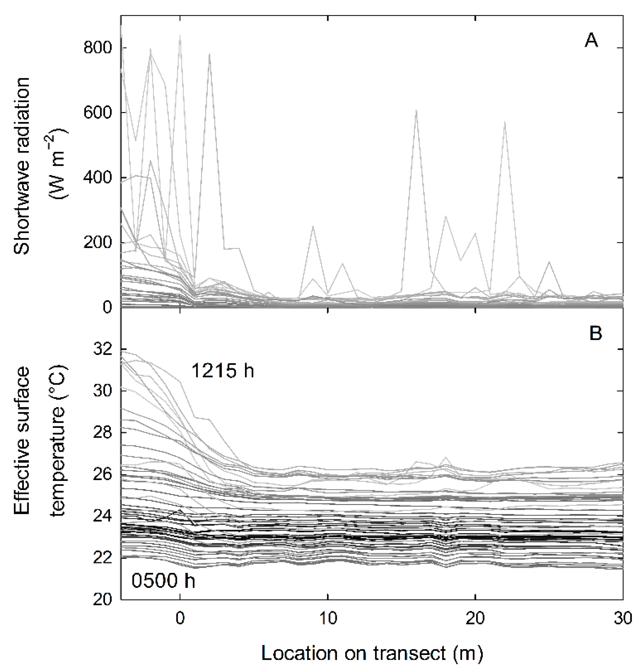
Instantaneous values of some micrometeorological sensors varied greatly with the time of day, the random effects of clouds, and gaps within the canopy (e.g., shortwave radiation sensors; Figure 3A). Other micrometeorological sensors and derived values from those sensors were more stable with respect to clouds and gaps (e.g., air temperature, relative humidity, effective surface temperature; Figure 3B).
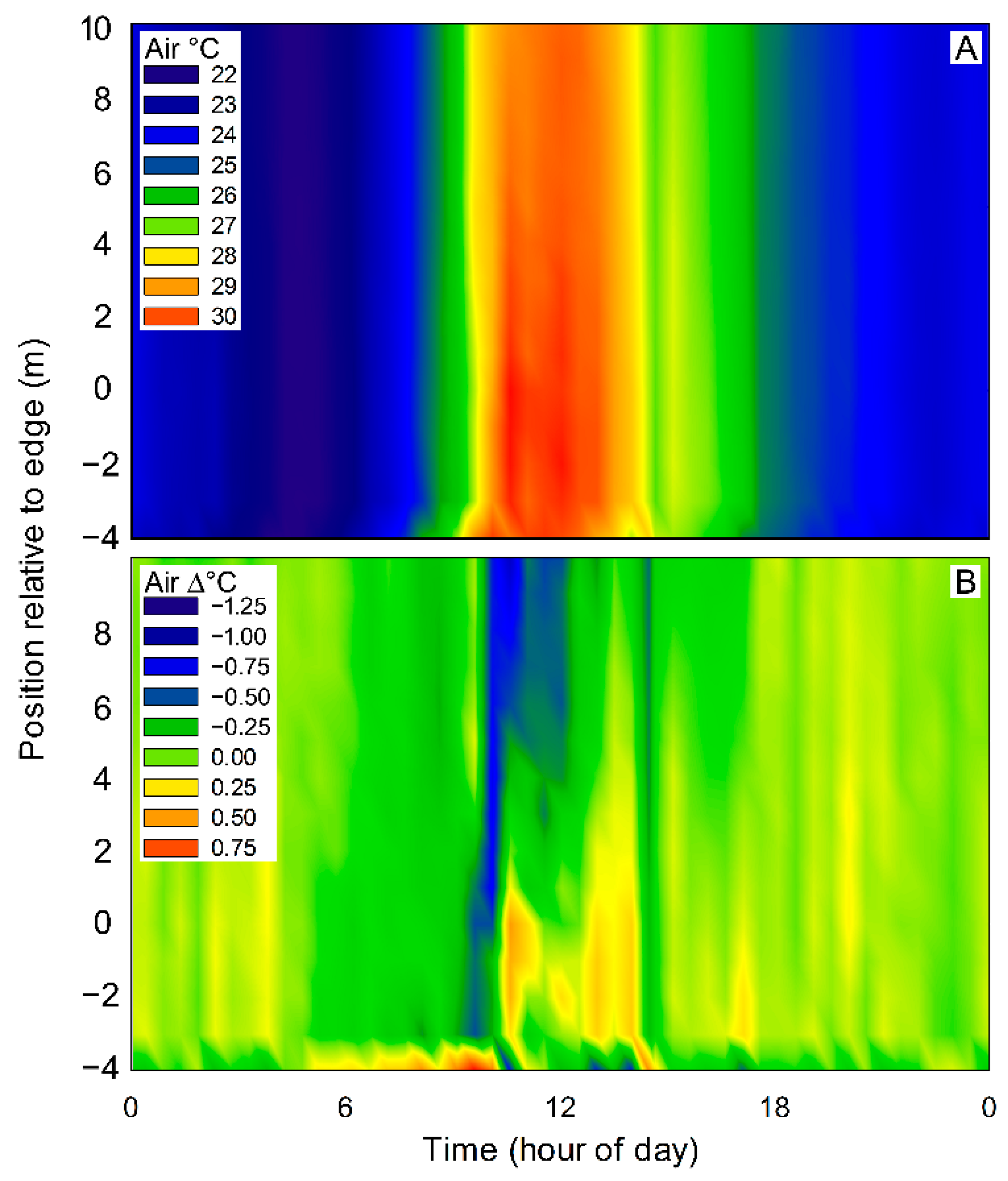
Nevertheless, the forest edge seemed apparent during at least parts of the day, by all sensors. For example, the average air temperature from 06:00 h to 16:00 h was significantly higher between the clearing at 4 m from the edge (29.46 ± 0.32 °C; mean ± S.E; n = 23) and 10 m into the forest (27.13 ± 0.39 °C; t-test; p < 0.001); however, from 17:00 h to 05:00 h, the next day, average air temperatures were not significantly different and differed between the two locations by only 0.04 °C (p = 0.898).
Continuous measurements of air temperature in the clearing and into the forest indicated that the daily variation in air temperature exceeded the maximum difference between the two areas (Figure 4A,B).
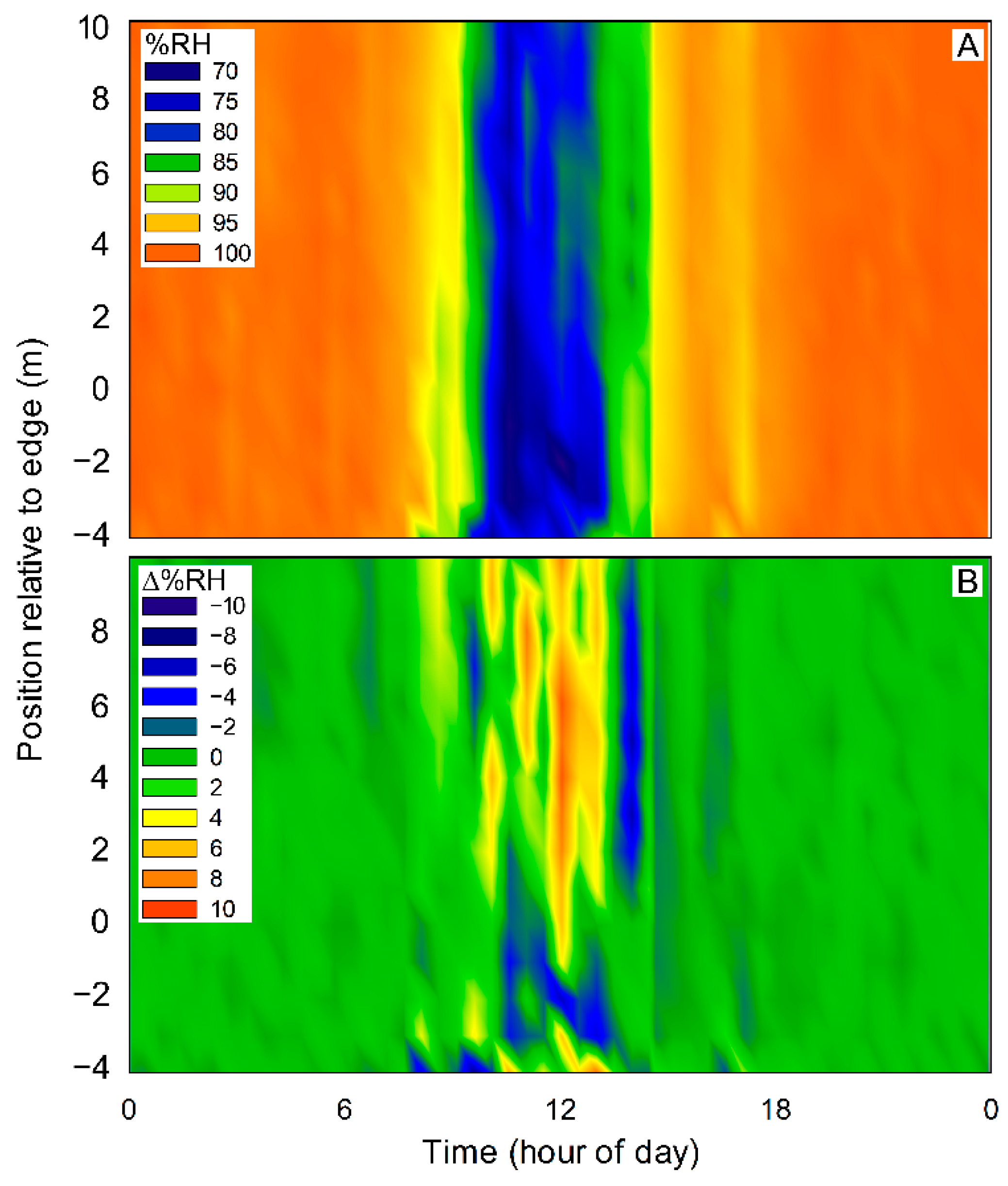
Relative humidity from 06:00 h to 16:00 h was significantly lower in the clearing at 4 m from the edge (69.86 ± 1.39%) compared to 10 m into the forest (88.02 ± 1.30%; t-test; p < 0.001). The significant difference continued in the evening, from 17:00 h to 05:00 h the next day, although the relative humidity in the forest in the night averaged at nearly 100% and the difference between the two locations was of only 6.3%, possibly exceeding the sensitivity of the sensor (t-test; p < 0.001; Figure 5A,B).
At sunrise, when the support structure station and shuttle pyranometers first detected shortwave radiation in the clearing (at about 06:25 h), none of the microclimatic variables measured on the shuttle differed significantly across the forest edge except for those involving the downward-facing IR sensor: the derived measurement of effective surface temperature, net IR and net radiation. For example, on the second transect at 06:17 h, the downward-facing IR sensor measured an average of 421.57 ± 1.24 W m−2 (mean ± SD, n = 6) in the clearing and 420.55 ± 0.71 W m−2 (n = 29) under the canopy (p < 0.008; t-test). This resulted in an average Effective Surface Temperature difference between the clearing and the forest floor of about 0.2 °C, after which the clearing temperature increased to a maximum of 6.4 °C at 08:45 h above the forest interior and then decreased to a minimum of 0.01 °C at 04:45 h the next morning. The upward-facing IR sensor was higher between the clearing and under the canopy only for the measurements farthest from the forest edge (data not shown).
Throughout the day, under the canopy, the effective canopy temperature was closely correlated to the air temperature measured under the canopy (slope of 1.05; r2 = 0.991) and in the clearing (slope of 0.97; r2 = 0.976). The silicon pyranometer and quantum sensors were also closely related to the upward facing shortwave sensor on the net radiometer. The largest differences in average microclimatic measurements between the clearing and in the understory occurred during midday (Table 2). Maximum differences between such average measurements varied considerably with the micrometeorological sensor type (Table 2), however, these were not always correlated with the accuracy of estimates of the forest edge (Table 3). For example, the small maximum differences in air temperature between the clearing and in the understory were reflected in the inaccurate average estimates of the forest edge (an average of 10.4 ± 2.8 m into the forest; n = 3 transects), for that measurement while the similarly small maximum differences in downward-facing infrared radiation were associated with more consistently accurate average edge estimates (1.4 ± 0.6 m).
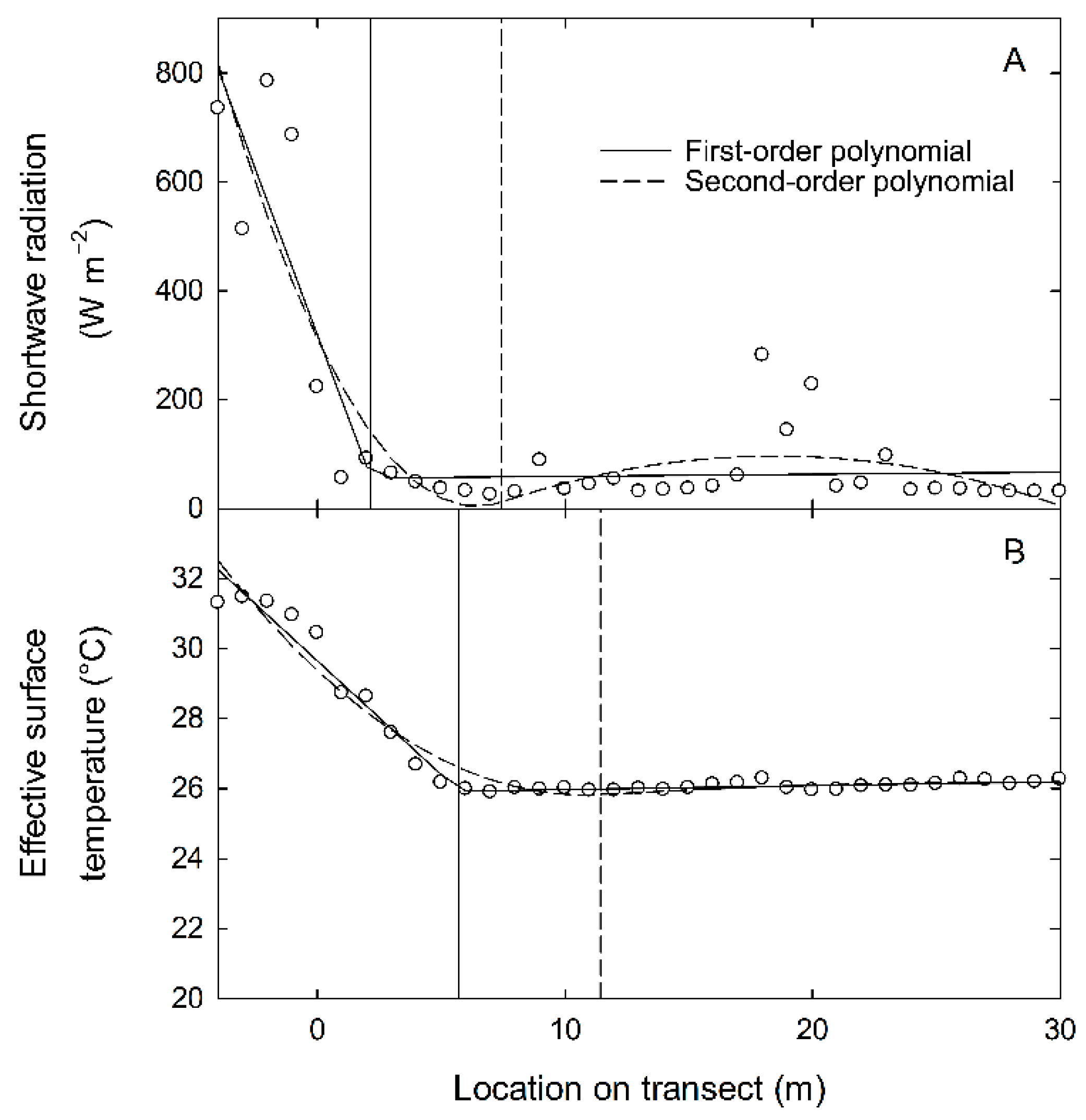
Locations of the estimated forest edge using piece-wise linear regressions were conducted for all transects and times, although values during the evening often resulted in poor estimates due to little or no differences across the transects. Using mid-day data for the shortwave radiation sensor, which is sensitive to the random effects of clouds and gaps within the canopy, the estimated forest edge was close to the visual edge using the first-order polynomial and either linear or quantile fits (quantile fits not shown, Figure 6A). A comparison to the derived sensor value of effective surface temperature, which is less sensitive, shows that the location of the estimated forest edge was not as good (Figure 6B). Using a second-order polynomial fit resulted in estimates that deviated even more greatly from the visual edge (dashed lines, Figure 6A,B).
The estimated location of the forest edge did not differ greatly between the linear regression and the quantile regression for the radiation sensors. For example, for transect #3 between 06:00 and 16:00 h, the maximum average difference between forest edge estimates between the two methods occurred for the downward facing IR sensor with a 2.3 ± 0.6 m difference between them (n = 24; p = 0.16; paired t-test); the minimum average difference between forest edge location estimates for this transect was for the net IR measurement at 0.07 ± 0.18 m.
Estimated daytime (06:00 h to 17:00 h) locations of the forest edge were primarily in the forest, relative to the visible edge, depending on the sensor used (Table 3). The sensors or derived sensor values that were closest to the visible the edge were either upward-facing shortwave sensor-based or downward-facing longwave sensor-based. Averaged among the transects, the sensor that estimated the forest edge the most closely during these hours was the upward-facing pyranometer (within 0.6 m), followed by the derived measurement of net IR radiation (within 0.7 m) and then the downward-facing infrared radiometer (within 1.5 m). Air temperature was the least similar measurement of the forest edge at 10.4 m into the forest and relative humidity was second with an estimated edge at 9.8 m into the forest (Table 3).
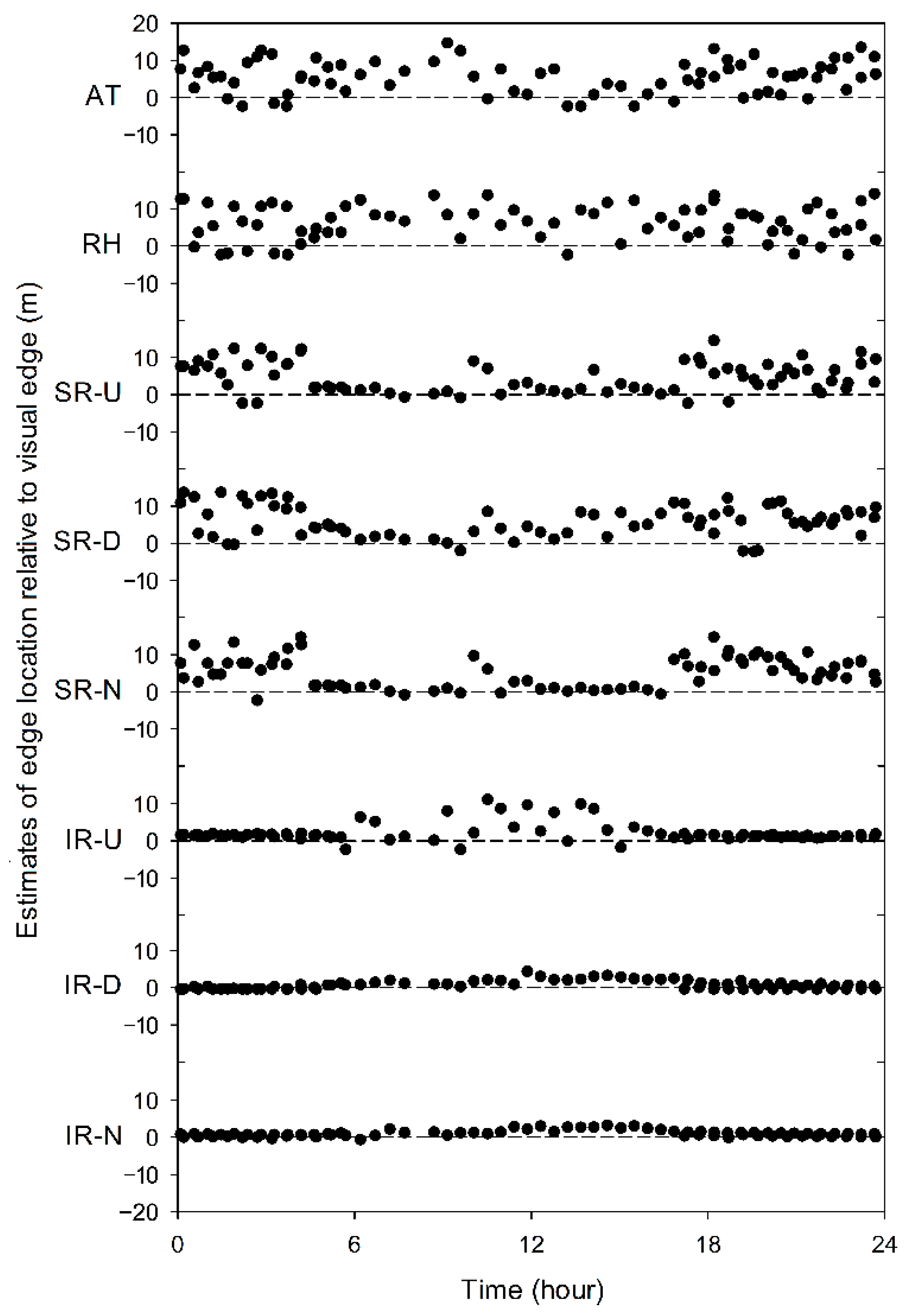
Instantaneous estimates of the forest edge relative to the visual edge varied with time and measurement type. For example, air temperature-based estimates of the forest edge on transect 2 were almost entirely in the interior of the forest and had a large inter-estimate variation (Figure 7; AT). Conversely, infrared measurements tended to have less variation and net infrared radiation, which consistently estimated the forest edge within 1 m (Figure 7; compare AT with IR). Shortwave radiation was better at estimating the edge during sunlit hours, with net shortwave radiation consistently providing estimates closer to the visual edge than either upward or downward facing shortwave radiation measurements alone (Figure 7; SR).
4. Discussion
The deployment of a mobile sensing platform to measure the fine-scale changes in microclimate conditions across a forest allowed the system to collect microclimate measurements every 1 m along three approximately 30 m transects for 24 h each. Measurements at each transect were made on consecutive days and were not collected simultaneously. Such synchronization was traded for the ability to measure in many locations with the same high-resolution sensors. Nevertheless, the flexibility of the system makes it easy to vary the spacing, timing, and duration for other sensor packages, purposes, or locations. Establishing spatially adjacent sampling units enabled the collection of the lattice (two-dimensional) data for more sophisticated statistical methods to characterize boundaries [8].
We found that a simple, first-order polynomial to quantify and describe the forest edge fit the data better than a higher-order polynomial, similar to previous studies using piece-wise regressions across edges [37], and that the linear and quantile regressions produced similar results. We did not encounter convergence problems when fitting, except for measurements of zero shortwave (solar) radiation at night, most likely because of the limited quantity of data available for the fit per sampling run and the relative homogeneity of the interior forest for the measurements conducted.
Our data indicate that reliable forest edge estimation, based on distance from the visually obvious and abrupt forest edge, can be made during the daytime with shortwave radiation sensors, similar to other studies [29]. We found that edge location estimates based on net shortwave radiation had less difference from the visual edge, most likely because net measurements reduce the large variation in solar radiation that can occur due to atmospheric conditions. The aspect of the forest edge face would necessarily affect solar radiation measurements with the time of day and our single-aspect edge measurements could potentially be significantly different for differently facing edges. Edge estimates made throughout the day with downward facing or net infrared radiation sensors were more consistent and closer to the visual edge than any other measurement. Transforming the infrared radiation measured from W m−2 into effective temperature in °C did not change the edge estimates but does allow for the use of more intuitive units and possible comparison to other studies that have used soil temperatures for edge effect determination [21,29]. Indeed, a review of 76 studies concerning forest edges indicates that the use of soil temperatures resulted in less variation of edge estimates into the forest than other standard microclimatic measurements [1].
A large number of descriptive studies have researched how microclimate changes across sharp transition zones exist in the literature [1,9], and recently, more attention has been focused on remote sensing and modeling edges for more quantifiable estimates of their effects [5,30,33,34,37]. Indeed, new methods, for example, of employing wide-view infrared cameras for the near-continuous monitoring of forest conditions to correlate with remote sensing and carbon flux measurements can similarly characterize the influence of sub-daily and fine-scale fluctuations of micrometeorological parameters [39]. However, the comparison of remote sensing products with in situ measurements is often necessarily limited to the specific sites with the highest degree of homogeneity in order to minimize the effect of the scale mismatch [40]. Thus, fine-scale temporal dynamics of microclimate have been mostly ignored in favor of larger time-scale measurements and or remote sensing models (air temperature, relative humidity, and light being the most common) such as values recorded daily at noon [26,41], for restricted hours of the day [42,43], or as summarized by daily averages, maxima and minima [10,44]. Exposing species distributions in areas of small-scale climatic variability, like forest understories, requires fine resolution climate data as can be collected with systems as the one presented in this study, particularly for examining temporary “holdouts” and microrefugia [7].
5. Conclusions
Our research contributes to the relatively small number of studies that have directly measured diurnal temporal and spatial patterns of microclimate variation [9] and fewer still have looked at these patterns across continuous spatial gradients rather than at a few sites located at the forest edge and interior. Our method of using a mobile platform to carry a sensor payload across a forest edge enables repeated, high-resolution measurements of gradients of microclimate. Our approach combined with using a simple, piece-wise regression lends itself to the rigorous depth of influence estimates that have been called for to understand the variability of responses of microclimate to forest edges [9].
Author Contributions
E.A.G. and P.W.R. jointly conceived and designed the research protocols using a NIMS-RD system developed by W.J.K., E.Y. and Y.L. Installation and operation of the NIMS-RD at the field site were made by E.A.G., E.Y., Y.L. and P.W.R., M.H. and E.A.G. analyzed data. E.A.G. and P.W.R. wrote the first draft of the manuscript and all authors reviewed the text and made edits. All authors have read and agreed to the published version of the manuscript.
Funding
This research was supported by the U.S. National Science Foundation under Grants ANI-00331481 and CCR-0120778.
Institutional Review Board Statement
This study did not involve humans or animals.
Informed Consent Statement
This study did not involve humans.
Data Availability Statement
Not applicable.
Acknowledgments
We would also like to thank staff members of the La Selva Biological Research Station who provided critical assistance and permitting to make this research possible.
Conflicts of Interest
The authors declare no conflict of interest. There were no sponsors that had a role in the design of the study; in the collection, analyses, or interpretation of data; in the writing of the manuscript, and in the decision to publish the results.
References
- Schmidt, M.; Jochheim, H.; Kersebaum, K.-C.; Lischeid, G.; Nende, L.C. Gradients of microclimate, carbon and nitrogen in transition zones of fragmented landscapes—A review. Agric. For. Meteorol. 2017, 232, 659–671. [Google Scholar] [CrossRef] [Green Version]
- Jucker, T.; Hardwick, S.R.; Both, S.; Elias, D.M.; Ewers, R.M.; Milodowski, D.T.; Coomes, D.A. Canopy structure and topography jointly constrain the microclimate of human-modified tropical landscapes. Glob. Chang. Biol. 2018, 24, 5243–5258. [Google Scholar] [CrossRef] [Green Version]
- Jucker, T.; Jackson, T.D.; Zellweger, F.; Swinfield, T.; Gregory, N.; Williamson, J.; Slade, E.M.; Phillips, J.W.; Bittencourt, P.R.; Blonder, B.; et al. A research agenda for microclimate ecology in human-modified tropical forests. Front. For. Glob. Chang. 2020, 2, 92. [Google Scholar] [CrossRef]
- Murcia, C. Edge effects in fragmented forests: Implications for conservation. Trends Ecol. Evol. 1995, 10, 58–62. [Google Scholar] [CrossRef]
- Harper, K.A.; Macdonald, S.E.; Burton, P.J.; Chen, J.; Brosofske, K.D.; Saunders, S.C.; Euskirchen, E.S.; Roberts, D.A.R.; Jaiteh, M.S.; Esseen, P.A. Edge influence on forest structure and composition in fragmented landscapes. Conserv. Biol. 2005, 19, 768–782. [Google Scholar] [CrossRef]
- Laurance, W.F. Do edge effects occur over large spatial scales? Trends Ecol. Evol. 2000, 15, 134–135. [Google Scholar] [CrossRef]
- Lembrechts, J.J.; Nijs, I.; Lenoir, J. Incorporating microclimate into species distribution models. Ecography 2019, 42, 1267–1279. [Google Scholar] [CrossRef]
- Fagan, W.F.; Fortin, M.-J.; Soykan, C. Integrating edge detection and dynamic modeling in quantitative analyses of ecological boundaries. BioScience 2003, 53, 730–738. [Google Scholar] [CrossRef] [Green Version]
- Ries, L.; Murphy, S.M.; Wimp, G.M.; Fletcher, R.J. Closing persistent gaps in knowledge about edge ecology. Curr. Lands Ecol. Rep. 2017, 2, 30–41. [Google Scholar] [CrossRef] [Green Version]
- Chen, J.; Franklin, J.F.; Spies, T.A. Growing season microclimatic gradients from clearcut edges into old growth Douglas-fir forest. Ecol. Appl. 1995, 5, 74–86. [Google Scholar] [CrossRef]
- Meiners, S.J.; Pickett, S.T.A.; Handel, S.N. Probability of tree seedling establishment changes across a forest-old field edge gradient. Am. J. Bot. 2002, 89, 466–471. [Google Scholar] [CrossRef] [Green Version]
- Benitez-Malvido, J.; Lemus-Albor, A. The seedling community of tropical rain forest edges and its interaction with herbivores and pathogens. Biotropica 2005, 37, 301–313. [Google Scholar] [CrossRef]
- Wirth, R.; Meyer, S.T.; Leal, I.R.; Tabarelli, M. Plant herbivore interactions at the forest edge. Prog. Bot. 2008, 69, 423–448. [Google Scholar]
- Yahner, R.H. Changes in wildlife communities near edges. Conserv. Biol. 1988, 2, 333–339. [Google Scholar] [CrossRef]
- Kareiva, P. Habitat fragmentation and the stability of predator-prey interactions. Nature 1987, 326, 388–390. [Google Scholar] [CrossRef]
- Fagan, W.E.; Cantrell, R.S.; Cosner, C. How habitat edges change species interactions. Am. Nat. 1999, 153, 165–182. [Google Scholar] [CrossRef] [PubMed]
- Foggo, A.; Ozanne, C.M.P.; Speight, M.R.; Hambler, C. Edge effects and tropical forest canopy invertebrates. Plant Ecol. 2001, 153, 347–359. [Google Scholar] [CrossRef]
- Asquith, N.M.; Mejia-Chang, M. Mammals, edge effects, and the loss of tropical forest diversity. Ecology 2005, 86, 379–390. [Google Scholar] [CrossRef] [Green Version]
- Ewers, R.M.; Boyle, M.J.; Gleave, R.A.; Plowman, N.S.; Benedick, S.; Bernard, H.; Turner, E.C. Logging cuts the functional importance of invertebrates in tropical rainforest. Nat. Commun. 2015, 6, 6836. [Google Scholar] [CrossRef]
- Chen, J.Q.; Saunders, S.C.; Crow, T.R.; Naiman, R.J.; Brosofske, K.D.; Mroz, G.D.; Brookshire, B.L.; Franklin, J.F. Microclimate in forest ecosystem and landscape ecology. BioScience 1999, 49, 288–297. [Google Scholar] [CrossRef] [Green Version]
- Dodonov, P.; Menezes, G.S.C.; Caitano, B.; Cazetta, E.; Mielke, M.S. Air and soil temperature across fire-created edges in a Neotropical rainforest. Agric. For. Meteorol. 2019, 276, 107606. [Google Scholar] [CrossRef]
- Menezes, G.S.C.; Cazetta, E.; Dodonov, P. Vegetation structure across fire edges in a Neotropical rain forest. For. Ecol. Manag. 2019, 453, 117587. [Google Scholar] [CrossRef]
- Grimmond, C.S.B.; Robeson, S.M.; Schoof, J.T. Spatial variability of micro-climatic conditions within a mid-latitude deciduous forest. Clim. Res. 2000, 15, 137–149. [Google Scholar] [CrossRef]
- Camargo, J.C.L.; Kapos, V. Complex edge effects on soil moisture and microclimate in central Amazonian forest. J. Trop. Ecol. 1995, 11, 205–221. [Google Scholar] [CrossRef]
- Kapos, V.; Wandelli, E.E.; Camargo, J.L.; Ganade, G. Edge-related changes in environment and plant responses due to forest fragmentation in central Amazonia. In Tropical Forest Remnants: Ecology, Management, and Conservation of Fragmented Communities; Laurance, W.F., Bierregaard, R.O., Eds.; University of Chicago Press: Chicago, IL, USA, 1997; pp. 33–44. [Google Scholar]
- Williams-Linera, G.; Dominguez-Gastelu, V.; Garcia-Zurita, M.E. Microenvironment and floristics of different edges in a fragmented tropical rainforest. Conserv. Biol. 1998, 12, 1091–1102. [Google Scholar] [CrossRef]
- Dignan, P.; Bren, L. Modelling light penetration edge effects for stream buffer design in mountain ash forest in southeastern. Aust. For. Ecol. Manag. 2003, 175, 95–106. [Google Scholar] [CrossRef]
- Saunders, D.A.; Hobbs, R.J.; Margules, C.R. Biological consequences of ecosystem fragmentation: A review. Conserv. Biol. 1991, 5, 18–32. [Google Scholar] [CrossRef]
- Li, Y.; Kang, W.; Han, Y.; Song, Y. Spatial and temporal patterns of microclimates at an urban forest edge and their management implications. Environ. Monit. Assess. 2018, 190, 93. [Google Scholar] [CrossRef] [PubMed]
- Fortin, M.-J.; Olson, R.J.; Ferson, S.; Iverson, L.; Hunsaker, C.; Edwards, G.; Levine, D.; Butera, K.; Klemas, V. Issues related to the detection of boundaries. Land Ecol. 2000, 15, 453–466. [Google Scholar] [CrossRef]
- Saunders, S.C.; Chen, J.Q.; Drummer, T.D.; Crow, T.R. Modeling temperature gradients across edges over time in a managed landscape. For. Ecol. Manag. 1999, 117, 17–31. [Google Scholar] [CrossRef]
- Newmark, W.D. Tanzanian forest edge microclimatic gradients: Dynamic patterns. Biotropica 2001, 33, 2–11. [Google Scholar] [CrossRef]
- Bramer, I.; Anderson, B.J.; Bennie, J.; Bladon, A.J.; De Frenne, P.; Hemming, D.; Gillingham, P.K. Advances in monitoring and modelling climate at ecologically relevant scales. Adv. Ecol. Res. 2018, 58, 101–161. [Google Scholar] [CrossRef]
- Wild, J.; Kopecký, M.; Macek, M.; Šanda, M.; Jankovec, J.; Haase, T. Climate at ecologically relevant scales: A new temperature and soil moisture logger for long-term microclimate measurement. Agric. For. Meteorol. 2019, 268, 40–47. [Google Scholar] [CrossRef]
- Zellweger, F.; Frenne, P.; De Lenoir, J.; Rocchini, D.; Coomes, D. Advances in microclimate ecology arising from remote sensing. Trends Ecol. Evol. 2019, 34, 327–341. [Google Scholar] [CrossRef] [Green Version]
- Toms, J.D.; Lesperance, M.L. Piecewise regression: A tool for identifying ecological thresholds. Ecology 2003, 84, 2034–2041. [Google Scholar] [CrossRef]
- Jordan, B.L.; Batalin, M.A.; Kaiser, W.J. NIMS RD: A Rapidly Deployable Cable Based Robot. ICRA’07. In Proceedings of the 2007 IEEE International Conference on Robotics and Automation, Roma, Italy, 10–14 April 2007. [Google Scholar]
- Restrepo, C.; Gomez, N.; Heredia, S. Anthropogenic edges, treefall gaps, and fruit–frugivore interactions in a neotropical montane forest. Ecology 1999, 80, 668–685. [Google Scholar]
- Kim, Y.; Still, C.J.; Hanson, C.V.; Kwon, H.; Greer, B.T.; Law, B.E. Canopy skin temperature variations in relation to climate, soil temperature, and carbon flux at a ponderosa pine forest in central Oregon. Agric. For. Meteorol. 2016, 226–227, 161–173. [Google Scholar] [CrossRef] [Green Version]
- Cescatti, A.; Marcolla, B.; Santhana Vannan, S.K.; Yun Pan, J.; Román, M.O.; Yang, X.; Ciais, P.; Cook, R.B.; Law, B.E.; Matteucci, G.; et al. Intercomparison of MODIS albedo retrievals and in situ measurements across the global FLUXNET network. Remote Sens. Environ. 2012, 121, 323–334. [Google Scholar] [CrossRef] [Green Version]
- Cadenasso, M.L.; Traynor, M.M.; Pickett, S.T.A. Functional location of forest edges: Gradients of multiple physical factors. Can. J. For. Res. 1997, 27, 774–782. [Google Scholar] [CrossRef]
- Davies-Colley, R.J.; Payne, G.W.; van Elswijk, M. Microclimate gradients across a forest edge. N. Z. J. Ecol. 2000, 24, 111–121. [Google Scholar]
- Gehlhausen, S.M.; Schwartz, M.W.; Augspurger, C.K. Vegetation and microclimatic edge effects in two mixed mesophytic forest fragments. Plant Ecol. 2000, 147, 21–35. [Google Scholar] [CrossRef]
- Chen, J.; Franklin, J.F.; Spies, T.A. Contrasting microclimates among clearcut, edge, and interior of old-growth Douglas-fir forest. Agric. For. Meteorol. 1993, 63, 219–237. [Google Scholar] [CrossRef]
Figure 1.
(A) Daily maximum (closed circles) and minimum (open circles) air temperatures; and (B) total monthly precipitation (vertical bars), and daily minimum relative humidity (open triangles) (B) for the La Selva Biological Station, Costa Rica. Values are the means ± standard errors for each month for data collected hourly from 1957 to 2003 for precipitation, from 1982 to 2003 for temperature, and from 1992 to 2003 for relative humidity.

Figure 2.
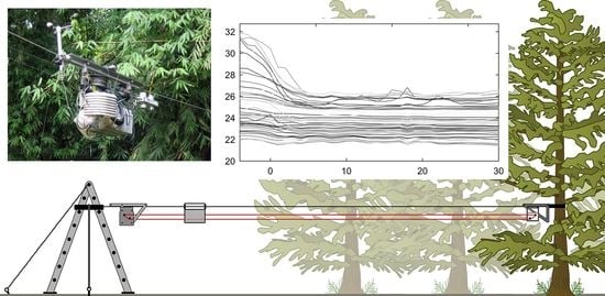
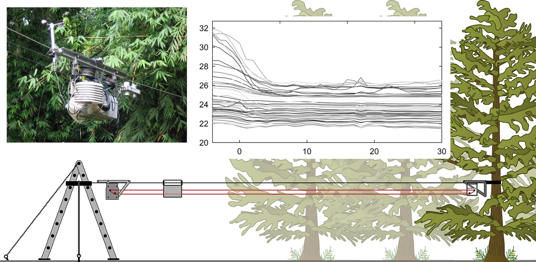
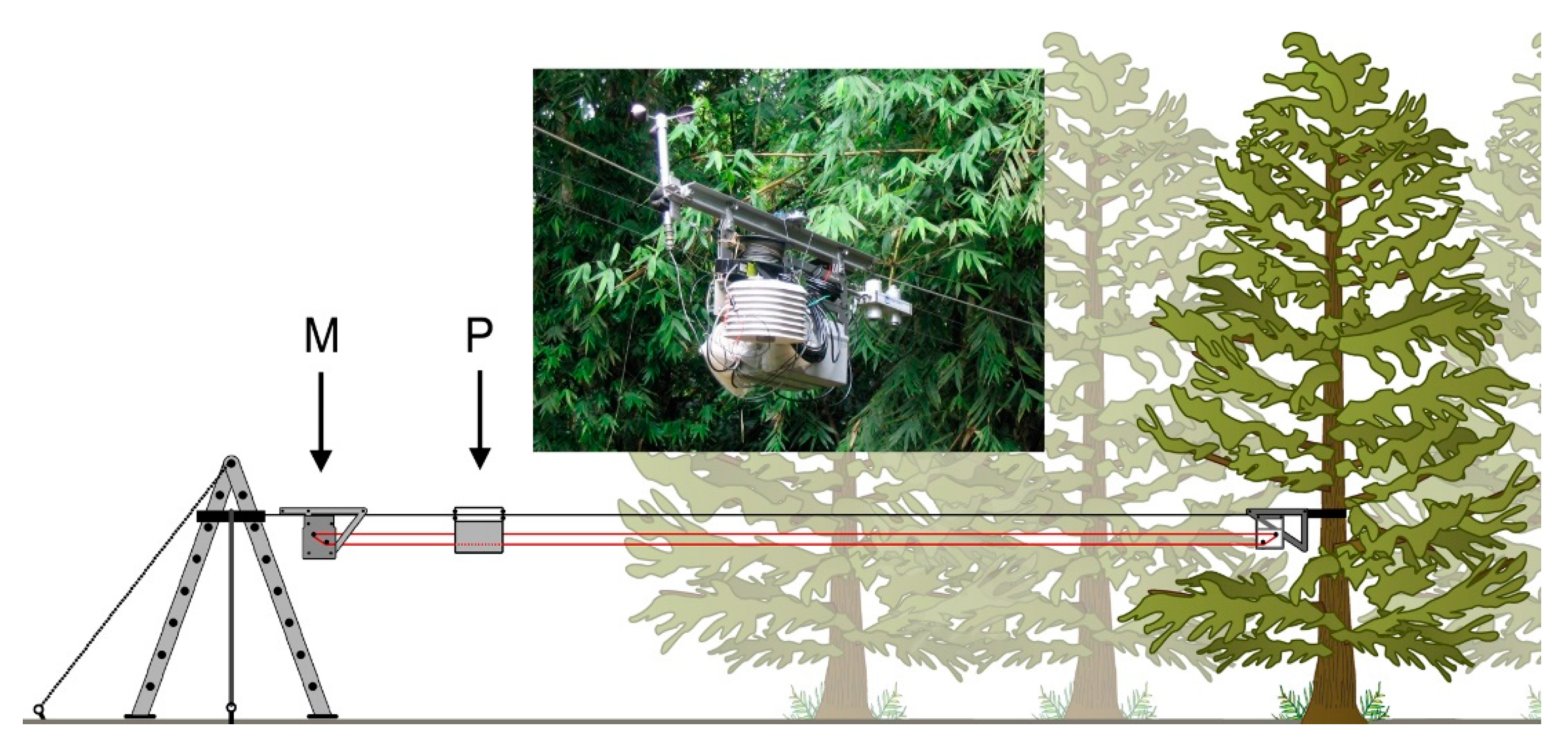
The NIMS RD system for measuring the influence of a forest edge on microclimate (not to scale). The horizontal cableway (top black line) is anchored in the clearing to a support structure (here, a repositionable step ladder) and in the forest to the trunk of a tree or between two trees by means of an adjustable strap. The payload (P) is composed of interchangeable micrometeorological sensors connected to an integrated datalogger. Control of the position of the payload is by a motor assembly (M), that moves a looped auxiliary drive cable (red line), similar in function to a continuous clothesline. Data and power are either transferred by cable festooned to the payload (not shown) or data are downloaded periodically to a portable computer and power is from batteries integrated into the payload. The inset shows the actual NIMS-RD unit.
Figure 2.
The NIMS RD system for measuring the influence of a forest edge on microclimate (not to scale). The horizontal cableway (top black line) is anchored in the clearing to a support structure (here, a repositionable step ladder) and in the forest to the trunk of a tree or between two trees by means of an adjustable strap. The payload (P) is composed of interchangeable micrometeorological sensors connected to an integrated datalogger. Control of the position of the payload is by a motor assembly (M), that moves a looped auxiliary drive cable (red line), similar in function to a continuous clothesline. Data and power are either transferred by cable festooned to the payload (not shown) or data are downloaded periodically to a portable computer and power is from batteries integrated into the payload. The inset shows the actual NIMS-RD unit.

Figure 3.
Examples of repeated measurements across the forest edge through a 24 h period on transect #3 for (A) shortwave radiation and (B) effective surface temperature. The different intensity of gray lines indicates the time at the beginning of separate runs (darkest is midnight, lightest is noon) and for (B), the hour of the topmost and bottom-most lines is indicated.

Figure 4.
Absolute air temperature (A) and that relative to the clearing (B) for transect #3. Distance into the forest is relative to the edge, which is located at zero.
Figure 4.
Absolute air temperature (A) and that relative to the clearing (B) for transect #3. Distance into the forest is relative to the edge, which is located at zero.

Figure 5.
Absolute relative humidity (A) and that relative to the clearing (B) for transect #3. Distance into the forest is relative to the edge, which is located at zero.
Figure 5.
Absolute relative humidity (A) and that relative to the clearing (B) for transect #3. Distance into the forest is relative to the edge, which is located at zero.

Figure 6.
Forest edge estimates based on first (solid) or second-order (dashed line) piecewise polynomials using a least squares regression fit. The forest edge estimate is the junction of the two splines and is indicated by a vertical line of the same type. The sensor values for shortwave radiation (A) and the derived values of effective surface temperature (B) were from transect #3 and taken during a run that began at 12:15 h.

Figure 7.
Example of forest edge estimates, based on the quantile regression fit for a first-order polynomial, relative to the visual edge over 24 h for transect #2 for selected microclimatic variables measured on the shuttle. Y axis units are a positive distance (m) into the forest and negative into the clearing relative to the edge (dashed lines). Microclimatic measurements are air temperature (AT); relative humidity (RH); solar radiation upwards (SR-U); solar radiation downwards (SR-D); net solar radiation (SR-N); infrared radiation upwards (IR-U); infrared radiation downwards (IR-D); and net infrared radiation (IR-N).


Table 1.
Lengths, locations and data collection information for each transect.
| Transect | Total Transect Length (m) | Relative Location of Base in Clearing from Forest Edge (m from Edge) | Number of Measurement Repetitions (“Runs”) in Approximately 24 h | Total Number of Data Points Collected per Sensor |
|---|---|---|---|---|
| 1 | 37 | −6 | 42 | 1065 |
| 2 | 27 | −6 | 77 | 1848 |
| 3 | 35 | −4 | 52 | 1820 |
Table 2.
Times of day for the maximum differences between the average clearing value (n = 4 or 6 per transect) and the average under the canopy value (n > 20) for selected microclimatic variables measured on the shuttle (excluding zero values), averaged among all three transects; values are means ± SD; n = 3.
| Variable | Time | In Clearing | Under Canopy |
|---|---|---|---|
| Air temperature (°C) | 11.8 ± 0.9 | 28.9 ± 1.0 | 27.7 ± 0.7 |
| Relative humidity (%) | 13.4 ± 1.9 | 79.2 ± 6.4 | 88.2 ± 5.7 |
| Solar radiation, upward-facing (W m−2) | 11.1 ± 0.6 | 558.5 ± 291.3 | 33.6 ± 25.1 |
| Solar radiation, downward-facing (W m−2) | 10.6 ± 0.8 | 51.7 ± 26.9 | 4.5 ± 2.9 |
| Net solar radiation (W m−2) | 11.1 ± 0.6 | 511.1 ± 268.2 | 29.6 ± 21.6 |
| IR radiation, upward-facing (W m−2) | 13.4 ± 8.8 | 434.8 ± 27.2 | 437.3 ± 15.2 |
| IR radiation, downward-facing (W m−2) | 12.3 ± 1.4 | 483.4 ± 15.5 | 448.1 ± 6.8 |
| Net IR radiation (W m−2) | 12.3 ± 1.4 | −25.4 ± 11.8 | 8.5 ± 3.4 |
Table 3.
Mean (±SE) daytime (06:00 h to 17:00 h) relative locations of the forest edge estimated by first-order, piece-wise linear regressions using quantile fits for selected microclimatic variables measured on the shuttle; positive values indicate a location into the forest from the visual edge and negative values indicate a location into the clearing.
| Variable | Relative Location of Edge (m) | ||
|---|---|---|---|
| Transect 1 (n = 16) | Transect 2 (n = 21) | Transect 3 (n = 24) | |
| Air temperature | 13.2 ± 1.5 | 7.6 ± 1.1 | 10.4 ± 1.5 |
| Relative humidity | 13.1 ± 2.0 | 7.7 ± 0.8 | 8.6 ± 1.5 |
| Solar radiation, upward-facing | −1.4 ± 0.4 | 2.9 ± 0.8 | 0.2 ± 0. 5 |
| Solar radiation, downward-facing | 7.0 ± 1.1 | 3.3 ± 0.8 | 1.3 ± 0.3 |
| Net solar radiation | 1.1 ± 2.1 | 7.2 ± 1.1 | −0.2 ± 0.5 |
| IR radiation, upward-facing | 6.9 ± 3.1 | 7.1 ± 1.0 | 1.4 ± 1.4 |
| IR radiation, downward-facing | 1.8 ± 0.2 | 1.8 ± 0.2 | 0.8 ± 0.2 |
| Net IR radiation | 0.6 ± 0.2 | 1.7 ± 0.2 | −0.2 ± 0.2 |
Publisher’s Note: MDPI stays neutral with regard to jurisdictional claims in published maps and institutional affiliations. |
© 2021 by the authors. Licensee MDPI, Basel, Switzerland. This article is an open access article distributed under the terms and conditions of the Creative Commons Attribution (CC BY) license (https://creativecommons.org/licenses/by/4.0/).
Share and Cite
MDPI and ACS Style
Graham, E.A.; Hansen, M.; Kaiser, W.J.; Lam, Y.; Yuen, E.; Rundel, P.W. Dynamic Microclimate Boundaries across a Sharp Tropical Rainforest–Clearing Edge. Remote Sens. 2021, 13, 1646. https://0-doi-org.brum.beds.ac.uk/10.3390/rs13091646
AMA Style
Graham EA, Hansen M, Kaiser WJ, Lam Y, Yuen E, Rundel PW. Dynamic Microclimate Boundaries across a Sharp Tropical Rainforest–Clearing Edge. Remote Sensing. 2021; 13(9):1646. https://0-doi-org.brum.beds.ac.uk/10.3390/rs13091646
Chicago/Turabian StyleGraham, Eric A., Mark Hansen, William J. Kaiser, Yeung Lam, Eric Yuen, and Philip W. Rundel. 2021. "Dynamic Microclimate Boundaries across a Sharp Tropical Rainforest–Clearing Edge" Remote Sensing 13, no. 9: 1646. https://0-doi-org.brum.beds.ac.uk/10.3390/rs13091646
Note that from the first issue of 2016, this journal uses article numbers instead of page numbers. See further details here.