1. Introduction
With the ability to unify features at different image levels, deep-learning networks have achieved great success in the remote sensing field. However, a deep-learning network’s performance mainly depends on (1) the size and variety of the training data and (2) the accuracy of the training labels. Compared to the former factor, errors in training labels are usually hard to identify and correct. Unlike the nature-image dataset in the computer-science field, noisy labels are more likely to occur in remote-sensed image datasets. First, the main reasons are that the land-cover and land-use type characteristics may vary depending on different times, locations and sensors. Identifying accurate labels requires specific background knowledge [
1]. Second, inconsistency of labels occurs when experts from different backgrounds make labels [
2]. Third, the historic land-cover/land-use maps are usually used in automatic-labeling processing. The unreliability of labels can be caused by the time mismatch between these historical maps and the images. Designing a framework to intensify deep-learning networks to reduce the impact of these erroneous samples is a much greater challenge.
The fundamental reason why the noisy-labeled samples can quickly impact the current deep networks is that, in a deep learning network, the network parameters are updated by samples with a high value in the loss function. Unfortunately, high-loss values can both be caused by correct samples with variate features and noisy-labeled samples. In the original network, there is no mechanism to distinguish these two types of samples. As a result, when the number of noisy-labeled samples increases, the network parameters are updated in the wrong direction by learning these incorrectly labeled samples. Therefore, adding a structure to help the deep-learning network distinguish noisy-labeled samples from correct samples is key to increasing the network’s robustness.
Recently, some attempts have been made to overcome this difficulty to distinguish the noisy-labeled samples. The strategy can be classified into two categories: (1) methods focused on labels and (2) methods focused on the loss function.
In the first category, there are three main types of methods: (1) the data-selection model, (2) the multiple-networks model and (3) the noise-transition-matrix model.
The first type is the data-selection model, which is to clean up the noisy labels by creating a mechanism. Learning the training samples step by step to clean up samples with a low-to-high loss value is one of the typical methods employed [
3]. These methods assume that the noisy-labeled samples usually show extremely high loss values compared to the samples with correct labels. Based on this assumption, the network can be first trained by the samples with a low-loss value; then the high-loss samples can be added step by step to the network and the network’s performance monitored at the same time. When the overall network loss is acceptable, the remaining high-loss samples are considered the errors. This assumption can hold when the variety of the samples is relatively low. However, a high-data variation over time or a satellite platform makes this strategy inappropriate. MORPH [
4] introduces the concept of deep-learning-network memory samples, which updates the initial set of samples containing noisy labels to the sample set of clean samples by self-transition learning. The data selection can also be improved by the higher-order topological information of the data. Based on this idea, the TopoFilter [
5] is proposed as a new noise-label-filtering method to detect clean-labeled samples. Semisupervised methods can also help to select the clean data. DivideMix [
6] combines semisupervised learning with label-noise learning by leveraging two-component and one-dimensional Gaussian mixture models to distinguish the clean samples from the noisy samples to train the model with the semisupervised methods. RoCL [
7] adopts a two-stage learning strategy to supervise the training of selected clean samples. Then semisupervised learning is performed to generate pseudo-labels by relabeling the noisy samples with the trained network.
Another clean-up strategy can also be created by two networks with different structures [
8]. The idea behind this strategy is that a different structure shows a different capacity to avoid different types of noise. They can cooperate to improve the ability to reduce the influence of noisy-labeled samples. In this method, the key task is to create specific rules to distinguish the erroneous samples. Once the rules fail in one step during the training section, the network may refuse to learn from the remaining correct samples.
The noise-transition matrix is the third type of method in this category. In these models, a transition matrix or layer is added to the end of the network to provide a chance for each sample to transfer its label to others [
9,
10,
11]. The matrix tries to correct the noisy data by quantifying the probability from one class to another. Most of the existing noise-transfer-matrix methods rely on estimating the noisy-class posterior. Still, the estimation error in the noisy-class posterior leads to poor estimates of the transfer matrix. The accuracy of this transfer matrix depends on the estimation of how the noise data are distributed in different categories. Dual T [
12] solves this problem by using a partitioning paradigm to decompose the matrix into two estimated matrices for multiplication to avoid directly estimating the noisy class posterior. However, in remote-sensing-classification problems, sometimes obtaining these kinds of matrices in practice is still a challenge.
The second category method focuses on how to decrease the impact of noisy data by reducing the loss values during the training process. One way to achieve this goal is to modify the loss function. The basic idea is to design a robust loss function that suffers less impact from the erroneous samples. After comparing the mean absolute error (MAE), mean square error (MSE) and categorical cross-entropy (CCE) loss functions, Ghosh et al. (2017) found that the MAE loss function is more robust to noise in multiple classification tasks [
13]. Based on this finding, Zhang and Sabuncu (2018) provided a generalized cross-entropy (GCE) loss function, which combined the MAE function with CCE to achieve higher performance when erroneous data were included [
14]. Later, inspired by the symmetric KL-divergence, symmetric cross-entropy learning (SL) [
15] was proposed, boosting cross-entropy (CE) symmetrically with a noise-robust counterpart, reverse cross-entropy (RCE). The SL approach simultaneously addresses both the insufficient learning and overfitting problem of CE in the presence of noisy data. The main drawback of these models is that the different types of noise in data labels are difficult to remove by one universal-loss function, which causes the low flexibility of the models. Moreover, the more complex the loss function, the more time is consumed during the training stage [
14].
This category’s other approach is to assign each training sample with a consistently updated weight during each learning iteration. The weighting process can help the model avoid noisy samples to achieve an accuracy equaling the mode trained with clean data [
16]. The critical issue in this category is how to calculate the weights for different samples. Many structures have been created to achieve this goal. For example, the multilayer perceptron (MLP) is used to estimate the weighting function [
17] and for the implicit calculation of the weighting factor [
18,
19]. All these models are designed and applied in image-sense classification tasks. To the best of the authors’ knowledge, there are no attempts to achieve this goal in the image-pixel classification task, especially in remote-sensing land-cover classification.
This article proposes a general network framework to prevent noisy-labeled data in remote-sensing image-classification tasks: the Weighted Loss Network (WLN). The WLN follows the idea of the loss-value weighting strategy in the second category mentioned above. We designed a sample weight-adjustment scheme in combination with the attention mechanism to evaluate each sample’s importance through the learning process. The experiments were performed on the remote-sensing-image public data set of the Inria Aerial Image Labeling Dataset and compared with the original classification-network method. This paper’s main contributions are summarized as follows: (1) we propose a general network framework that is robust for noisy-labeled training samples for remote-sensing image classification; (2) four commonly occurring types of label noise (an insufficient label, redundant label, missing label and incorrect label) are considered. The result shows the provided algorithm can maintain high accuracy and good generalization performance under different noise types.
3. Methodology
3.1. Study Workflow
In this paper, we designed a new end-to-end antinoise algorithm, the Weighted Loss Network (WLN), to assign weights to all training samples’ loss values and iteratively update these weights during the training process by improving the cross-entropy loss.
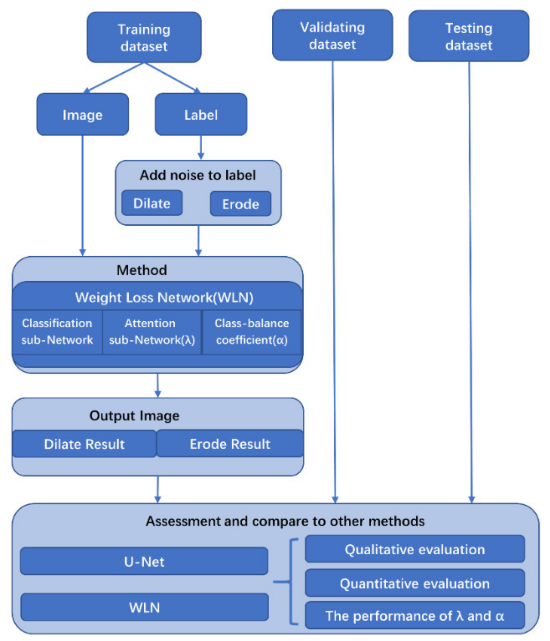
Figure 3 shows an overview of the workflow of this study.
As shown in
Figure 3, during training the noisy-labeled samples were added under 0%, 25%, 35%, 45% and 50% noise rates with three noise levels (kernel sizes of 9, 17 and 25) of dilation or erosion processing. The Weighted Loss Network is a universal antinoise framework with three components: (1) a classifier network (we use U-Net as the classifier in this study), (2) an attention subnetwork (λ), and (3) a class-balance part (
). The classifier network can be changed for other deep-learning-based networks depending on the different applications. To evaluate the performance of the WLN and the
and
part, the original segmentation network (U-Net) and U-Net with the Attention Subnetwork (λ) were qualitatively and quantitatively compared.
3.2. Modified Cross-Entropy Loss Function
The cross-entropy measures the predicted probability distribution
in comparison to the actual probability distribution
, where
denotes the
-dimensional input space and
represents the
labels. The cross-entropy loss, serving as a loss function, is commonly used in deep-learning models, mainly for classification tasks, and the activation function is used in the output layer to model probabilities (Sigmoid) or distributions (Softmax). Unlike the squared-error cost function, which is commonly used in regression tasks, the cross-entropy loss overcomes the vanishing gradient problem when a neuron has a value of activation function (sigmoid function) close to 0 or 1 and avoids a reduction of speed. The cross-entropy is defined as
For the binary classification problem, the value of the label is 0 or 1. Therefore, the cross-entropy loss of
pixels in
images in a batch of training can be defined as
where
is the group-truth label of the
jth pixel of the
ith label and
is the probability of the
pixel of the
ith label.
However, when noise contaminates labels, the cross-entropy loss will show an insufficient learning problem, especially for complex learning categories with a high feature diversity [
15]. This problem’s key cause is that every training sample is treated as equally contributing to the total loss. The noisy-labeled samples cause a high loss value, which will cause the weight to be updated in the wrong direction. The intuitive idea is to design a mechanism to evaluate each sample with different weights and reduce the noisy-labeled samples’ influence on the loss.
Two components were added to the original cross-entropy function to achieve this goal. The first one was the weight for each sample, calculated by the attention subnetwork, to distinguish the correct samples from the erroneous samples. The second component was the class-balance coefficient , which balanced the number of pixels in each sample to inhibit the situation in which one class dominated other classes during the training. The details of these two components are further explained in the following sections.
After adding the two components to the original cross-entropy loss function, the new function is defined as
where
represents the modified cross-entropy loss,
is the weight of the
ith sample loss in a batch of
training samples, and
.
is the parameter of the class balance of the
jth pixel of the
ith class.
3.3. Attention Subnetwork (λ)
The attention network is designed to give the algorithm the ability to capture the most efficient feature to distinguish objects or classes in the same manner as a human. First, we proposed building global dependencies of inputs and applying them to speech translation [
22,
23]. As the goal of the attention network is to find the important features of the input, in this study, we adapt this characteristic to determine the weights of each sample in the training process. After reweighting the samples, the segmentation module backpropagates based on the reweighted loss. It focuses more on those with a higher weight, while the attention network backpropagates on the same loss.
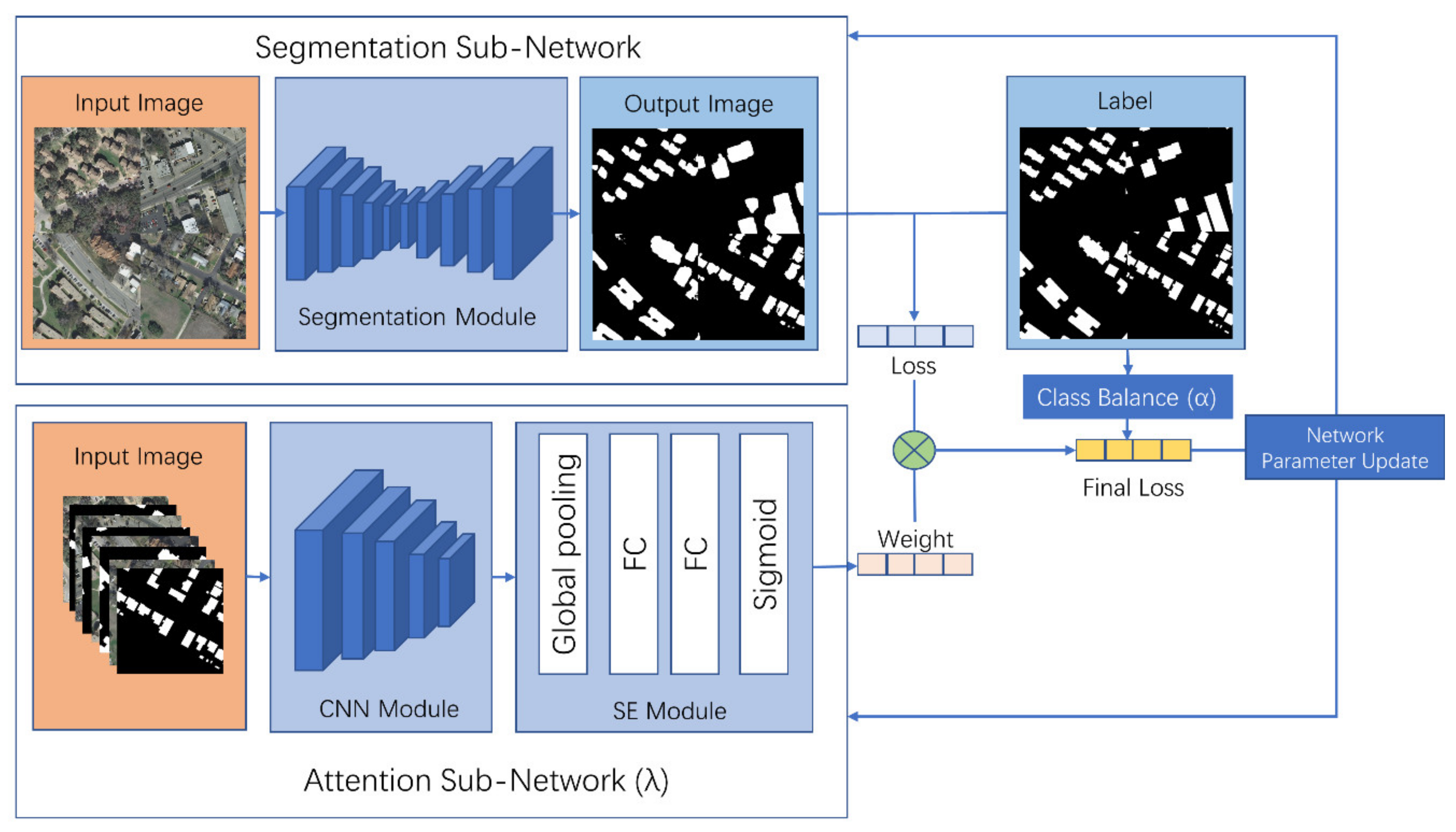
Figure 4 illustrates the overall structure of the WLN.
The overall structure of the WLN is shown in
Figure 4 with (1) the segmentation or classifier subnetwork, (2) the attention subnetwork (
Figure 5) and (3) the class-balance coefficient. The segmentation module is the deep-learning network for classification. The attention subnetwork is a convolutional neural network (CNN) structure network with an attention module that takes the image’s concatenation and its labels as an input and runs in parallel with the segmentation subnetwork. The attention subnetwork generates a weight (
) for each input sample to reweight the samples. The class-balance coefficient (
) solves the imbalance of the label class to avoid insufficient learning for classes with few samples. The final cross-entropy loss (Equation (3)), combined with the contribution of
and
, is then summed up and backpropagated to update the segmentation and attention subnetwork in combination.
In this study, we selected U-Net’s structure [
24] as the segmentation subnetwork, which other segmentation models can also replace. The attention module’s implementation form adopts the squeeze-and-excitation (SE) module [
25], which is shown in
Figure 6. The SE module was proposed to consider the relationships among channels in the feature map and provides different weights for each channel. It automatically acquires the importance of each feature channel by learning and then strengthens useful features while suppressing those not useful to the current task according to each channel’s importance. The squeeze and excitement are two critical operations in the SE module. These two operations help the SE model to capture channel-wise dependencies and significantly reduce the number of parameters and calculations [
25].
In this study, we adopt the SE module as an attention module to obtain the importance between channels and evaluate the importance of each image-training sample. The attention module takes the CNN network output as an input, and we obtain the global-feature information representing the training sample through the global-average pooling layer. Two fully connected layers are used to fuse the characteristic information of this batch of samples. Finally, the output is normalized by a sigmoid-activation function and taken as the weight for each training-sample batch. This output can provide different weights for each training-sample loss by multiplication, and the training-sample information is either strengthened or suppressed.
3.4. Class-Balance Component ()
Generally, when the network can choose which sample to learn, it first tends to choose those easy-learning samples with a low feature diversity of labels as the important samples and then choose the samples that are difficult to learn. Thus, the diversity of samples is the key to avoiding model overfitting. However, in practice, for some label errors, such as insufficient labels and missing labels, there may be many more pixels of the background class than the target class. This imbalance reduces the target class’s feature diversity and makes the whole network focus on learning the background pixels. This imbalance of classes may cause two problems: (1) the target class’s training is insufficient for those classes with few representative pixels; (2) the recall will decrease.
To overcome this problem, we created a class-balance coefficient
in the cross-entropy to balance the classes in each sample. The definition of
is shown as follows:
where
is the sum of the number of pixels of the background class in the label and
is the sum of the number of pixels of the
class in the label. As we can see, the class-balance component (
) of the background always remains 1.
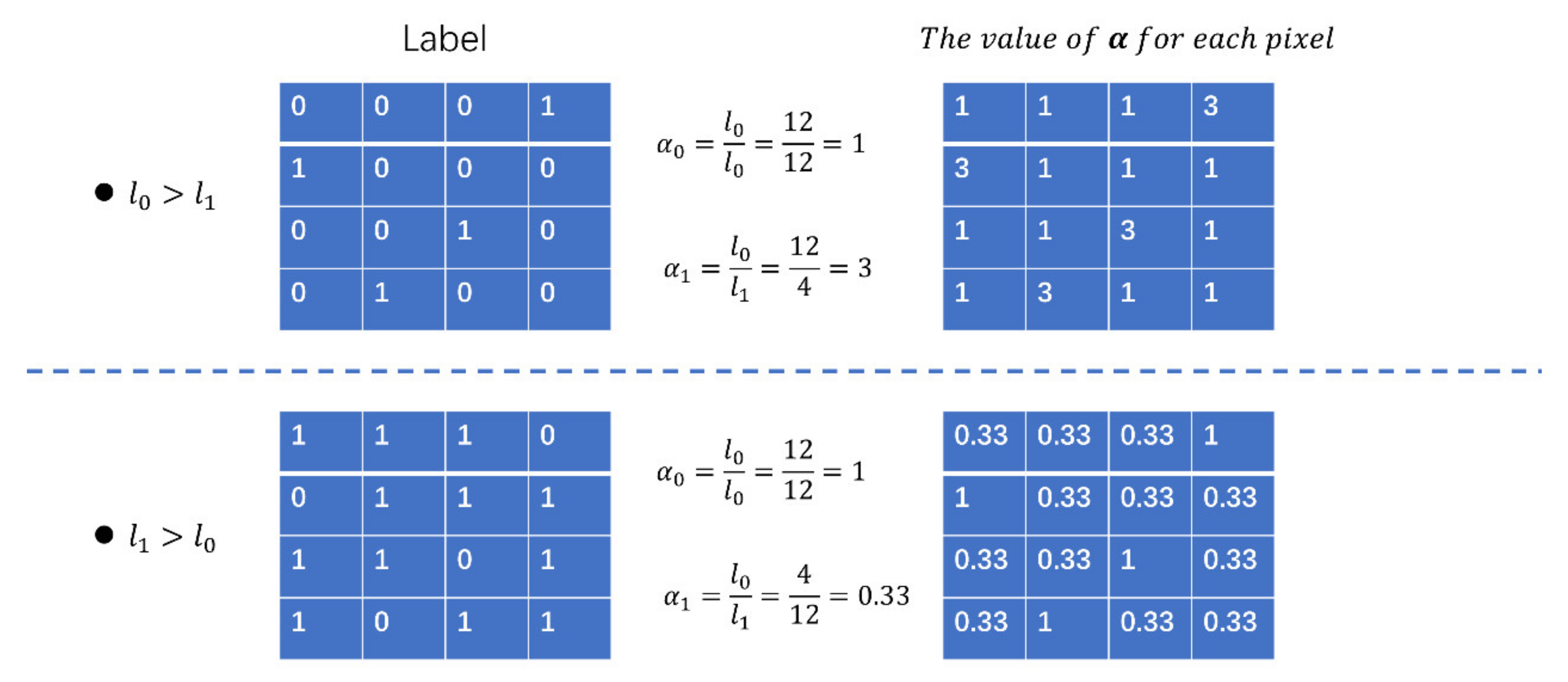
Figure 7 illustrates two simple examples of the class-balance component (
). The upper line shows the case of the insufficient label where the background (labeled as 0) is much better represented than the target class (labeled as 1). In this case, before adding the
weight, the contributions of the target class and the background class to this image’s loss value are 4/16 and 12/16, respectively. After adding the
weight, these two classes are balanced, equally contributing to the image loss value at 12/16. The same results are shown in the case of the second line of the redundant label. As we can see, the key function of the class-balance component (α) is to take one class as the reference (in most cases, it is the background class) and then adjust the other classes to make them equally important to the reference class. This will help the network to learn each class equally and avoid the prementioned problems caused by an imbalance between the different classes.
3.5. Assessment
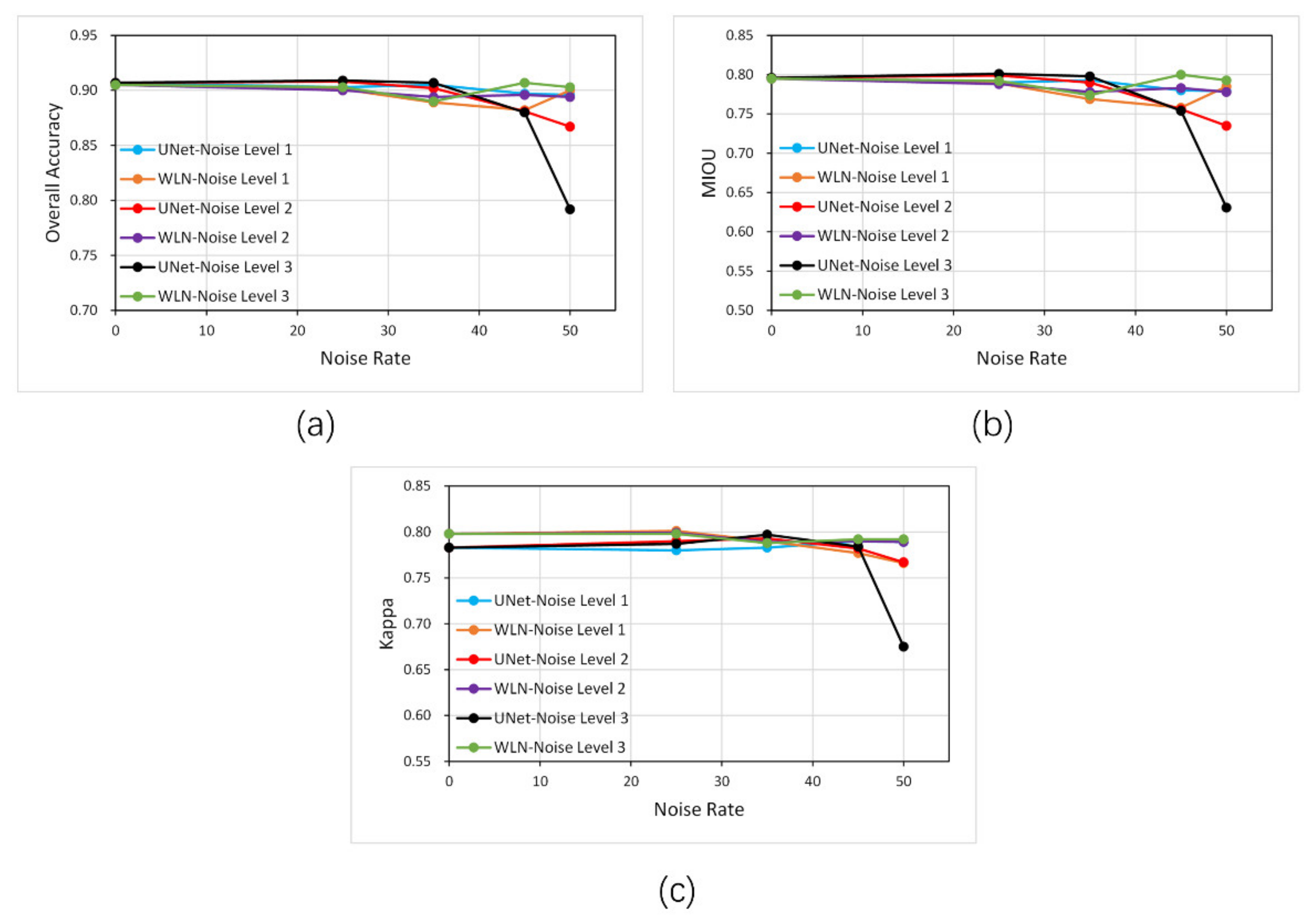
The accuracy evaluation metrics in this paper include (1) the overall accuracy, (2) the Cohen’s Kappa coefficient and (3) the Mean Intersection over Union (MIOU).
The overall accuracy is defined as the number of correctly classified pixels over the total number of pixels. It is intuitive and straightforward but may fail to assess the performance thoroughly when the number of samples for different classes varies significantly.
The Cohen’s Kappa coefficient is more robust, as it considers the probability of agreements occurring randomly. Let
be the probability of correctly classified pixels, and
be the expected probability of agreement when the classifier assigns class labels by chance; then, Cohen’s Kappa coefficient is defined as Equation (7):
Usually, we characterize as no agreement, as poor agreement, as fair agreement, as moderate agreement, as good agreement, and as almost perfect agreement.
MIOU is an important index to measure the segmentation accuracy in the field of computer-vision image segmentation. It represents the ratio of the intersection and union between the real value and the predicted value. MIOU is defined as Equation (8):
where
is the number of classifications (including background classes).
TP,
FP, and
FN correspond to the number of true positive, false positive and false negative pixels for that class, respectively. An MIOU reaches its best value at 1 and its worst at 0.
5. Discussion
Noisy labels indirectly affect the direction of the process of updating the parameters of the network by influencing the convolutional-neural-network’s loss value. Therefore, to improve the noise-immunity performance of the network, the key lies in the avoidance of the influence of noise on the network. In this study, the impact of noisy labels on the network is avoided by weighting the training samples, which is done to reduce the weight of loss values calculated from the erroneous samples. To achieve this goal, two parameters—the loss weight and the class-balance coefficient —were designed to add to the original cross-entropy loss function. In this section, we discuss the impact of and on the noise immunity of the network.
5.1. The Local Optimum Problem When We Allow the Network to Choose What to Learn
The attention subnetwork (
takes an image with a label as input and generates the loss weight
for each training sample through the CNN module and the SE module. However, we found a critical limitation if it only introduced the attention subnetwork to the framework.
Figure 12 shows the average weights of clean-label samples and noisy-label samples during the training processing with a 50% noise rate.
Figure 12a shows the average weights of the dilated noise, and
Figure 12b shows the weights for the eroded noise.
As we can see, for the dilated noise, the network cannot separate the clean samples from the noisy samples at the very beginning of training. Nevertheless, as the training batches increase, the clean samples’ loss weights increase significantly and the loss weights of the noisy samples considerably decrease. This means that the attention subnetwork () can distinguish the clean samples from the dilated noisy samples.
However, the opposite result is found when we examine the average weight for the eroded noise (
Figure 12b). The attention subnetwork incorrectly considers the noisy samples as being more essential samples, which are thus assigned with higher weights.
The reason behind this might be more universal. When we give a network the power to choose which training samples are necessary to learn, it always tends to learn samples with low feature variation. From this perspective, in the experiment of adding dilated noise, the clean samples have a lower feature variation than the noisy samples, so the network gives them higher weights. The same phenomenon was found in the case of adding eroded noise. The noise has few pixels with a lower feature variation that are easy to learn. As a result, those samples are assigned with higher weights.
This local optimum problem is similar to how the human brain works. A child also intends to learn a new object with a low feature variation at the very beginning. The training samples with more complex features will more likely be ignored. The difference between humans and the deep-learning network is that we can adjust and update our loss function (if we have) after learning the same object under different scenarios. However, for a deep-learning network, the loss function is permanently fixed for a specific task. Therefore, two possible pathways may help to overcome this problem: (1) enforcing the learning process, enlarging the training sample size, or applying modules from the enforced learning field; (2) designing a mechanism for updating the loss function.
5.2. Class-Balance Coefficient Helps to Overcome the Local Optimum Problem
Because a low-feature variation sample always shows an imbalance between the background and the foreground classes, we added the class balance coefficient to increase the loss percentage of the foreground class when calculating the loss to enforce network learning from the limited samples.
Figure 13 shows the accuracy of U-Net network (left column), U-Net with an attention subnetwork (λ) (middle column) and the WLN (right column) with different noise levels and noise rates with dilated (first row) and eroded (second row) noise during training. From the graph, we can see that when the noise rate is relatively low, all three methods can maintain high accuracy and the difference is not significant. Furthermore, when the noise rate is 50%, both the U-Net with λ and WLN methods can maintain high accuracy in the dilated-noise scenario. In contrast, the U-Net method’s accuracy curve decreases significantly. In the eroded noise, because the attention subnetwork cannot assign correct weights to clean and noisy samples, the method of only adding
will over-fit the noisy label samples, making the accuracy even lower than the original U-Net network. However, the WLN with the class balance coefficient (
) can solve this problem and maintain high accuracy. This result demonstrates that the class-balance coefficient (
) helps to overcome the local optimum problem.
In this study, the class-balance coefficient (α) designed only addresses the class-imbalance problem for each training sample. It does not address the overall imbalance problem of the entire dataset. In some circumstances, the imbalance problem may still exist between the different classes and affect the network performance. This limitation can be improved in the future.
6. Conclusions
Errors in training labels are usually hard to identify and correct, especially in remote sensing datasets across different times and locations. In this paper, we propose a general antinoise network framework, the WLN, based on the idea of weighting the loss for each training sample to minimize the impact of erroneous samples for remote-sensing image classification. The framework consists of two networks: the segmentation subnetwork and attention subnetwork. The segmentation subnetwork classifies the image pixel per pixel and calculates the output results with the labels to obtain the initial loss during the training process. The attention subnetwork generates the weight loss of a batch sample and combines it with the class-balance coefficient to prevent a class imbalance for each training sample. These three parts combine to get the final loss and backpropagate the two subnetworks to update the network parameters.
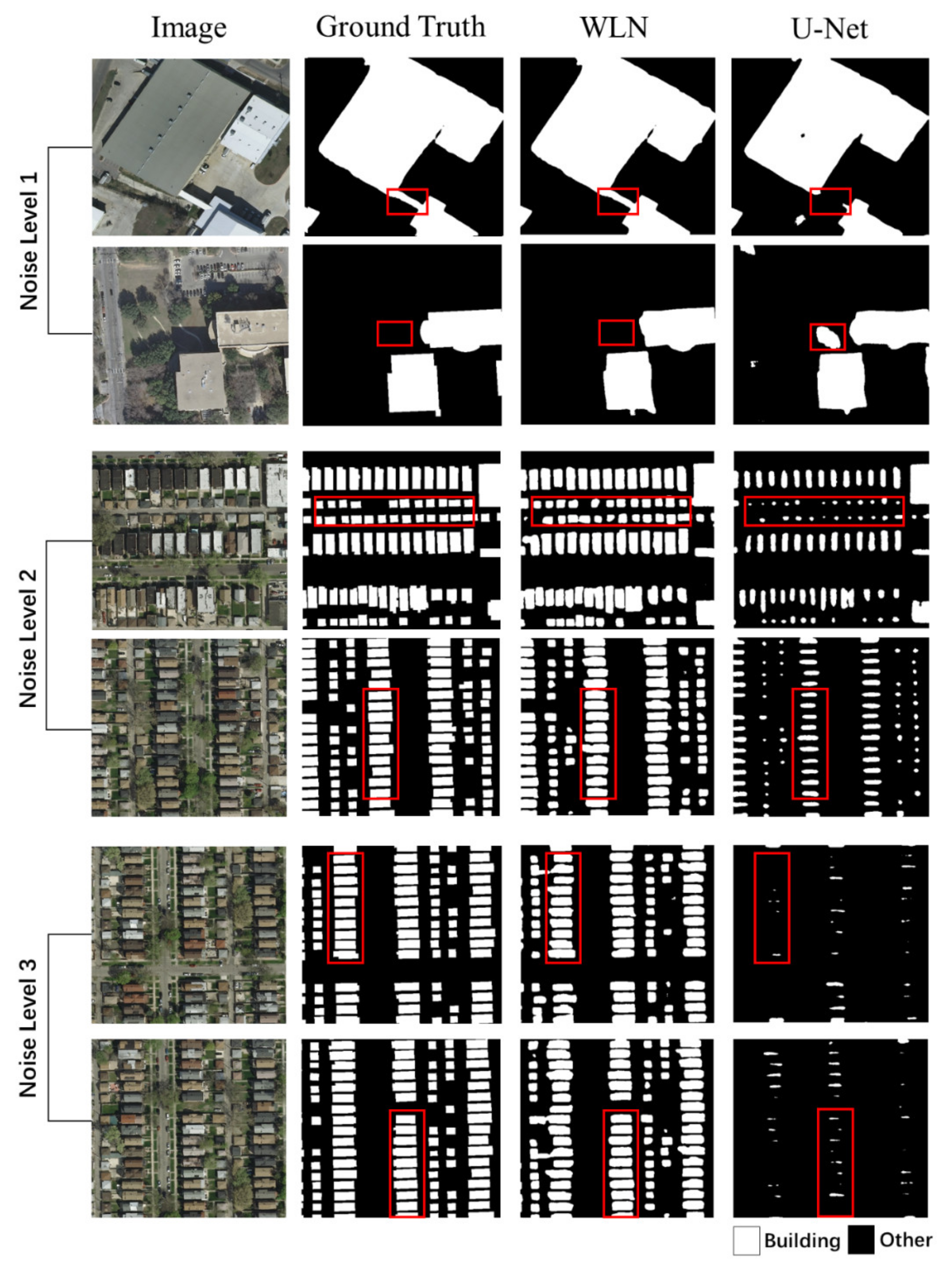
Four types of label noise (an insufficient label, redundant label, missing label and incorrect label) were simulated by dilate and erode processing to test the network’s antinoise ability. After comparing the performance of the proposed WLN to the original U-Net model when extracting buildings in the Inria Aerial Image Labeling Dataset, we found the following:
When the noise rate and noise level are low, the convolutional-neural-network is almost unaffected by the label noise, which may be due to the network’s specific noise immunity. After the training set’s label noise rate exceeds a certain threshold, the convolutional-neural-network’s accuracy decreases significantly.
For the four-label noise, our proposed method of the WLN can maintain high accuracy and outperform the original method if the sample noise rate and noise level of the data set gradually increase.
The local optimum problem was found if we allowed the network to choose which samples were essential. This phenomenon might be universal and can be relieved by adjusting the class-label imbalance by adding the class-balance coefficient.
The antinoise framework proposed in this paper can help current segmentation models avoid noisy training labels. The local optimum problem that happens when we give a network the power to choose which training samples are necessary to learn should be carefully addressed in the future. This problem might be solved by giving a deep-learning network the ability to train more intelligently and efficiently with prior knowledge in the remote-sensing field, which is also worth investigating in the future.


 ,
, 


