Article

Hyperspectral Data Simulation (Sentinel-2 to AVIRIS-NG) for Improved Wildfire Fuel Mapping, Boreal Alaska

1
Geophysical Institute, University of Alaska Fairbanks, Fairbanks, AK 99775, USA
2
Department of Natural Resources and Environment and Institute of Agriculture, Natural Recourses and Extension, University of Alaska Fairbanks, Fairbanks, AK 99775, USA
3
Department of Geography, University of California, Santa Barbara, CA 93106, USA
4
Alaska Fire Science Consortium, International Arctic Research Center, University of Alaska Fairbanks, Fairbanks, AK 99775, USA
*
Author to whom correspondence should be addressed.
Submission received: 6 March 2021 / Revised: 23 April 2021 / Accepted: 23 April 2021 / Published: 27 April 2021
(This article belongs to the Special Issue Imaging Spectroscopy of Forest Ecosystems)

Abstract

:
Alaska has witnessed a significant increase in wildfire events in recent decades that have been linked to drier and warmer summers. Forest fuel maps play a vital role in wildfire management and risk assessment. Freely available multispectral datasets are widely used for land use and land cover mapping, but they have limited utility for fuel mapping due to their coarse spectral resolution. Hyperspectral datasets have a high spectral resolution, ideal for detailed fuel mapping, but they are limited and expensive to acquire. This study simulates hyperspectral data from Sentinel-2 multispectral data using the spectral response function of the Airborne Visible/Infrared Imaging Spectrometer-Next Generation (AVIRIS-NG) sensor, and normalized ground spectra of gravel, birch, and spruce. We used the Uniform Pattern Decomposition Method (UPDM) for spectral unmixing, which is a sensor-independent method, where each pixel is expressed as the linear sum of standard reference spectra. The simulated hyperspectral data have spectral characteristics of AVIRIS-NG and the reflectance properties of Sentinel-2 data. We validated the simulated spectra by visually and statistically comparing it with real AVIRIS-NG data. We observed a high correlation between the spectra of tree classes collected from AVIRIS-NG and simulated hyperspectral data. Upon performing species level classification, we achieved a classification accuracy of 89% for the simulated hyperspectral data, which is better than the accuracy of Sentinel-2 data (77.8%). We generated a fuel map from the simulated hyperspectral image using the Random Forest classifier. Our study demonstrated that low-cost and high-quality hyperspectral data can be generated from Sentinel-2 data using UPDM for improved land cover and vegetation mapping in the boreal forest.

Graphical Abstract

1. Introduction

Wildfires are of great importance when it comes to plant succession, natural regeneration, reducing debris accumulation, maintaining ecosystem health, diversity, nutrient cycle, and energy flow [1]. Since excess of anything causes harm, increase in wildfire frequency and area burned also poses a risk to the ecosystem’s health and diversity. Severe wildfires are occurring globally every year, causing unprecedented ecological and economic damage. In 2019, a massive fire occurred in the Amazon rainforest, which attracted global attention. Again, in 2020, the Amazon forest suffered a severe loss from wildfires that burned an area of approximately 20,234 sq. km [2]. In the same year, Australia recorded a huge bushfire that burned an area of around 186,155 sq. km and nearly 3 billion animals were displaced [3]. In 2020, 17,230 sq. km in California burned from wildfires that spread over the West Coast of the United States, making 2020 the largest wildfire season recorded in California’s modern history [4].
Alaska, the northernmost state of the US, has 509,904 sq. km of forested land [5]. Wildfires are a natural and essential part of Alaskan ecosystems. Nonetheless, wildfires in Alaska are increasing in frequency, area burned, and severity, mirroring the global increase in wildfire events [6,7]. In the last two decades (2001–2020: 127,671 sq. km), wildfires in Alaska have burned 2.5 times more forest than the previous two decades (1981–2000: 57,060 sq. km) [7]. In 2019, Alaska had 719 wildfires that burned nearly 10,500 sq. km of forest [8], making it the 10th largest fire year in recorded history. Many of these fires were near major population centers along the Wildland Urban Interface (WUI). The societal impacts of WUI fires (i.e., risk to life and property, unhealthy air quality, and cost of suppression) can be reduced if fire managers have access to reliable fuel maps (that is, boreal vegetation maps) for the development of effective fuel and fire management strategies [9,10]. Enhanced fuel mapping is also essential for the strategic planning of wildfire mitigation [4].
Remote sensing is a viable approach to map the vegetation of the boreal forests, considering the region’s remoteness and vastness [11,12,13,14,15]. The Landscape Fire and Resource Management Planning Tools Project (LANDFIRE) provides geospatial products to state and federal fire suppression agencies for wildfire mitigation [16,17]. The traditional map products provided by the LANDFIRE for Alaska’s boreal domain lack granularity needed for fire management at the fire incident (meter) scale. LANDFIRE products are derived from Landsat 8 multispectral data, which has few spectral bands and moderate spatial resolution (30 m). Additionally, these products have classification accuracies in the range of 20% to 45%, leaving considerable room for improvement [18]. In Alaska, effective management of fuels and active fire requires improved fuel maps at the species level.
Advancements in airborne hyperspectral remote sensing provide an efficient approach to retrieve essential information for better characterization of forest fuels [14,19,20,21]. A number of studies have shown that hyperspectral data is much more effective than multispectral data for detailed vegetation mapping at species or stand scales [14,22,23,24,25,26,27,28,29,30]. The narrower bandwidths and improved spatial resolution of airborne hyperspectral datasets makes them much more effective than multispectral datasets at distinguishing visually similar vegetation classes. However, one of the major challenges with airborne hyperspectral technology is the cost of data acquisition. Currently, available hyperspectral datasets collected as part of the NASA Arctic-Boreal Vulnerability Experiment (ABoVE) and Goddard’s LiDAR, Hyperspectral, and Thermal Imager (G-LiHT) programs cover only a small portion of the boreal domain. There is a need for greater spatial coverage and frequency while providing detailed spectral information similar to hyperspectral datasets.
Few studies have attempted to address this need through the simulation of hyperspectral data using publicly available multispectral datasets [31,32,33]. Zhang et al. [33] proposed a spectral response approach that used the Universal Pattern Decomposition Method (UPDM) for hyperspectral simulation from Landsat 7 Enhanced Thematic Mapper Plus (ETM+) and Moderate Resolution Imaging Spectroradiometer (MODIS) data. Liu et al. [31] followed a similar approach in which they simulated 106 hyperspectral bands from EO-1 Advance Land Imager (ALI) multispectral bands using standard ground spectra of water, vegetation, and soil. They performed Land-Use and Land-Cover (LULC) classification using the Spectral Angle Mapper (SAM) classifier and obtained an overall accuracy of 87.6% from the simulated hyperspectral data compared to 86.8% from ALI data. Tiwari et al. [32] used a similar simulation technique to generate a LULC map for a site located in northern India. They simulated hyperspectral data from Landsat 8 Operational Land Imager (OLI) multispectral data using spectra of vegetation, water, and sand as the endmembers. Using a SAM classifier, they obtained an overall accuracy of 69.4% from simulated hyperspectral data compared to 63.0% accuracy from OLI data.
Airborne Visible/Infrared Imaging Spectrometer-Next Generation (AVIRIS-NG) is the most advanced imaging spectrometer developed by NASA’s Jet Propulsion Laboratory (JPL). The AVIRIS-NG sensor offers a higher signal-to-noise ratio, excellent system calibration, and more accurate image geo-rectification [34]. The data are available at wavelengths ranging from 380 to 2510 nm with a 5 nm bandwidth, at spatial resolutions of a few meters (depending on flying height) (Figure 1). Previous studies [31,32] attempted to simulate Hyperion data from EO-1 ALI and Landsat 8 OLI multispectral datasets in order to improve LULC classification. The Hyperion sensor flew on the EO-1 satellite from 2000 to 2017, and it has 242 spectral bands in the range of 400–2500 nm and 30 m spatial resolution [35]. Simulation of AVIRIS-NG data is as yet unexplored, and that offers an opportunity to explore AVIRIS-NG data simulation to generate low-cost hyperspectral data for improved vegetation and LULC mapping. Sentinel-2 is the most recent multispectral sensor with global coverage and open data access. It has 13 spectral bands (spatial resolution: 10 m for visible-near infrared bands, and 20 m for SWIR bands) (Figure 1), especially the presence of red edge, NIR, and SWIR bands, and higher spatial resolution makes it apt for hyperspectral simulation [36,37,38].
The overarching goal of this study is to generate low-cost and high-quality hyperspectral data from widely available Sentinel-2 data to meet the need for greater spatial and temporal coverage of hyperspectral data for improved vegetation and fuel mapping in the boreal forest. In this study, we simulated an AVIRIS-NG hyperspectral dataset from a Sentinel-2 multispectral dataset using the UPDM spectral reconstruction approach for the boreal forest of Alaska. Since birch (Betula papyrifera: a deciduous species) and spruce (Picea mariana: a coniferous species) are the dominant trees at the test site, and accurately distinguishing coniferous and deciduous forest is essential for fire behavior modeling, we used the spectra of birch, spruce, and gravel (bare ground and rocky areas) as the endmembers for simulation. We visually and statistically compared the results of the simulated hyperspectral dataset with the AVIRIS-NG dataset.

2. Materials and Methods
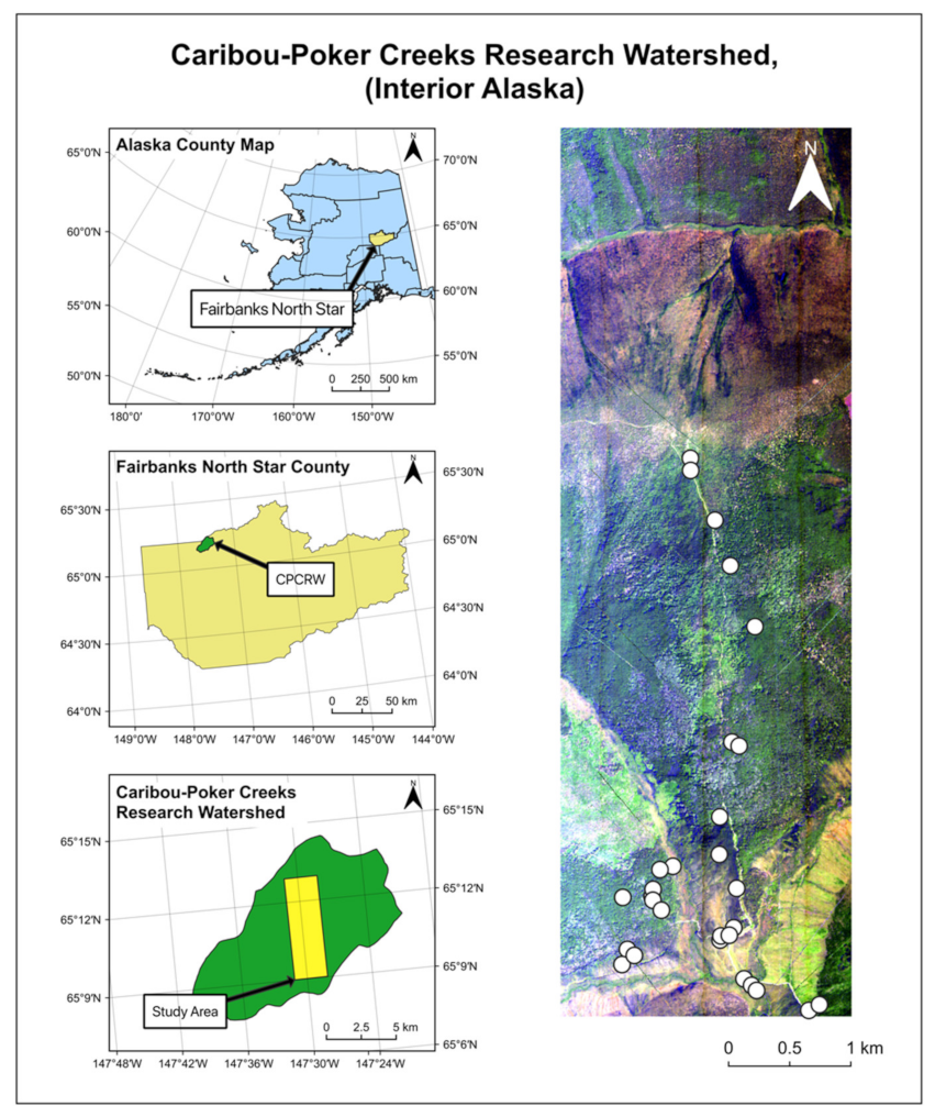
2.1. Study Area

The Caribou-Poker Creeks Research Watershed (CPCRW) is spread over a 104 square km area reserved for scientific study, including ecology, meteorology, and hydrological research. CPCRW is located in interior Alaska, 64 km northeast of Fairbanks (65.15° N, 147.50° W). We selected a test site within CPCRW for this study (Figure 2), where we had availability of an AVIRIS-NG scene. The air temperature varies from winter minima of –50 °C to summer peaks reaching 33 °C, with a long-term annual mean temperature of −3 °C. This area is typically under snow cover between October and April. The mean annual precipitation is about 262 mm, and 30% of it is in the form of snowfall [39].

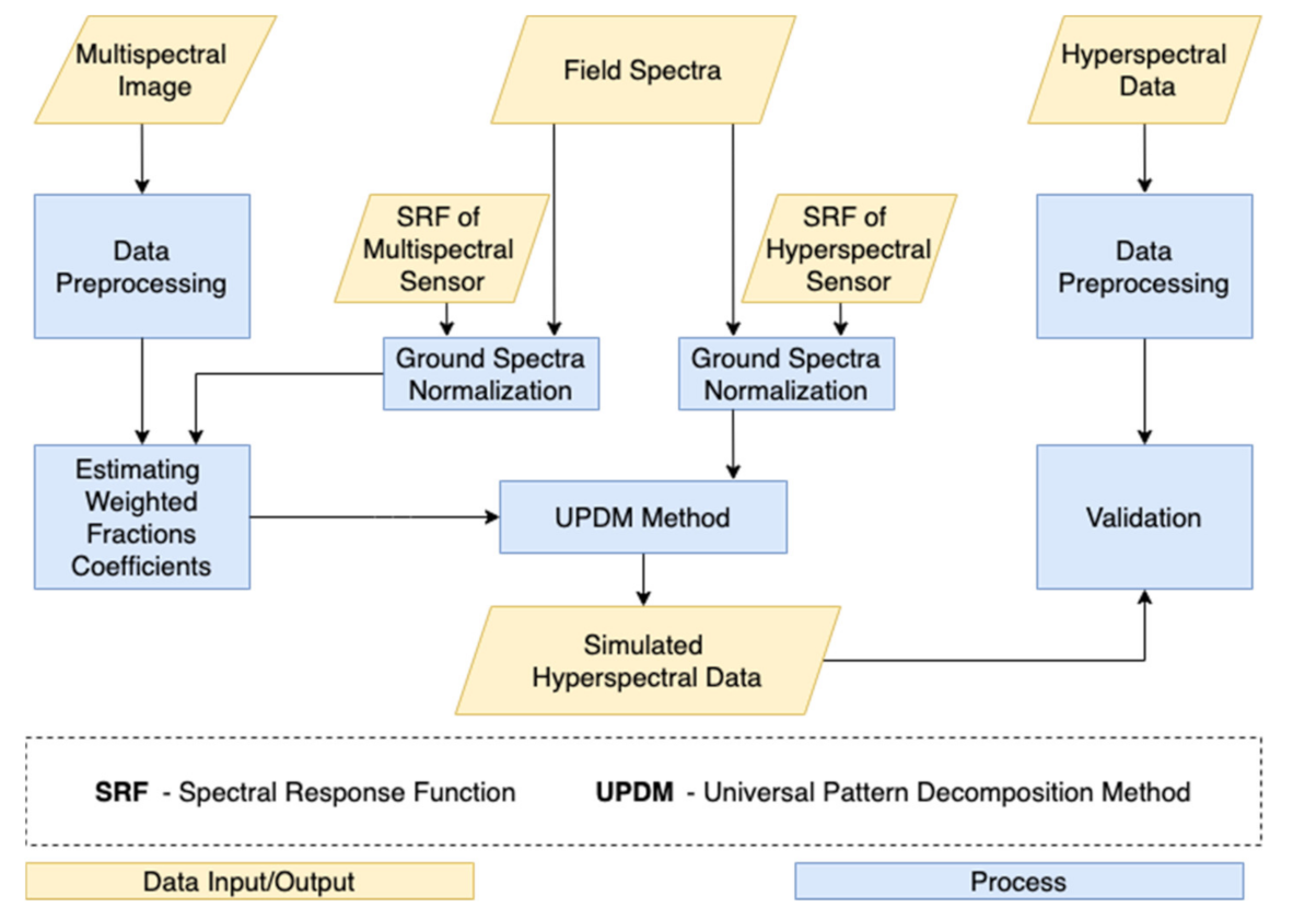
2.2. Processing Workflow

Figure 3 shows the processing workflow. The input data consists of Sentinel-2 multispectral imagery, the Spectral Response Function (SRF) of Sentinel-2 and AVIRIS-NG sensors, and spectra of birch, spruce, and gravel collected using the Spectral Evolution® PSR + 3500 hand-held spectroradiometer (Spectral Evolution Inc., Lawrence, MA, USA). The PSR + 3500 provides reflectance data in the range of 350–2500 nm at 1 nm spectral resolution for a total of 2151 channels.
The methodology is divided into four major phases: (1) field data collection, (2) remote sensing data preprocessing, (3) hyperspectral simulation, and (4) validation.

2.3. Field Data Collection

We collected all field data during the summer of 2019 and 2020. We collected several leaf spectra samples for different tree/shrub species using a PSR + 3500 Field Spectroradiometer. We collected the field spectra on 17 August 2019 between 11:00 to 14:00 (weather: sunny with clear sky; solar noon: 14:06). We collected spectra holding the optic 2 inches away from leaves and collected a minimum of 4 samples for each endmember. We used the mean endmember spectra in the simulation [20].
For the image classification, we recorded tree locations from stands where one type of tree species was present in clusters or groups. This enabled us to identify near to pure pixels for training and testing the image classifier as well as to reduce the background noise. In Figure 2, the white dots denote the locations of the sample sites. We surveyed sample sites using a Trimble Real-Time Kinematic (RTK) Global Positioning System (GPS) unit that offers millimeters positional accuracy. The study site (CPCRW) is part of protected state forests. The vegetation change at this site due to natural succession takes places at multiple decade to century time scales. However, dramatic vegetation change can occur due to wildfires or insect outbreaks. During the field survey, we did not observe any evidence of fire or insect outbreak within the study area. Also, we are not aware of any report of forest damage or change in the study areas since 2018 (when the AVIRIS-NG image was collected). So, we are certain that the use of field data collected in 2019 and 2020 for image classifier training and classification accuracy assessment are reasonable and resulted in accurate and reliable map products.

2.4. Remote Sensing Data Preprocessing

2.4.1. Multispectral Data Preprocessing

We used atmospherically corrected Sentinel-2 Level-2A reflectance data available from the European Space Agency (ESA) Copernicus Open Access Hub [38] acquired on 24 July 2018. Sentinel-2 bands are available in different resolutions. The visible bands (band 2, 3, and 4) and the NIR band (band 8) have 10 m resolution, while the vegetation red edge bands (bands 5, 6, 7, and 8A) and the SWIR bands (band 11 and 12) have 20 m resolution. We resampled the pixels of all the bands with 20 m resolution to the lowest pixel resolution of 10 m to keep the pixel counts the same for all bands in the simulation. We removed coastal aerosol, water vapor, and cirrus bands from the data, and layer-stacked the remaining bands. From the stacked data, we clipped out the study area. Sentinel-2 data preprocessing was performed in the Quantum GIS (QGIS) software version 3.4 developed by the QGIS development team [40].

2.4.2. Hyperspectral Data Preprocessing

In this study, we used an AVIRIS-NG level 2 [41,42] product acquired on 21 July 2018, which covers a portion of CPCRW. The AVIRIS-NG scene has 425 bands and 5 m spatial resolution. Some of these bands were removed since they were from wavelengths dominated by water vapor and methane absorption and contained noise due to atmospheric scattering and poor radiometric correction. We refer to such bands as bad bands. All the bad bands were removed from the original scene using the ENVI classic software [43]. We manually visualized each band and removed the noisy bands, resulting in a 332-band subset. Table 1 identifies all the bands which we removed from the original AVIRIS-NG data [44]. We used a spatial subset of the AVIRIS-NG scene for the study.

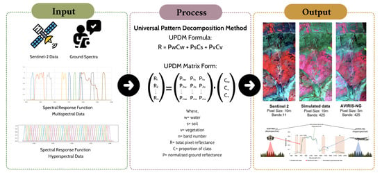
2.5. Hyperspectral Simulation

The process of hyperspectral data simulation is divided into three steps: (1) ground spectra normalization, (2) calculation of weighted fractional coefficients, and (3) hyperspectral data simulation.

2.5.1. Ground Spectra Normalization

We used ground spectra from multiple locations for all three endmembers: birch, spruce, and gravel, and used their mean spectra in the simulation. We normalized each endmember spectrum by convolving it with the spectral response function (SRF) of both the multispectral and the hyperspectral sensors. The SRF is the probability that the sensor will detect a photon of a given frequency and it depends on the central wavelength and the bandwidth of the sensor [45]. The Sentinel-2 SRF was obtained from the Sentinel-2 document library [46]. The SRF of AVIRIS-NG was not directly available, but the Full Width at Half Maximum (FWHM) values were available. We used a Gaussian function to generate the AVIRIS-NG SRF [31], assuming that the peak of the Gaussian curve with respect to the central wavelength is at 1 (Equation (1)). We used Equation (2) to determine the bandwidth, σ .
g λ ¯ i , σ i = e x p λ ¯ i λ 2 2 σ 2
σ i = F W H M i 2 2 l n 2
where:
g   = gaussian function
i = band number
λ ¯ = central wavelength
σ = bandwidth
λ = wavelength
F W H M i = Full Width at Half Maximum values for each band
Using the above Gaussian function, we constructed the SRF for all the bands of AVIRIS-NG.

2.5.2. Calculation of Weighted Fractional Coefficients

In this step, we used the Universal Pattern Decomposition Method (UPDM), a linear unmixing method, used to model landcover in proportion to the endmember spectrum present in each pixel of the image [31,32,47]. This method uses normalized ground spectra and the reflectance from multispectral data to estimate weighted fractional coefficients. This method assumes that each pixel of the multispectral data is a linear mixture of normalized ground spectra in the image using Equation (3):
R i = Σ j = 1 n ( P i j .   C j )
where:
i = Number of bands (1 to m )
j = Number of endmember or class (1 to n )
R i = Reflectance value of i t h   pixel in the image
P i j = Field spectra of the jth component, i.e., classes
C j = Fraction of coefficient of the j t h   component within the pixel
We can represent the linear unmixing equation for all the pixels in the image in matrix form using Equation (6):
R = P C
R = P b C b + P s C s + P g C g
R 1 R 2 R n   = P 1 b P 1 s P 1 g P 2 b P 2 s P 2 g P n b P n s P n g . C b C s C g
where:
R = total pixel reflectance
C = proportion of class
P = normalized ground reflectance
b = birch
s = spruce
g = gravel
n = number of bands
For a multispectral sensor, we can represent Equation (4) as:
R M = P M C M
C M can be calculated via inversion by applying the least squares method in Equation (7):
C M = ( P M   T .   P M ) 1 .   P M   T .   R M
We calculated C M   using the multispectral data and Equation (8). It is the fraction of each endmember in a pixel (i.e., fractional coefficient) in the form of a matrix for the whole image. R M is the matrix with reflectance values from Sentinel-2 multispectral data and P M is a matrix that contains the normalized ground spectra (birch, spruce, and gravel).

2.5.3. Hyperspectral Data Simulation

This step requires the fractional coefficient image of the multispectral data and the SRF of the hyperspectral sensor as inputs. For a pixel, the proportion occupied by an endmember will be the constant at a constant spatial resolution, irrespective of the sensor type. The simulated hyperspectral data will have the same spatial resolution as Sentinel-2 data. Therefore, the fractional coefficients ( C M ) calculated using the multispectral data (Section 2.5.2.) will be the same. We also normalized the ground spectra of the three classes using SRF of hyperspectral data, as mentioned in Section 2.5.1. By using these two matrices, we calculated the simulated reflectance values using Equation (9):
R H = P H .   C H
Since C H = C M , we can replace C H in Equation (9) with value C M from Equation (8):
R H = P H .   ( P M   T .   P M ) 1 .   P M   T .   R M
Here, in Equation (10), R H contains the reconstructed band values of the hyperspectral data, in the form of a matrix. This matrix was written as a raster file (GeoTiff format).
We performed hyperspectral data simulation in Python 3 [48] using Pandas library [49] to handle the data in a data frame format. Further, we used the Numpy library [50] to perform the matrix calculations. Finally, we used the GDAL library [51] to work with raster, especially to read and write the image data.

2.6. Validation

We validated the simulated hyperspectral data using visual interpretation, statistical analysis, and by comparing image classification results.

2.6.1. Visual and Statistical Analysis

We observed spectral signatures of different classes collected from AVIRIS-NG data, Sentinel-2 data, and simulated hyperspectral data, and further validated them using the field data. We compared the reflectance values and visually analyzed the pattern of the spectra. We also calculated the Pearson’s correlation coefficient to evaluate the relationship between the spectra of simulated hyperspectral data and AVIRIS-NG data.
We performed a visual comparison using the Colored Infrared (CIR) image, also known as False-Color Composite (FCC) image, generated with bands 97, 56, and 36 as RGB for the AVIRIS-NG and simulated hyperspectral image, and with bands 8, 4, and 3 as RGB for the Sentinel-2 image. We considered and analyzed different areas of interest based on how they differ visually in terms of the landcover pattern.
We computed the band-to-band correlation between the simulated hyperspectral data and the AVIRIS-NG data. This analysis indicated the degree of similarity to AVIRIS-NG bands and allows us to identify bands with low correlation values.

2.6.2. Classification

We classified the simulated hyperspectral data, AVIRIS-NG hyperspectral data, and Sentinel-2 data, and then compared results to validate the simulated hyperspectral data. Due to the presence of a large number of bands in both hyperspectral datasets, it was essential to select a suitable classifier. We chose a Random Forest (RF) classifier [52] to perform the classification due to its ability to deal with many features (bands). Another advantage of using RF was that there are only two user-defined parameters: the number of decision trees and the number of features per subset. RF produces each decision tree independently, and it splits each node of the decision tree using a number of features [53]. We performed RF classification using the ‘RandomForestClassifier’ function of the scikit-learn library [54] in Python 3, and both user-defined parameters were kept constant in all three cases. A low number of decision trees tend to create a bias in the result when dealing with multidimensional datasets, while with a high number of trees, the error gets stabilized. Hence, we took 500 decision trees for training the classifier [53]. We obtained the features per subset by calculating the square root of the total number of bands. Therefore, in our case, the number of features per subset will be √(332) ≈ 18. We trained the RF classifier using the field survey locations as a guide and performed species-level classification in all three cases.
We surveyed vegetation at 29 plots in the field, of which 30% were used for testing the classification accuracy while the remaining plots were used to train the classifier. The total number of pixels surveyed on the ground for each class are presented in Table 2.
When using a machine learning classifier for LULC classification, it is preferable to have the same number of pixels in all the classes [55]. In our case, the number of pixels in the training and testing datasets for each class was different (Table 2), so to balance the pixels in all the classes, we applied the Synthetic Minority Oversampling Technique (SMOTE) [56]. SMOTE is an oversampling technique that duplicates the classes having fewer samples using the minority data population. While it increases the data, it does not add any new information to the machine learning model.
For accuracy assessment of the three classification outputs, we calculated confusion matrices [57], which indicate how many pixels are correctly identified. From the confusion matrix, we can evaluate the accuracy of each class in terms of producer accuracy, user accuracy, and kappa value. Producer accuracy identifies how often the real features on the ground are correctly shown on the map. Conversely, the user accuracy indicates how often the class on the map will be present on the ground.

2.7. Fuel Type Classification

We classified the simulated hyperspectral data using a Random Forest classifier to generate a fuel map of the study area. We identified different fuel classes from the ground data based on the fuel guide provided by the Alaska Wildland Fire Coordinating Group [58]. We used ground data from 58 surveyed field plots in 2019 and 2020 and were able to identify a total of 7 fuel classes.

3. Results

We simulated 332 bands of AVIRIS-NG based on the Sentinel-2 multispectral data and performed species-level as well as fuel-level classification. Figure 4 shows color infrared (CIR) images of the simulated hyperspectral data along with the AVIRIS-NG and Sentinel-2 data at the study site. Visual comparison of AVIRIS-NG and simulated hyperspectral data demonstrated high spatial and spectral similarity (Figure 4). Since these images are in CIR composition, broadleaf vegetation appears bright red. The central region of the study site mostly consists of deciduous forest and dense canopy. The top and the bottom region of the study site are dark green due to the dominance of needle-leaved species (mostly black spruce).

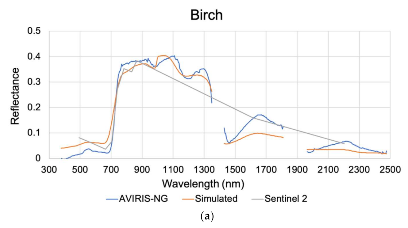
3.1. Spectral Profile Comparison

The simulated hyperspectral data capture most of the absorption features and reflectance patterns present in the original AVIRIS-NG data. Figure 5 shows the comparison between spectral profiles of birch vs. spruce. The spectral signatures were selected from the regions where clusters of respective species were available on the ground.
We found correlation coefficients (r) of 0.97 and 0.92 between the reflectance values of the simulated hyperspectral data and the AVIRIS-NG data for birch and spruce, respectively. We also observed that for both cases, the spectra almost overlapped in the NIR region, while there were some minor deviations in the visible and the SWIR regions. The strong positive correlations confirm that the simulated hyperspectral data is capturing most of the absorption features and reflectance patterns present in the original AVIRIS-NG data.

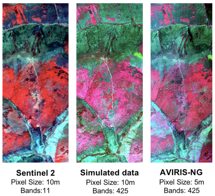
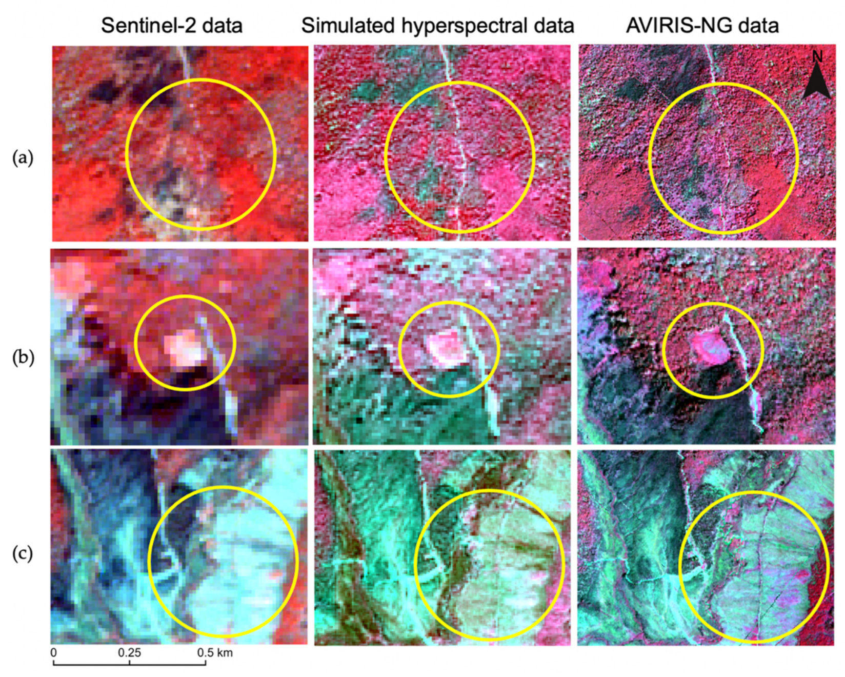
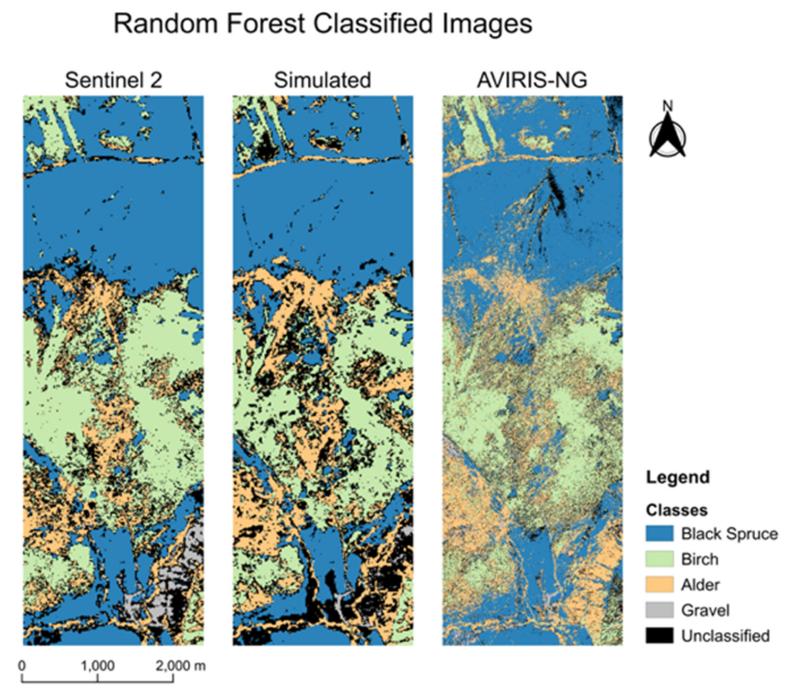
3.2. Visual Interpretation

The simulated hyperspectral data match very well with the actual hyperspectral data upon visual inspection (Figure 6). In Figure 6a, a trail can be identified in the middle of the study area. In the Sentinel-2 image, the trail was hardly visible, and it was difficult to discriminate between the different vegetation classes, while in the case of the simulated hyperspectral image, the vegetation classes were easily differentiable, and the trail is clearly visible (enlarged in yellow circle). Indeed, the simulated hyperspectral image conveys a level of detail that looks similar to that of the original AVIRIS-NG image. In Figure 6b, we highlight a square patch of young alder and birch on the ground (in the yellow circle). In the simulated hyperspectral data and AVIRIS NG image, the features of the patch are easily distinguishable, but less so in the Sentinel-2 image. A third area with patches of low-growing vegetation including moss, cottongrass, tussock, and low shrub (blueberry and dwarf birch) was distinguished by the simulated hyperspectral image and AVIRIS-NG but not in the Sentinel-2 image (see yellow circle, Figure 6c). In the simulated hyperspectral image, more features and vegetation classes can be identified, similar to the AVIRIS-NG data. In contrast, in Sentinel-2, most of the area is covered by a single class.

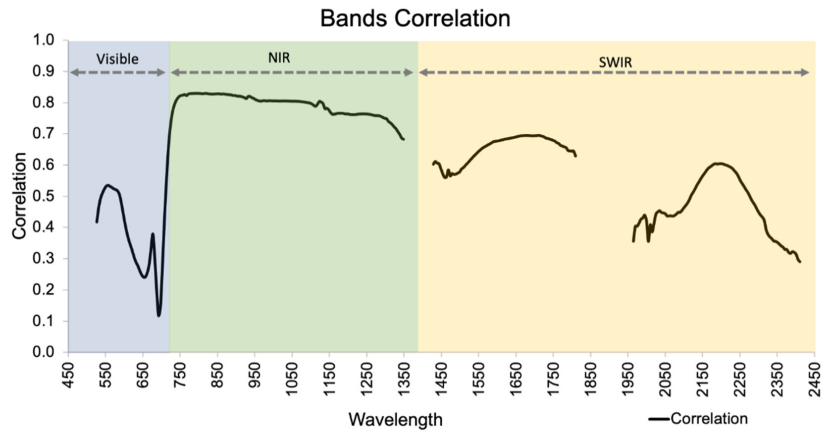
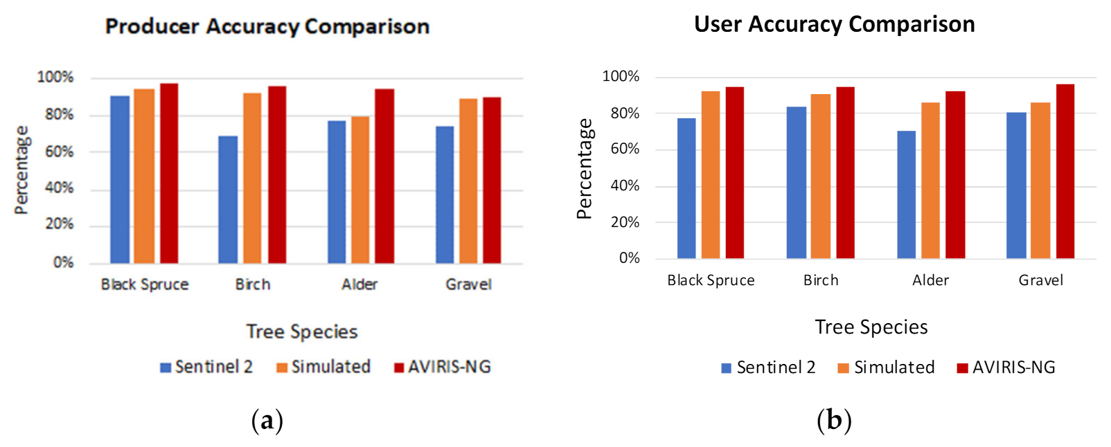
3.3. Statistical Analysis

In the simulated hyperspectral image, most bands showed good correlation with AVIRIS-NG, while a few showed a low correlation (Figure 7). There was high correlation in the NIR region, while correlation was poor in the visible and SWIR ranges.

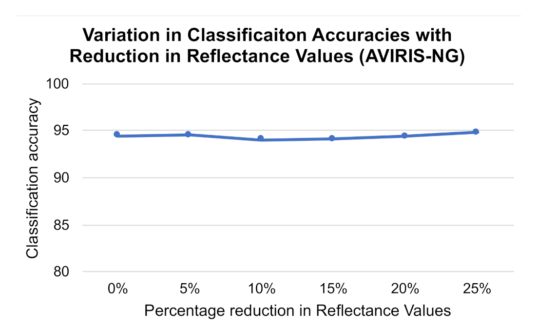
3.4. Image Classification
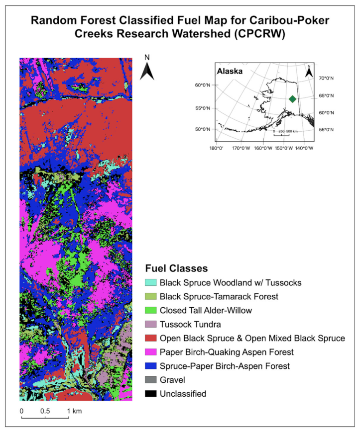
Figure 8 highlights the results of species-level Random Forest classification. We performed the classification with four major classes: black spruce, birch, alder, and gravel. We obtained higher classification accuracy for simulated hyperspectral data than Sentinel-2 data. Table 3 shows the accuracy assessment of the three classification outputs. Since we considered only near to pure pixels for both training and testing, all three classes showed good classification accuracies. AVIRIS-NG performed the best with 94.6% accuracy and kappa = 0.93, followed by the simulated hyperspectral data showing 89% accuracy and a kappa value of 0.85, and finally Sentinel-2, with 77.8% accuracy and a 0.70 kappa value (Table 4).
For all the classes, the classified AVIRIS-NG dataset gave the best results for the user and the producer accuracy (Figure 9). Also, there was a substantial improvement in the accuracy of all the classes in the case of simulated hyperspectral data results when compared to the Sentinel-2 results.
To assess the effects of the different reflectance values on image classification accuracy, we reduced the reflectance of the original AVIRIS-NG data by 5% to 25% at an interval of 5% at each step and performed image classifications and accuracy assessments. We did not find any significant change in classification accuracy (Figure 10) due to a reduction in reflectance values. Based on these observations, we conclude that (up to 25%) differences in reflectance values (between original AVIRIS-NG and simulated hyperspectral data) have little or no impact on overall image classification accuracy.

3.5. Fuel Map

Upon fuel type classification, we found that the simulated hyperspectral data provided 65% overall accuracy, while classification accuracy of Sentinel-2 data was 56%. Figure 11 shows the fuel map, where we classified a total of 7 fuel types.

4. Discussion

This study demonstrated the potential of simulated hyperspectral data for the purpose of forest fuel mapping. Visual inspection of RGB composites shows that the simulated hyperspectral image is similar to AVIRIS-NG image in texture, tone, and shading. The spectral comparison shows that the band-to-band correlations vary by wavelength, with highest correlations found in the NIR region, moderate in the SWIR region, low in the visible region, and very low along the red-edge region (Figure 7). This is likely due to NIR scattering and non-linear mixing. In a study by Roberts et al. [19], non-linear mixing results in residual errors along the red-edge. These errors are present because plants do not scatter much in the visible region but do scatter in the NIR region. Since the NIR dominates the mixture, this results in high NIR correlation, but lower visible and SWIR correlation. We can minimize this problem by using field spectra collected at a scale that includes multiple scattering [20].
We found that the difference in reflectance values over the near infrared region (700–1400 nm) is relatively small, and the visual pattern of the spectra is also similar. Notable differences in the reflectance values in the SWIR region (1500–1800 nm) were observed. Zhang et al. [47] performed a similar simulation in which the simulated spectra showed little to no difference below 1000 nm, but a notable difference was found above 1000 nm wavelength when compared with the original spectra. This difference could be due to the variation in spatial resolution, especially in the SWIR region, 20 m for Sentinel-2 vs 5 m for AVIRIS-NG. The pixel resampling also contributed to the difference in reflectance value, where we resampled the 20 m pixel size of the Sentinel-2 SWIR region to a 5 m pixel size. The atmospheric corrections applied to Sentinel-2 data and AVIRIS-NG data were different due to the fact that Sentinel-2 data was captured from space while AVIRIS-NG data was captured from an aircraft at an altitude of 10.6 km, and that the data had different acquisition dates [59]. Therefore, the instantaneous field of view and the atmospheric corrections for these sensors are appreciably different, contributing to differences in reflectance values [31,60].
Visually, the simulated hyperspectral data appears similar to the AVIRIS-NG data, with minute spatial details preserved. The overall observation is that the simulated hyperspectral imagery provides an improved spectral resolution from Sentinel-2 imagery. We used three endmembers, and yet, areas of different vegetation cover types (moss, blueberry, and dwarf birch), which are not distinguishable in Sentinel-2 data, are clearly differentiable in the simulated hyperspectral data. In an open forest setting, woody materials such as downed logs, standing tree boles, dry grass, and leaf litter, together referred to as non-photosynthetic vegetation (NPV), can contribute to the reflectance of an image pixel [19]. In this study, we did not use NPV as an endmember. It would be interesting to further experiment with this simulation by adding a NPV variable in the UPDM equation as an endmember. Shade is another endmember that could be added to the equation, especially when working on the boreal forest where the canopy density is low.
In agreement with Liu et al. [31] and Tiwari et al. [16], we obtained higher classification accuracy from simulated hyperspectral data than the Sentinel-2 data (Table 4). The majority of misclassifications were gravel pixels. Gravel is mostly present on the narrow trails, and the young alder and birch patches present along the gravel trails were responsible for the misclassifications. Gravel was also misclassified with black spruce due to the open canopy structure, resulting in training pixels which included portions of ground reflectance reducing signal purity. In the case of Sentinel-2 results, birch was often misclassified with alder because of their spectral similarity, while simulated hyperspectral data performed better in discriminating these two species. This finding supports the notion that the simulated hyperspectral data can capture the minute spatial and spectral details of real hyperspectral data. The strength of this simulated dataset lies in providing spectrally enhanced data which can be used for detailed LULC classification. Tiwari et al. [32] used the UPDM technique to simulate Hyperion data for land cover classification at a test site in northern India, and obtained 6.45% improvement in mapping accuracy over ALI multispectral data. Likewise, in this study, we successfully simulated AVIRIS-NG hyperspectral data for species-level and fuel-level vegetation mapping at a test site in the boreal forest and obtained 11.2% improvement in mapping accuracy over Sentinel-2 data.
When we performed the fuel type classification, the simulated hyperspectral data achieved an overall classification accuracy of 65%. Smith et al. [14] carried out a detailed fuel type mapping from the original AVIRIS-NG data for the same study site and reported an accuracy of 61%. This suggests that simulated hyperspectral data can provide comparable mapping accuracy to real AVIRIS-NG data. Overall, these findings suggest that the generation of fuel maps from low-cost simulated hyperspectral data using the UPDM is feasible for Alaskan boreal forests.

5. Conclusions

The study aimed to simulate hyperspectral data from multispectral data and evaluate its utility compared to real hyperspectral data for fire fuel mapping. We found the universal pattern decomposition method (UPDM) to be a reliable algorithm for spectral unmixing. This algorithm requires ground measured spectra, and SRF from both multispectral and hyperspectral sensors. The algorithm is sensor-independent. Using UPDM, we successfully simulated 332 bands of AVIRIS-NG data from Sentinel-2 multispectral data. We validated the simulation results through visual interpretation, statistical comparison, and image classification. The visual inspection of simulated hyperspectral imagery reveals details of the vegetation fuel complex that are significant for predicting fire behavior but not discernible in the 30 m resolution multispectral imagery. There was a high correlation between the spectral signature of the tree species generated from actual and the simulated hyperspectral data as well as high band-to-band correlation between both of the datasets. Finally, the classification results validated the improvement in fuel mapping accuracies for each class when compared with Sentinel-2 data. Our simulation results are encouraging and offer a path forward to generate a detailed fuel map for the entire boreal domain, which would be extremely useful for fire management and fuel treatment.

Author Contributions

Conceptualization, A.B. and S.K.P.; Data curation, A.B.; Formal analysis, A.B.; Funding acquisition, S.K.P. and U.S.B.; Investigation, A.B.; Methodology, A.B., S.K.P., D.A.R., and C.F.W.; Project administration, S.K.P.; Resources, S.K.P. and U.S.B.; Supervision, S.K.P., D.A.R., and U.S.B.; Validation, A.B. and C.W.S.; Visualization, A.B.; Writing—original draft, A.B. and S.K.P.; Writing—review and editing, A.B., S.K.P., D.A.R., C.F.W., U.S.B., C.W.S., and R.R.J. All authors have read and agreed to the published version of the manuscript.

Funding

This material is based upon work supported by National Science Foundation and under the award OIA-1757348 and by the State of Alaska.

Acknowledgments

Thanks to Varun Tiwari for helping out during the initial stage of this work to help in understanding the basic concept. Special gratitude to the NASA-JPL team, including John W Chapman, Robert O. Green, and Sarah R Lundeen for providing the correct FWHM for AVIRIS-NG data. A heartfelt thanks to Colleen Haan, Robert Haan, and Brooke Kubby for assisting in fieldwork. Also, thanks to Utsav Soni for his support and help. Thanks to the NASA JPL and ESA for collecting and providing access to AVIRIS-NG scenes and Sentinel-2 data, respectively.

Conflicts of Interest

The authors declare no conflict of interest.

References

  1. Leblon, B.; San-Miguel-Ayanz, J.; Bourgeau-Chavez, L.; Kong, M. Remote Sensing of Wildfires. In Land Surface Remote Sensing: Environment and Risks; Elsevier Inc.: Amsterdam, The Netherlands, 2016; pp. 55–95. ISBN 9780081012659. [Google Scholar] [CrossRef]
  2. NASA Earth Observatory Fires Raged in the Amazon Again in 2020. Available online: https://earthobservatory.nasa.gov/images/147946/fires-raged-in-the-amazon-again-in-2020 (accessed on 8 April 2021).
  3. The Climate Reality Project Global Wildfires by the Numbers|Climate Reality. Available online: https://www.climaterealityproject.org/blog/global-wildfires-numbers (accessed on 8 April 2021).
  4. CAL FIRE 2020 Fire Season|Welcome to CAL FIRE. Available online: https://www.fire.ca.gov/incidents/2020/ (accessed on 21 April 2021).
  5. FS-R10-FHP. Forest Health Conditions in Alaska 2019. A Forest Health Protection Report; Publication R10-PR-45; U.S. Forest Service: Anchorage, AK, USA, 2019; 68p. [Google Scholar]
  6. Box, J.E.; Colgan, W.T.; Christensen, T.R.; Schmidt, N.M.; Lund, M.; Parmentier, F.J.W.; Brown, R.; Bhatt, U.S.; Euskirchen, E.S.; Romanovsky, V.E.; et al. Key indicators of Arctic climate change: 1971–2017. Environ. Res. Lett. 2019, 14, 045010. [Google Scholar] [CrossRef]
  7. Thoman, R.; Walsh, J.; Eicken, H.; Hartig, L.; Mccammon, M.; Bauer, N.; Carlo, N.; Rupp, S.; Buxbaum, T.; Bhatt, U.; et al. Alaska’s Changing Environment: Documenting Alaska’s Physical and Biological Changes through Observations; Review; University of Alaska Fairbanks: Fairbanks, AK, USA, 2019. [Google Scholar]
  8. Alaska Department of Natural Resources Division of Forestry. Alaska 2019 Fire Numbers; Alaska Department of Natural Resources Division of Forestry: Anchorage, AK, USA, 2019. [Google Scholar]
  9. Chuvieco, E.; Kasischke, E.S. Remote sensing information for fire management and fire effects assessment. J. Geophys. Res. Biogeosci. 2007, 112. [Google Scholar] [CrossRef] [Green Version]
  10. Ziel, R. Alaska’s Fire Environment: Not an Average Place—International Association of Wildland Fire. Available online: https://www.iawfonline.org/article/alaskas-fire-environment-not-an-average-place/ (accessed on 7 February 2021).
  11. Fassnacht, F.E.; Latifi, H.; Stereńczak, K.; Modzelewska, A.; Lefsky, M.; Waser, L.T.; Straub, C.; Ghosh, A. Review of studies on tree species classification from remotely sensed data. Remote Sens. Environ. 2016, 186, 64–87. [Google Scholar] [CrossRef]
  12. Xie, Y.; Sha, Z.; Yu, M. Remote sensing imagery in vegetation mapping: A review. J. Plant Ecol. 2008, 1, 9–23. [Google Scholar] [CrossRef]
  13. Burai, P.; Deák, B.; Valkó, O.; Tomor, T.; Burai, P.; Deák, B.; Valkó, O.; Tomor, T. Classification of Herbaceous Vegetation Using Airborne Hyperspectral Imagery. Remote Sens. 2015, 7, 2046–2066. [Google Scholar] [CrossRef] [Green Version]
  14. Smith, C.W.; Panda, S.K.; Bhatt, U.S.; Meyer, F.J. Improved Boreal Forest Wildfire Fuel Type Mapping in Interior Alaska using AVIRIS-NG Hyperspectral data. Remote Sens. 2021, 13, 897. [Google Scholar] [CrossRef]
  15. Baldeck, C.A.; Asner, G.P.; Martin, R.E.; Anderson, C.B.; Knapp, D.E.; Kellner, J.R.; Wright, S.J. Operational Tree Species Mapping in a Diverse Tropical Forest with Airborne Imaging Spectroscopy. PLoS ONE 2015, 10, e0118403. [Google Scholar] [CrossRef]
  16. Landfire: Existing Vegetation Type. Available online: http://www.landfire.gov (accessed on 10 February 2021).
  17. Rollins, M. Landfire: A nationally consistent vegetation, wildland fire, and fuel assessment. Int. J. Wildl. Fire 2009, 18, 235–249. [Google Scholar] [CrossRef] [Green Version]
  18. DeVelice, R.L. Accuracy of the LANDFIRE Alaska Existing Vegetation Map over the Chugach National Forest. 2012. Available online: https://landfire.cr.usgs.gov/documents/LANDFIRE_ak_110evt_accuracy_summary_013012.pdf (accessed on 26 April 2021).
  19. Roberts, D.A.; Smith, M.O.; Adams, J.B.; Roberts, D.A. Green Vegetation, Nonphotosynthetic Vegetation, and Soils in AVIRIS Data. Remote Sens. Environ. 1993, 44, 255–269. [Google Scholar] [CrossRef]
  20. Roberts, D.A.; Ustin, S.L.; Ogunjemiyo, S.; Greenberg, J.; Bobrowski, S.Z.; Chen, J.; Hinckley, T.M. Spectral and structural measures of northwest forest vegetation at leaf to landscape scales. Ecosystems 2004, 7, 545–562. [Google Scholar] [CrossRef]
  21. Smith, C.W.; Panda, S.K.; Bhatt, U.S.; Meyer, F.J.; Haan, R.W. Improved Vegetation and Wildfire Fuel Type Mapping Using NASA AVIRIS-NG Hyperspectral Data, Interior AK. In Proceedings of the IGARSS 2020—2020 IEEE International Geoscience and Remote Sensing Symposium, Waikoloa, HI, USA, 26 September–2 October 2020; pp. 1307–1310. [Google Scholar] [CrossRef]
  22. Roberts, D.A.; Gardner, M.; Church, R.; Ustin, S.; Scheer, G.; Green, R.O. Mapping Chaparral in the Santa Monica Mountains Using Multiple Endmember Spectral Mixture Models. Remote Sens. Environ. 1998, 65, 267–279. [Google Scholar] [CrossRef]
  23. Clark, M.L.; Roberts, D.A.; Clark, D. Hyperspectral discrimination of tropical rain forest tree species at leaf to crown scales. Remote Sens. Environ. 2005, 96, 375–398. [Google Scholar] [CrossRef]
  24. Zhang, C. Combining hyperspectral and lidar data for vegetation mapping in the Florida everglades. Photogramm. Eng. Remote Sens. 2014, 80, 733–743. [Google Scholar] [CrossRef] [Green Version]
  25. Singh, P.; Srivastava, P.K.; Malhi, R.K.M.; Chaudhary, S.K.; Verrelst, J.; Bhattacharya, B.K.; Raghubanshi, A.S. Denoising AVIRIS-NG data for generation of new chlorophyll indices. IEEE Sens. J. 2020, 21, 6982–6989. [Google Scholar] [CrossRef]
  26. Salas, E.A.L.; Subburayalu, S.K.; Slater, B.; Zhao, K.; Bhattacharya, B.; Tripathy, R.; Das, A.; Nigam, R.; Dave, R.; Parekh, P. Mapping crop types in fragmented arable landscapes using AVIRIS-NG imagery and limited field data. Int. J. Image Data Fusion 2020, 11, 33–56. [Google Scholar] [CrossRef]
  27. Hati, J.P.; Goswami, S.; Samanta, S.; Pramanick, N.; Majumdar, S.D.; Chaube, N.R.; Misra, A.; Hazra, S. Estimation of vegetation stress in the mangrove forest using AVIRIS-NG airborne hyperspectral data. Model. Earth Syst. Environ. 2020, 1–13. [Google Scholar] [CrossRef]
  28. Ahmad, S.; Pandey, A.C.; Kumar, A.; Lele, N.V. Potential of hyperspectral AVIRIS-NG data for vegetation characterization, species spectral separability, and mapping. Appl. Geomat. 2021, 1–12. [Google Scholar] [CrossRef]
  29. Badola, A.; Padalia, H.; Belgiu, M.; Prabhakar, M.; Verma, A. Mapping Tree Species Richness of Tropical Forest Using Airborne Hyperspectral Remote Sensing. Master’s Thesis, University of Twente, Enschede, The Netherlands, 2019. [Google Scholar]
  30. Varshney, P.K.; Arora, M.K. Advanced Image Processing Techniques for Remotely Sensed Hyperspectral Data; Springer: Berlin/Heidelberg, Germany, 2004. [Google Scholar] [CrossRef]
  31. Liu, B.; Zhang, L.; Zhang, X.; Zhang, B.; Tong, Q. Simulation of EO-1 Hyperion Data from ALI Multispectral Data Based on the Spectral Reconstruction Approach. Sensors 2009, 9, 3090–3108. [Google Scholar] [CrossRef]
  32. Tiwari, V.; Kumar, V.; Pandey, K.; Ranade, R.; Agrawal, S. Simulation of the hyperspectral data using Multispectral data. In Proceedings of the International Geoscience and Remote Sensing Symposium (IGARSS), Institute of Electrical and Electronics Engineers Inc., Beijing, China, 10–15 July 2016; Volume 2016, pp. 6157–6160. [Google Scholar] [CrossRef]
  33. Zhang, L.; Fujiwara, N.; Furumi, S.; Muramatsu, K.; Daigo, M.; Zhang, L. Assessment of the universal pattern decomposition method using MODIS and ETM data. Int. J. Remote Sens. 2007, 28, 125–142. [Google Scholar] [CrossRef]
  34. Townsend, P.A.; Foster, J.R. Comparison of EO-1 Hyperion to AVIRIS for mapping forest composition in the Appalachian Mountains, USA. In Proceedings of the International Geoscience and Remote Sensing Symposium (IGARSS), Toronto, ON, Canada, 24–28 June 2002; Volume 2, pp. 793–795. [Google Scholar] [CrossRef]
  35. USGS USGS EROS Archive—Earth Observing One (EO-1)—Hyperion. Available online: https://www.usgs.gov/centers/eros/science/usgs-eros-archive-earth-observing-one-eo-1-hyperion?qt-science_center_objects=0#qt-science_center_objects (accessed on 11 April 2021).
  36. Grabska, E.; Hostert, P.; Pflugmacher, D.; Ostapowicz, K. Forest Stand Species Mapping Using the Sentinel-2 Time Series. Remote Sens. 2019, 11, 1197. [Google Scholar] [CrossRef] [Green Version]
  37. Astola, H.; Häme, T.; Sirro, L.; Molinier, M.; Kilpi, J. Comparison of Sentinel-2 and Landsat 8 imagery for forest variable prediction in boreal region. Remote Sens. Environ. 2019, 223, 257–273. [Google Scholar] [CrossRef]
  38. ESA Copernicus Open Access Hub. Available online: https://scihub.copernicus.eu/dhus/#/home (accessed on 23 November 2020).
  39. NEON Caribou-Poker Creeks Research Watershed NEON|NSF NEON|Open Data to Understand our Ecosystems. Available online: https://www.neonscience.org/field-sites/bona (accessed on 3 March 2021).
  40. QGIS Development Team. QGIS Geographic Information System; Version 3.14; Open Source Geospatial Foundation: Beaverton, OR, USA, 2020. [Google Scholar]
  41. Gao, B.C.; Heidebrecht, K.H.; Goetz, A.F.H. Derivation of scaled surface reflectances from AVIRIS data. Remote Sens. Environ. 1993, 44, 165–178. [Google Scholar] [CrossRef]
  42. NASA JPL AVIRIS-NG Data Portal. Available online: https://avirisng.jpl.nasa.gov/dataportal/ (accessed on 17 February 2021).
  43. Exelis Visual Information Solutions Version 5.3; Exelis Visual Information Solutions Inc.: Boulder, CO, USA, 2010.
  44. Harris Geospatial Solutions Preprocessing AVIRIS Data Tutorial. Available online: http://enviidl.com/help/Subsystems/envi/Content/Tutorials/Tools/PreprocessAVIRIS.htm (accessed on 17 November 2020).
  45. Kim, D.S.; Pyeon, M.W. Aggregation of hyperion hyperspectral bands to ALI and ETM+ bands using spectral response information and the weighted sum method. Int. J. Digit. Content Technol. Appl. 2012, 6, 189–199. [Google Scholar] [CrossRef]
  46. European Space Agency Sentinel-2 Spectral Response Functions (S2-SRF)—Sentinel-2 MSI Document Library—User Guides—Sentinel Online. Available online: https://sentinel.esa.int/web/sentinel/user-guides/sentinel-2-msi/document-library/-/asset_publisher/Wk0TKajiISaR/content/sentinel-2a-spectral-responses (accessed on 23 November 2020).
  47. Zhang, L.; Furumi, S.; Muramatsu, K.; Fujiwara, N.; Daigo, M.; Zhang, L. Sensor-independent analysis method for hyperspectral data based on the pattern decomposition method. Int. J. Remote Sens. 2006, 27, 4899–4910. [Google Scholar] [CrossRef]
  48. Python Core Team. Python; A Dynamic, Open Source Programming Language; Python Software Foundation: Wilmington, DE, USA, 2015. [Google Scholar]
  49. McKinney, W. Data structures for statistical computing in Python. In Proceedings of the 9th Python in Science Conference, Austin, TX, USA, 28 June–3 July 2010; Volume 445, pp. 51–56. [Google Scholar]
  50. Harris, C.R.; Millman, K.J.; van der Walt, S.J.; Gommers, R.; Virtanen, P.; Cournapeau, D.; Wieser, E.; Taylor, J.; Berg, S.; Smith, N.J.; et al. Array programming with {NumPy}. Nature 2020, 585, 357–362. [Google Scholar] [CrossRef]
  51. GDAL/OGR contributors {GDAL/OGR} Geospatial Data Abstraction Software Library 2021. Available online: https://gdal.org/ (accessed on 26 April 2021).
  52. Breiman, L. Random Forests. Mach. Learn. 2001, 45, 5–32. [Google Scholar] [CrossRef] [Green Version]
  53. Belgiu, M.; Drăguţ, L. Random forest in remote sensing: A review of applications and future directions. ISPRS J. Photogramm. Remote Sens. 2016, 114, 24–31. [Google Scholar] [CrossRef]
  54. Pedregosa, F.; Varoquaux, G.; Gramfort, A.; Michel, V.; Thirion, B.; Grisel, O.; Blondel, M.; Prettenhofer, P.; Weiss, R.; Dubourg, V.; et al. Scikit-learn: Machine Learning in {P}ython. J. Mach. Learn. Res. 2011, 12, 2825–2830. [Google Scholar]
  55. Douzas, G.; Bacao, F.; Fonseca, J.; Khudinyan, M. Imbalanced Learning in Land Cover Classification: Improving Minority Classes’ Prediction Accuracy Using the Geometric SMOTE Algorithm. Remote Sens. 2019, 11, 3040. [Google Scholar] [CrossRef] [Green Version]
  56. Chawla, N.V.; Bowyer, K.W.; Hall, L.O.; Kegelmeyer, W.P. SMOTE: Synthetic Minority Over-sampling Technique. J. Artif. Intell. Res. 2002, 16, 321–357. [Google Scholar] [CrossRef]
  57. Congalton, R.G. A review of assessing the accuracy of classifications of remotely sensed data. Remote Sens. Environ. 1991, 37, 35–46. [Google Scholar] [CrossRef]
  58. Barnes, J.; Peter Butteri, N.; Robert DeVelice, F.; Kato Howard, U.; Jennifer Hrobak, B.; Rachel Loehman, N.; Nathan Lojewski, U.; Charley Martin, C.; Eric Miller, L.; Bobette Rowe, B.; et al. Fuel Model Guide to Alaska Vegetation; Alaska Wildland Fire Coordinating Group, Fire Modeling and Analysis Committee: Fairbanks, AK, USA, 2018. [Google Scholar]
  59. NASA JPL AVIRIS-Next Generation. Available online: https://avirisng.jpl.nasa.gov/platform.html (accessed on 24 November 2020).
  60. König, M.; Hieronymi, M.; Oppelt, N. Application of Sentinel-2 MSI in Arctic Research: Evaluating the Performance of Atmospheric Correction Approaches Over Arctic Sea Ice. Front. Earth Sci. 2019, 7, 22. [Google Scholar] [CrossRef] [Green Version]
Figure 1. The graph at the center shows the overlap of AVIRIS-NG and Sentinel-2 bands. A reflectance profile of a vegetation pixel extracted from AVIRIS-NG (blue line). The columns represent Sentinel-2 bands (cream color); numbers at the top of the column are Sentinel-2 band numbers.
Remotesensing 13 01693 g001
Figure 2. Study area: Caribou-Poker Creeks Research Watershed (CPCRW). Right: AVIRIS-NG subset (R:54, G:36, B:18; date acquired: 21 July 2018); white dots show the field survey locations.
Remotesensing 13 01693 g002
Figure 3. Flowchart showing processing workflow of hyperspectral simulation and validation.
Remotesensing 13 01693 g003
Figure 4. CIR image of Sentinel-2 (R: 8, G: 4, B: 3) data, simulated hyperspectral data (R: 97, G: 56, B: 36), and AVIRIS-NG data (R: 97, G: 56, B: 36).
Remotesensing 13 01693 g004
Figure 5. Comparison of spectral signature of (a) birch and (b) spruce for the three datasets.
Remotesensing 13 01693 g005aRemotesensing 13 01693 g005b
Figure 6. Visual analysis of the simulation result using CIR image composite for 3 areas: (a) central trail, (b) birch and alder patch, and (c) moss, blueberry, and dwarf birch.
Remotesensing 13 01693 g006
Figure 7. Band-to-band correlation between simulated hyperspectral and AVIRIS-NG data.
Remotesensing 13 01693 g007
Figure 8. Tree species classification map generated using the Random Forest classifier for the three datasets.
Remotesensing 13 01693 g008
Figure 9. Class-wise comparison of (a) producer accuracy and (b) user accuracy obtained from the classification results for the three datasets.
Remotesensing 13 01693 g009
Figure 10. Variation of Accuracy with reduction in reflectance values of AVIRIS-NG data.
Remotesensing 13 01693 g010
Figure 11. Fuel type map for study area generated using Random Forest classification on the simulated hyperspectral dataset.
Remotesensing 13 01693 g011
Table 1. List of bad bands removed from AVIRIS-NG.
BandsWavelength (nm)Remarks
1–30376.85–522.09985Noise due to atmospheric scattering and poor sensor radiometric calibration
196–2101353.55–1423.67Water vapor absorption bands
288–3171814.35–1959.60Water vapor absorption bands
408–4252415.39–2500.00Noise due to poor radiometric calibration and strong water vapor and methane absorption
Table 2. Class-wise total number of pixels surveyed on the ground during fieldwork.
ClassNumber of Pixels
Spruce1847
Birch426
Alder302
Gravel129
Table 3. Confusion matrices of classification results for the three datasets.
Sentinel-2 Classification Confusion Matrix (Test Data)
Reference DataTotalProducer Accuracy(%)
Black SpruceBirchAlderGravel
Map DataBlack Spruce6423392270690.9%
Birch0488218070669.1%
Alder06154310270676.9%
Gravel1830052370674.1%
Total8255827706472824
User Accuracy (%)77.8%83.8%70.5%80.8%
Simulated Hyperspectral Classification Confusion Matrix (Test Data)
Reference DataTotalProducer Accuracy
Black SpruceBirchAlderGravel
Map DataBlack Spruce666040070694.3%
Birch536530070692.5%
Alder04256310170679.7%
Gravel0215363270689.5%
Total7197166567332824
User Accuracy (%)92.6%91.2%85.8%86.2%
AVIRIS-NG Classification Confusion Matrix (Test Data)
Reference DataTotalProducer Accuracy
Black SpruceBirchAlderGravel
Map DataBlack Spruce688017170697.5%
Birch067952270696.2%
Alder039667070694.5%
Gravel3803763170689.4%
Total7267187266542824
User Accuracy (%)94.8%94.6%91.9%96.5%
Table 4. Overall accuracies of the classification results for the three datasets.
DataOverall Accuracy
Sentinel-277.8%
Simulated hyperspectral data89.0%
AVIRIS-NG data94.4%
Publisher’s Note: MDPI stays neutral with regard to jurisdictional claims in published maps and institutional affiliations.

