
Research on Satellite Selection Strategy for Receiver Autonomous Integrity Monitoring Applications


1
School of Automation, Northwestern Polytechnical University, Xi’an 710072, China
2
School of Astronautics, Northwestern Polytechnical University, Xi’an 710072, China
*
Author to whom correspondence should be addressed.
Remote Sens. 2021, 13(9), 1725; https://0-doi-org.brum.beds.ac.uk/10.3390/rs13091725
Submission received: 7 April 2021
/
Revised: 20 April 2021
/
Accepted: 27 April 2021
/
Published: 29 April 2021
Abstract
:Satellite selection is an effective way to overcome the challenges for the processing capability and channel limitation of the receivers due to superabundant satellites in view. The satellite selection strategies have been widely investigated to construct the subset with high accuracy but deserve further studies when applied to safety-critical applications such as the receiver autonomous integrity monitoring (RAIM) technique. In this study, the impacts of subset size on the accuracy and integrity of the subset and computation load are analyzed at first to confirm the importance of the satellite selection strategy for the RAIM process. Then the integrated performance impact of a single satellite on the current subset is evaluated according to the performance requirement of the flight phase. Subsequently, a performance-requirement-driven fast satellite selection algorithm is proposed based on the impact evaluation to construct a relatively small subset that satisfies the accuracy and integrity requirements. Comparison simulations show that the proposed algorithm can keep similar accuracy and better integrity performances than the geometric algorithm and the downdate algorithm when the subset size is fixed to 12, and can achieve an average 1.0 to 2.0 satellites smaller subset in the Lateral Navigation (LNAV) and approach procedures with vertical guidance (APV-I) horizontal requirement trial. Thus, it is suitable for real-time RAIM applications and low-cost navigation devices.
1. Instruction
The global navigation satellite system (GNSS) plays a critical role in nowadays civil aviation system. It not only provides a navigation solution for the crew, but also monitors the reliability of the navigation output through a series of augmentation techniques [1,2,3,4,5,6], such as receiver autonomous integrity monitoring (RAIM), which is achieved by a consistency check among redundant pseudo-range measurements [7,8,9]. The RAIM monitoring technique has been commonly implemented especially in aerial navigation and air transport area for keeping the safety of the flight [10,11,12,13,14,15], while also being investigated in the maritime navigation field [16,17,18]. The snapshot RAIM process only needs the satellite signals in current epoch for operating and requires no additional aid information beyond the receiver, thus has been widely investigated and employed for the last decades [19,20,21]. Along with the modernization of GNSS and the combination of different constellation navigation systems, the significant increase in operating satellites in view greatly improves the accuracy of navigation solution and the availability of the RAIM process.
If we take the worldwide constellation navigation systems include global positioning system (GPS), Galileo, global navigation satellite system (GLONASS), and BeiDou into consideration, the total operating satellites can achieve 98 and more [22], and the operating satellites in view can reach an average number of about 28 [23]. Sufficient satellites in view surely improve the accuracy and availability of the navigation system but also turn out a challenge to the processing capability of the navigation device, as well as the channel limitation of the GNSS receiver processor [24]. Besides, adding new satellite signals into the navigation processor not always effectively improves the performance of the equipment, especially when sufficient measurements have been considered [23,25], as will also be illustrated in this study. Consequently, satellite selection could be an effective way to address these drawbacks. It retains the satellite signals which are most critical in the visible satellite subset while abandoning the ones which are relatively not so critical for positioning and fault detection at a cost of acceptable accuracy or integrity degradation so that the real-time requirement and low-cost demand can be satisfied.
Various satellite selection methods have been developed since as early as the 1980s [26,27,28,29,30]. Most of them are carried out in the motivation of optimizing the accuracy of a fixed-size subset. However, these methods did not consider the integrity performance of the extracted satellite subset in safety-critical applications. Additionally, the subset chosen for positioning not always performs well in integrity performance such as protection level (PL) [23,31], thus the satellite selection strategy for RAIM applications still needs further investigation.
Researches have also been carried out in recent years to improve the integrity performance of chosen subset in augmentation systems such as the satellite-based augmentation system (SBAS) [25], advanced RAIM (ARAIM) [23,31], and ground-based augmentation systems (GBAS) [32,33]. A “measurement downdate” method is carried out for SBAS applications in [25], which once determines a set of impact values termed “measurement” for the all-in-view solution and retains the several satellites with the largest impact values to construct a superior subset for both vertical and horizontal protection levels. Later it is developed by [23] for the vertical protection level (VPL)-favorable subset in ARAIM, while a parameter optimization process is introduced to calculate a more suitable “measurement” for each satellite. This “measurement downdate” method is quite computationally efficient but lacks of evidence to show the consistency between the impact of a satellite in all-in-view solution and that in its selected subset. A counterexample is that when several satellites are near to each other, the removal of either one among them shows little impact on the protection level as they are redundancies to each other, but abandoning all of them may cause significant performance deterioration. A heuristic satellite selection strategy is proposed in [31] to improve the horizontal navigation accuracy and integrity of ARAIM. It uses a similar measurement ranking selection strategy for the initial subset then iteratively optimizes them in a “greedy exchange” way thus improves the selection quality but accompanies with an increased computational cost. Later, this heuristic satellite selection method is applied to the GBAS applications and augmented against timescale constraints, including limitations in satellite visibility, loss of satellites during approach, and convergence times in the airborne processing until satellites are usable [33]. Unfortunately, all the methods above require integrity aid information from the ground station or geostationary satellite, and thus are not suitable for the traditional RAIM process [25,34,35]. However, the principles of these satellite selection strategies are also instructive for our study.
In the aerial navigation or air transport area, navigation devices are always required to satisfy certain criteria that are dependent upon the operational need such as traffic density and airspace complexity. These criteria include accuracy, integrity and other performance requirements and are of different acceptable ranges of values during en route, terminal, approach, and departure operations, as shown in Table 1. In these applications, the primary purpose of satellite selection methods is to fit the requirement of the flight phase, then it is to reduce the tracking channels so that computation load is mitigated.
This paper tries to develop a satellite selection strategy for the RAIM process from a practical aspect, that is how to achieve the required accuracy and integrity performances, such as the protection level, with a relatively small subset, so it can adapt to applications that need to fit the criterion of the flight phase by low-cost navigation devices. Several issues are investigated under this motivation, such as the impacts of subset size on the accuracy and integrity performances, and the impacts of a single satellite on both accuracy and integrity of the current subset. Then a performance-requirement-driven fast satellite selection algorithm is proposed based on the former analysis to construct an appropriate subset.
The main contributions of this paper can be summarized as follows:
- The impacts of subset size on the accuracy, integrity and computation load are analyzed in the ideal and practical satellite distribution scenes to illustrate the inefficiency of satellite increase in performance improvement when sufficient satellites have been in use. Consequently, the importance of the satellite selection strategy in RAIM process is confirmed;
- The impacts of a single satellite on the accuracy and integrity of the subset are theoretically evaluated and a cost function is presented according to the performance requirement to choose the valuable satellite for the current subset. This valuable satellite is then used to construct the final subset so that the accuracy and integrity requirements can be both efficiently satisfied;
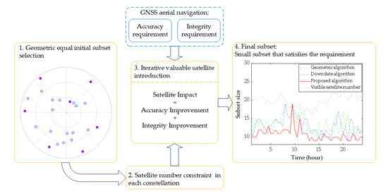
- A performance-requirement-driven fast satellite selection algorithm is raised according to the above investigation. It constructs the initial subset through geometric selection strategy to keep a tolerable accuracy and integrity, then improves the performance by adding a most valuable satellite to the subset until the required performance is met, thus a small size feasible subset is obtained.
As the GNSS is required to maintain the horizontal navigation safety during all phases of flight while the vertical navigation safety supported by GNSS is only required in approach and departure phases, as shown in Table 1. The satellite selection strategy takes horizontal accuracy and integrity as targets in this study while can also be applied to VPL-demanded flight phase through a similar process.
The rest of this paper is arranged as follows. Section 2 describes the accuracy and integrity models in the weighted slope-based RAIM algorithm and analyzes the impacts of subset size on the performance to exhibit the importance of satellite selection in the RAIM process. In Section 3, the impacts of a single satellite on the accuracy and integrity of the subset are investigated to recognize the valuable satellite for the current subset, then the performance-requirement-driven fast satellite selection algorithm is proposed according to the above investigation. Then, Section 4 illustrates the performance of the proposed algorithm with comparison simulations. Finally, the conclusion is drawn in Section 5.
2. Problem Statement
In this section, the accuracy and integrity models in the weighted slope-based RAIM algorithm is introduced at first. Then, we analyze the impacts of subset size on the accuracy and integrity performance through a scenario assumption way to exhibit the importance of satellite selection in the RAIM process.
2.1. Accuracy and Integrity Models in Weighted Slope-Based RAIM Algorithm
2.1.1. Accuracy Model
The linearized form of pseudo-range measurements model for GNSS can be described as [36]:
where is the measurement vector in the form of increment to the pseudo-range between satellites and receiver. is the number of satellites in use and is the constellation number plus three. is the states vector which involves increments to three components of receiver position and the clock offsets between constellations and the receiver. is the observation matrix in the local navigation frame and is the measurement error vector produced by receiver noise, wave propagation, satellite clock offsets, and possibly unexpected errors caused by failures to the assumption of normal-distributed noises or a satellite malfunction. The model of measurement error corresponding to each satellite is described later in Section 4.
When the accuracy of the pseudo-range measurements is known to differ, for example, due to variation in the carrier power to noise density or the residual ionosphere and troposphere propagation errors, which mainly depend on the elevation angle, a weighted least-squares estimate can be computed iteratively:
where is the inverse of the covariance matrix of the measurement error vector. For simplification, the error sources for each satellite are assumed to be uncorrelated with that for any other satellite. Therefore, all off-diagonal elements are set to zero and the diagonal elements are the inverses of the variances corresponding to each satellite.
The covariance of the estimated states vector can be expressed as:
Thus, the accuracy of that least-squares solution is mainly decided by two factors: the quality of the measurements, i.e., , and the satellite geometry which is described by observation matrix .
The horizontal accuracy of the navigation solution can be represented by the radius of the circle assured to contain the indicated horizontal position with a 95% probability under fault-free conditions [37]. It can be approximated by the two times distance root mean square (2drms) [10]
If the measurement errors are assumed to be independent and identically distributed with zero mean and variance , the horizontal accuracy of the navigation solution can be simplified as:
where the horizontal dilution of precision (HDOP) describes the satellite geometry factor of the horizontal accuracy and is defined as:
2.1.2. Integrity Model
If the weighted least-squares RAIM process is employed under the single fault hypothesis scenario, the integrity performance of the navigation solution can be evaluated by the protection level which represents the upper bound of the position error under a given reliability assumption if no alert. The horizontal protection level (HPL) is the protection level in the horizontal direction and can be determined by projecting the minimum detectable error from the measurement domain to the position domain [37]:
The in Equation (8) is the minimum detectable error under a given missed detection rate assumption in the measurement domain. It is not relevant to the satellite geometry and can be calculated according to the given integrity requirement and satellite number in use [19]. is the max slope of the satellites which will be used in the positioning process. The slope here means the sensitivity of the horizontal position error to the bias in each pseudo-range measurement and is defined as:
where:
As we can see, the HPL is highly correlated with the observation matrix . If a proper satellite geometry is constructed to minimize the max slope of the satellite subset, a lower HPL value will be obtained which means the positioning error can be constrained in a small region with the given reliability. By comparing the current HPL value with the horizontal alert limit (HAL) announced by the flight phase as in Table 1, the RAIM processor can determine whether the navigation system is suitable for the route segment.
2.2. Impacts of Subset Size on Accuracy and Integrity Performances
Although it is commonly believed that more satellites in view are considered and the more accurate and reliable solution will be achieved under fault-free conditions, the performance improvement caused by the satellite increase might be not always worthy of the increased channel and computation capability demand caused by that. Thus, it is necessary to investigate the relationship between subset size growth and its performance improvement and load increase effect.
2.2.1. Accuracy Performance Improved by Subset Size Growth
When the accuracy of the pseudo-range measurements is known to differ, it is uneasy to find a common configuration of the satellite geometry that can reach the smallest 2drms of the least-squares solution. In this situation, assuming the measurement errors are independent and identically distributed is an effective way to investigate the highest accuracy in each subset size. Thus, two simulation scenes are considered to illustrate the accuracy performance improved by subset size growth.
The first one brute force searches all the possible ideal satellite geometries above the mask angle of 5 degrees for each subset size under independent and identical measurement error assumption. Then it finds the subset with the highest accuracy, i.e., the smallest 2drms value in each given subset size. In fact, the high accuracy geometries for different size subsets have similar distributions that the satellites equally spaced on the low elevation bottom of the visible area. However, for the benefit of vertical accuracy performance, several satellites should be at the zenith of the sky [31]. Take the single constellation navigation system, for example, an observation matrix for the ideal subset with satellites can be summarized as:
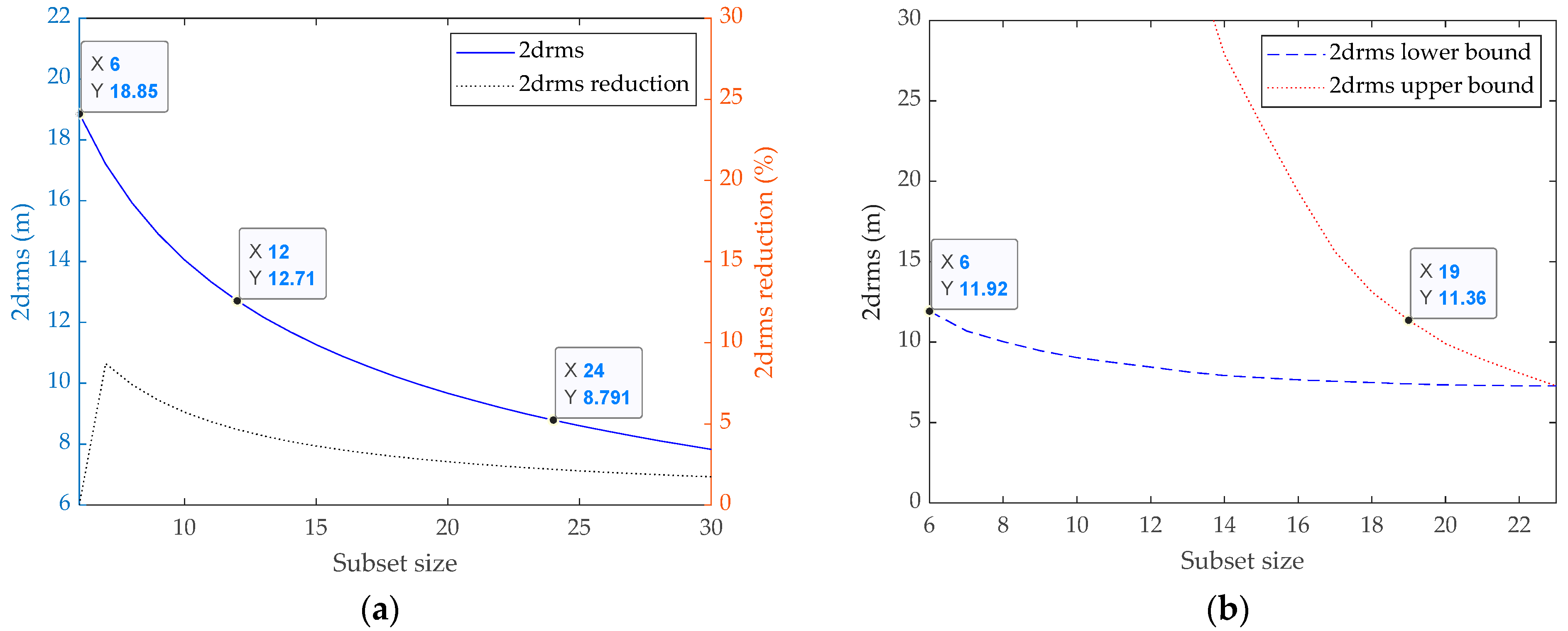
where is the satellite number at the zenith and is the mask angle. to are the elevation angles of satellites at the zenith and to are the azimuth angles of the zenith satellites. The minimal 2drms values for different size subsets can be found in Figure 1a when and the is set to 1 in this study. It is no doubt that the minimal 2drms value is decreased when more satellites are considered in the subset, as a better geometry can be structured. However, the improvement becomes less obvious when more satellites have been considered in the former. For example, if we need to reach a 2drms value of about 30% smaller than the 18.85 m in the 6 satellites subset, we should at least choose 12 satellites. However, if we need to reach a 2drms value of about 30% better than the 12 satellites subset, at least 24 satellites should be in the subset. In another word, if sufficient satellites have been used to achieve an acceptable accuracy, it is inefficient to improve the navigation accuracy by simply considering more satellites in the subset. The curve of 2drms reduction to the former subset in Figure 1a also supports this conclusion.
The second scene turns to a practical satellite distribution which includes 23 visible satellites from the GPS and the BeiDou satellite navigation system (BDS-2). The differences between pseudo-range measurement errors are taken into consideration and the accuracy varying range for each given size subset is shown in Figure 1b in the form of upper and lower bounds. As illustrated in the figure, the 2drms value of a given size subset can vary in a wide range, especially when only a small part of the all-in-view satellites is chosen. Additionally, we can notice that the 6 satellites subset can reach a 2drms value of 11.92 m if properly chosen, while the randomly chosen subset can maintain a better performance only if the subset size increases to 19 or larger. This means, the properly constructed subset can achieve a significantly better accuracy compared with the randomly chosen subset, even when the later owns more satellites. This verifies the importance of a good satellite selection method during the positioning process.
2.2.2. Integrity Performance Improved by Subset Size Growth
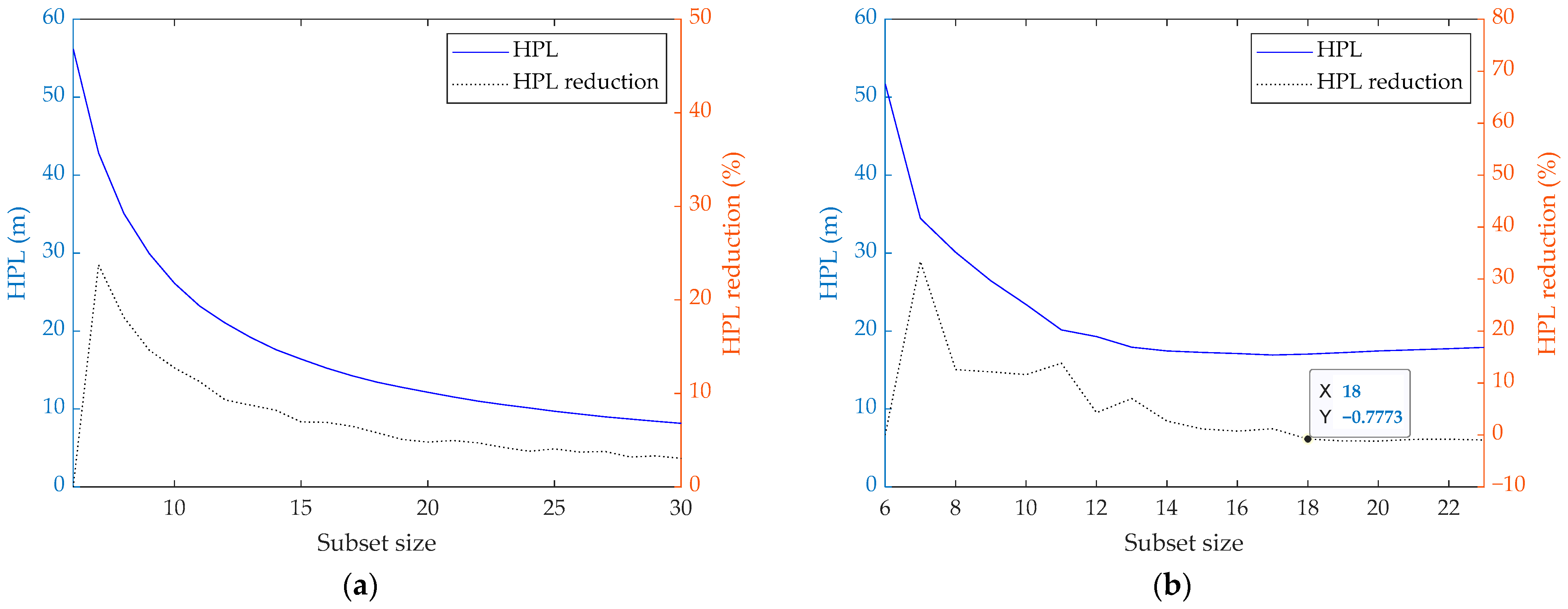
A similar scenario assumption way is used for the integrity performance analyses in different subset sizes. The ideal minimal HPL geometry is obtained when each satellite at the low elevation bottom circle has the same slope value, which means they are equally spaced on the low elevation bottom of the visible area under independent and identical measurement error assumption. The practical minimal HPL is gained through brute force searching all the possible subsets in the practical satellite distribution scene in which the pseudo-range measurement errors are known to differ. The results are also shown in Figure 2a and Figure 2b, separately.
A similar tendency can be observed in the ideal scene that the HPL value reduced by considering more satellites in the subset becomes unnoticeable as the subset size increases. What is more, an abnormal tendency is noticed in Figure 2b when the subset size reaches 18 and more. The minimal HPL value begins to increase not reduce even when more satellites are introduced. (Similar anomaly is also observed for VPLs in [23,25].) This conflicts with the intuition that the more satellites are considered, the better performance can be achieved, and further emphasize the importance of satellite selection in the RAIM process.
2.2.3. Computation Load Increased by Subset Size Growth
It is commonly known that the acquisition and tracking of the signal in space play an important role in the processing burden of the GNSS receiver. This burden grows proportionally as the satellites in use increase. Besides this, the computation load for RAIM process is discussed in this section.
If the weighted least-squares estimation algorithm is adopted to calculate the receiver position and clock offset, the estimation of the states vector can be expressed as Equation (2) and the HPL of the weighted RAIM process can be obtained by Equation (8). The amount of calculation for positioning and integrity monitoring can be given in Table 2. The multiplication and addition times for the inverse operation of only depend on the state dimension , thus the time complexity of the RAIM process is positively associated with the square of the satellite number . When the satellite number increases, the amount of extra operations for RAIM process increases more quickly than that for acquisition and tracking processes. Consequently, choosing a relatively small subset that meets the accuracy and integrity requirements is an efficient way to improve the real-time processing capability of the navigation processor.
Usually, the satellite selection method assigns a fixed subset size to maintain real-time processing capability. For example, the subset size is set to 8 for the dual-constellation navigation system and 10 for triple-constellation in [38], while 12 for the dual-constellation navigation system in [31,39], and 18 for the quadruple-constellation navigation system in [23]. However, the optimal performance of the same size subset varies with the satellite geometry which depends on the receiver location and time. Even in a specified location, the minimal geometric dilution of precision (GDOP) value of the 6 satellites subset can vary from 1.7 to 3.1 during 24 h as illustrated in [24], and the optimal HPL value of the 12 satellites subset varies between 13 and 20 m during 24 h in [31]. While maintaining reliable accuracy and integrity performances under the requirement, the minimal size of the usable subset will also not be a fixed number but vary with the satellite geometry and the satellite selection algorithm. The minimal subset size could be an indicator to evaluate the performance of the satellite selection strategy when we focus on the real-time processing capability of the navigation system.
3. Methodology
This section investigates the impacts of a newly introduced satellite on the accuracy and integrity of the subset to recognize the valuable satellite for the current subset, then the performance-requirement-driven fast satellite selection algorithm can be proposed according to the investigation.
3.1. Impacts of Single Satellite on the Accuracy and Integrity of Subset
In the minimal size satellite subset which we pursue, each satellite should hold an important place in the accuracy or integrity of the subset, otherwise, it could be removed without great effect on the performance of the subset. In another word, the satellite which greatly improves the accuracy or HPL of the subset when it is introduced is quite likely to be a member of the minimal size satellite subset. This assumption has also been employed by [25,32]. However, different from abounding less impact satellites from the all-in-view solution, this study tries to iteratively adding important satellite to the current subset so that a performance-requirement-satisfied subset can be efficiently constructed. In any event, evaluations on the accuracy and HPL effects of a single satellite are necessary for the satellite selection strategy.
3.1.1. Impact of Single Satellite on the Accuracy of Subset
Generally, the accuracy of the satellite subset will always be improved if the new valid satellite information is introduced. The accuracy effect of a single satellite on the subset can be represented by the HDOP value reduced by its inclusion as in Equation (12) and has been used in [7,27,40]. Although it is used for evaluating the accuracy effect of a single satellite on the all-in-view subset in the references, it is modified here to show the accuracy effect of a single satellite on the in-progress subset which needs the introduction of a new satellite.
The is the HDOP associated with the subset before the -th satellite is introduced and is the HDOP after that. (Note that the two notations here have different meanings from those in the reference). The HDOP effect is positive and is also derived in [41] as:
where . Multiply each side of Equations (12) and (13) by variance , then we can get:
If the measurement errors for each satellite are independent and identically distributed with zero mean and variance , i.e., , according to Equations (6) and (9) we can derive that:
where is the accuracy associated with the subset before the -th satellite is introduced and is the accuracy after that.
Although it is not theoretically derived in this study, simulation results show that the inference in Equation (15) still work when the accuracy of the pseudo-range measurements is known to differ. This finally reveals the connection between the accuracy effect of a satellite and its slope. As the slope means the sensitivity of the horizontal position error to the bias in each pseudo-range measurement. If the slope is large, which means the positioning accuracy is susceptible to the error in the corresponding satellite measurement, then the satellite has a large impact on the horizontal positioning accuracy of the navigation system.
As a result, the slope of a satellite can be a good mark of its accuracy importance. If each of the satellite in the subset has a large slope value, this subset may own a better horizontal accuracy performance than other same size subsets.
3.1.2. Impact of Single Satellite on the Integrity of Subset
According to the slope-based RAIM algorithm mentioned above, the HPL is proportional to the max slope value of the subset. When a small HPL is required, the slope of each satellite in the subset should also be limited in a small range. Similarly, an increment is introduced to demonstrate the contribution of a single satellite on the integrity of the subset.
The in Equation (16) is the max slope of the subset before the -th satellite is introduced, and is the new max slope of the subset after that.
If the newly introduced satellite always owns positive value, which means the max slope value is reduced in each iteration, then the HPL performance can keep improving as the subset size increases. However, this strategy may be obstructed as the abnormal tendency shown in Figure 2b when the added satellite not reduces but increases the slope of the former max slope satellite [42]. Fortunately, this abnormal tendency occurs in the satellite selection strategy mostly when the visible satellite number is very large and the subset size is close to the all-in-view subset thus is not so critical in this study.
3.1.3. Integrated Performance Impact of Single Satellite
As discussed in the above paragraphs, a larger slope value of a single satellite means a greater accuracy impact it has, but a too-large slope value is disadvantageous for the integrity of the subset and a new satellite may be required to reduce it. As the purpose of this study is to find a relatively small subset that satisfies the accuracy and integrity requirements, the gap between the required performance and the performance of the current subset can be employed to help decide which satellite is more valuable.
A cost function is constructed to represent the integrated performance impact of a newly added satellite as:
The in Equation (17) is the integrated performance impact of the new satellite. The is the accuracy requirement and the is the max slope requirement derived from the required HPL. The is the slope of the new satellite after its introduction. It is easy to derive from Equation (17) that, if the performance requirement is given, the integrated performance impact of a single satellite mainly depends on its slope in the new subset and the max slope of the new subset after its introduction. When a new satellite owns a larger slope value and more greatly reduce the max slope of the subset, it makes a greater integrated performance impact and thus more suitable for the current subset to efficiently achieves the required performance.
If the navigation system is not aware of the performance requirement, the value of and in Equation (17) can be replaced by zero. Then the turns to the sum of the slope reduction rate and accuracy reduction rate of the new satellite. Nevertheless, it can still be a reference to the integrated performance impact of the satellite.
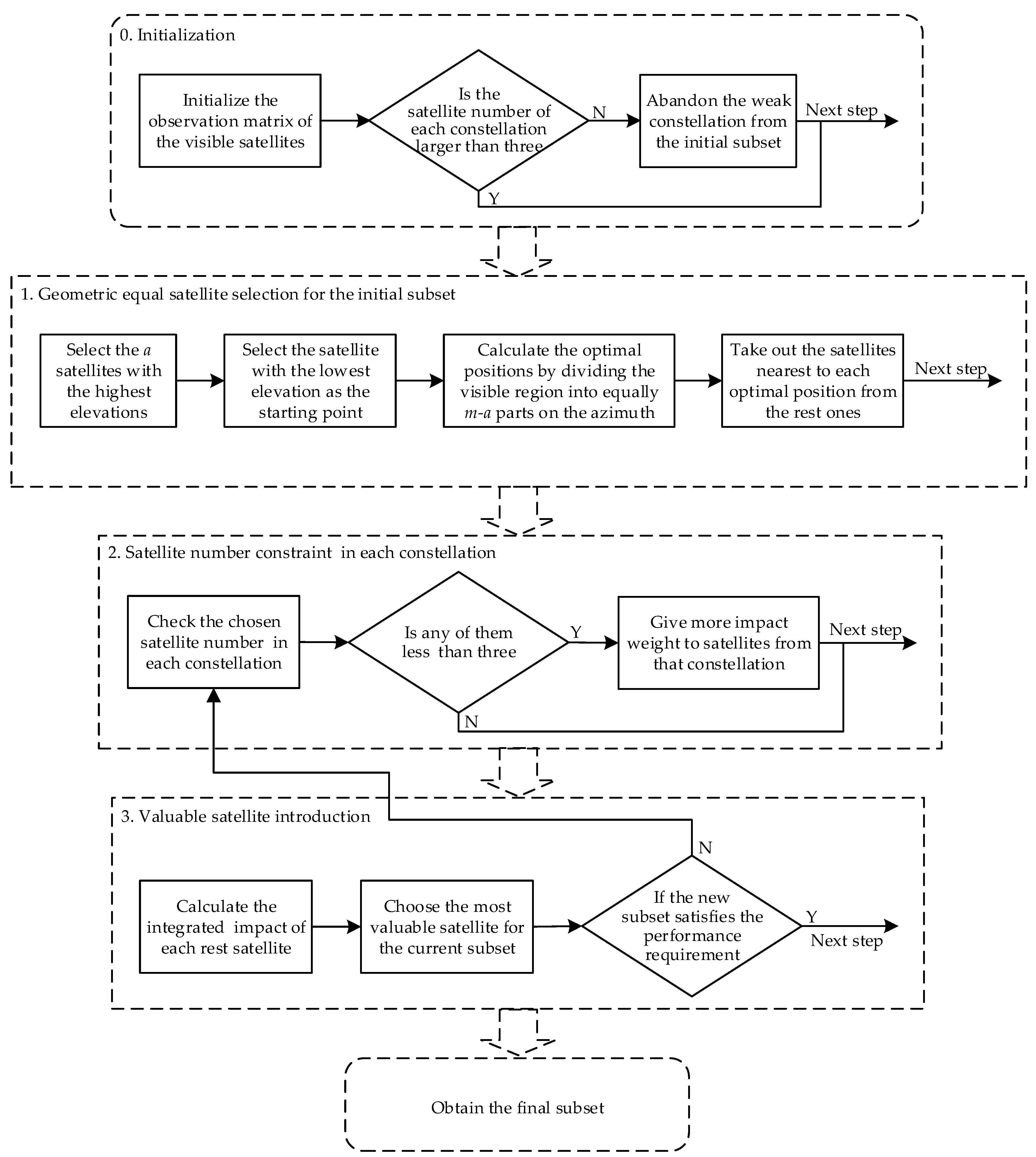
3.2. Performance-Requirement-Driven Fast Satellite Selection Algorithm
According to the performance impact analyses in Section 3.1, a performance-requirement-driven fast satellite selection (PRDFSS) algorithm can be carried out to construct a relatively small subset that satisfies both the accuracy and integrity requirements. The main idea of the algorithm is constructing a small size initial subset through a geometric selection strategy, then improving the performance by adding the valuable satellite to the subset sequentially until the required performance is reached, thus a small feasible subset is obtained.
The proposed PRDFSS algorithm is comprised of three parts which are illustrated as follows:
3.2.1. Geometric Equal Satellite Selection for the Initial Subset
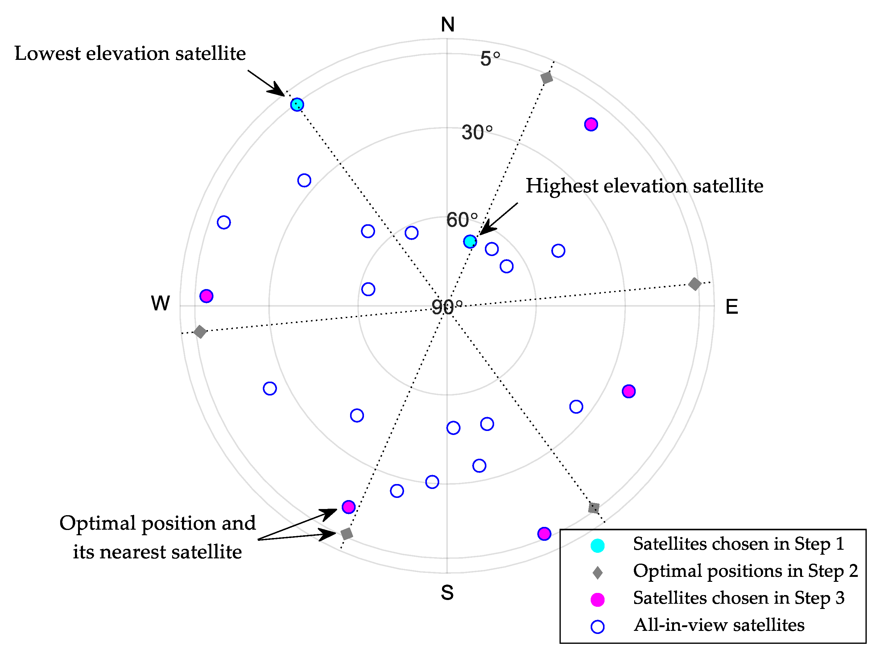
As mentioned in Section 2.2.1 and Section 2.2.2, If the measurement errors are assumed to be independent and identically distributed, the ideal minimal 2drms and HPL geometries have a similar distribution that the satellites with low elevations equally spaced at the low elevation bottom of the visible area, the subset can be constructed by geometric equally selecting the satellites so that an appropriate geometry can be formed and the relatively small accuracy and max slope values can be guaranteed. This principle has been used for HDOP-based satellite selection but is utilized for initial subset construction here. An example for initial subset selection is shown in Figure 3.
The specific steps for initial subset selection can be summarized as:
- Selecting the first satellites with the highest elevations then selecting the satellite with the lowest elevation as the starting point of the region partition process in the next step. The chosen satellites are shown as the light cyan points in Figure 3;
- Calculating the optimal positions by dividing the visible region into equally parts on the azimuth from the starting point selected in the previous step. The optimal positions are shown as the grey diamond points in Figure 3;
- Taking out the satellites nearest to each optimal position sequentially from the rest ones, as the manganese violet points in Figure 3. Therefore, the first satellites are selected.
3.2.2. Satellite Number Constraint in Each Constellation
In the multi-constellation system, extra measurements are needed to estimate the clock offset for each constellation. A special situation that only one satellite from a secondary constellation is included in the subset is helpless for the performance of the subset. As the single satellite is essential for the estimation of the clock offset between the receiver and its constellation, it provides little or even negative contribution to the accuracy of the subset but has a crucial impact on the state estimation result thus is hazardous for the integrity of the system. This situation should be avoided during the satellite selection process. A suggested configuration is that more than three satellites from each constellation are retained, or the insignificant constellation is abandoned in the final subset [31].
In this algorithm, the abandonment operation is checked and executed in the initialization step. The satellite number constraint process is executed accompany by the valuable satellite introduction process. If the satellite number from any constellation in the current subset is less than three and the visible satellite number of that constellation is more than three, then the alternative satellites from that constellation will gain more weights when comparing their integrated performance impacts.
3.2.3. Valuable Satellite Introduction
After the alternative set is confirmed, the valuable satellite can be selected from the set by the cost function raised above. The integrated impact of each satellite in the alternative set is calculated and the one with the largest impact on the current subset is chosen as the added satellite in this iteration. When the accuracy and integrity requirements are both satisfied in the current subset, the iteration ends and the required subset is obtained.
The schematic overview of the PRDFSS algorithm is illustrated in Figure 4. As the geometric equal satellite selection part is executed only based on the geometric position of each satellite, no matrix inversion operation is needed. Additionally, the execution times of the slope calculation operation in each iteration is no more than the number of rest satellites, so the computation load is significantly lighter than that of the brute force searching method and similar with that of the greedy method.
4. Results and Discussion
In this section, simulations are carried out to investigate the performance of the proposed PRDFSS algorithm. The satellite navigation data are obtained from the HWA-RNSS-7400 satellite navigation signal simulator and the GPS/BDS-2 dual-constellation single-frequency navigation system is employed to provide the satellite signals for positioning and RAIM process. The receiver is placed in a suburb of Xi’an (N34.45°, E108.75°, 480 m). It remains stationary while continuously acquiring and tracking visible satellite signals during the simulations. The simulations begin from 00:00 UTC on 10th March 2021 and last for 24 h. The satellite selection operation is executed every half an hour and the performances of the final subsets chosen by different strategies are evaluated. An Intel Core i7-7700HQ CPU @ 2.80 GHz with 16 GB RAM is used as simulation hardware for computation load comparison.
The variances of measurement error corresponding to each satellite are composed of the following factors during the simulations.
where is the standard deviation of satellite pseudo-range measurement, is the standard deviation of clock/ephemeris error, is the ionospheric delay estimation error, is the tropospheric delay estimation error, is the standard deviation of the multipath and receiver noise modeled as a Gaussian white sequence with samples that are uncorrelated in time.
With the receiver independent exchange format (RINEX) GNSS navigation message files, the user range accuracy (URA) information and parameters for ionospheric correction in GPS constellation and BDS-2 constellation are extracted, respectively. The Klobuchar ionospheric delay model is used for GPS and BDS-2 but with different parameters. The Saastamoinen troposphere delay model is used for tropospheric delay estimation in this paper.
The three comparison trials are set up for performance evaluation on the satellite selection algorithms include the HDOP-based geometric equal satellite selection algorithm (geometric algorithm for short) as in [23,31], the HPL-based downdate satellite selection algorithm (downdate algorithm for short) in [25], and the PRDFSS algorithm proposed in this study. As mentioned in Section 1 and Section 3.2.1, the geometric algorithm uses the selection strategy that approximate geometric equally selecting the satellites at the low elevation bottom of the visible area. The downdate algorithm uses the measurements (in some way like the slopes of satellites in the all-in-view subset) as impact values of each satellite and retains the several satellites with the largest impact values to construct a superior subset.
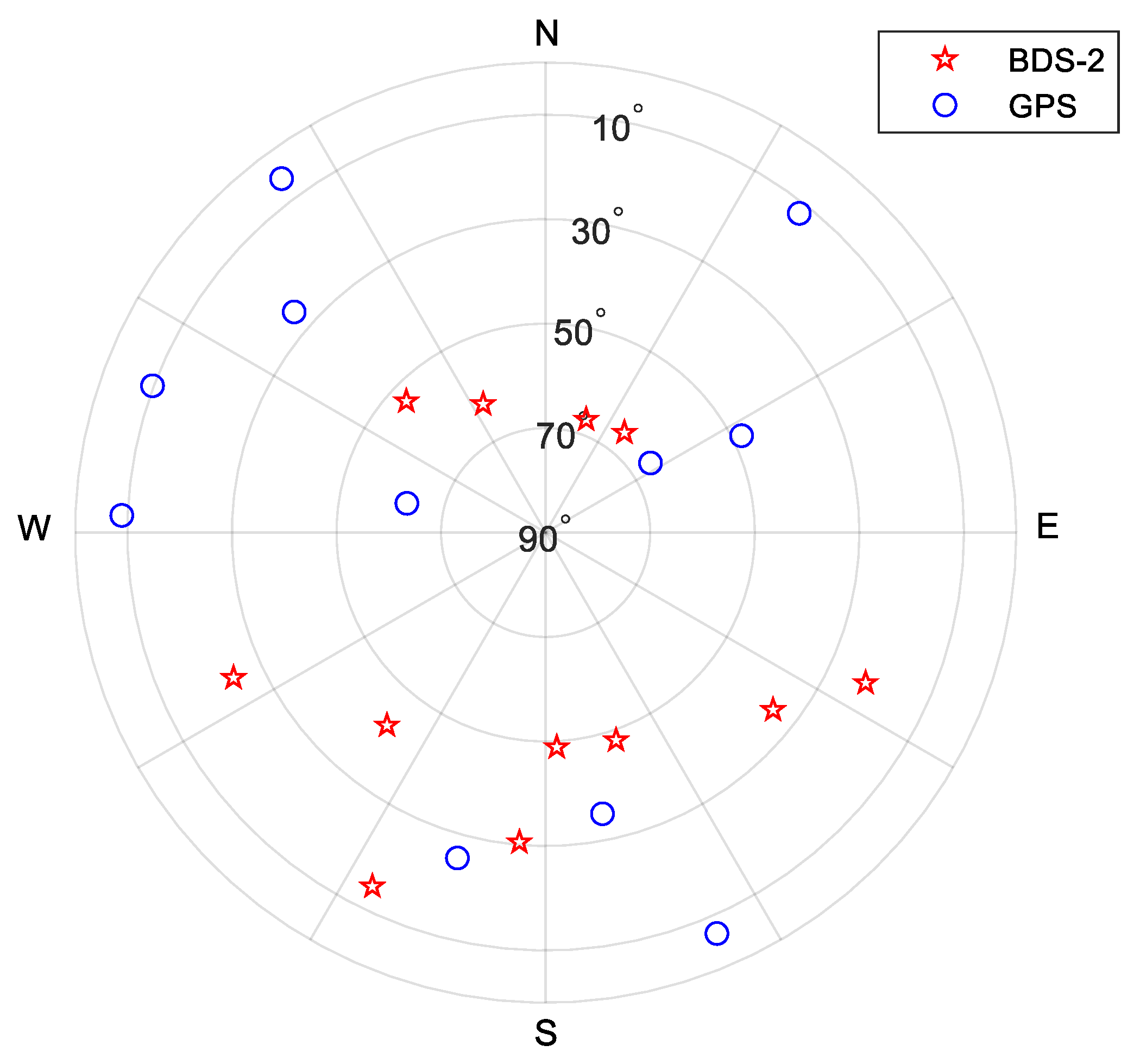
In the first trial, the final subset size is fixed to 12 for the dual-constellation satellite selection strategies. The accuracy, integrity and computation load are compared among the three algorithms. The sky plot view of the satellite geometry at the beginning of the trial is shown in Figure 5.
In the second trial, general requirements for the Lateral Navigation (LNAV) operation [43], as shown in Table 3, and the horizontal requirements for approach procedures with vertical guidance (APV-I) operation as in Table 1 are used to analyze the minimal subset choosing ability of the proposed algorithm.
In the third trial, the former two simulations are carried out in the Mohe Gulian Airport (N52.92°, E122.43°, 296 m) to evaluate the performance of the satellite selection strategies in the high latitudes.
4.1. Fixed Subset Size Simulations
In this trial, the cost function of proposed satellite selection algorithm is constructed by the sum of accuracy and integrity impacts instead of driven by the performance requirement, so that it can be used for fixed number satellite selection.
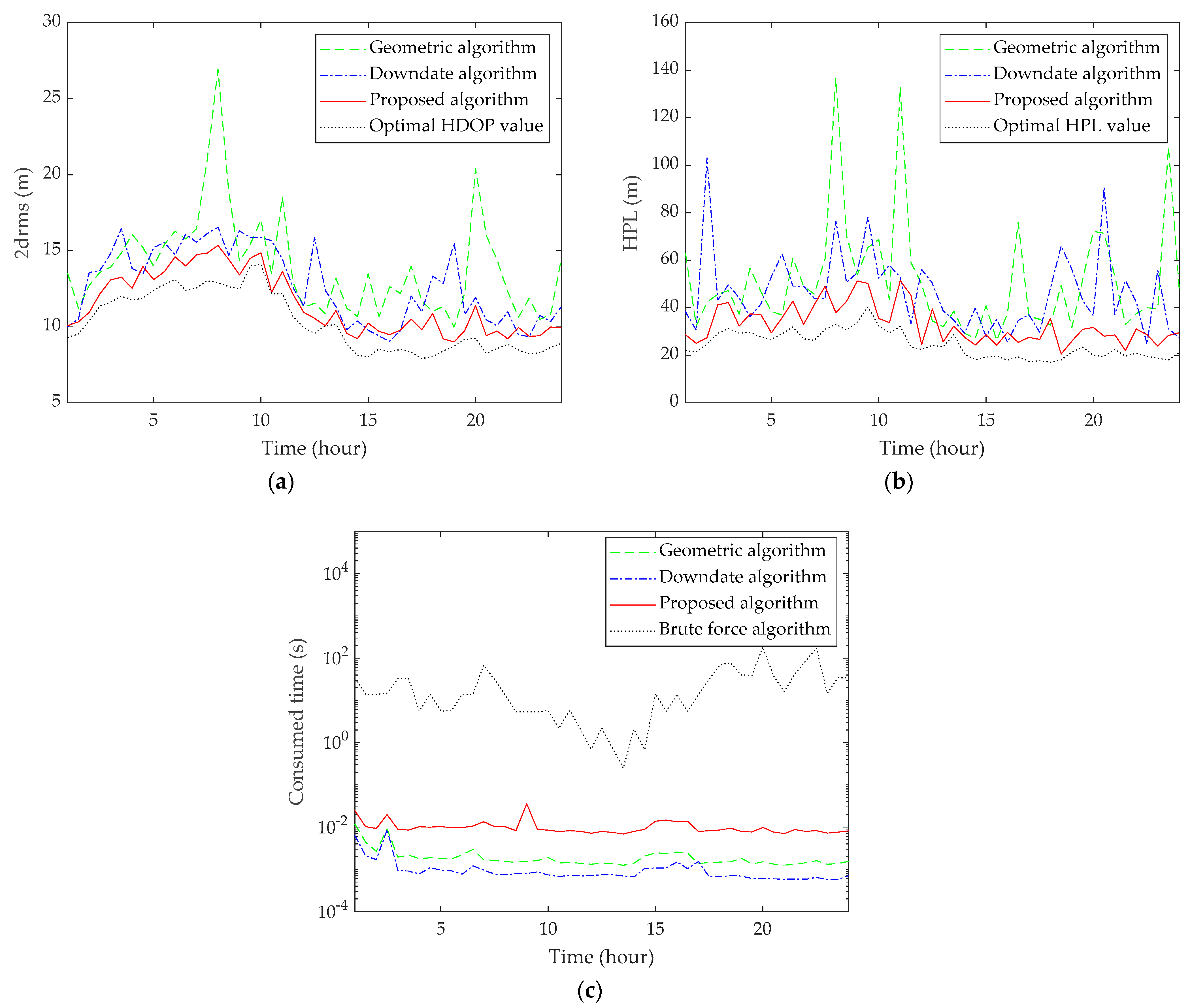
The accuracy and HPL of the subset selected by each satellite selection algorithm during the simulation are shown in Figure 6a,b separately and the consumed time of each algorithm is shown in Figure 6c. The average 2drms, HPL and consumed time of each algorithm are listed in Table 4.
All the three algorithms can obtain good accuracy performance which is well below 28 m when 12 satellites are selected in the dual-constellation navigation system. The downdate algorithm can obtain a little smaller 2drms than the geometric algorithm as the large slope satellites which have great accuracy impacts are chosen as a priority. Additionally, the proposed algorithm can reach a bit better accuracy performance than the downdate algorithm and is close to the optimal 2drms value. As for the integrity performance, the geometric algorithm and the downdate algorithm reach similar HPLs, with an average of about 48 to 52 m, but the HPL of the geometric algorithm fluctuates more strongly. While the proposed algorithm performs best among the three with an average HPL value of about 33 m, as the integrity impacts of alternative satellites are taken into consideration. The consumed times of the geometric algorithm and the downdate algorithm are well below 0.01 s and the proposed algorithm takes a little longer time with an average of about 0.012 s. However, all of them are significantly efficient than the brute force algorithm.
4.2. Minimal Subset Size Simulations
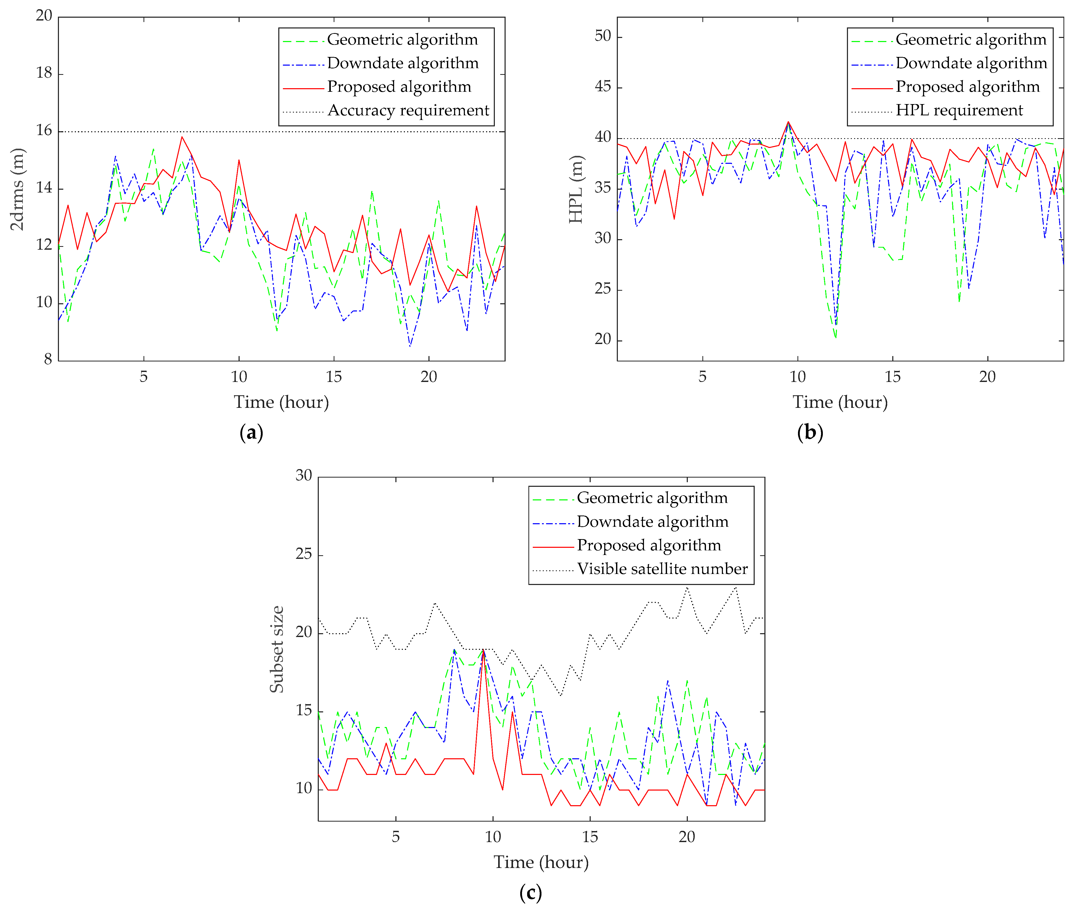
In this trial, performance requirement constraints are added to the geometric algorithm and the downdate algorithm so that they can be used to search for the minimal subset which satisfies the requirement. Firstly, the LNAV performance requirement is considered to check if it can be met by the dual-constellation navigation system. The 2drms, HPL and subset size of the final subset constructed by each algorithm during the simulation are illustrated in Figure 7. As the final subset size in each algorithm is well below the visible satellite number during the simulation, this means the LNAV requirements can be well satisfied by the GPS/BDS-2 single-frequency navigation system. Among the three satellite selection strategies, the proposed algorithm reaches the smallest final subset size with an average value of 6.54, about 1.00 smaller than that of the geometric algorithm and 1.54 smaller than that of the downdate algorithm, at a cost of little increased 2drms value that still within the requirement. The average consumed times of these algorithms are close and all less than 0.01 s.
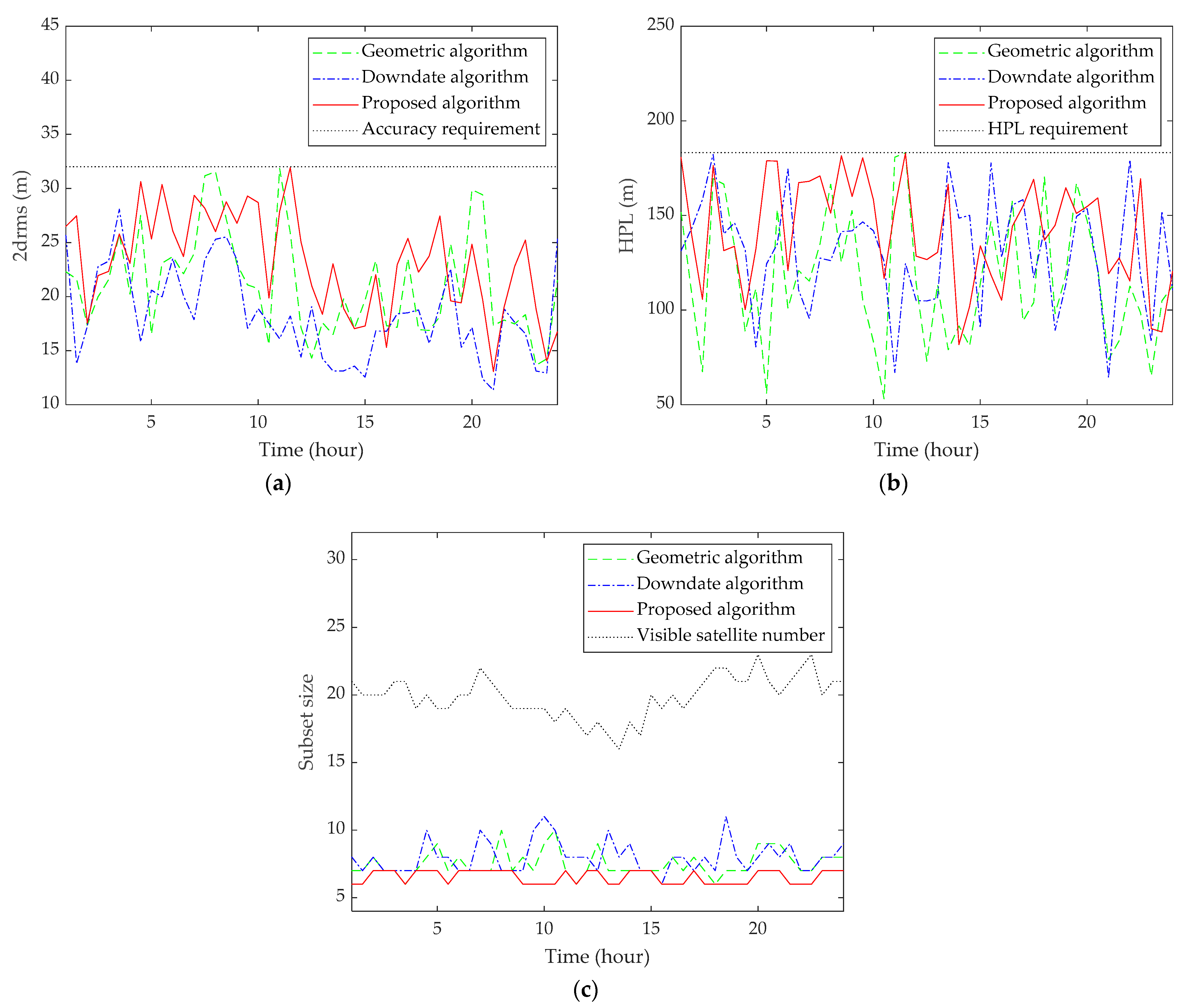
Secondly, the horizontal requirement of APV-I is utilized here to analyze the capability of the GPS/BDS-2 single-frequency navigation system in aerial navigation. The 2drms, HPL and subset size of the final subset constructed by each algorithm are illustrated in Figure 8. As we can see, the accuracy requirement is satisfied by the three algorithms during the simulation. However, the integrity requirement is violated by them during the 9–10 h. The final subsets at these times all reach the all-in-view subset but still cannot entirely meet the requirements for not enough satellites in view or poor geometries. However, the curves in Figure 8c show that the proposed algorithm can maintain a relatively smaller subset during the simulation, with an average subset size of 10.77, which is 3.02 smaller than that of the geometric algorithm and 2.54 smaller than that of the downdate algorithm. Additionally, the three algorithms reach similar average consumed time, as shown in Table 5.
4.3. High Latitudes Simulations
To verify the effectiveness of the satellite selection algorithms in different locations, especially in high latitudes, the receiver is moved to the Mohe Gulian Airport whose latitude is higher than 50 degrees in the north. The simulations in the fix subset size scene and minimal subset size scene are carried out in sequence and the 24-h statistical results are summarized in Table 6. During the 12 satellite subset trial, the three algorithms reach similar accuracy performance while the proposed algorithm outperforms the other two in integrity with an average 15 to 27 m smaller HPL. During the LNAV and APV-I requirement trial, the LNAV requirement is well met by the three algorithms and the proposed algorithm obtains an average 1.31 smaller subset. The APV-I integrity requirement is violated by the three algorithms over a period of time, which means the GPS/BDS-2 single-frequency navigation system alone may not be suitable for the APV-I operation. Even so, the proposed algorithm obtains an average 2.06 to 3.63 smaller subset beyond these discordant time.
As a result, the proposed PRDFSS algorithm performs well on both accuracy and integrity performances regardless of fixed subset size trial or minimal subset size trial. When 12 satellites are selected in the GPS/BDS-2 navigation system, the proposed algorithm can reach a comparable 2drms and an about 15 m lower HPL than the geometric algorithm and the downdate algorithm. When the LNAV and APV-I performance is required, an average 1.3 to 2.0 satellites smaller subset can be achieved by the proposed algorithm if compared with the other two, regardless of the latitude of the receiver. Besides, the average consumed times of the three algorithms are very close and short, so the proposed PRDFSS algorithm is suitable for performance-requirement-based navigation applications with limited real-time processing capability.
5. Conclusions
The significant increase in operating satellites in view turns out not only a benefit for the positioning accuracy but also a challenge to the processing capability of the general civil low-cost navigation device, as well as the channel limitation of the GNSS receiver processor. This study investigates the importance of satellite selection in the multi-constellation navigation system then proposed a performance-requirement-driven fast satellite selection algorithm in order to find a relatively small subset that meets the requirements for the RAIM applications.
The investigations about subset size impacts on the accuracy, integrity, and computation load show that, it may be not the more selected satellites the better for the RAIM process and satellite selection is quite effective when real-time requirement and channel capabilities are considered. The accuracy impact of a single satellite can be represented by its slope on the current subset while the integrity impact is indicated by the max slope value it reduces. A cost function based on the performance requirement can help to select a valuable satellite for the current subset. A performance-requirement-driven fast satellite selection algorithm is raised by geometric evenly selecting the initial subset and adding valuable satellites iteratively to the initial subset until the performance requirement is achieved. The proposed algorithm keeps a similar accuracy performance and an about 15 m smaller horizontal protection level than the geometric algorithm and the downdate algorithm in the 12-satellite subset trial and can achieve an average 1.0 to 2.0 satellites smaller subset than the other two algorithms under the given LNAV and APV-I horizontal requirements, regardless of the latitude of the receiver. Consequently, it could be a good choice for real-time RAIM applications and low-cost navigation devices.
Author Contributions
Conceptualization, H.W.; Methodology, S.L. and Z.L.; Supervision, Y.C. and C.C.; Writing—original draft, H.W.; Writing—review and editing, Y.C., C.C., S.L. and Z.L. All authors have read and agreed to the published version of the manuscript.
Funding
This work was supported in part by the National Natural Science Foundation of China under Grant 61901380 and in part by the Stable Supporting Fund of National Key Laboratory on Blind Signal Processing under Grant 61424131903.
Institutional Review Board Statement
Not applicable.
Informed Consent Statement
Not applicable.
Data Availability Statement
The data presented in this study are available on request from the corresponding author.
Conflicts of Interest
The authors declare no conflict of interest.
References
- ICAO. Doc 9613, Performance-Based Navigation (PBN) Manual, 4th ed.; ICAO: Montreal, QC, Canada, 2013. [Google Scholar]
- RTCA, Inc. Minimum Aviation System Performance Standards: Required Navigation Performance for Area Navigation; RTCA DO-236B; RTCA: Washington, DC, USA, 2003; pp. 21–24. [Google Scholar]
- Ochieng, W.Y.; Sauer, K.; Walsh, D.; Brodin, G.; Griffin, S.; Denney, M. GPS integrity and potential impact on aviation safety. J. Navig. 2003, 56, 51. [Google Scholar] [CrossRef]
- Nowel, K.; Cellmer, S.; Fischer, A. Validation of GNSS baseline observation models using information criteria. Surv. Rev. 2020. [Google Scholar] [CrossRef]
- Krasuski, K.; Wierzbicki, D. Monitoring Aircraft Position Using EGNOS Data for the SBAS APV Approach to the Landing Procedure. Sensors 2020, 20, 1945. [Google Scholar] [CrossRef] [Green Version]
- Krasuski, K.; Cwiklak, J.; Grzegorzewski, M. Aircraft positioning using GPS/GLONASS code observations. Aircr. Eng. Aerosp. Technol. 2020, 92, 163–171. [Google Scholar] [CrossRef]
- Brown, R.G. A baseline GPS RAIM scheme and a note on the equivalence of three RAIM methods. Navigation 1992, 39, 301–316. [Google Scholar] [CrossRef]
- Bhattacharyya, S.; Gebre-Egziabher, D. Kalman filter–based RAIM for GNSS receivers. IEEE Trans. Aerosp. Electron. Syst. 2015, 51, 2444–2459. [Google Scholar] [CrossRef]
- Sun, Y. RAIM-NET: A Deep Neural Network for Receiver Autonomous Integrity Monitoring. Remote Sens. 2020, 12, 1503. [Google Scholar] [CrossRef]
- Walter, T.; Enge, P. Weighted RAIM for Precision Approach. In Proceedings of the 8th International Technical Meeting of the Satellite Division of The Institute of Navigation (ION GPS 1995), Palm Springs, CA, USA, 12–15 September 1995; pp. 1995–2004. [Google Scholar]
- Milner, C.D.; Ochieng, W.Y. Weighted RAIM for APV: The Ideal Protection Level. J. Navig. 2011, 64, 61–73. [Google Scholar] [CrossRef]
- Fu, L.; Zhang, J.; Li, R.; Cao, X.; Wang, J. Vision-Aided RAIM: A New Method for GPS Integrity Monitoring in Approach and Landing Phase. Sensors 2015, 15, 22854–22873. [Google Scholar] [CrossRef] [Green Version]
- Sabatini, R.; Moore, T.; Ramasamy, S. Global Navigation Satellite Systems Performance Analysis and Augmentation Strategies in Aviation. Prog. Aeosp. Sci. 2017, 95, 45–98. [Google Scholar] [CrossRef]
- Pan, W.; Zhan, X.; Zhang, X. Fault exclusion method for ARAIM based on tight GNSS/INS integration to achieve CAT-I approach. IET Radar Sonar Navig. 2019, 13, 1909–1917. [Google Scholar] [CrossRef]
- Yeh, S.J.; Jan, S.S. Operational Receiver Autonomous Integrity Monitoring Prediction System for Air Traffic Management System. J. Aircr. 2017, 54, 346–353. [Google Scholar] [CrossRef]
- Nowak, A. The Proposal to “Snapshot” Raim Method for Gnss Vessel Receivers Working in Poor Space Segment Geometry. Pol. Marit. Res. 2015, 22, 3–8. [Google Scholar] [CrossRef] [Green Version]
- Zalewski, P. Integrity Concept for Maritime Autonomous Surface Ships’ Position Sensors. Sensors 2020, 20, 2075. [Google Scholar] [CrossRef] [Green Version]
- Zalewski, P. GNSS Integrity Concepts for Maritime Users. In Proceedings of the 2019 European Navigation Conference (ENC), Warsaw, Poland, 9–12 April 2019; pp. 1–10. [Google Scholar] [CrossRef]
- Feng, S.; Ochieng, W.Y.; Walsh, D.; Ioannides, R. A measurement domain receiver autonomous integrity monitoring algorithm. GPS Solut. 2006, 10, 85–96. [Google Scholar] [CrossRef]
- Joerger, M.; Chan, F.C.; Pervan, B. Solution separation versus residual-based RAIM. Navigation 2014, 61, 273–291. [Google Scholar] [CrossRef]
- Ma, X.; Yu, K.; Montillet, J.P.; He, X. Equivalence Proof and Performance Analysis of Weighted Least Squares Residual Method and Weighted Parity Vector Method in RAIM. IEEE Access 2019, 7, 97803–97814. [Google Scholar] [CrossRef]
- Zhai, Y.; Joerger, M.; Pervan, B. Fault exclusion in multi-constellation global navigation satellite systems. J. Navig. 2018, 71, 1281–1298. [Google Scholar] [CrossRef]
- Luo, S.; Wang, L.; Tu, R.; Zhang, W.; Wei, J.; Chen, C. Satellite selection methods for multi-constellation advanced RAIM. Adv. Space Res. 2020, 65, 1503–1517. [Google Scholar] [CrossRef]
- Zhang, M.; Zhang, J. A fast satellite selection algorithm: Beyond four satellites. IEEE J. Sel. Top. Signal Process. 2009, 3, 740–747. [Google Scholar] [CrossRef]
- Walter, T.; Blanch, J.; Kropp, V. Satellite selection for multi-constellation SBAS. In Proceedings of the 29th International Technical Meeting of the Satellite Division of The Institute of Navigation (ION GNSS+ 2016), Portland, OR, USA, 12–16 September 2016; pp. 1350–1359. [Google Scholar] [CrossRef] [Green Version]
- Kihara, M.; Okada, T. A satellite selection method and accuracy for the global positioning system. Navigation 1984, 31, 8–20. [Google Scholar] [CrossRef]
- Phatak, M.S. Recursive method for optimum GPS satellite selection. IEEE Trans. Aerosp. Electron. Syst. 2001, 37, 751–754. [Google Scholar] [CrossRef]
- Meng, F.; Wang, S.; Zhu, B. GNSS reliability and positioning accuracy enhancement based on fast satellite selection algorithm and RAIM in multiconstellation. IEEE Aerosp. Electron. Syst. Mag. 2015, 30, 14–27. [Google Scholar] [CrossRef]
- Huang, P.; Rizos, C.; Roberts, C. Satellite selection with an end-to-end deep learning network. GPS Solut. 2018, 22, 108. [Google Scholar] [CrossRef]
- Du, H.; Hong, Y.; Xia, N.; Zhang, G.; Yu, Y.; Zhang, J. A Navigation Satellites Selection Method Based on ACO with Polarized Feedback. IEEE Access 2020, 8, 168246–168261. [Google Scholar] [CrossRef]
- Gerbeth, D.; Martini, I.; Rippl, M.; Felux, M. Satellite selection methodology for horizontal navigation and integrity algorithms. In Proceedings of the 29th International Technical Meeting of the Satellite Division of The Institute of Navigation (ION GNSS+ 2016), Portland, OR, USA, 12–16 September 2016; pp. 2789–2798. [Google Scholar] [CrossRef]
- Gerbeth, D.; Felux, M.; Circiu, M.S.; Caamano, M. Optimized selection of satellite subsets for a multi-constellation GBAS. In Proceedings of the 2016 International Technical Meeting of The Institute of Navigation, Monterey, CA, USA, 25–28 January 2016; pp. 360–367. [Google Scholar] [CrossRef] [Green Version]
- Gerbeth, D.; Caamano, M.; Circiu, M.S.; Felux, M. Satellite selection in the context of an operational GBAS. Navigation 2019, 66, 227–238. [Google Scholar] [CrossRef] [Green Version]
- Blanch, J.; Walter, T.; Enge, P.; Lee, Y.; Pervan, B.; Rippl, M.; Spletter, A. Advanced RAIM user algorithm description: Integrity support message processing, fault detection, exclusion, and protection level calculation. In Proceedings of the 2012 Global Navigation Satellite Systems Conference of the Institute of Navigation (ION GNSS 2012), Nashville, TN, USA, 17–21 September 2012; pp. 2828–2849. [Google Scholar]
- Blanch, J.; Walker, T.; Enge, P.; Lee, Y.; Pervan, B.; Rippl, M.; Spletter, A.; Kropp, V. Baseline advanced RAIM user algorithm and possible improvements. IEEE Trans. Aerosp. Electron. Syst. 2015, 51, 713–732. [Google Scholar] [CrossRef]
- Groves, P.D. Principles of GNSS, Inertial, and Multisensor Integrated Navigation Systems, 2nd ed.; Artech House: Boston, MA, USA, 2013; pp. 451–470. [Google Scholar]
- Kaplan, E.D.; Hegarty, C. Understanding GPS/GNSS: Principles and Applications, 3rd ed.; Artech House: Boston, MA, USA, 2017; pp. 661–730. [Google Scholar]
- Li, F.; Li, Z.; Gao, J.; Yao, Y. A Fast Rotating Partition Satellite Selection Algorithm Based on Equal Distribution of Sky. J. Navig. 2019, 72, 1053–1069. [Google Scholar] [CrossRef]
- Abedi, A.A.; Mosavi, M.R.; Mohammadi, K. A new recursive satellite selection method for multi-constellation GNSS. Surv. Rev. 2020, 52, 330–340. [Google Scholar] [CrossRef]
- Zhang, C.; Zhao, X.; Pang, C.; Zhang, L.; Feng, B. The influence of satellite configuration and fault duration time on the performance of fault detection in GNSS/INS integration. Sensors 2019, 19, 2147. [Google Scholar] [CrossRef] [Green Version]
- Sturza, M.A.; Brown, A.K. Comparison of fixed and variable threshold RAIM algorithms. In Proceedings of the 3rd International Technical Meeting of the Satellite Division of the Institute of Navigation (ION GPS 1990), Colorado Spring, CO, USA, 19–21 September 1990; pp. 437–443. [Google Scholar]
- Wang, H.; Cheng, Y.; Wei, X.; Li, S.; Wang, H.; Li, Z. A slope-based fast satellite selection algorithm for multi-constellation RAIM. In Proceedings of the 2020 Chinese Automation Congress (CAC 2020), Shanghai, China, 6–8 November 2020. [Google Scholar] [CrossRef]
- RTCA, Inc. Minimum Operational Performance Standards for GPS WAAS Airborne Equipment; RTCA DO-229D; RTCA: Washington, DC, USA, 2006; pp. 41–49. [Google Scholar]
Figure 1.
(a) Minimal 2drms value and 2drms reduction to the former for each size subset in the ideal scene; (b) Accuracy variation range for each size subset in the practical scene.
Figure 1.
(a) Minimal 2drms value and 2drms reduction to the former for each size subset in the ideal scene; (b) Accuracy variation range for each size subset in the practical scene.

Figure 2.
Minimal HPL value and HPL reduction to the former for each size subset. (a) In the ideal scene; (b) In the practical scene.
Figure 2.
Minimal HPL value and HPL reduction to the former for each size subset. (a) In the ideal scene; (b) In the practical scene.

Figure 3.
An example for initial subset selection when .

Figure 4.
Schematic overview of the PRDFSS algorithm.

Figure 5.
Sky plot view of the satellite geometry at the beginning of the trial.

Figure 6.
2drms and HPL of the subset and consumed time of each satellite selection algorithm in the fixed subset size trial. (a) 2drms value; (b) HPL value; (c) Consumed time.
Figure 6.
2drms and HPL of the subset and consumed time of each satellite selection algorithm in the fixed subset size trial. (a) 2drms value; (b) HPL value; (c) Consumed time.

Figure 7.
2drms, HPL and subset size of the final subset constructed by each algorithm under LNAV requirement. (a) 2drms value; (b) HPL value; (c) Subset size.
Figure 7.
2drms, HPL and subset size of the final subset constructed by each algorithm under LNAV requirement. (a) 2drms value; (b) HPL value; (c) Subset size.

Figure 8.
2drms, HPL and subset size of the final subset constructed by each algorithm under APV-I horizontal requirement. (a) 2drms value; (b) HPL value; (c) Subset size.
Figure 8.
2drms, HPL and subset size of the final subset constructed by each algorithm under APV-I horizontal requirement. (a) 2drms value; (b) HPL value; (c) Subset size.


Table 1.
Aviation GNSS signal-in-space performance requirements [13].
Table 1.
Aviation GNSS signal-in-space performance requirements [13].
| Type of Operation | HOR./VERT. Accuracy (95%) | Integrity | HAL/VAL | Time to Alert | Continuity | Availability |
|---|---|---|---|---|---|---|
| En Route Oceanic | 3700 m/NA | 1–10−7/h | 7408 m/NA | 5 min | 1–10−4/h to 1–10−8/h | 0.99 to 0.99999 |
| En Route Continental | 3700 m/NA | 1–10−7/h | 3704 m/NA | 5 min | 1–10−4/h to 1–10−8/h | 0.99 to 0.99999 |
| En Route Terminal | 740 m/NA | 1–10−7/h | 1852 m/NA | 15 s | 1–10−4/h to 1–10−8/h | 0.99 to 0.99999 |
| APV-I | 16 m/20 m | 1–2×10⁻⁷/App. | 40 m/50 m | 10 s | 1–8×10⁻⁶/15 s | 0.99 to 0.999 |
| APV-II | 16 m/8 m | 1–2×10⁻⁷/App. | 40 m/20 m | 6 s | 1–8×10⁻⁶/15 s | 0.99 to 0.999 |
| Category I | 16 m/4 m | 1–2×10⁻⁷/App. | 40 m/10 m | 6 s | 1–8×10⁻⁶/15 s | 0.99 to 0.99999 |
| Category II | 6.9 m/2 m | 1–10−9/15 s | 17.3 m/5.3 m | 1 s | 1–4×10⁻⁶/15 s | 0.99 to 0.99999 |
| Category III | 6.2 m/2 m | 1–10−9/30 s (H) 1–10−9/15 s (V) | 15.5 m/5.3 m | 1 s | 1–2×10⁻⁶/30 s (H) 1–2×10⁻⁶/15 s (V) | 0.99 to 0.99999 |
HAL, horizontal alert limit; VAL, vertical alert limit; APV, approach procedures with vertical guidance; H, horizontal; V, vertical.
Table 2.
Amount of calculation for the weighted least-squares RAIM process.
| Calculation Process | ||||
| Multiplication | ||||
| Addition | ||||
| Calculation Process | ||||
| Multiplication | ||||
| Addition | ||||
| Sum | Time Complexity | |||
| Multiplication | ||||
| Addition | ||||
Table 3.
Performance requirements for the LNAV.
| Requirement | Parameter |
|---|---|
| Accuracy (95%) | 32 m |
| Missed Alert Probability | 0.001 |
| False Alert Probability | 3.33 × 10⁻⁷ per sample |
| HAL | 0.1 NM |
| Mask angle | 5 degrees |
Table 4.
Average 2drms, HPL and consumed time of each algorithm in the fixed subset size trial.
| Algorithms | 2drms (m) | HPL (m) | Consumed Time (s) |
|---|---|---|---|
| Geometric algorithm | 13.9855 | 51.6916 | 0.0024 |
| Downdate algorithm | 13.1456 | 48.0024 | 0.0014 |
| Proposed algorithm | 11.4943 | 33.0684 | 0.0123 |
| Brute force algorithm | 10.2619 | 24.4370 | 30.4349 |
Table 5.
Average subset size and consumed time of each algorithm in the minimal subset size trial.
| LNAV | APV-I | |||
|---|---|---|---|---|
| Algorithms | Subset Size | Consumed Time (s) | Subset Size | Consumed Time (s) |
| Geometric algorithm | 7.5417 | 0.0043 | 13.7917 | 0.0128 |
| Downdate algorithm | 8.0833 | 0.0023 | 13.3125 | 0.0052 |
| Proposed algorithm | 6.5417 | 0.0062 | 10.7708 | 0.0121 |
Table 6.
Performance comparison among the three algorithms in high latitudes.
| Fixed Subset Size Performance | Minimal Subset Size Performance | |||
|---|---|---|---|---|
| Algorithms | 2drms (m) | HPL (m) | LNAV | APV-I |
| Geometric algorithm | 15.3246 | 65.1377 | 8.1250 | 15.5417 |
| Downdate algorithm | 13.2208 | 53.2312 | 8.1458 | 13.9792 |
| Proposed algorithm | 11.9713 | 37.9720 | 6.8125 | 11.9167 |
Publisher’s Note: MDPI stays neutral with regard to jurisdictional claims in published maps and institutional affiliations. |
© 2021 by the authors. Licensee MDPI, Basel, Switzerland. This article is an open access article distributed under the terms and conditions of the Creative Commons Attribution (CC BY) license (https://creativecommons.org/licenses/by/4.0/).
Share and Cite
MDPI and ACS Style
Wang, H.; Cheng, Y.; Cheng, C.; Li, S.; Li, Z. Research on Satellite Selection Strategy for Receiver Autonomous Integrity Monitoring Applications. Remote Sens. 2021, 13, 1725. https://0-doi-org.brum.beds.ac.uk/10.3390/rs13091725
AMA Style
Wang H, Cheng Y, Cheng C, Li S, Li Z. Research on Satellite Selection Strategy for Receiver Autonomous Integrity Monitoring Applications. Remote Sensing. 2021; 13(9):1725. https://0-doi-org.brum.beds.ac.uk/10.3390/rs13091725
Chicago/Turabian StyleWang, Huibin, Yongmei Cheng, Cheng Cheng, Song Li, and Zhenwei Li. 2021. "Research on Satellite Selection Strategy for Receiver Autonomous Integrity Monitoring Applications" Remote Sensing 13, no. 9: 1725. https://0-doi-org.brum.beds.ac.uk/10.3390/rs13091725
Note that from the first issue of 2016, this journal uses article numbers instead of page numbers. See further details here.