
Identify Informative Bands for Hyperspectral Target Detection Using the Third-Order Statistic


1
Aerospace Information Research Institute, Chinese Academy of Sciences, Beijing 100094, China
2
The School of Electronic, Electrical and Communication Engineering, University of the Chinese Academy of Sciences, Beijing 100049, China
3
The Key Laboratory of Technology in Geo-Spatial Information Processing and Application System, Chinese Academy of Sciences, Beijing 100864, China
*
Author to whom correspondence should be addressed.
†
These authors contributed equally to this work.
Remote Sens. 2021, 13(9), 1776; https://0-doi-org.brum.beds.ac.uk/10.3390/rs13091776
Submission received: 21 March 2021
/
Revised: 20 April 2021
/
Accepted: 26 April 2021
/
Published: 2 May 2021
(This article belongs to the Special Issue Advanced Machine Learning Approaches for Hyperspectral Data Analysis)
Abstract
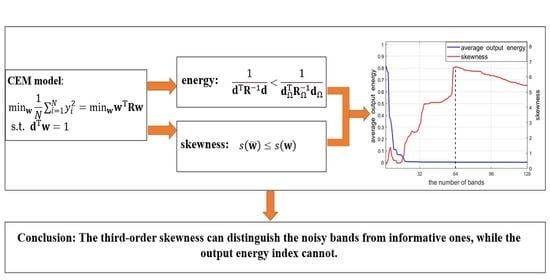
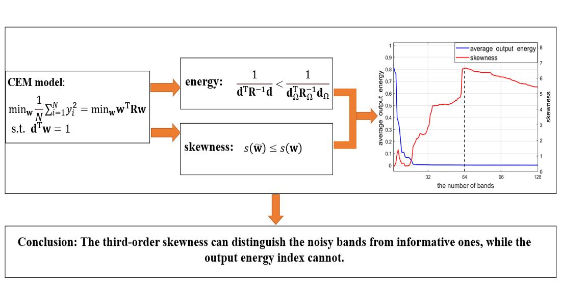
:Constrained energy minimization (CEM) has been proposed and widely researched in the field of hyperspectral target detection. Generally, it selects one of the target spectra as the representative and then keeps its output constant while minimizing the average filter output energy of the data. However, it has been proven that as the number of bands (L) increases, CEM will gradually lower the average filter output energy when keeping the representative’s output constant. Unavoidably, due to the inherent spatial and temporal variation of the spectra, this will lead to an unreasonable phenomenon, i.e., if L is particularly large, when adding more bands, CEM will suppress more and more pixels, even including the target pixels. This means that the optimal solution of CEM may not correspond to the target detection result that we desire. To deal with this, in this paper, we introduce the third-order statistic (skewness) of the CEM model, served as an auxiliary index to determine whether a band is beneficial to target detection or not. Theoretically, we prove that the skewness index can always exclude the noisy bands with Gaussian distribution. In addition, experiments on several widely used remote sensing data indicate that the index can also efficiently identify informative bands for a better target detection performance.
1. Introduction
Target detection is an important research area in the applications of remote sensing, such as climate change [1], camouflage target detection [2], agricultural production [3], land use [4], urban monitoring [5], ship detection [6], etc. Recently, with the development of technology, more and more hyperspectral data have become available and have been successfully applied for various applications. Accordingly, hyperspetral target detection has been obtaining more and more attention in the past few decades [7,8,9,10]. Theoretically, the spectral difference between target and background is the physical basis for hyperspectral target detection.
Currently, hyperspectral target detection methods can be divided into the following four categories: (1) algorithms based on spectral similarity index, which aim to calculate the spectral difference between target and background pixels. The most commonly used one is the spectral angle mapping [11]; (2) linear mixing model (LMM)-based algorithms, which assume that any mixed pixel can be regarded as a linear combination of endmembers [12]. The represented algorithms are orthogonal subspace projection [13,14], and non-negative matrix factorization [15,16]; (3) algorithms based on statistical index. Currently, the second-order statistic is widely applied and the classical methods include constrained energy minimization (CEM) [17], matched filter (MF) [18] and mixture-tuned matched filter [19]; (4) learning-based algorithms, such as multitask, metric learning, etc. [20,21,22,23]. In this paper, we will focus on the third class.
The most representative statistic-based target detection algorithm is CEM, which is originally derived from the linearly constrained adaptive beamforming in the field of signal processing. It keeps the output of the target as a constant (equal to 1), while suppressing the average filter output energy of the data to a minimum level. Many variants based on CEM have also been widely researched [24,25,26,27,28,29,30], such as multi-target CEM (MTCEM), hierarchical CEM (hCEM), clever eye (CE) algorithm, etc. MTCEM can be considered as a multi-target version of CEM, which constrains the outputs of multiple targets to be constant [24]. hCEM designs a hierarchical structure, including different layers of CEM to better suppress background pixels [25]. CE originally introduces the concept of the data origin into CEM and has been demonstrated to achieve the lowest output energy [26]. In addition, some researchers also investigated the impact of the number of bands on the target detection performance [31,32,33]. For example, by combining a dimensionality expansion (DE) strategy with CEM, a generalized CEM (GCEM) approach was proposed to mitigate the affect of the insufficient bands of the multispectral imagery. Geng et al. theoretically proved that more included bands will always lead to a better performance from the perspective of lower output energy.
However, a lower filter output energy is not equivalent to a better detection performance. In most cases, there is more than one target pixel in an image. The commonly adopted method in CEM is to select one of the target spectra as the representative, denoted . Due to the spatial and temporal variation, the same object has different spectra and the CEM model can only guarantee the output of constant, regardless of the other targets with similar spectra to , which implies that it may not be capable of detecting all targets.
Such a phenomenon is not obvious when the number of bands is not enough. On the condition that spectral difference between and the other target pixels is smaller than that between target and background pixels, CEM generally can extract all target pixels. Yet, when the number of bands becomes larger, the possibility that CEM extracts all the target pixels is smaller. In particular, if the number of bands is particularly high, when adding more linearly irrelevant bands, CEM will suppress more and more pixels even including the target pixels with similar spectra to . Undoubtedly, CEM will receive a poor performance from the perspective of detection accuracy, which is clearly not the result we desire. This indicates that the optimal solution of CEM may not correspond to the best target detection result.
Generally, a hyperspectral imagery consists of tens or hundreds of bands with a very high spectral resolution, and CEM always uses the full-band data for target detection. In view of the above analysis, how to identify informative bands or exclude meaningless bands for a given dataset is worth studying. In this paper, we introduce the third-order statistic (skewness) into the CEM model, which is designed as an auxiliary index for the second-order statistic (the average output energy criterion) adopted in CEM. By investigating the third-order statistical characteristic of the CEM output, the index is expected to help to identify informative bands to further improve the accuracy of target detection.
The rest of this paper is organized as follows. In Section 2, we briefly review the classical CEM algorithm and discuss the paradox and the applicable conditions of CEM. In Section 3, we introduce the auxiliary skewness index, and theoretically prove that once the noisy band with the Gaussian distribution is added, the skewness will always decrease, compared to that of the original data. Some experimental results using simulation and remote sensing data are given in Section 4, and the conclusions are drawn in Section 5.
2. Preliminaries
In this section, we first briefly review the CEM algorithm and analyze the paradox in it based on the presented theorem. In the end, we discuss the application conditions of CEM with a simple example for illustration.
2.1. CEM
Denote the data as , where L is the number of bands, and N is the number of pixels. is the target vector. CEM aims to find a direction to minimize the average output energy while keeping the output of constant, which can be expressed as follows:
where is a scalar, is the auto-correlation matrix of . By using the Lagrangian method, the solution of (1) can be obtained
where is a constant for simplicity. Note that . See (A1)∼(A3) in the Appendix A for details. Then, the objective function in (1) can be calculated by
It can be seen that the constant c is equal to the average output energy of CEM for .
2.2. Paradox in CEM
Many variants have been developed based on CEM. In [32], by incorporating the DE strategy into CEM, GCEM was presented, which aims to produce new additional bands to provide useful information for target detection and make CEM more effective. Later, Geng et al. theoretically prove that adding arbitrary bands linearly irrelevant to the original data would be helpful to achieve a lower average output energy for CEM. Given a data set , and suppose that is an arbitrary subset of the band index set. , are the corresponding auto-correlation matrix and target vector, respectively. The following theorem holds.
Theorem 1.
The output energy from full bands is always less than that from the partial bands, i.e.,
The detailed proof can refer to [33]. Theorem 1 indicates that when more bands are included, the performance of target detection will always be improved from the perspective of the average output energy.
It seems that this conclusion is theoretically safe, but it will lead to a paradox in practice. We assume that one noisy band is added into . On the one hand, based on Theorem 1, the noisy band irrelevant to will improve the performance of CEM from the perspective of a lower average output energy. On the other hand, adding a noisy band actually does not provide any useful information to better distinguish the target of interest from the background. This indicates that it should not bring any benefit to the target detection result. Therefore, here emerges a paradox. Even though adding noisy bands can theoretically lower the output energy, they will be treated as bad ones in practice. Therefore, if blindly focusing on the descent of the energy, we will fail to distinguish these noisy bands from the informative ones.
Motivated by these observations, we raise several interesting questions:
(1) What is the intrinsic reason for such a paradox between theoretical analysis and practical applications?
(2) How to reconcile this contradiction and to reject these useless bands (e.g., noisy bands)?
We aim to address the above questions and the details are discussed in the following.
2.3. Remarks on CEM
As can be seen from (1), CEM is only suitable for single target detection, and it also assumes that there is only one target vector (i.e., ) for this class of target (denoted ). However, in real applications, due to the spatial and temporal variation, the same object has different spectra, and there may be more than one target pixel for in an image. Suppose that the number of different target pixels is M, and their corresponding spectral singnatures are denoted . When using CEM, we usually select one of the targets (e.g., ) as the representative one. Concerning the CEM model, we have the following several remarks:
Remark 1
(The theoretical premise for CEM). Concerning the case that there are M pixels for one target, CEM implicitly uses the premise that the target spectrum does not change, i.e.,
Unfortunately, for most of the real remote sensing data, due to the spatial and temporal variation, the spectra of M targets cannot be the same, and the premise (5) does not hold in many practical cases. Therefore, it is necessary to further discuss the application conditions of CEM in practice, which are remarked as follows:
Remark 2
(The practical application conditions of CEM). CEM would obtain a satisfactory result in practice if one of the following conditions are met:
- the spectral variability of the targets is relatively small;
- the spectral variability of the target is smaller than that of the target and the background.
Fortunately, in real applications, many data meet the above conditions. Therefore, CEM is widely applied and can obtain a satisfactory result in most cases. Instead, the hidden premise (5) is universally ignored and rarely discussed.
In addition, another fact that should be pointed out is that the number of bands (L) is usually far less than the number of pixels (N) in most applications. In this case, even the spectra of targets () are different to each other to some extent, and CEM can extract all target pixels in general. In contrast, when L is particularly large, due to the spatial and temporal variation of the spectra, a phenomenon which we termed as “suppressing the target pixels with similar spectra to the representative)” begins to emerge, which is remarked as follows:
Remark 3
(The “suppressing the target pixels with similar spectra” phenomenon). Theoretically, by Theorem 1, including more bands will lead to a better performance. Practically, if L is particularly large, when adding more linearly irrelevant bands, CEM will suppress more and more pixels, even including the targets with similar spectra to (target pixels ).
It can be explained by considering an extreme case, which is stated as the following lemma:
Lemma 1.
Given a data set , there are M linearly irrelevant samples for the targets of interest (denoted ). Without losing of generality, we select a target as used in CEM. When , and the columns of the data are assumed to be linearly independent, only the CEM output on is equal to 1, while the outputs on the left pixels (including ) are always equal to 0.
The detailed proof is presented in the Appendix A. In practice, since , all target pixels can still be effectively detected by CEM in most cases. However, when more linearly irrelevant bands are added which makes L comparable with N, even though the average output energy will always be lowered, the detection performance may also be degraded. As implied by Lemma 1, when , only the target selected as the representative one (i.e., ) can be detected (highlighted), while all the other targets (i.e., ) are suppressed, which clearly is not the result that we expect. This means that the optimal solution of CEM may not correspond to the target detection result that we desire.
2.4. Motivation
In this part, we use a simple example to intuitively demonstrate the claim that more bands may not always bring about the improvement of target detection. Simulation data are generated as follows:
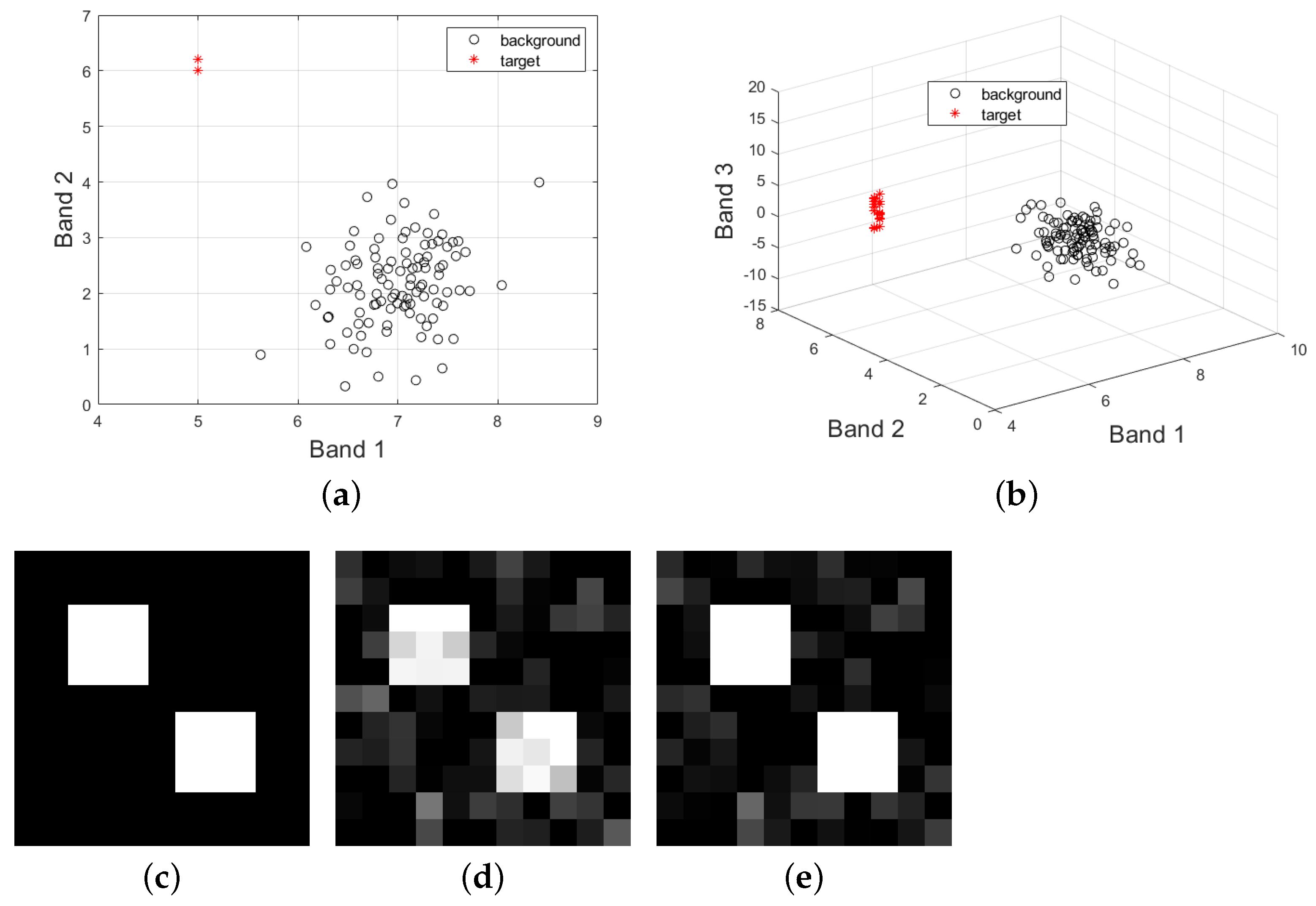
(1): a background image with a size of is firstly generated. It follows an 2-dimensional normal distribution, whose mean vector is set to , and the covariance matrix of the data is respectively.
(2): two target images with the same size of are added into the background data. The corresponding groundtruth image is shown in Figure 1c. We set all the target vectors of the upper left region as , and those of the lower right region as . The distribution of the simulation image in 2-dimensional spectral space is shown in Figure 1a, where the background pixels are marked in black circles and the target ones are marked in red asterisks.
(3) Then, a noisy band, whose mean and variance are all equal to 2, is added into the above data with two bands. Correspondingly, the distribution of the simulation image in 3-dimensional spectral space is shown in Figure 1b.
As can be seen, the values of , are a little different, and they are away from the background points, which satisfies the condition mentioned in Remark 2 of Section 2.3. Therefore, it is expected that both of them will be identified as the target of interest when using CEM. Next, we consider the performance of CEM in two different cases:
- using full-band data ();
- using Band 1, 2 ().
We select the first pixel of the target image at the upper left corner as .
Correspondingly, the CEM results using different Ls are shown in Figure 1d,e, respectively. It can be observed that when using the data with full bands, only the representative one is highlighted, while the other target pixels are suppressed to some extent. In contrast, when only using Band 1 and 2, both and are highlighted, whose result is instead superior to that of .
In addition, we calculate the average output energy of CEM, and the results are tabluated in the first row of Table 1. Consistent with the conclusion in Theorem 1, the average output energy for the data with 3 bands is smaller than that with 2 bands. However, the results comparison in Figure 1d,e indicates that the data with more bands does not lead to a better performance. As implied by Lemma 1, when more bands are added, the target pixels with similar spectra to may be suppressed, which instead degrade the performance. Such an example indicates that a lower average output energy is not equivalent to a better target detection.
As mentioned above, Band 3 is a noisy one, which cannot increase the separability between the target and the background. In this case, how to identify informative bands (Band 1 and 2 in this example) is an interesting problem that needs to be solved. Clearly, the energy criterion cannot exclude Band 3, because either an informative band or a meaningless one will indistinguishably lower the average output energy. To deal with this issue, similar to calculating the average output energy of the CEM output, we try calculating its third-order statistic, whose results are tabulated in the second row of Table 1. As can be seen, when , the absolute value of the skewness is smaller, compared to that of the data of . This motivates us to introduce the skewness index into CEM, as an auxiliary index to identify whether a newly-added band is beneficial to the target detection. Once the skewness metric decreases when a new band is added, we treat it as a useless band and exclude it from the data. In contrast, if the skewness metric increases, it will be considered as an informative band to be included.
Motivated by this, we design an auxiliary index for CEM, and further exploit some theoretical gaurantee for such a new index. The details are as follows.
3. Third-Order Statistic–Skewness
In this section, we first introduce the definition of the skewness index for the CEM model. Then, we mainly focus on a special case, and investigate how the skewness will change when noisy bands with Gaussian distribution are added. Finally, we discuss how to utilize the skewness index in real applications.
3.1. The Skewness Index for CEM
Given an arbitrary random variable , its skewness is defined as
where u is the mean value of , r is the standard deviation of . In addition, we consider the absolute value of skewness by default.
More specifically, for the case of CEM, after obtaining the CEM detector given data , we can compute the absolute value of the skewness metric of projected along , which is expressed as
where , is the third-order and second-order cumulant of .
3.2. Analysis for Cases with Added Noisy Bands with Gaussian Distribution
It should be noted that the analysis in Table 1 is based on a numerical comparison. In the following, we will focus on analyzing how the skewness metric will change when the noisy bands with Gaussian distribution are added. Without losing generality, we will only consider the case of adding one noisy band. More noisy bands cases can be analyzed in a similar way.
We consider a new data denoted
which is composed of and 1 newly-added noisy band . We assume that the noisy band follows the Gaussian distribution with zero mean (), and the variance of is , where r is the standard deviation of ( ). In addition, we assume that the noisy band is independent to .
It is easily checked that the auto-correlation matrix (denoted ) of can be expressed as
where is an column vector with all elements equal to 0. Next, we consider the target detection result of CEM on , and the corresponding target of interest to be detected is denoted , where d is a scalar. Then, the CEM detector of (denoted ) is calculated by
where is the average output energy of CEM for ( Similar to the analysis for c based on (A1)–(A3) in the Appendix A, it also holds that ). In addition, it holds
Then, the filter vector for is given by
It can be seen from (11) that , indicating the average output energy for , is always no larger than that for , which is consistent with the conclusion in Theorem 1. An interesting question is what the skewness of the CEM output of will change, compared to that of . We will focus on this issue and the following theorem is presented:
Theorem 2.
Given a data set as in (8), composed of and 1 noisy band that follows the Gaussian distribution. We assume that the noisy band is independent to . It holds that the skewness of the CEM output of is always no larger than that of , which can be expressed as
The detailed proof is presented in the Appendix A. The key point of the above proof lies in that the noisy band is assumed to follow the Gaussian distribution, and its high-order statistics will always equal zero. By comparing the Theorems 1 and 2, we can also see the differences between the second-order statistic (the average output energy used in CEM) and the third-order skewness. The average output energy will always decrease when either an informative band or a noisy one is added. Theorem 2 indicates that when a noisy band that satisfies Gaussian distribution is added into a data set, the corresponding skewness of the CEM output will always be no larger than that of the original one. Such a conclusion provides a theoretical guarantee for the utility of skewness in CEM, which can efficiently exclude the noisy bands that follow the Gaussian distribution by monitoring the skewness change.
We can go further to consider the skewness utility in real applications. Although the band for real data sets does not always follow the Gaussian distribution, we can make the final decision based on numerical skewness comparison, motivated by the simple example tabulated in Table 1 and the conclusion in Theorem 2. Given a data set, when the k-th band is removed, if the skewness of the CEM output of the new data increases or keeps unchanged compared to that of the original one, we treat the k-th band as a useless one and exclude it out of the data. In contrast, the band will be reserved as an informative band to be included.
4. Experimental Results
In this section, both simulation and real remote sensing experiments are conducted to evaluate the effectiveness of the skewness index. The simulation part mainly considers the cases with added noisy bands with the Gaussian distribution, and compare the average output energy and skewness change. For the real data part, movitated by the simple example in Figure 1 and the theoretical analysis in Theorem 2, we mainly focus on investigating the impact of different Ls on the target detection performance, and whether the skewness index can serve as a tool to identify informative bands for a better detection result.
To quantitatively evaluate the performance of target detection, the widely used metrics, including receiver operating characteristic (ROC) curve, area under the ROC curve (AUC), overall accuracy (OA), F-score, and Cohen’s kappa coefficient are used. For the ROC curve and the corresponding AUC value, they are directly calculated based on the CEM output. The other three metrics are computed based on the binary classification of the output, which is obtained by using the threshold method [34]. The optimal threshold is determined from the ROC curve by the Younden index. Then, based on the classification result, the confusion matrix is defined in Table 2.
Then, the OA index is computed by
The F-score metric (denoted ) is defined as
where
and is the weight of precision in harmonic mean and is set to in our experiments. Denote
The Kappa coefficient (denoted ) can be calculated by
For the four quantitative metrics, a higher value indicates a better performance of target detection. It should be noted here that, since the targets selected in our experiments for the real remote sensing data are “small” targets, whose size is much smaller than that of background. For a fair comparison, the background pixels are randomly selected, whose numbers are equal to the number of reference target pixels [35], and the average OA, F-score, and kappa coefficient of 20 runs are computed in our experiments.
All the algorithms are implemented in MATLAB on a laptop of 12 GB RAM, Inter(R) Core (TM) i7-10510U CPU, @ GHZ.
4.1. Simulation Experiments: Identify the Noisy Bands with Gaussian Distribution
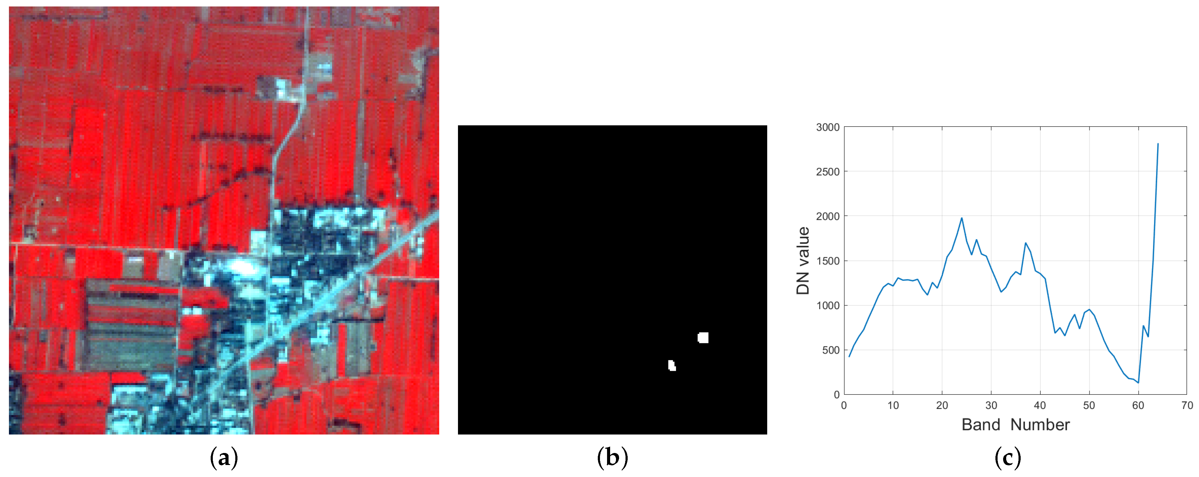
In this part, we mainly analyze how the skewness metric will change when the noisy bands with Gaussian distribution are added. Here, a hyperspectral image is used to conduct the experiment. It was collected by the Operational Modular Imaging Spectrometer-II, which is a hyperspectral imaging system developed by Shanghai Institute of Technical Physics, Chinese Academy of Sciences, and was acquired in the city of Xi’an, China in 2003 (named Xi’an data). It contains 64 bands from 460 nm to 10,250 nm in 3.6-m spatial resolution and each band is with pixels. The false color composite image is shown in Figure 2a.
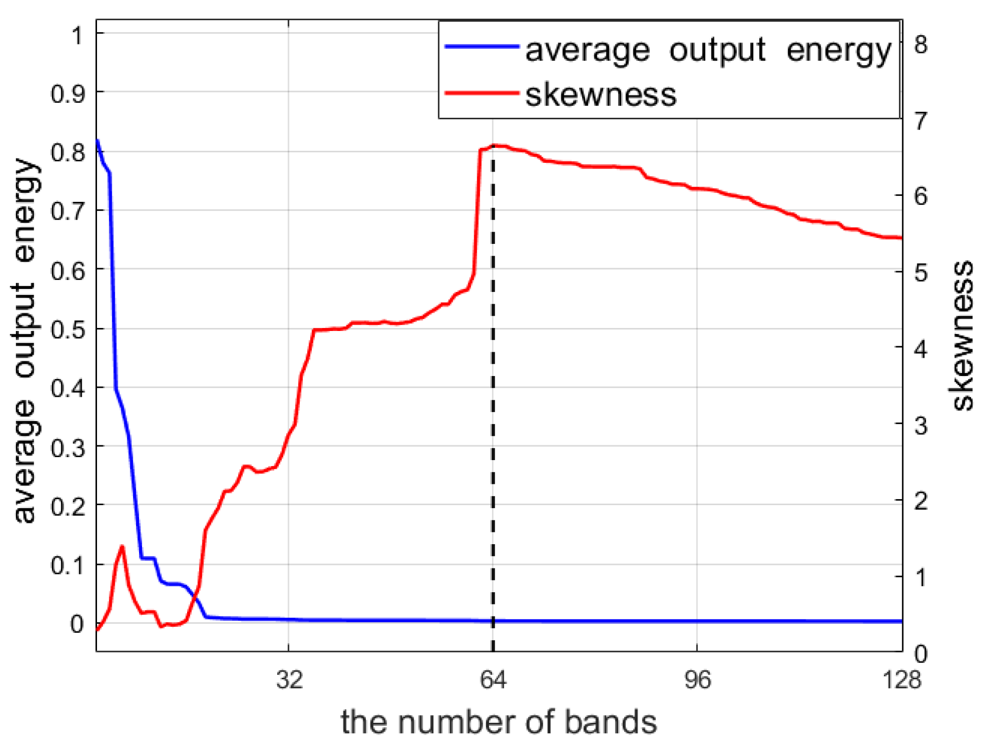
As can be seen, the average output energy of the CEM output always decreases, whether the band of the data or the noisy band with Gaussian distribution is added. This is consistent with the conclusion in Theorem 1 and implies that the energy criterion cannot distinguish the informative bands from the noisy ones. As a contrast, the skewness of the CEM output gradually declines once the noisy bands that obey Gaussian-distribution are added, which has a clear watershed (the black vertical line in Figure 3). This is also consistent with our presented Theorem 2. The above curves comparison concerning the average output energy and the skewness index further confirms our discussion in Section 2.3 and the theoretical analysis in Section 3.2. To conclude, the simulation result indicates that:
- the second-order statistic used in CEM (i.e., the average output energy) is unable to distinguish the noisy bands from informative ones;
- by comparison, the introduced third-order skewness index can actually serve as an efficient tool in identifying the noisy bands with Gaussian distribution.
We manually add some noisy bands that follow Gaussian distribution to the original data, and record the change of the energy and skewness. More specifically, the experiment is conducted based on the following steps (Algorithm 1):
| Algorithm 1 The process for plotting the energy and skewness curve as a function of L |
| (1). we select the first two bands as the initial data, where and the corresponding data are denoted . Then, we can calculate the CEM output and its average output energy and skewness. |
| (2). Sequentially, we add the Band into one by one, and record the corresponding average output energy and skewness values. |
| (3). When all bands are included (), we keep on adding simulated noisy bands with Gaussian distribution one by one into the full-band data, and also calculate the average output energy and skewness metrics. The noisy band that follows Gaussian distribution is randomly generated by the function in the Matlab software. Here, the maximum number of the noisy bands is set to 64. |
| (4). We plot the average output energy and skewness curves as a function of L, ranging from 2 and 128. The corresponding results are plotted in Figure 3. |
4.2. Real Experiment 1: Evaluate Each Band of the Original Data
4.2.1. Xi’an Data
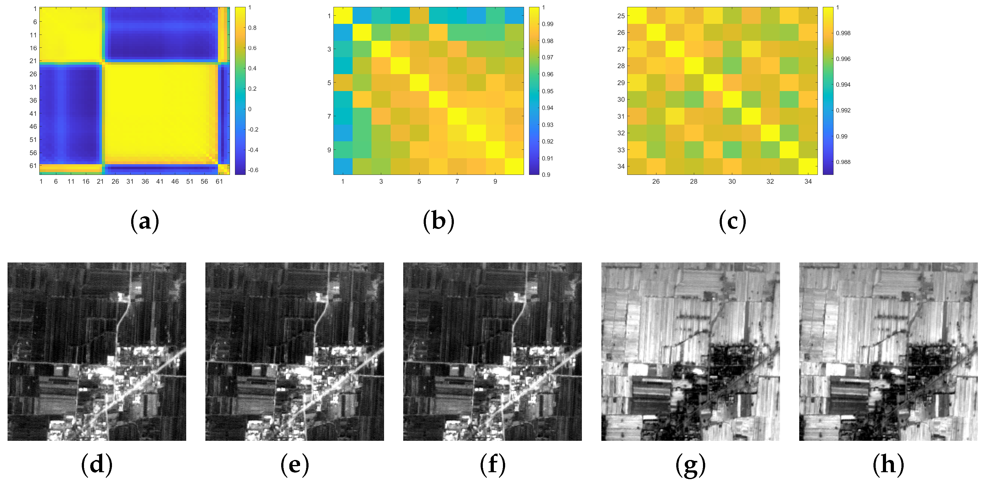
We start this part by reobserving Figure 3. Another interesting phenomenon is that when some bands of the data are added, the skewness values of the corresponding CEM output also decrease, such as Band 6–8, Band 26–27, etc. We first calculate the correlation coefficient between two random spectral bands, and the corresponding correlation coefficient image with a size of is shown in Figure 4a. The zoom image of Figure 4a for Band 1–10 and Band 25–34 is also displayed in Figure 4b,c. Meanwhile, the images of these bands are shown in Figure 4d,h. The corresponding correlation coefficient between Band i and j (denoted ) for these bands is attached for clearness. It can be found that these bands are with a high correlation coefficients and Band 6–8 or Band 26–27 have no clear distinction visually. Concerning the target detection task, these highly correlated bands cause informative redundancy and it may be uncessary to include all of these bands, since they may not provide extra useful information to better distinguish the target of interest from the background. Thus, inspired by the Theorem 2, the introduced skewness index seemingly can also serve as a tool to identify these bands that have high correlations and have less contribution or benefit to the target detection result.
We still use the Xi’an data to verify our conjecture. In this area, there are two small man-made targets and the manually determined groundtruth map based on the field survey is shown in Figure 2b. The selected spectrum of the target of interest is plotted in Figure 2c. Then, we consider the target detection result by introducing the skewness index. More specifically, the experiment is conducted based on the following steps (Algorithm 2):
| Algorithm 2 Band selection process using the skewness index |
| (1) Initial input: we select the data with L bands and N pixels as the initial input, denoted . Then, we compute the CEM detector of (denoted ) and the skewness according to (7). Set , and k = L. |
| (2) Band deletion: assume the k-th band of is removed. Set . Denote the new data . Similarly, the CEM detector of (denoted ) and the corresponding skewness can be calculated. |
| (3) Skewness comparison: if , we treat k-th band as a less-contributive band and delete it out of . Otherwise, the k-th band should be reserved. Then, update and k = . |
| (4) Repeated process: repeat step (2)–(3), and compare the skewness value before and after the k-th band is removed, to determine whether this band will be deleted or not. |
| (5). Stop condition: the process is terminated until there are two left bands, and eventually we obtain new data with smaller L. |
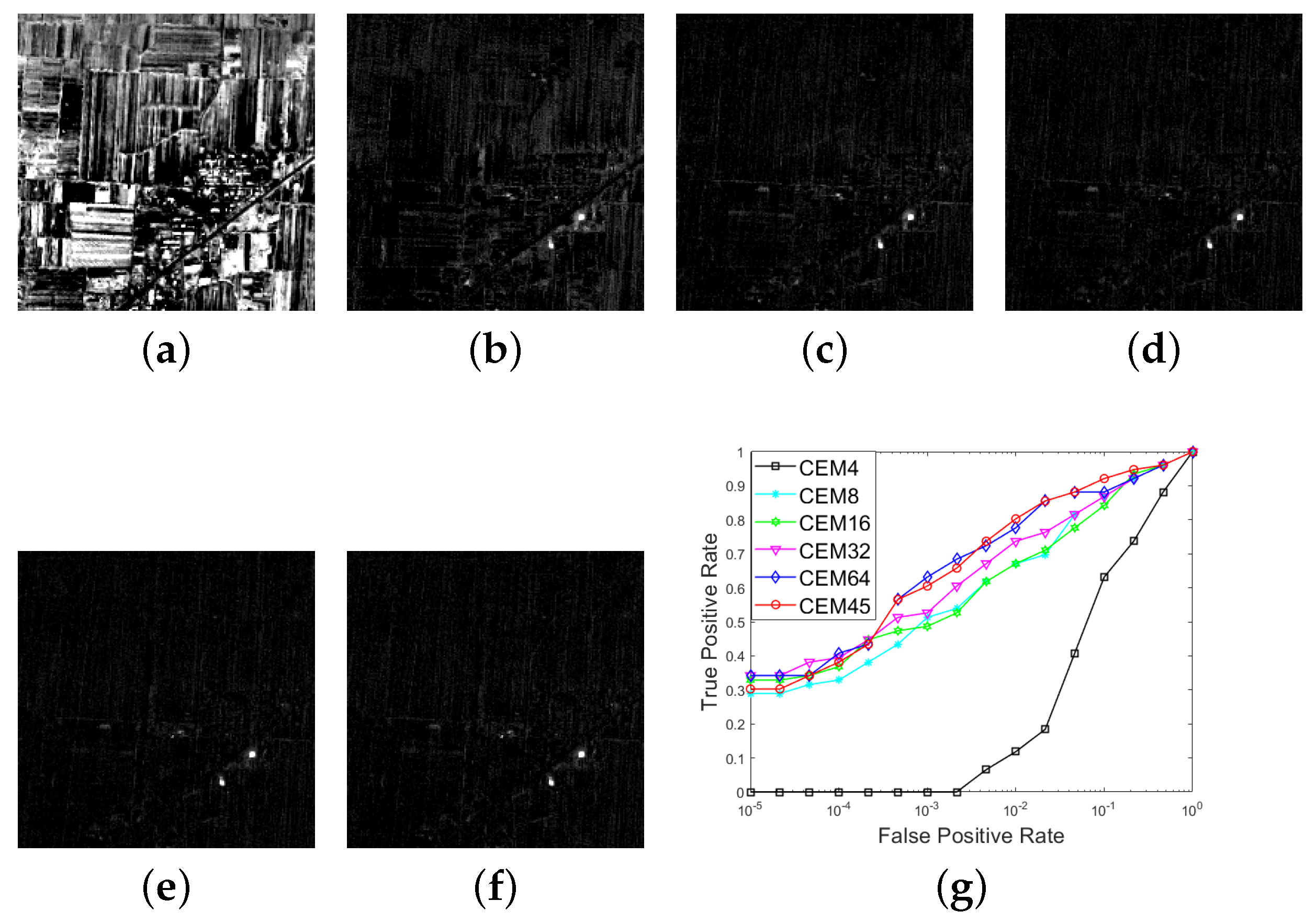
Note that the above steps can be viewed as a band selection process, where the skewness value is compared between the data with k and 1 (k = L, 1, …, 3). In this experiment for the Xi’an data, the total number of these deleted bands suggested by the skewness metric is 19. We then use the left 45 bands () for target detection, whose result (denoted CEM45) is shown in Figure 5f. Next, we also compare the performance of target detection using different Ls. In this experiment, we set . Data with 32 bands were generated via down-sampling by averaging the data every 2 bands. The other data with 16, 8, 16, or 4 bands is obtained in a similar way. Correspondingly, the target detection results are denoted CEM4, CEM8, CEM16, CEM32, and CEM64, respectively, as shown in Figure 5a,e.
By comparison, it can be seen that when the data with are used, we cannot detect the targets of interest at all. When 8 bands are used, though the targets of interest are highlighted, there are some false alarms that are highlighted. It is a little difficult for the other results to visually determine which one is better. In addition, the ROC curves comparison for these results are plotted in Figure 5g. Similarly, the curves are very close, and we cannot still evaluate their performance. Therefore, for a quantitative comparison, we turn to calculating the four metrics mentioned before, whose results are tabulated in Table 3. As can be seen, the metrics using the original data have been very high, which is also consistent with our presented Remark 2, and indicates that when the spectral variability of the targets is relatively small, CEM can obtain a satisfactory result in most cases. Furthermore, the AUC value of CEM45 where the skewness is introduced is still higher than that of the original data (CEM64), which can demonstrate the superiority of introducing the skewness index. This confirms our conjecture analyzed in the beginning of this part. By utilizing the skewness index and comparing the skewness value before and after one band is deleted, we can identify the highly correlated bands in a data set and exclude some of them out of the data. The quantitative comparison results indicate that the result using these bands combinations selected by the skewness index provides a better performance for target detection. The quantitative comparison results also demonstrate that the result of CEM45 is better than that of the other cases.
4.2.2. YC Lake Data
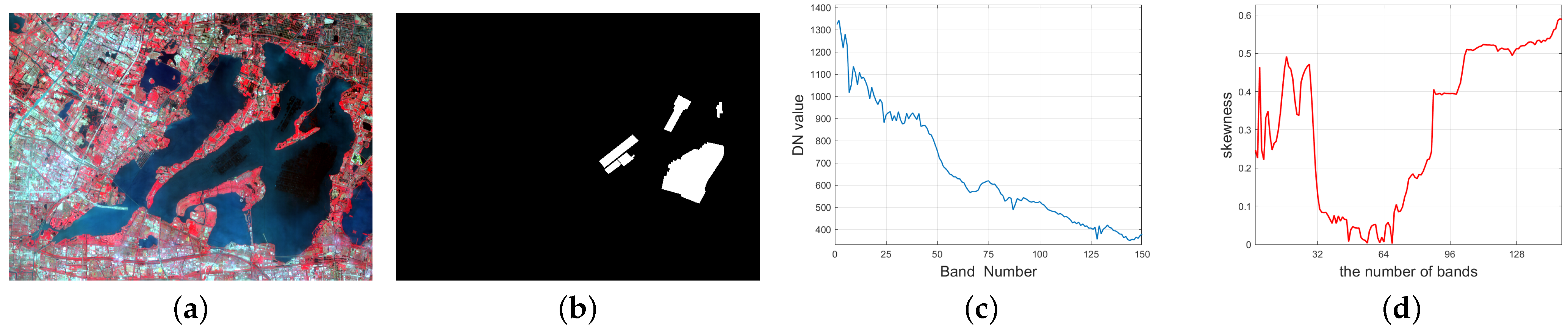
In this part, another hyperspectral data set is used, which was acquired by Gaofen-5 (GF5) satellite at Yangcheng lake of Jiangsu Province, China. And the data is termed the YC Lake data set. It contains 150 bands with wavelengths ranging from 390.32 nm to 1029.18 nm in 30-m spatial resolution, and each band has pixels. The corresponding false color image is shown in Figure 6a. With the development of fishery and aquaculture in lakes, pen culture is mainly conducted, which makes it the most significant form of aquaculture in shallow lakes in China. In this experiment, we will select the pen culture as the target to be detected, and the groundtruth image for the pen culture is shown in Figure 6b. The selected spectrum of the target is shown in Figure 6c.
Similar to the processing steps (1)∼(2) in Section 4.1 of Section 4, we can plot the skewness curve as a function of L, ranging from 2 to 150, whose result is shown in Figure 6d. Consistent with the result for the Xi’an data, the skewness value also decreases when some bands are added. We also calculate the correlation coefficient between two sepctral bands, and the corresponding correlation coefficient image with a size of is shown in Figure 7a. We display some gray images of the bands deleted by the skewness criterion (Band 19-21, 113-115), as shown in Figure 7. For clearness, two zoom correlation coefficient images for Band 15–24 and Band 111–120 are also displayed in Figure 7b,c. The corresponding correlation coefficient between Band i and j (denoted ) for these bands, also attached. It can be seen that Band 19–21 or Band 113–115 are visually similar and highly correlated, respectively. Moreover, the introduced skewness metric can automatically suggest excluding these bands.
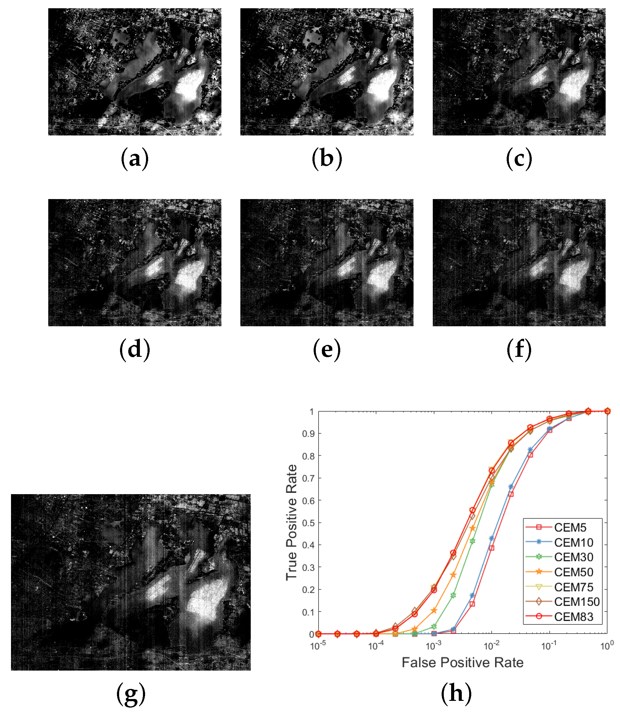
We can perform the band selection process based on the skewness comparison which is similar to step (1)–(4) in Section 4.2.1. The initial input data are with . The number of the deleted bands is 67 here. Then, we use the left 83 bands () for target detection, and the result is denoted CEM83. Meanwhile, the target detection performance using the data with different Ls is also compared, which are set to here. Correspondingly, the CEM results for these cases are shown in Figure 8a–g. When only 5 bands are used, though the area of the pen culture is approximately detected, there are also many false alarms, and the quantitative metrics are also inferior to the other cases, as shown in Table 4. The performance of CEM75 is also superior to that of CEM150, which also confirms the analysis that more participated bands may not bring a better performance. With band selection based on the skewness comparison, the performance of CEM83 is further improved compared to that of CEM75. In addition, the quantitative metrics of CEM83 are higher than that of other cases, which have an overall better performance.
For the hyperspectral imagery that consists of tens or hundreds of bands, there exists strong intraband correlations. From the perspective of target detection, these highly correlated bands usually do not bring extra information for distinguishing the targets from the background. Combining the comparison results for the two data set, we conclude that the introduced skewness index can actually serve as an efficient tool in identifying these highly-correlated bands of the data, and we can use these left informative bands to further improve the performance of target detection.
4.3. Real Experiment 2: Evaluate the Generative Bands by GCEM
In this part, we will make some comments about the DE strategy used in the GCEM algorithm. Since the insufficient dimension of the multispectral imagery, GCEM has been proposed, which aims to produce additional bands to provide useful information and to detect the targets more effectively. In [32], there are several DE approaches that can be used, including auto-correlation, cross-correlation, and nonlinear correlations. The authors suggested two nonlinear strategies, including the use of the square-root and logarithm function. More specifically, denote L bands of as , the generative bands are obtained using the following methods (Algorithm 3):
| Algorithm 3 Four DE strategies used in GCEM [32] |
| (1): L auto-correlated spectral bands: . |
| (2): cross-correlated spectral bands: . |
| (3): L spectral bands stretched out by the square-root: . |
| (4): L spectral bands stretched out by the logarithmic function: . |
Eventually, for the data with L bands, by using the DE strategy, we can obtain the newly generative data with bands.
Here, the data set used in this experiment is the well known Indian Pines data, which was gathered by the Airborne Visible/Infrared Imaging Spectrometer (AVIRIS) sensor over a mixed forest/agricultural site from Northwestern Indiana, USA, on 12 June 1992. It contains 220 bands with the wavelength ranging from 0.4 μm to 2.5 μm, and each band has a size of with an 20 m spatial resolution per pixel. By manually removing 20 water vapor absorption bands (Bands 104–108, 150–163 and 220), there are 200 left bands. The false color image is shown in Figure 9a.
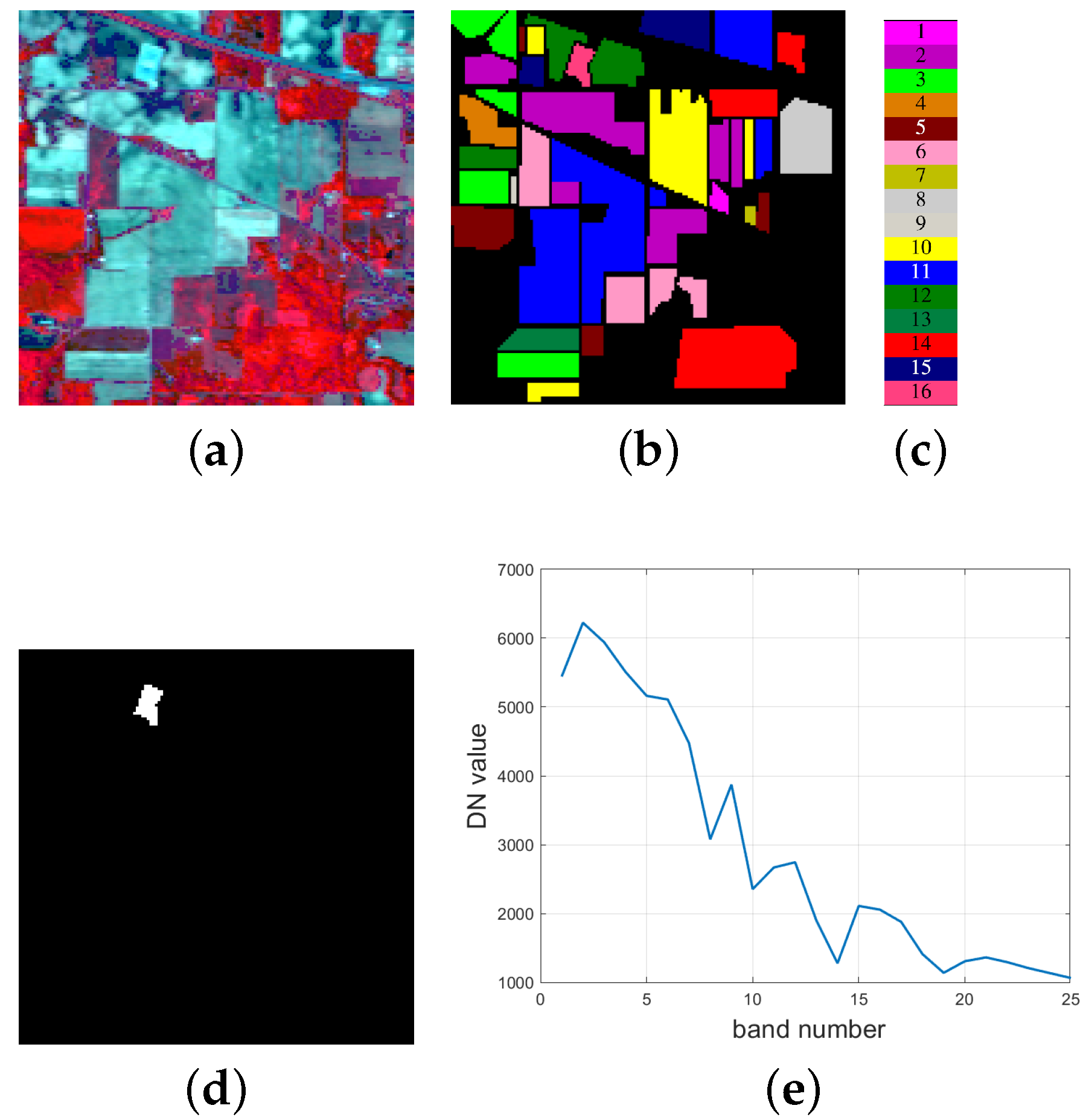
This data set contains 16 classes of land cover types, and the classes name and the number of samples for each class are tabulated in Table 5. It can be seen that the main land cover type of this data is vegetation. Specifically, it contains two-thirds agriculture (such as corn-like classes (classes 2–4), soybean-like classes (classes 10–12)), and one-third forest (such as grass-like classes (classes 5–7) or other natural perennial vegetation (such as alfalfa (class 1)). Except for the vegetation, the 16th class corresponds to the stone-steel-towers land cover type. The groundtruth data for the 16 classes is displayed in Figure 9b. In this experiment, we select the 16th class as the target of interest. This is based on the following considerations: (1): For class 16, its spectra are obviously different from those of the other vegetation-related land cover types, which satisfies the condition that the spectral variability of the target is smaller than that of the target and the background, as analyzed in Remark 2 in Section 2.3. (2): There are only 10,249 pixels that are labeled, while the left 10,776 pixels are not well classified, which may belong to one of these vegetation land cover types. Therefore, it is unreasonable to select one of the other classes as the target of interest, since their groundtruth is not accurate. The groundtruth image for the target is shown in Figure 9d. Firstly, we use the band average strategy as mentioned in Section 4.2.1 to obtain a multipsectral image with a lower number of bands. And here, L of the multipsectral data is set to 25. Correspondingly, the spectrum of the target for the data with 25 bands is plotted in Figure 9e.
Using the DE strategy in (1)–(4), we can obtain a series of generative bands, and obtain new data with eventually, whose CEM result is denoted CEM400. It can also be inferred that not all of the generative bands by the DE strategy are beneficial to the target detection. By comparing the skewness change similar to the above experiments, the skewness index can also be designed as a tool to evaluate whether a generative band is an informative or useless one, and to exclude some useless bands out of the data.
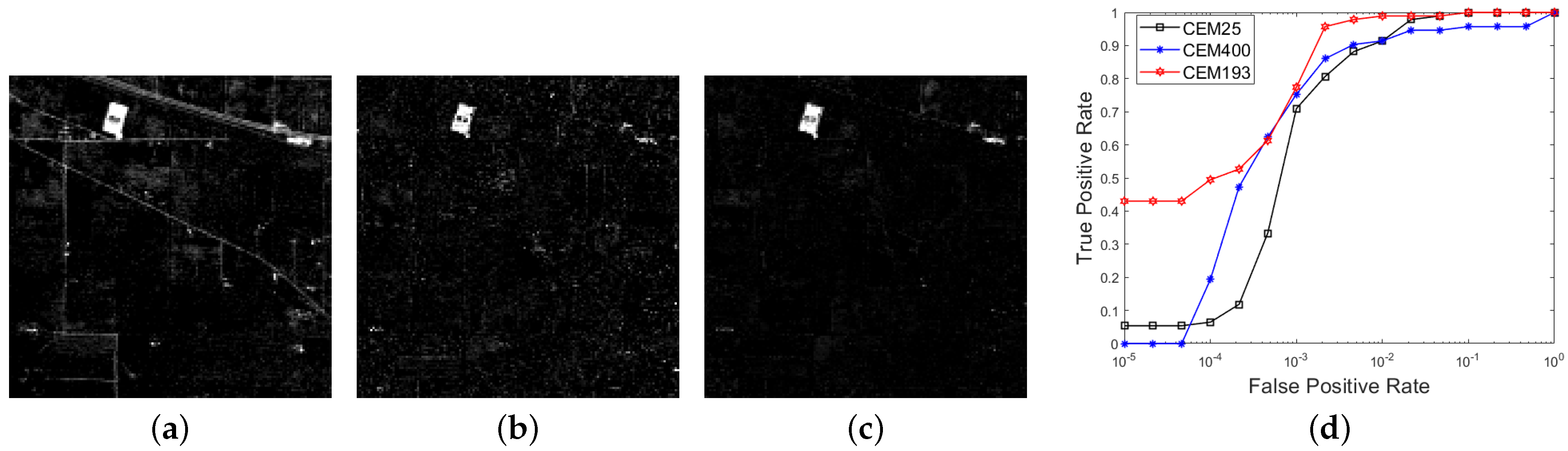
Similar to step (1)–(4) in Section 4.2.1, we input the data generated by GCEM (), and perform the band selection process. Eventually, data with are returned, and the correspondingly CEM result is denoted as CEM193, whose result is shown in Figure 10c. As a comparison, the results for CEM25 (the multispectral data with 25 bands) and CEM400 (the data generated by GCEM) are also shown in Figure 10a,b, respectively. The ROC curves for these results are plotted in Figure 10d. In addition, the quantitative comparison for the four metrics is tabulated in Table 6. It can be seen that: (1) The comparison of the GCEM result (CEM400) and CEM25 further confirms our conclusion presented before—more bands may not lead to a better performance. Thus, though the DE strategy used in the GCEM algorithm is efficient to increase the dimensionality of bands, it may not always provide a positive improvement to target detection, due to the inherent spatial and temporal variation of the spectra; (2) the result of CEM193 is superior to that of CEM25 and CEM400, which also verifies our viewpoint and demonstrates that the skewness index can serve as an efficient tool to evaluate whether the generative band is beneficial and to further improve the performance of target detection.
By combining the experimental results in both simulation and real data parts, we conclude several advantages of introducing the skewness index into CEM as follows:
- As demonstrated by the theoretical analysis in Theorem 2 and the simulation experiment, the absolute value of the skewness index for the CEM output will decrease when the noisy bands with Gaussian distribution are added, compared to that of the original data. Therefore, in theory, the introduced skewness index can always identify these noisy bands and exclude them out of the data.
- In addition, the skewness index can also serve as a tool to score the contribution of the band of the data to the target detection, and exclude these highly-correlated bands to further improve the performance.
- When the DE strategy is used to generate new bands, the skewness index can also serve as an auxiliary tool to evaluate whether the generative band is a contributive one or not, and intellectually select these informative bands for better performance.
4.4. Computational Complexity and Future Works
In this part, the computational complexity of the proposed method is analyzed. For the data with L bands and N pixels, when we delete a band and update the corresponding skewness value, we need to recalculate the auto-correlation matrix, denoted , of the data with bands, denoted , and its inverse matrix denoted , whose computational complexity is given by and , respectively. The complexity of calculating the CEM output and the skewness value of the output is and . Then, we go on deleting another one band from and repeat the above calculations. Therefore, the total complexity of the band selection process is given by .
However, after some literature research, we found that the calculation of (k = L, 1, …, 3) can be obtained by the following recursive formula: , where , and is the auto-correlation matrix of the data with k bands (, , …, 3), is its inverse matrix, is a matrix with a size of , composed by the first -th row and column of , is an vector with a size of , and a is a scalar. More details about the derivations can refer to the original reference [36]. In this way, we only need to calculate and , and can be recursively obtained by . Thus, the complexity of computing can be reduced from to . Meanwhile, the calculation of is also avoided by using such a formula. Therefore, the total complexity can be further reduced to . However, since N is usually large given an image, it is still time-consuming in real applications. In the future, how to further reduce the complexity and to accelerate the skewness calculation process is worth studying.
5. Conclusions
CEM is one of the most widely applied algorithms in the field of remote sensing target detection. However, due to the spatial and temporal variation of the spectra, CEM can only guarantee the selected representative target to be detected, while the other target pixels with similar spectra to it may be suppressed. In particularly, as the number of bands increases, such a phenomenon is becoming more and more obvious. In this paper, to deal with this issue, we introduce the third-order statistic—skewness into the CEM model, which is designed to serve as an auxiliary index to identify whether a band is contributive to target detection or not. We have theoretically proven that the skewness index is always capable of excluding the noisy bands with the Gaussian distribution, which is also confirmed by the simulation experiments. In addition, experiments on several real hyperspectral data set also show that it can be utilized in a band selection process, which can (1) discard the highly correlated bands of the data; (2) evaluate whether the generative bands by GCEM are informative or not. The comparison results demonstrate that introducing the skewness index into CEM can identify informative bands to further improve the performance of target detection.
On the other hand, a band selection process using the skewness index also suffers from a higher computational complexity compared to the original CEM method. We have adopted a recursive update formula at the end of Section 4 to accelerate the calculation. However, more efforts should be made to make it suitable for large-scale data. This will be researched in the next stage.
Author Contributions
Experiment and writing: L.W.; methodology and data collection: L.J. and X.G. All authors have read and agreed to the published version of the manuscript.
Funding
This work was supported by the National Key Research and Development Program of China under Grant 2016YFA0600103.
Institutional Review Board Statement
Not applicable.
Informed Consent Statement
Not applicable.
Data Availability Statement
Not applicable.
Conflicts of Interest
The authors declare no conflict of interest.
Appendix A
In this part, we give detailed proofs for the lemma and theorem presented in the paper.
Lemma A1.
Given a data set , there are M linearly irrelevant samples for the targets of interest (denoted ). Without loss of generality, we select a target as used in CEM. When , and the columns of the data are assumed to be linearly independent, only the CEM output on is equal to 1, while the outputs on the left pixels (including ) are always equal to 0.
Proof.
By combining (1)∼(3), for the constant c, which is the minimum value of the objective function, we have that
Considering the constraint , and suppose that the target is the last pixel of the data, (A1) can be further rewritten as
Because is a scalar, each term of the objective function in (1) is non-negative, i.e., , and . Therefore, it always holds that
Therefore, the lower bound of c is equal to . If, and only if,
holds, the minimum value of the objective function, c, reaches at the lower bound. An equivalent matrix expression of (A4) is
where . Given a data set , (A4) or (A5) is a system of linear equations with L variables and N equations. Since in most of real applications, , (A5) is a over-determined system and has no solution, indicating that (A4) or (A5) do not hold in most cases and c cannot reach at the lower bound.
However, when adding enough numbers of bands irrelevant to the original data which makes , the new data are denoted , where (). Then, (A5) turns into
where is the CEM detector of .
For the square matrix , since each column of is linearly irrelevant, equivalently, we can derive that is inverse, (A6) has the unique solution, which is given by
In this case, it is easily checked that
Moreover, will be highlighted, while the outputs of the left pixels (including ) are equal to 0. □
Before proving Theorem 2, the following lemma is very useful [37]:
Lemma A2.
Let X and Y be two independent random variables, and let be a function only of X and be a function only of Y. Then, it holds
Theorem A2.
Given a data set , as in (8), composed of and 1 noisy band that follows the Gaussian distribution. We assume that the noisy band is independent to . It holds that the skewness of the CEM output of is always no larger than that of , which can be expressed as
Proof.
To compute the skewness of the CEM output of , i.e., , we separately consider its numerator and denominator:
- numerator:where we utilize (A9) in the third equality. It is easily checked that , . Since the noisy band follows Gaussian distribution, its higher order statistics are always equal to zero. Thus, the last three terms are equal to 0, which gives the above equality.
- denominator:Similar to the calculation of the numerator, we obtain
For simplicity, denote . Note that is always positive, and the standard deviation of the noisy band is generally larger than 0, and d is a random scalar. Thus, we have that , and if and only if , the equation holds. Then, we have
Then, it follows
Since and are non-negative, we conclude that (A10) holds. □
Remark A1.
It should be noted that for (A10), the equation holds when the following three conditions are satisfied: (1) d = 0; (2) the new added band follows a Gaussian distribution with zero mean; (2) the new added band is independent to the original data.
References
- Lin, C.; Chen, S.; Chen, C.; Tai, C. Detecting newly grown tree leaves from unmanned-aerial-vehicle images using hyperspectral target detection techniques. Isprs J. Photogramm. Remote Sens. 2018, 142, 174–189. [Google Scholar] [CrossRef]
- Su, Y.; Xie, C.; Yu, S.; Zhang, C.; Lu, W.; Capmany, J.; Luo, Y.; Nakano, Y.; Hao, Y.; Yoshikawa, A. Camouflage target detection via hyperspectral imaging plus information divergence measurement. In International Conference on Optoelectronics and Microelectronics Technology and Application; International Society for Optics and Photonics: Washington, DC, USA, 2017; Volume 1024, p. 102440F. [Google Scholar]
- Kader, D.; Nicolas, H.; Christian, W. Detecting salinity hazards within a semiarid context by means of combining soil and remote-sensing data. Geoderma 2017, 134, 217–230. [Google Scholar]
- Marco, C.; Giovanni, P.; Carlo, S.; Luisa, V. Land Use Classification in Remote Sensing Images by Convolutional Neural Networks. Acta Ecol. Sin. 2015, 28, 627–635. [Google Scholar]
- Li, X.; Zhang, S.; Pan, X.; Pat, D.; Roger, C. Straight road edge detection from high-resolution remote sensing images based on the ridgelet transform with the revised parallel-beam Radon transform. Int. J. Remote Sens. 2010, 31, 5041–5059. [Google Scholar] [CrossRef] [Green Version]
- Zou, Z.; Shi, Z. Ship Detection in Spaceborne Optical Image With SVD Networks. IEEE Trans. Geosci. Remote Sens. 2016, 54, 5832–5845. [Google Scholar] [CrossRef]
- Dong, Y.; Zhang, L.; Zhang, L.; Du, B. Maximum margin metric learning based target detection for hyperspectral images. ISPRS J. Photogramm. Remote Sens. 2015, 108, 138–150. [Google Scholar] [CrossRef]
- Xie, W.; Yang, J.; Lei, J.; Li, Y.; He, G. SRUN: Spectral Regularized Unsupervised Networks for Hyperspectral Target Detection. IEEE Trans. Geosci. Remote Sens. 2019, 58, 463–1474. [Google Scholar] [CrossRef]
- Geng, X.; Ji, L.; Zhao, Y. Filter tensor analysis: A tool for multi-temporal remote sensing target detection. ISPRS J. Photogramm. Remote Sens. 2019, 151, 290–301. [Google Scholar] [CrossRef]
- Geng, X.; Ji, L.; Yang, W. The Analytical Solution of the Clever Eye (CE) Method. IEEE Trans. Geosci. Remote Sens. 2020, 59, 478–487. [Google Scholar] [CrossRef]
- Narumalani, S.; Mishra, D.; Burkholder, J.; Merani, P.; Willson, G. A Comparative Evaluation of ISODATA and Spectral Angle Mapping for the Detection of Saltcedar Using Airborne Hyperspectral Imagery. Geocarto Int. 2006, 21, 59–66. [Google Scholar] [CrossRef]
- Vincent, F.; Besson, O. One-Step Generalized Likelihood Ratio Test for Subpixel Target Detection in Hyperspectral Imaging. IEEE Trans. Geosci. Remote Sens. 2020, 58, 4479–4489. [Google Scholar] [CrossRef] [Green Version]
- Harsanyi, J.; Chang, C.I. Hyperspectral image classification and dimensionality reduction: An orthogonal subspace projection approach. IEEE Trans. Geosci. Remote Sens. 1994, 32, 779–785. [Google Scholar] [CrossRef] [Green Version]
- Chang, C.I. Orthogonal subspace projection (OSP) revisited: A comprehensive study and analysis. IEEE Trans. Geoscie. Remote Sens 2005, 43, 502–518. [Google Scholar] [CrossRef]
- Yokoya, N.; Yairi, T.; Iwasaki, A. Coupled Nonnegative Matrix Factorization Unmixing for Hyperspectral and Multispectral Data Fusion. IEEE Trans. Geosci. Remote Sens. 2012, 50, 528–537. [Google Scholar] [CrossRef]
- Arngren, M.; Schmidt, M.N.; Larson, J. Unmixing of Hyperspectral Images using Bayesian Non-negative Matrix Factorization with Volume Prior. J. Signal Process. Syst. 2011, 65, 479–496. [Google Scholar] [CrossRef]
- Harsanyi, C.J. Detection and Classification of Subpixel Spectral Signatures in Hyperspectral Image Sequences. Ph.D. Thesis, University of Maryland, Baltimore County, MA, USA, 1993. [Google Scholar]
- Manolakis, D.; Shaw, G. Detection algorithms for hyperspectral imaging applications. Signal Process. Mag. IEEE 2002, 19, 29–43. [Google Scholar] [CrossRef]
- Boardman, J.; Kruse, F. Analysis of Imaging Spectrometer Data Using N-Dimensional Geometry and a Mixture-Tuned Matched Filtering Approach. IEEE Trans. Geosci. Remote Sens. 2011, 19, 4138–4152. [Google Scholar] [CrossRef] [Green Version]
- Zhang, Y.; Du, B.; Zhang, L.; Liu, T. Joint Sparse Representation and Multitask Learning for Hyperspectral Target Detection. IEEE Trans. Geosci. Remote Sens. 2017, 55, 894–906. [Google Scholar] [CrossRef]
- Zhang, L.; Zhang, L.; Tao, D.; Xin, H.; Du, B. Hyperspectral Remote Sensing Image Subpixel Target Detection Based on Supervised Metric Learning. IEEE Trans. Geosci. Remote Sens. 2014, 52, 4955–4965. [Google Scholar] [CrossRef]
- Jiang, T.; Li, Y.; Xie, W.; Du, Q. Discriminative Reconstruction Constrained Generative Adversarial Network for Hyperspectral Anomaly Detection. IEEE Trans. Geosci. Remote Sens. 2020, 58, 4666–4679. [Google Scholar] [CrossRef]
- Xie, W.; Lei, J.; Yang, J.; Li, Y.; Du, Q.; Li, Z. Deep Latent Spectral Representation Learning-Based Hyperspectral Band Selection for Target Detection. IEEE Trans. Geosci. Remote Sens. 2019, 58, 2015–2026. [Google Scholar] [CrossRef]
- Ren, H.; Du, Q.; Chang, C.I.; Jensen, J.O. Comparison between constrained energy minimization based approaches for hyperspectral imagery. In Proceedings of the IEEE Workshop on Advances in Techniques for Analysis of Remotely Sensed Data, Greenbelt, MD, USA, 27–28 October 2004; pp. 244–248. [Google Scholar]
- Zou, Z.; Shi, Z. Hierarchical Suppression Method for Hyperspectral Target Detection. IEEE Trans. Geosci. Remote Sens. 2015, 54, 330–342. [Google Scholar] [CrossRef]
- Geng, X.; Ji, L.; Sun, K. Clever eye algorithm for target detection of remote sensing imagery. ISPRS J. Photogramm. Remote Sens. 2016, 114, 32–39. [Google Scholar] [CrossRef]
- Yang, X.; Chen, J.; He, Z. Sparse-SpatialCEM for Hyperspectral Target Detection. IEEE J. Sel. Top. Appl. Earth Obs. Remote Sens. 2019, 12, 2184–2195. [Google Scholar] [CrossRef]
- Zhao, R.; Shi, Z.; Zou, Z.; Zhang, Z. Ensemble-Based Cascaded Constrained Energy Minimization for Hyperspectral Target Detection. Remote Sens. 2019, 11, 1310. [Google Scholar] [CrossRef] [Green Version]
- Yang, S.; Shi, Z.; Tang, W. Robust Hyperspectral Image Target Detection Using an Inequality Constraint. IEEE Trans. Geosci. Remote Sens. 2015, 53, 3389–3404. [Google Scholar] [CrossRef]
- Wang, Y.; Fan, M.; Li, J.; Cui, Z. Sparse Weighted Constrained Energy Minimization for Accurate Remote Sensing Image Target Detection. Remote Sens. 2017, 9, 1190. [Google Scholar] [CrossRef] [Green Version]
- Shang, X.; Song, M.; Wang, Y.; Yu, C.; Chang, C.I. Target-Constrained Interference-Minimized Band Selection for Hyperspectral Target Detection. In Proceedings of the 2020 IEEE International Geoscience and Remote Sensing Symposium, Virtual Symposium, 26 September–2 October 2020. [Google Scholar] [CrossRef]
- Chang, C.I.; Liu, J.; Chieu, B.; Ren, H.; Wang, C.; Lo, C.; Chung, P.; Yang, C.; Ma, D. Generalized constrained energy minimization approach to subpixel target detection for multispectral imagery. Opt. Eng. 2000, 39, 1275–1281. [Google Scholar] [CrossRef]
- Geng, X.; Ji, L.; Sun, K.; Zhao, Y. CEM: More Bands, Better Performance. IEEE Geosci. Remote Sens. Lett. 2014, 11, 1876–1880. [Google Scholar] [CrossRef]
- Perkins, N.J.; Schisterman, E.F. The inconsistency of “optimal” cutpoints obtained using two criteria based on the receiver operating characteristic curve. Am. J. Epidemiol. 2006, 163, 670–675. [Google Scholar] [CrossRef] [Green Version]
- Ji, L.; Gong, P.; Wang, J.; Shi, J.; Zhu, Z. Construction of the 500 m resolution daily global surface water change database (2001–2016). Water Resour. Res. 2018, 54, 10270–10292. [Google Scholar] [CrossRef]
- Ji, L.; Zhu, L.; Wang, L.; Xi, Y.; Geng, X. FastVGBS: A Fast Version of the Volume-Gradient-Based Band Selection Method for Hyperspectral Imagery. IEEE Geosci. Remote Sens. Lett. 2020, 18, 514–517. [Google Scholar] [CrossRef]
- George, C.; Roger, L. Statistical Inference, 2nd ed.; Cengage Learning: Boston, MA, USA, 2001. [Google Scholar]
Figure 1.
Results of the simulation data with 3 bands. (a): the distribution of the simulation image in 2-dimensional spectral space (Band 1 and 2), where the background pixels satisfy an 2-dimensional normal distribution. Moreover, the target vector is set to: (the upper left region in (c)), (the lower right region in (c)); (b): the distribution of the simulation image in 3-dimensional spectral space, where Band 3 is a noisy one. (c): the groundtruth image for the target of interest; (d): the CEM result using full bands (); (e): the CEM result using Band 1 and 2 (), where the first pixel of the target image at the upper left corner is selected as the representative spectrum of the target.

Figure 2.
The false color image (a) (R:750.6 nm, G:559.6 nm, B: 510.1 nm) and the groundtruth image (b) for the Xi’an data with 64 bands. (c) The selected spectrum of the target of interest.
Figure 2.
The false color image (a) (R:750.6 nm, G:559.6 nm, B: 510.1 nm) and the groundtruth image (b) for the Xi’an data with 64 bands. (c) The selected spectrum of the target of interest.

Figure 3.
For the Xi’an data with 64 bands, the average output energy and the skewness curves as a function of L, ranging from 2 to 128, where the last 64 bands are noisy ones. (The black vertical dotted line corresponds to the data with full bands (), after which the noisy bands with Gaussian distribution are added. It can be seen that the skewness value at is the maximum).

Figure 4.
For the Xi’an data with 64 bands, (a): the correlation coefficient image between all bands with a size of (a larger value indicates a higher correlation); (b): the correlation coefficient image of Band 1–10; (c): the correlation coefficient image of Band 25–34; (d–h): the gray image for Band 6–8, 26-27. The corresponding correlation coefficient between Band i and j (denoted ) are attached: , , , .

Figure 5.
For the Xi’an data with 64 bands, (a–e) the CEM results for different numbers of bands, where ; (f) the CEM result with the skewness selection process, and ; (g): the ROC curves for the CEM results with different Ls.
Figure 5.
For the Xi’an data with 64 bands, (a–e) the CEM results for different numbers of bands, where ; (f) the CEM result with the skewness selection process, and ; (g): the ROC curves for the CEM results with different Ls.

Figure 6.
For the YC lake data with 150 bands, (a): the false color image (R: 860.88 nm, G: 651.31 nm, B: 548.66 nm); (b): the groundtruth image; (c): the selected spectrum of the target of interest; (d): the skewness curve as a function of L, ranging from 2 to 150.
Figure 6.
For the YC lake data with 150 bands, (a): the false color image (R: 860.88 nm, G: 651.31 nm, B: 548.66 nm); (b): the groundtruth image; (c): the selected spectrum of the target of interest; (d): the skewness curve as a function of L, ranging from 2 to 150.

Figure 7.
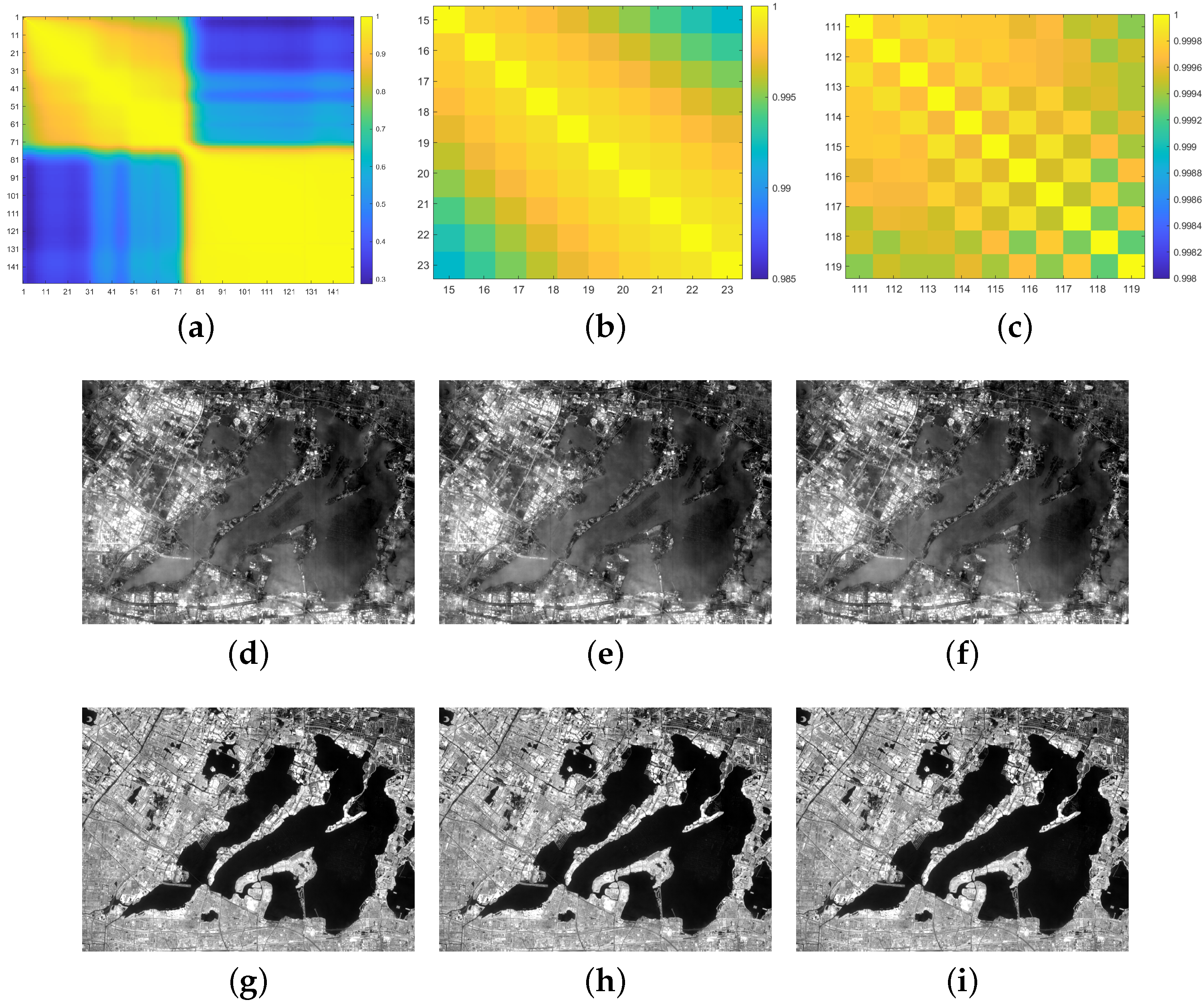
For the YC Lake data with 150 bands, (a): the correlation coefficient image between the spectral bands with a size of ; (b): the correlation coefficient image of Band 15–24; (c): the correlation coefficient image of Band 111–120; (d–i): the gray image for Band 19–21, 113–115. The corresponding correlation coefficient between Band i and j (denoted ) are attached: , , , , .
Figure 7.
For the YC Lake data with 150 bands, (a): the correlation coefficient image between the spectral bands with a size of ; (b): the correlation coefficient image of Band 15–24; (c): the correlation coefficient image of Band 111–120; (d–i): the gray image for Band 19–21, 113–115. The corresponding correlation coefficient between Band i and j (denoted ) are attached: , , , , .

Figure 8.
For the YC Lake data with 150 bands, (a–f): the CEM results for different Ls (L = 5, 10, 40, 50, 100, 150); (g): the CEM result with the skewness selection process, and ; (h): the ROC curves with different Ls.
Figure 8.
For the YC Lake data with 150 bands, (a–f): the CEM results for different Ls (L = 5, 10, 40, 50, 100, 150); (g): the CEM result with the skewness selection process, and ; (h): the ROC curves with different Ls.

Figure 9.
For the Indian Pines data with 200 bands, (a) the false color image (R:Band 44, G:Band 31, B:Band 18); (b): groundtruth data with 16 classes; (c): the groundtruth image for the 16th class; (d): the selected spectrum of the target.
Figure 9.
For the Indian Pines data with 200 bands, (a) the false color image (R:Band 44, G:Band 31, B:Band 18); (b): groundtruth data with 16 classes; (c): the groundtruth image for the 16th class; (d): the selected spectrum of the target.

Figure 10.
For the Indian Pines data, (a): the CEM result with 25 bands via down-sampling by averaging the data with 200 bands; (b): the CEM result with 400 bands generated by GCEM; (c): the CEM result for the data with the skewness selection process, and ; (d): the ROC curves with different Ls.
Figure 10.
For the Indian Pines data, (a): the CEM result with 25 bands via down-sampling by averaging the data with 200 bands; (b): the CEM result with 400 bands generated by GCEM; (c): the CEM result for the data with the skewness selection process, and ; (d): the ROC curves with different Ls.


Table 1.
For the simulation data with 3 bands, the comparison of the average filter output energy and the absolute value of the skewness using different Ls.
Table 1.
For the simulation data with 3 bands, the comparison of the average filter output energy and the absolute value of the skewness using different Ls.
| Band Number | ||
|---|---|---|
| Energy | 0.2048 | 0.1228 |
| Skewness | 1.3956 | 0.6810 |
Table 2.
Illustration of the confusion matrix of a binary classification.
| Target | Non-Target | |
|---|---|---|
| Hypothesized Target | True positive (TP) | False positive (FP) |
| Hypothesized Non-target | False negative (FN) | True negative (TN) |
Table 3.
The quantitative comparison for AUC, OA, F-score (denoted ), and Kappa coefficient (denoted ) with different Ls for the Xi’an data. Bold numbers indicate the highest values in each row.
Table 3.
The quantitative comparison for AUC, OA, F-score (denoted ), and Kappa coefficient (denoted ) with different Ls for the Xi’an data. Bold numbers indicate the highest values in each row.
| L | 4 | 8 | 16 | 32 | 64 | 45 |
|---|---|---|---|---|---|---|
| 0.8300 | 0.9429 | 0.9407 | 0.9422 | 0.9503 | 0.9557 | |
| 0.7849 | 0.8905 | 0.8757 | 0.8816 | 0.9191 | 0.9253 | |
| 0.7679 | 0.8850 | 0.8737 | 0.8788 | 0.9148 | 0.9231 | |
| 0.5697 | 0.7809 | 0.7513 | 0.7632 | 0.8382 | 0.8507 |
Table 4.
The quantitative comparison for AUC, OA, F-score (denoted ), and Kappa coefficient (denoted ) with different Ls for the YC Lake data. Bold numbers indicate the highest values in each row.
Table 4.
The quantitative comparison for AUC, OA, F-score (denoted ), and Kappa coefficient (denoted ) with different Ls for the YC Lake data. Bold numbers indicate the highest values in each row.
| L | 5 | 10 | 30 | 50 | 75 | 150 | 83 |
|---|---|---|---|---|---|---|---|
| 0.9628 | 0.9654 | 0.9790 | 0.9799 | 0.9834 | 0.9811 | 0.9844 | |
| 0.9066 | 0.9103 | 0.9353 | 0.9355 | 0.9401 | 0.9361 | 0.9416 | |
| 0.9074 | 0.9105 | 0.9353 | 0.9354 | 0.9398 | 0.9358 | 0.9416 | |
| 0.8133 | 0.8206 | 0.8707 | 0.8710 | 0.8802 | 0.8722 | 0.8831 |
Table 5.
The classes’ names and the number of sample for the Indian Pine data.
| No. | Class | Samples |
|---|---|---|
| 1 | Alfalfa | 46 |
| 2 | Corn-notill | 1428 |
| 3 | Corn-mintill | 830 |
| 4 | Corn | 237 |
| 5 | Grass-pasture | 483 |
| 6 | Grass-trees | 730 |
| 7 | Grass-pasture-mowed | 28 |
| 8 | Hay-windrowed | 478 |
| 9 | Oats | 20 |
| 10 | Soybean-notill | 972 |
| 11 | Soybean-mintill | 2455 |
| 12 | Soybean-clean | 593 |
| 13 | Wheat | 205 |
| 14 | Woods | 1265 |
| 15 | Buildings-Grass-Trees-Drives | 386 |
| 16 | Stone-Steel-Towers | 93 |
| Total | 10,249 |
Table 6.
The quantitative comparison for AUC, OA, F-score (denoted ), and Kappa coefficient (denoted ) with different Ls for the Indian Pine data. Bold numbers indicate the highest values in each row.
Table 6.
The quantitative comparison for AUC, OA, F-score (denoted ), and Kappa coefficient (denoted ) with different Ls for the Indian Pine data. Bold numbers indicate the highest values in each row.
| L | 25 | 400 | 193 |
|---|---|---|---|
| 0.9972 | 0.9611 | 0.9989 | |
| 0.9755 | 0.9591 | 0.9863 | |
| 0.9754 | 0.9582 | 0.9862 | |
| 0.9511 | 0.9183 | 0.9726 |
Publisher’s Note: MDPI stays neutral with regard to jurisdictional claims in published maps and institutional affiliations. |
© 2021 by the authors. Licensee MDPI, Basel, Switzerland. This article is an open access article distributed under the terms and conditions of the Creative Commons Attribution (CC BY) license (https://creativecommons.org/licenses/by/4.0/).
Share and Cite
MDPI and ACS Style
Geng, X.; Wang, L.; Ji, L. Identify Informative Bands for Hyperspectral Target Detection Using the Third-Order Statistic. Remote Sens. 2021, 13, 1776. https://0-doi-org.brum.beds.ac.uk/10.3390/rs13091776
AMA Style
Geng X, Wang L, Ji L. Identify Informative Bands for Hyperspectral Target Detection Using the Third-Order Statistic. Remote Sensing. 2021; 13(9):1776. https://0-doi-org.brum.beds.ac.uk/10.3390/rs13091776
Chicago/Turabian StyleGeng, Xiurui, Lei Wang, and Luyan Ji. 2021. "Identify Informative Bands for Hyperspectral Target Detection Using the Third-Order Statistic" Remote Sensing 13, no. 9: 1776. https://0-doi-org.brum.beds.ac.uk/10.3390/rs13091776
Note that from the first issue of 2016, this journal uses article numbers instead of page numbers. See further details here.