Enhanced Pulsed-Source Localization with 3 Hydrophones: Uncertainty Estimates

Abstract

The uncertainty behavior of an enhanced three-dimensional (3D) localization scheme for pulsed sources based on relative travel times at a large-aperture three-hydrophone array is studied. The localization scheme is an extension of a two-hydrophone localization approach based on time differences between direct and surface-reflected arrivals, an approach with significant advantages, but also drawbacks, such as left-right ambiguity, high range/depth uncertainties for broadside sources, and high bearing uncertainties for endfire sources. These drawbacks can be removed by adding a third hydrophone. The 3D localization problem is separated into two, a range/depth estimation problem, for which only the hydrophone depths are needed, and a bearing estimation problem, if the hydrophone geometry in the horizontal is known as well. The refraction of acoustic paths is taken into account using ray theory. The condition for existence of surface-reflected arrivals can be relaxed by considering arrivals with an upper turning point, allowing for localization at longer ranges. A Bayesian framework is adopted, allowing for the estimation of localization uncertainties. Uncertainty estimates are obtained through analytic predictions and simulations and they are compared against two-hydrophone localization uncertainties as well as against two-dimensional localization that is based on direct arrivals.

1. Introduction

Underwater pulsed-source localization is of importance for a broad range of marine operations, from the monitoring of underwater vehicles [1], search and rescue operations [2], to wildlife monitoring [3,4], and spatial audio applications [5]. For this purpose, arrays of synchronized hydrophones are commonly used, such that relative arrival times, so-called time differences of arrival (TDOAs), can be estimated.

The minimum number of hydrophones required for three-dimensional (3D) localization is four when direct arrivals (one arrival per hydrophone) are considered [6]. In many cases, direct arrivals are followed by arrivals that are associated with acoustic paths reflected off the sea surface and/or the sea bottom. While the surface-reflected arrivals are typical in deep water environments [7], surface- and bottom-reflected arrivals are observed in shallow waters [8].

If direct and surface-reflected arrivals are exploited, 3D localization can be obtained, even with two hydrophones. Hydrophone pairs, usually towed behind a vessel, have broadly been used for bearing estimation from direct arrivals [9]. Various 3D localization approaches exploiting direct and surface-reflected arrivals at two hydrophones have been proposed for homogeneous environments [10,11,12], as well as for refractive environments [13,14,15,16]. In [16], the two-hydrophone localization problem was embedded in a Bayesian framework, enabling the estimation of localization uncertainties that are caused by errors in the TDOAs and hydrophone locations, as well as by uncertainties in the sound-speed profile characterizing a refractive environment. This approach was applied to a series of controlled localization experiments as well as for the localization of sperm whales in the Eastern Mediterranean Sea using a large-aperture towed hydrophone array [17].

A significant point in [16,17] is that the 3D localization problem can be separated into two problems, one of range/depth estimation, for which only the hydrophone depths are needed, and one of bearing estimation, if the hydrophone locations in the horizontal are also known. This is a significant advantage for hydrophones towed or suspended from surface platforms, since the hydrophone depths can be obtained much easier (e.g., from depth sensors) than their location in the horizontal. On the other hand, the two-hydrophone 3D localization approach suffers from certain drawbacks, such as left-right ambiguity, high range/depth uncertainties for source locations close to the array broadside, and high bearing uncertainties for source locations that are close to the endfire. These drawbacks can be removed by adding a third hydrophone, not aligned with the other two, such as to break the symmetry and increase directional diversity.

Several authors have proposed methods for 3D localization with three or more hydrophones using direct arrivals and, in some cases, reflected arrivals [6,7,8,18]. The most common approach is through the intersection of hyperboloids corresponding to the TDOAs between direct arrivals at the different hydrophone pairs [19,20,21,22], which can be regarded as a generalization of methods for bearing estimation [9,23]. Several of these works refer to large-aperture arrays of synchronized hydrophones with separations between 0.5 and 3 km. Networks of asynchronous compact (tetrahedral) arrays have also been proposed [24,25,26], allowing for 3D localization through triangulation or, alternatively, through back-propagation by exploiting surface-reflected arrivals at a single node [26]. Networks of asynchronous free-drifting acoustic stations with suspended hydrophone pairs have been used for localization exploiting direct and surface-reflected arrivals [27,28], whereas combinations of different types of receiving stations (single hydrophones, vertical line arrays, and compact hydrophone arrays) have also been used [29,30]. For the estimation of localization uncertainties that are caused by measurement errors and parameter ambiguities various error propagation methods have been applied [6,7,21]. The application of a Bayesian framework has enabled an integrated approach to the localization and uncertainty quantification problem [8,16,17,31,32,33].

In this work, an enhanced three-hydrophone 3D localization method is presented, which extends and enhances the two-hydrophone approach based on direct and surface-reflected arrivals [16]. The proposed method adopts the Bayesian framework for the estimation of localization uncertainties, takes refraction of acoustic paths using ray theory into account, and exploits rays with an upper turning point, achieving localization at longer ranges. The 3D localization problem is solved in two steps, first the range/depth estimation problem is addressed relying on known hydrophone depths, followed by the localization in the horizontal if the hydrophone geometry in the horizontal is also known. Uncertainty distributions, obtained through linearized, analytic predictions, are compared against two-hydrophone localization uncertainties [16] and against empirical distributions from full non-linear inversions. Comparisons against a two-dimensional (2D) localization approach, based on direct arrivals [6], are also presented. Three different array geometries are considered, being associated with the design of a moored acoustic observatory for sperm whales, planned to be deployed in summer 2021 in deep water, south of the island of Crete in the Eastern Mediterranean Sea, in the framework of the SAvEWhales project.

The contents of the work are organized, as follows: Section 2 presents the general Bayesian estimation framework for range/depth estimation (Section 2.1.1) and localization in the horizontal (Section 2.1.2). These two steps comprise the 3D localization approach, in which both direct and surface-reflected arrivals are exploited. Section 2.2 addresses 2D localization in the horizontal relying on direct arrivals only. Section 3 presents the numerical results for localization uncertainties that are based on analytic estimates and simulations. It also presents some comparisons to uncertainties from two-hydrophone localization as well as from 2D localization based on direct arrivals. Section 4 discusses the main results and, finally, the basic conclusions are drawn in Section 5.

2. Bayesian Inversion Framework

In this section, the general Bayesian inversion framework is described and, then, in the following subsections, it is adapted to the specific localization problems of interest. Let $\mathbf{d}$ be a data vector, i.e., a vector containing any observable (measured) quantities, and $\mathbf{m}$ a model vector containing the sought (unknown) parameters. The model relation expressing the data vector in terms of the model vector is formulated as

$$\mathbf{d}=\mathbf{F}\left(\mathbf{m}\right).$$

(1)

This relation is non-linear, in general, but it can be linearized by applying a Taylor series expansion [34] regarding a reference model state, ${\mathbf{m}}_l$,

$$\mathbf{d}={\mathbf{d}}_l+{\mathbf{J}}_l\left(\mathbf{m}-{\mathbf{m}}_l\right),$$

(2)

where ${\mathbf{d}}_l=\mathbf{F}\left({\mathbf{m}}_l\right)$ and ${\mathbf{J}}_l$ is the Jacobian matrix of $\mathbf{F}(·)$ evaluated at the linearization reference ${\mathbf{m}}_l$, i.e., ${\mathbf{J}}_{l,ij}=\partial F_i\left({\mathbf{m}}_l\right)/\partial m_j$. The data vector is subject to measurement errors and it can be written as ${\displaystyle \mathbf{d}={\mathbf{d}}_m+\delta \mathbf{d}}$, where ${\mathbf{d}}_m$ is the measured data vector and $\delta \mathbf{d}$ is the vector of measurement errors, which are assumed to be uncorrelated and normally distributed zero-mean random variables, characterized by a diagonal covariance matrix ${\mathbf{C}}_d$. Exploiting prior information, the model vector can be regularized assuming a normal distribution about an a priori mean ${\mathbf{m}}_p$, i.e., ${\displaystyle \mathbf{m}={\mathbf{m}}_p+\delta \mathbf{m}.}$ Assuming uncorrelated prior regularization constraints, the covariance matrix ${\mathbf{C}}_p$ of $\delta \mathbf{m}$ will also be diagonal.

The posterior probability density of the model vector, $\mathbf{m}$, given the measured data vector, ${\mathbf{d}}_m$, according to Bayes’ theorem [35] for the linear problem that is described in Equation (2) takes the form

$$\begin{array}{cc}\hfill p_{\mathbf{m}|\mathbf{d}}\left(\mathbf{m}|{\mathbf{d}}_m\right)& =\frac{p_{\mathbf{d}|\mathbf{m}}\left({\mathbf{d}}_m|\mathbf{m}\right)p_{\mathbf{m}}\left(\mathbf{m}\right)}{p_{\mathbf{d}}\left({\mathbf{d}}_m\right)}\hfill \\ \hfill & \propto exp\left\{-\frac{1}{2}{\left({\mathbf{d}}_m-{\mathbf{d}}_l-{\mathbf{J}}_l\left(\mathbf{m}-{\mathbf{m}}_l\right)\right)}^T\right.\times {\mathbf{C}}_d^{-1}\left({\mathbf{d}}_m-{\mathbf{d}}_l-{\mathbf{J}}_l\left(\mathbf{m}-{\mathbf{m}}_l\right)\right)\hfill \\ \hfill & \left.-\frac{1}{2}{\left(\mathbf{m}-{\mathbf{m}}_p\right)}^T{\mathbf{C}}_p^{-1}\left(\mathbf{m}-{\mathbf{m}}_p\right)\right\}.\hfill \end{array}$$

(3)

The maximum a posteriori solution is then provided by the value maximizing the above expression [36]

$$\begin{array}{cc}\hfill \widehat{\mathbf{m}}={\mathbf{m}}_p& +{\left({\mathbf{J}}_l^T{\mathbf{C}}_d^{-1}{\mathbf{J}}_l+{\mathbf{C}}_p^{-1}\right)}^{-1}{\mathbf{J}}_l^T{\mathbf{C}}_d^{-1}\times \left({\mathbf{d}}_m-{\mathbf{d}}_l-{\mathbf{J}}_l\left({\mathbf{m}}_p-{\mathbf{m}}_l\right)\right).\hfill \end{array}$$

(4)

The corresponding posterior covariance matrix of $p_{\mathbf{m}|\mathbf{d}}\left(\mathbf{m}|{\mathbf{d}}_m\right)$ is given by the expression

$${\mathbf{C}}_m={\left({\mathbf{J}}_l^T{\mathbf{C}}_d^{-1}{\mathbf{J}}_l+{\mathbf{C}}_p^{-1}\right)}^{-1}.$$

(5)

The square root of the diagonal elements of ${\mathbf{C}}_m$ provides the posterior root-mean-square (RMS) uncertainties of the model parameters.

In the following subsections, the above Bayesian inversion framework is adapted to each of the two steps of the 3D localization problem. In the first step, the three source ranges (source distances from the three hydrophones) and the source depth are estimated from the TDOAs at the three hydrophones. For this step, only the hydrophone depths need to be known. If the hydrophone locations in the horizontal are as well known, then, in the second step, these are combined with the estimated source ranges from the first step to estimate the source location in the horizontal. Thus, the 3D source location, i.e., range, depth, and bearing, can be estimated. In the last part of this section, a simpler 2D localization method omitting the depth dimension is described, relying on the two TDOAs between direct arrivals at the three hydrophones.

2.1. 3D Localization

2.1.1. Step 1: Range/Depth Estimation

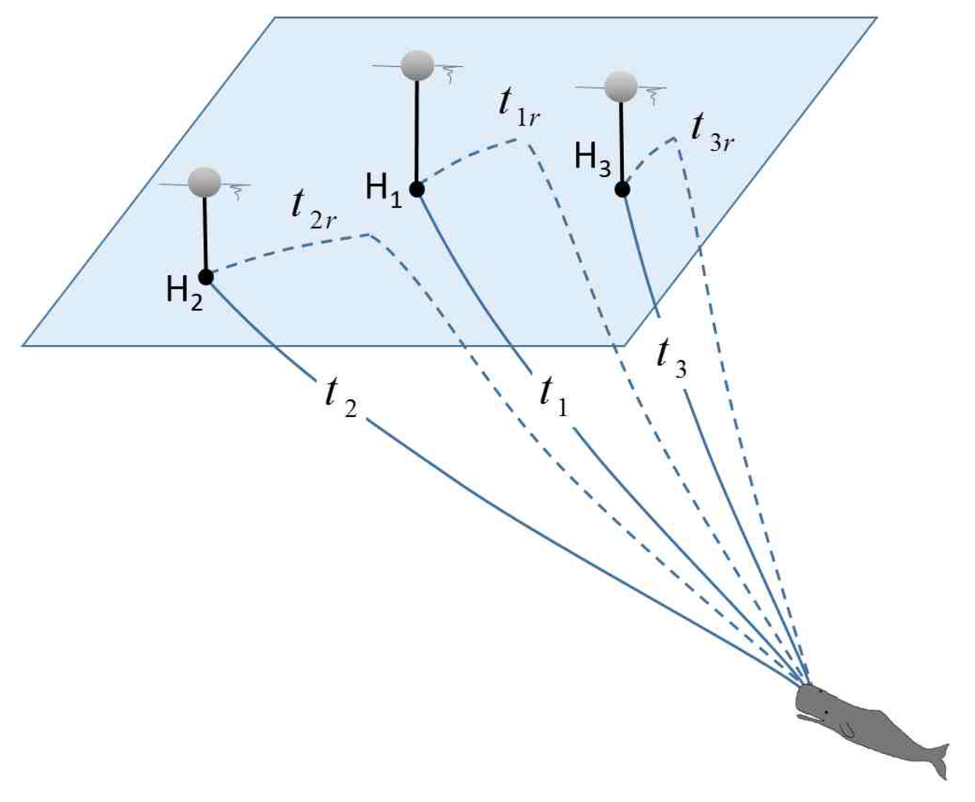
An array of three synchronized hydrophones, H${}_1$, H${}_2$, and H${}_3$, at known depths in a refractive environment characterized by a depth-dependent, range-independent sound–speed profile, is assumed. Direct and surface-reflected acoustic arrivals from a pulsed source of unknown location are picked up by the hydrophones, as shown in Figure 1. By utilizing the TDOAs between direct and surface-reflected arrivals at each hydrophone and between direct arrivals at the different hydrophones, the three source ranges (distances from the three hydrophones) as well as the source depth can be estimated.

Let $t_1$ denote the travel time of the pulsed signal from the source to hydrophone H${}_1$ over the direct path and $t_{1r}$ the travel time over the surface-reflected path. Similarly, $t_2$, $t_{2r}$, $t_3$, and $t_{3r}$ are the corresponding travel times to hydrophones H${}_2$ and H${}_3$, respectively. Subsequently, five TDOAs can be defined, resulting in the following data vector

$$\mathbf{d}={\left[{\tau }_{1r1},{\tau }_{2r2},{\tau }_{3r3},{\tau }_{21},{\tau }_{31}\right]}^T,$$

(6)

where ${\tau }_{1r1}=t_{1r}-t_1$, ${\tau }_{2r2}=t_{2r}-t_2$, ${\tau }_{3r3}=t_{3r}-t_3$, ${\tau }_{21}=t_2-t_1$, and ${\tau }_{31}=t_3-t_1$.

The model vector includes the source ranges (horizontal distances between the source and each of the three hydrophones), $r_1$, $r_2$, and $r_3$, the source depth, $z_s$, as well as the hydrophone depths, $h_1,h_2,h_3$, and a sound-speed parameter, $\theta$ representing the variability in the sound speed profile,

$$\mathbf{m}={\left[r_1,r_2,r_3,z_s,h_1,h_2,h_3,\theta \right]}^T.$$

(7)

The last four quantities, $h_1,h_2,h_3$, and $\theta$, are included, such that the influence of the corresponding inaccuracies on the localization uncertainties can be accounted for. The actual sound-speed profile, $c\left(z\right)$, is assumed to be a perturbation of the measured sound-speed profile, $c_m\left(z\right)$

$$c\left(z\right)=c_m\left(z\right)+\theta g\left(z\right),$$

(8)

where $g\left(z\right)$ is a depth-dependent perturbation mode (vertical mode) and the parameter $\theta$ is assumed to be a Gaussian, zero-mean random variable. The mode $g\left(z\right)$ and the parameter $\theta$ represent the anticipated divergence from the measured sound-speed profile.

The Jacobian matrix expresses the sensitivity of the data vector, i.e., the TDOAs, to changes in the model vector, $\mathbf{m}$, i.e., changes in the source ranges and depth, the hydrophone depths, and the sound-speed parameter, $\theta$. The expressions for the derivatives of the travel times and their analytical derivation can be found in [16].

The above approach relies on TDOAs between the direct and surface-reflected arrivals. In a homogeneous environment (constant sound speed), surface-reflected arrivals will always be available for any source range and depth. However, in the case of strong near-surface sound-speed gradients, e.g., due to rapid temperature increase towards the surface, refraction may prevent a ray from reaching the surface, especially for sources at longer ranges. In that case, the source signal reaches the receiver over a direct path and a path that has an upper turning point rather than a surface reflection. In this connection, the dashed-line eigenrays that are shown in Figure 1 may be thought of either as surface-reflected rays or rays with an upper turning point. Rays with upper turning points can alternatively be used in place of surface-reflected rays for source range/depth estimation. The extension to turning-point eigenrays enables the localization of sources at longer ranges and, in this connection, it is of practical interest, as will become clear in Section 3.

With the above definitions and expressions, the solution of the linearized range/ depth estimation problem can be obtained from Equations (4) and (5). An iterative scheme is applied to address the non-linearity of the model relations: using a first guess for $r_1$, $r_2$, $r_3$, $z_s$, and their standard deviations, the model relations are linearized about the selected source range/depth values, the measured hydrophone depths and the measured sound-speed profile ($\theta =0$), and the linear inverse problem is solved (Equations (4) and (5)). Subsequently, each next step in the iteration process uses the inversion results from the previous step as linearization reference. For $r_1$, $r_2$, $r_3$, and $z_s$, the inversion results are also used as prior means, whereas the initial standard deviations are gradually increased such as to remove the corresponding constraints. For $h_1$, $h_2$, $h_3$ and $\theta$ the measured values and corresponding standard deviations are used as a priori constraints for all inversions. For a robust estimation, the final localization, after convergence, has to be independent of the initial guess.

2.1.2. Step 2: Localization in the Horizontal

If the hydrophone locations in the horizontal are known, they can be combined with the estimated ranges, $r_1,r_2,r_3$ from the previous section to specify the horizontal location of the source. Adopting a cartesian coordinate system $\left(x,y\right)$, the assumed receiver locations are denoted by $\left(x_1,y_1\right), \left(x_2,y_2\right), \left(x_3,y_3\right)$ and the sought source location by $\left(x_s,y_s\right)$. Subsequently, the following equations hold:

$$\begin{array}{c}\hfill {\left(x_s-x_i\right)}^2+{\left(y_s-y_i\right)}^2=r_i^2,i=1,2,3.\end{array}$$

(9)

This is an overdetermined system of equations for $\left(x_s,y_s\right)$ with data vector

$$\mathbf{d}={\left[r_1,r_2,r_3\right]}^T,$$

(10)

and model vector

$$\mathbf{m}={\left[x_s,y_s,x_1,y_1,x_2,y_2,x_3,y_3\right]}^T.$$

(11)

In this case, the data covariance matrix is the upper-left 3 × 3 submatrix of the posterior covariance matrix from the previous step, which is not diagonal in general. The individual terms of the Jacobian (i.e., the derivatives of $r_i$ with respect to $x_s$, $y_s$, $x_i$, and $y_i$, $i=1,2,3$) can be easily derived from Equation (9). Equations (4) and (5) give the solution to the linear problem. To deal with the non-linearity of the model relations, Equation (9), an iterative approach is applied, initiated by a first guess for $x_s$, $y_s$, and their standard deviations, in a similar way as in the previous section. Section 3.1.2 gives examples of this iterative scheme.

2.2. 2D Localization

In the previous Section 2.1, the estimation of source range, depth, and horizontal location is achieved by exploiting the TDOAs between double arrivals (direct and surface-reflected arrivals or direct and turning-point arrivals) at the three hydrophones. However, there are cases where double arrivals may not be available, e.g., the surface-reflected arrivals may be weak due to increased surface roughness, or the delay from the leading direct arrivals may be too small to resolve, e.g., if the source is too close to the surface. In such situations, an approximate 2D localization in the horizontal can be carried out based on the direct arrivals only, omitting the depth dimension of the problem, assuming known hydrophone locations in the horizontal [6].

In this case, the data vector, based on TDOAs between direct arrivals, is defined as

$$\mathbf{d}={\left[{\tau }_{21},{\tau }_{31}\right]}^T,$$

(12)

and the model vector as

$$\mathbf{m}={\left[x_s,y_s,x_1,y_1,x_2,y_2,x_3,y_3\right]}^T.$$

(13)

In the absence of the depth dimension, the model relations can be expressed as

$$\begin{array}{ll}{\tau }_{i1}& =\left[\sqrt{{\left(x_s-x_i\right)}^2+{\left(y_s-y_i\right)}^2}\right.\\ & \left.-\sqrt{{\left(x_s-x_1\right)}^2+{\left(y_s-y_1\right)}^2}\right]/c,i=2,3,\end{array}$$

(14)

where c is a typical sound-speed value (e.g., 1500 m/s). The Jacobian terms are simply the derivatives of these expressions with respect to $x_s$, $y_s$, $x_i$, and $y_i$, $i=1,2,3$. While the Jacobian can be used for the calculation of the localization uncertainties, Equation (5), the location estimates, ${\widehat{x}}_s$, and ${\widehat{y}}_s$, themselves can be directly obtained by triangulation.

3. Numerical Results

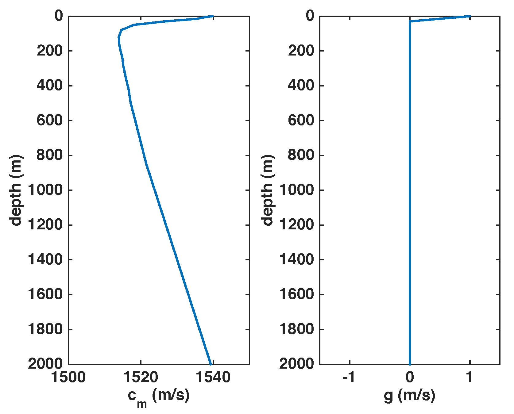
Some numerical results for localization uncertainties that are based on analytic estimates and simulations are presented in this section. The same sound-speed profile and vertical sound-speed mode are assumed, as in [16], shown in Figure 2, representing typical propagation conditions for the eastern Mediterranean Sea in summer. The sound speed mode is linearly increasing from 0 m/s at a depth of 30 m to 1 m/s at the surface, representing sound speed deviations due to warming/cooling of the near the surface layer. The source is assumed at a depth of 800 m, a typical foraging depth for sperm whales, and at different ranges and azimuths.

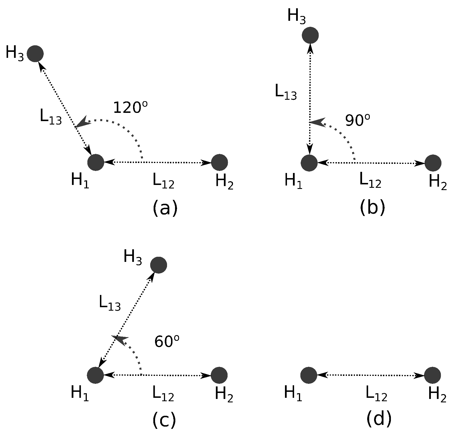
All three hydrophones are assumed at a depth of 100 m forming an isosceles triangle with side length $L_{12}=L_{13}=$1000 m and central angle of 120°, 90°, and 60°, i.e., an obtuse, right, and equilateral triangle, respectively, as shown in Figure 3. For comparison purposes a two-hydrophone array, Figure 3d, is also considered.

The RMS error for TDOAs between direct arrivals at different hydrophones, assuming high-accuracy synchronization, e.g., through pulse-per-second (PPS) signals [37], is taken $\delta {\tau }_{21,\mathrm{RMS}}=\delta {\tau }_{31,\mathrm{RMS}}=0.1$ ms. The surface-reflected travel times are subject to additional errors due to the sea-surface roughness [38] and, in this connection, a larger value is taken for the RMS error for TDOAs between direct and surface-reflected arrivals, $\delta {\tau }_{iri,\mathrm{RMS}}=0.2$ ms, $i=1,2,3$ [17]. The RMS uncertainty for the hydrophone depths is taken $\delta h_{i,\mathrm{RMS}}=0.1$ m, $i=1,2,3$, being compatible with typical accuracies of depth sensors ($\pm 0.1$ to $\pm 0.2\%$ of the full scale, the latter assumed 100 m) and for the sound-speed parameter ${\theta }_{\mathrm{RMS}}=1$ corresponding to an RMS error in the temperature measurement at the sea surface of about 0.45 °C.

3.1. 3D Localization Uncertainty

Localization uncertainties for the two steps of the 3D localization approach, range/ depth estimation, and localization in the horizontal are presented in this section. Further, some comparisons with two-hydrophone localization uncertainties are carried out.

3.1.1. Range/Depth Estimation

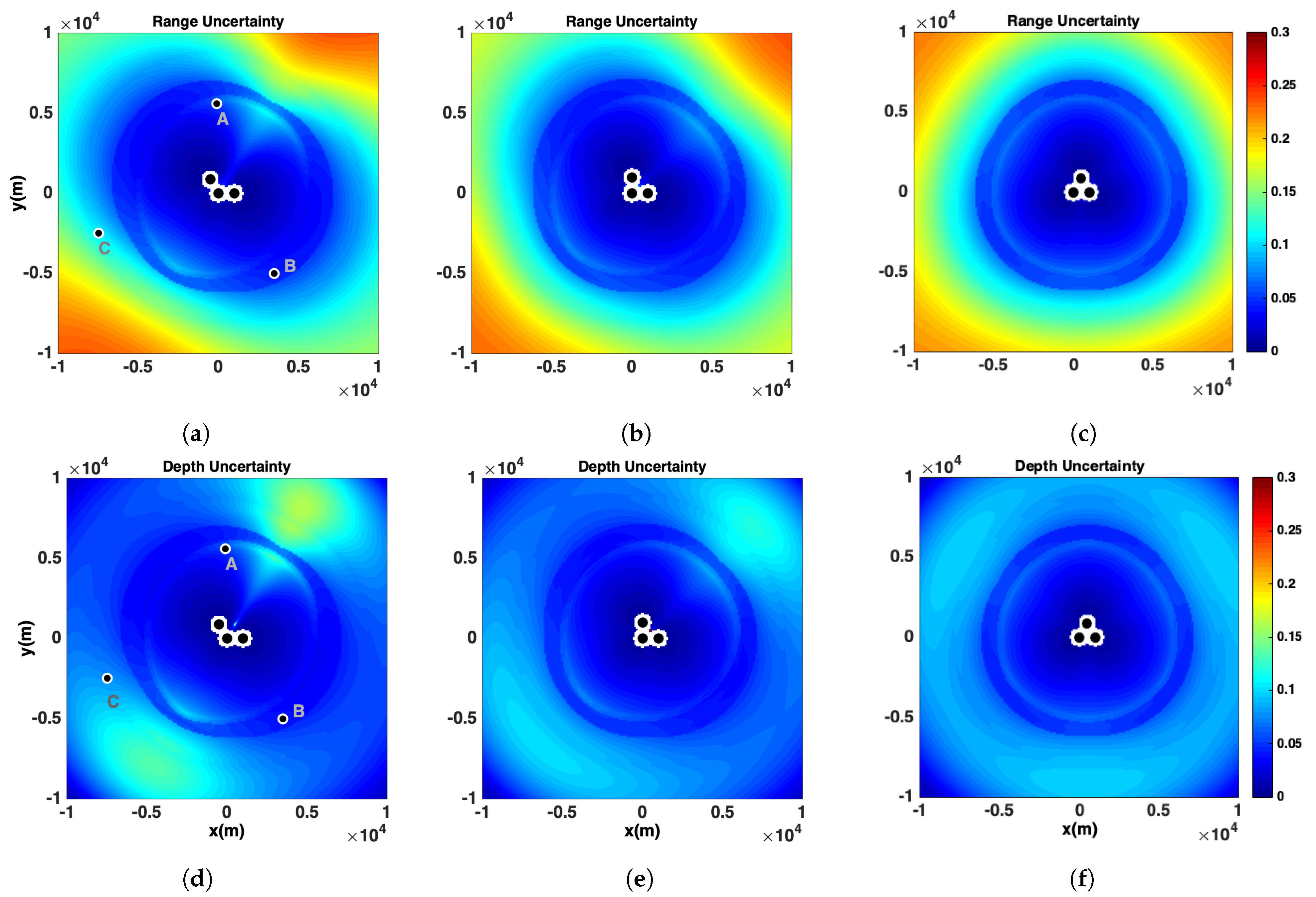
Figure 4 presents the analytic source range and depth uncertainty distributions for the three array geometries considered, for different source locations in the horizontal (x-y plane), covering a 20 km × 20 km area about each array. The top three panels show the RMS uncertainty in range, and the bottom three panels the RMS uncertainty in depth, both being normalized with the actual value of the respective quantity (actual range or depth). The normalized range uncertainty increases with distance from the array, taking larger values at the broadside of the hydrophone pair with the largest separation. As expected, the uncertainty distribution becomes more uniform in azimuth as the array geometry changes from obtuse to right and, finally, equilateral. The maximum range uncertainties remain smaller than 25% for all source locations. The normalized depth uncertainty also increases with distance up to a certain range, beyond which it starts to decrease—this behavior will be explained shortly—remaining smaller than $15\%$. Again, the uncertainties are larger at the broadside of the hydrophone pair with the largest separation and become azimuthally more uniform in the case of the equilateral array geometry.

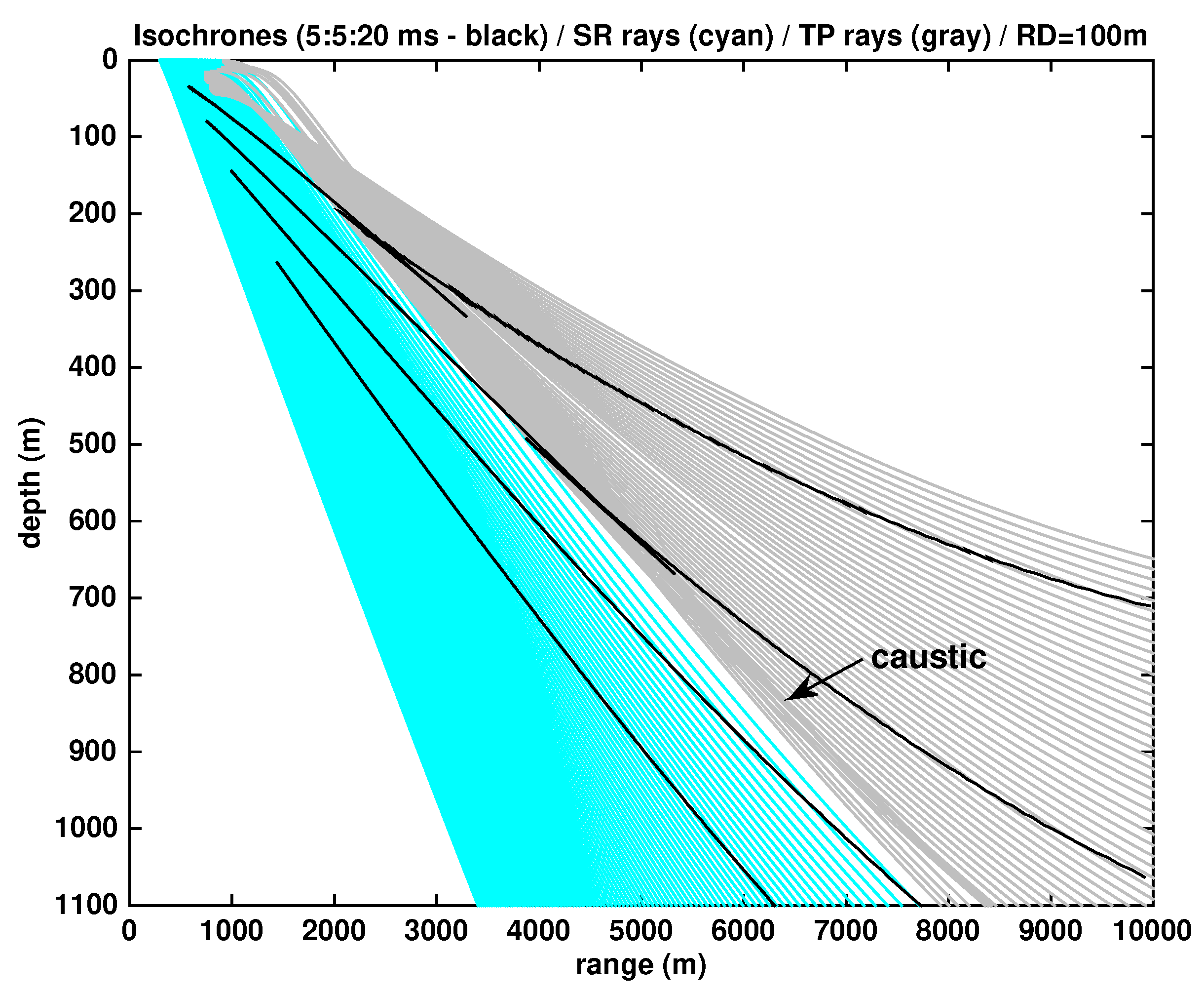
At a range of approximately 6 km, a ring formation is observed in Figure 4, characterized by a slightly different uncertainty behavior for all three array types, both in range and depth. This ring is associated with the existence of caustics and, in this connection, it is called “the caustics zone”. Figure 5 shows the geometries of surface-reflected and turning-point rays (cyan and gray lines, respectively) emanating from a receiver on the vertical axis at a depth of 100 m in the refractive environment that is characterized by the sound-speed profile of Figure 2. Only the parts of the rays from the corresponding surface-reflection/turning point outward are shown. Rays that have a large grazing angle at the receiver reach the surface and continue as surface-reflected (cyan) rays. At smaller grazing angles after a certain point, the strong downward refraction prevents the rays from reaching the surface and gives rise to an upper turning point, such that the rays are no longer surface-reflected, but refracted (grey) with an upper turning point. Refracted rays have the tendency to form caustics, in which case a decrease of the grazing angle at the receiver causes a temporary contraction, a range decrease, in contrast to the general trend. Such a caustic formation is seen in the first gray rays that are shown in Figure 5.

The isochrones corresponding to 5, 10, 15, and 20 ms are also shown (black lines) in Figure 5. Each isochrone is the locus of points (range-depth pairs), where the TDOA between direct and surface-reflected/turning-point arrivals at the receiver takes a certain value and, thus, it is the locus of possible solutions to the localization (range/depth estimation) problem. The shallowest isochrone presented in Figure 5 corresponds to 5 ms and the deepest one to 20 ms.

Taking the 5-ms isochrone, the following remarks can be made. In general, the depth increases with range, and the gradient of this dependence decreases with range due to refraction. When the isochrone meets the caustic, it suffers a temporary setback during which the range and depth decrease—rather than increase—with decreasing grazing angle at the receiver. This behavior gives rise to local multiplicity in the range-depth dependence, which causes ambiguity in the localization problem [13]. Nevertheless, as it is observed in Figure 5, the deviation of the caustic loop from the main part of the isochrone is relatively small and it becomes smaller for steeper isochrones that correspond to larger TDOA values (deeper sources): the 5-ms isochrone meets the caustic at about 300-m depth and 3300-m range, and the resulting caustic loop is quite well separated from the main isochrone body, whereas the 10-ms isochrone meets the caustic at about 670-m depth and 5400-m range, and the caustic loop is very close to the isochrone body. For a source depth of 800 m, the caustic is encountered at the range of about 6 km, the range where the rings in Figure 4 are observed. The rings result from the superposition of the caustic deviations from the three hydrophones.

The leveling in the shape of the isochrones with increasing range, as observed in Figure 5, explains the difference in the behavior of the uncertainty distribution of the normalized depth, when compared to that of the normalized range for longer ranges in Figure 4, namely the fact that the range uncertainty increases for longer ranges, while the depth uncertainty increases up to a certain point and then decreases. By observing the isochrones presented in Figure 5, it is seen that for a certain source depth, e.g., 800 m, the gradient of the depth dependence on range decreases as the range becomes larger. This change in slope, which is due to refraction, indicates that the uncertainty in depth estimation becomes gradually smaller relative to the uncertainty in range estimation. This is the behavior observed in Figure 4 at longer ranges.

Further, in Figure 5, the extension of the localization range that is obtained through the exploitation of turning-point arrivals can be seen. For example, for source depths of 800 m and 1000 m, the surface-reflected rays in the particular environment reach out to about 5.7 and 7 km, respectively. Assuming that a minimum time difference of 10 ms is required for arrival resolution, the corresponding ranges for turning-point arrivals along the 10-ms isochrone are about 6.7 and 9 km, an extension by about 1 km and 2 km, respectively.

The uncertainty estimates that are shown in Figure 4 are based on local linear approximations of the model relations. In order to check the validity of these linear approximations, Monte Carlo simulations are carried out in the case of the obtuse array geometry for three source locations A, B, and C, as shown in Figure 4a,d. In each simulation, a large number of non-linear inversions are carried out. Each inversion applies on different synthetic data (TDOAs, hydrophone depths, sound-speed parameter) that are generated by adding random errors that are drawn from normal probability density functions (PDFs), the same as those underlying Figure 4. The histograms of the resulting source ranges and depth (posterior empirical distributions) are then compared with the posterior analytic PDFs that result from the analytic approach.

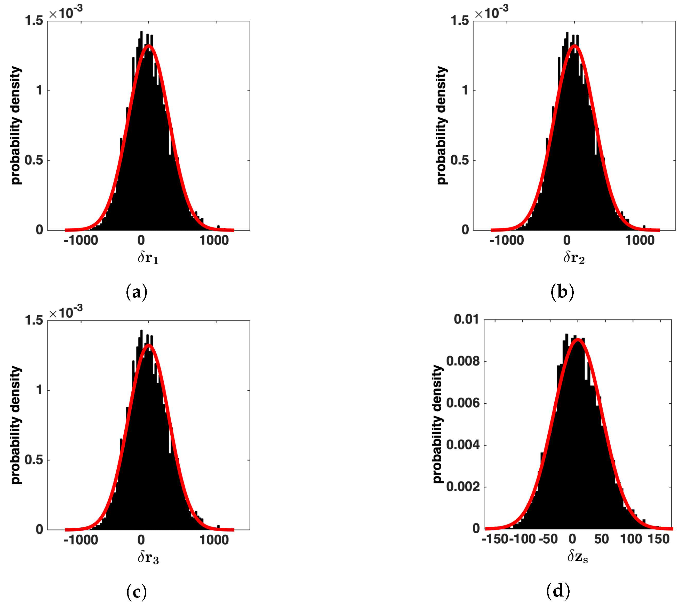
Figure 6 shows the normalized histograms of the deviations of the ranges $r_1$, $r_2$, $r_3$, and depth $z_s$ from their true values ($x_s=-100$ m, $y_s=5600$ m, $z_s=800$ m) for source location A. For the generation of the histograms, 5000 independent non-linear inversions were conducted with randomly perturbed synthetic data. The corresponding normal PDFs (red solid curves) that result from the analytic approach are also shown in this figure. It is seen that all four empirical distributions are in very good agreement with the analytic PDFs indicating that the linearization is a good approximation in this case.

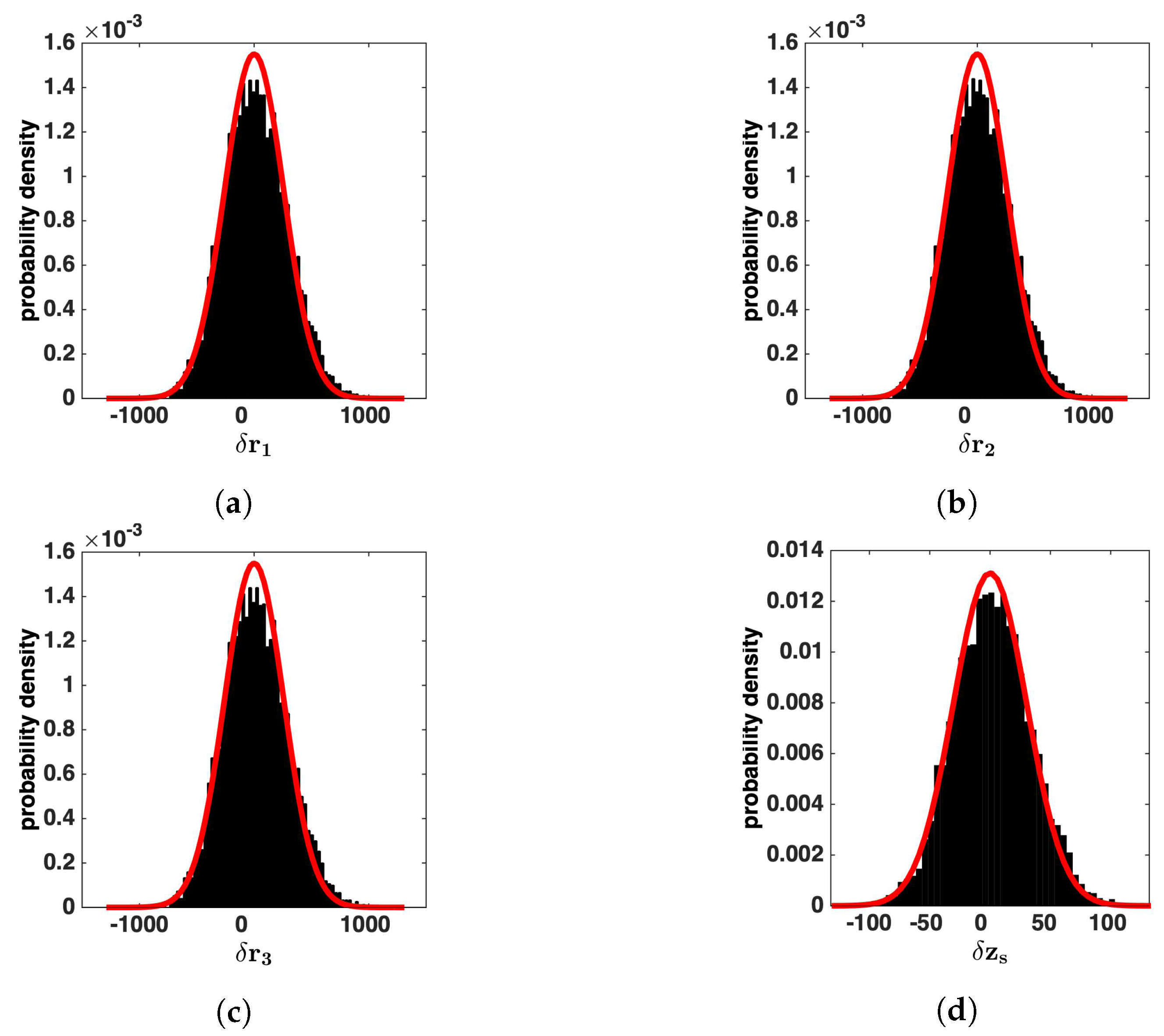
Figure 7 shows the normalized empirical distributions for source location B ($x_s=3500$ m, $y_s=-5000$ m, $z_s=800$ m). In this case, the source lies on the caustics zone. As in the previous case, 5000 non-linear inversions with randomly perturbed synthetic data were used to generate the histograms. Again, the corresponding analytic normal PDFs (red solid curves) from the local linear approach are superimposed. Additionally, for this case, the histograms fit very well the analytic PDFs. It is worth noticing that the depth uncertainty presented in Figure 7d is smaller than in Figure 6d. This is due to the drop in relative uncertainty on the caustics zone, cf. Figure 4d. On the other hand, the range deviations have approximately the same behavior as in the previous case (Figure 6d); this is because the drop in relative uncertainty on the caustics zone, cf. Figure 4a, is compensated by the increase, by about 500 m, in source range, from A to B.

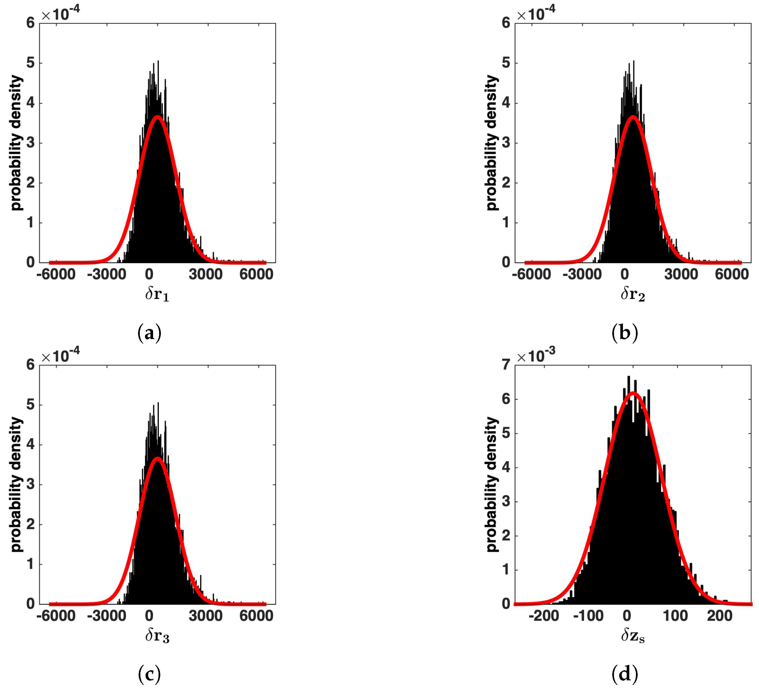
The normalized empirical distribution of range/depth deviations for source location C, from 5000 non-linear inversions with randomly perturbed synthetic data, is shown in Figure 8, along with the corresponding analytic PDFs. Now, the source lies outside the caustics zone at a range of about 7.9 km (true source location $x_s=-7500$ m, $y_s=-2500$ m, $z_s=800$ m), and the empirical distributions are slightly skewed, more for range deviations and less for depth deviations. This is caused by the deviation of the isochrones from linearity and the decrease in their slope at longer ranges, as observed in Figure 5, in a way that affects more the range deviations than the deviations in depth. A further remark is that, while the range uncertainties have increased significantly, by a factor of approximately 3, as compared to the corresponding uncertainties at locations A and B, the increase in the source depth uncertainty is much smaller, approximately by a factor of 1.5; this is associated with the different behavior of range and depth uncertainties that are observed in Figure 4 at longer ranges.

3.1.2. Localization in the Horizontal

The horizontal source location and source bearing can be obtained from the estimated source ranges, provided that the hydrophone geometry in the horizontal is known, to within some uncertainty. In the following, the RMS uncertainty for the horizontal hydrophone fixes is taken $\delta x_{RMS}=\delta y_{RMS}=$10 m.

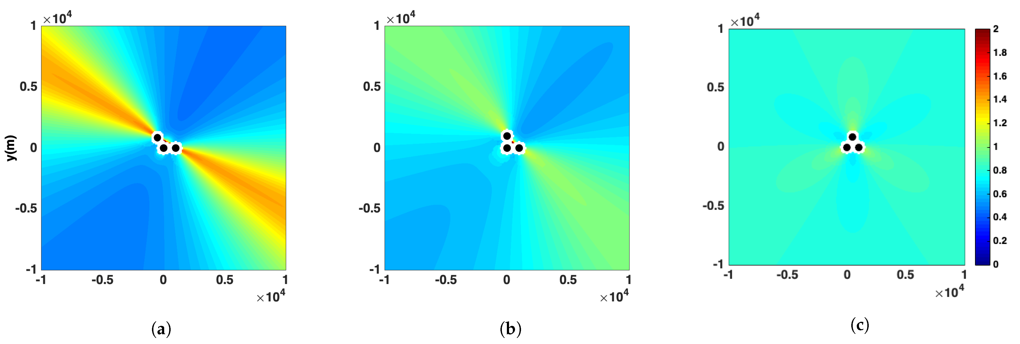
Figure 9 shows the bearing estimation uncertainty distribution for the three array geometries (obtuse, right, and equilateral triangle), relying on the covariance characteristics of the estimated ranges from the previous step. In general, the uncertainty is low, less than $2^{\circ }$, increasing for source locations close to the endfire and decreasing for locations close to the broadside of the hydrophone pair with the largest separation, i.e., the directions aligned with and perpendicular to the longest dimension of the array, respectively. As expected, the uncertainty distribution becomes more uniform as the array geometry changes from obtuse to equilateral. However, in the case of the obtuse array, positions about the endfire exhibit higher error in comparison with the other geometries, whereas, in the broadside area, the obtuse array performs better.

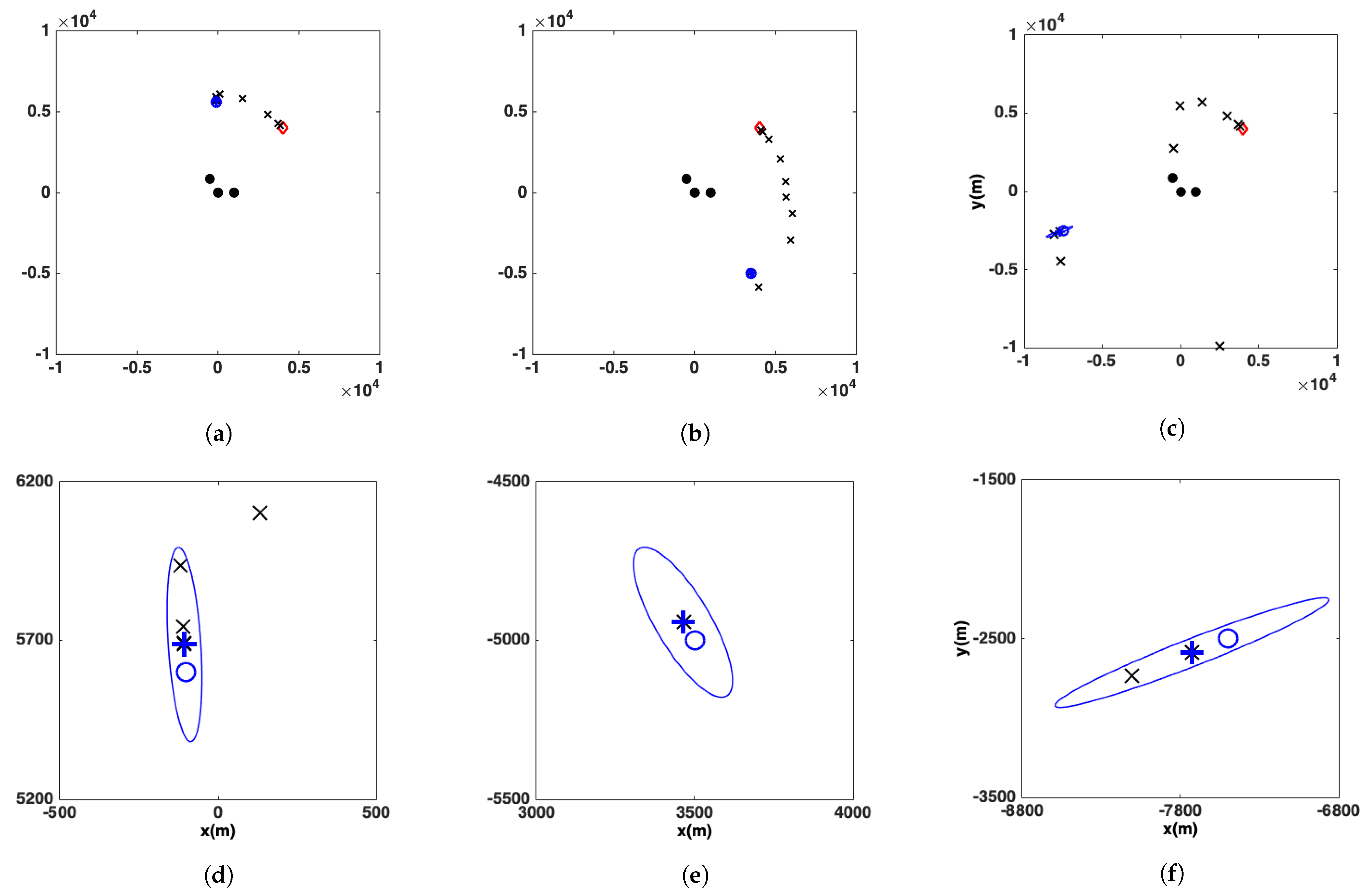
Figure 10 shows three examples for iterative localization in the horizontal in the case of the obtuse array geometry. The three examples correspond to the three source locations, A, B, and C, as shown in Figure 4a,d. For each localization the hydrophone locations are perturbed by adding random errors, drawn from the corresponding prior distributions, to the true hydrophone locations. The prior RMS uncertainties for $x_s$ and $y_s$ for the first iteration step (the first inversion) are set to 10 m, and they are gradually relaxed (doubled) at every subsequent iteration step. The same first guess is used for all three localizations to show that the final localization result is independent from the selection of the first guess once convergence is established. The initial guess, the intermediate, and final localization results are shown in Figure 10 for the three cases, A, B, and C. The uncertainty ellipses about the final localization results that correpond to one standard deviation, resulting from the estimated posterior covariance matrix between $x_s$ and $y_s$ are also shown. In all three cases, the uncertainty in range estimation is in agreement with the results that are shown in Figure 4a. Furthermore, the true source location in each case lies within the uncertainty ellipse of the corresponding final localization.

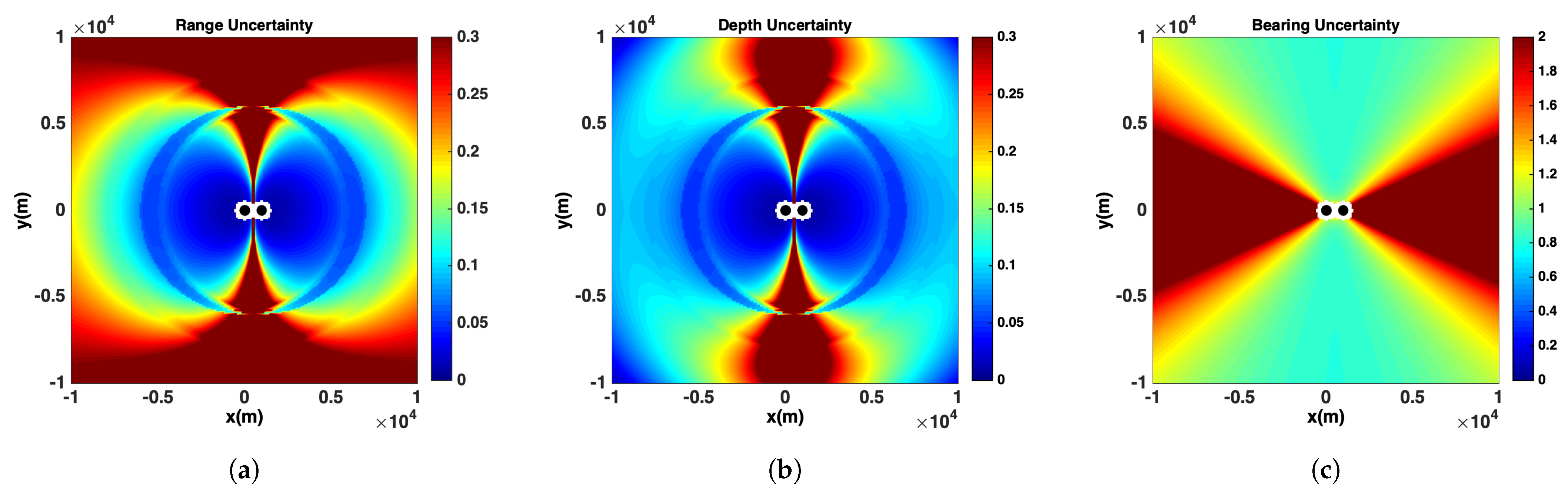
In order to compare between two- and three-hydrophone performance, Figure 11 presents the estimated uncertainty distributions for normalized range (left), normalized depth (center), and bearing (right) for a pair of hydrophones with the same separation (1 km) and depth (100 m), as in the previous examples, following the localization approach described in [16], extended to also exploit turning-point arrivals and corresponding TDOAs. In this connection, the caustics zone at ranges of about 6 km, associated with refracted turning-point arrivals, is observed in the uncertainty distributions for the normalized range and depth.

From a comparison of these results with the results that are shown in Figure 4 and Figure 9, the benefit of using three rather than two hydrophones becomes immediately apparent. With the three-hydrophone array, smaller uncertainties are obtained in general. While the two-hydrophone array has blind spots, areas of high uncertainty, such as the broadside direction for range and depth estimation and the endfire direction for bearing estimation, the considered three-hydrophone arrays demonstrate functional performance in all directions. Furthermore, the left-right ambiguity, characterizing hydrophone pairs, and linear arrays in general, is resolved with the addition of a third hydrophone, non-aligned with the other two.

3.2. 2D localization Uncertainty

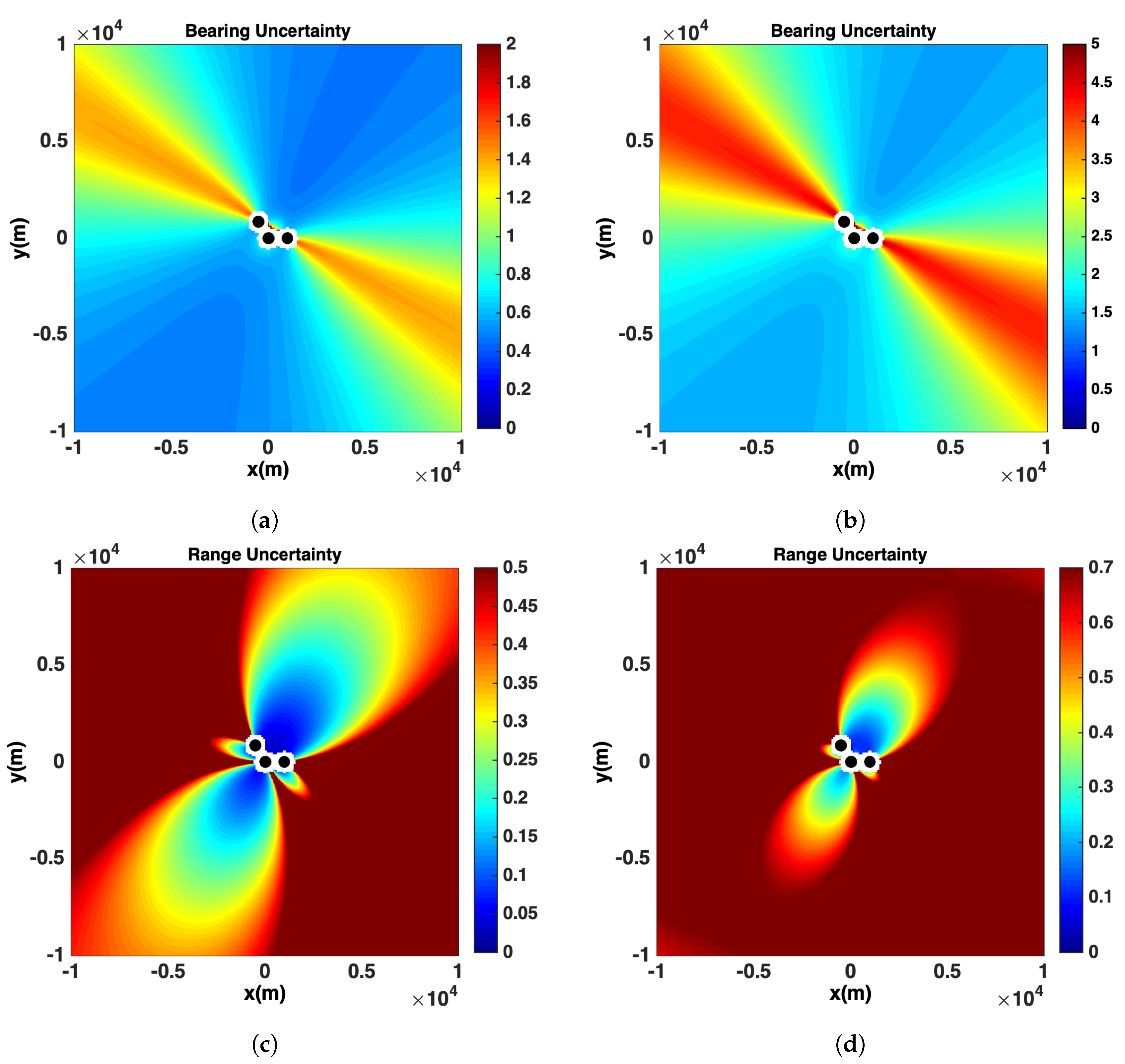
In this section, some uncertainty results for 2D localization, omitting the depth dimension and relying on direct arrivals [6], are presented. Figure 12 shows the estimated uncertainty distributions for source bearing (top) and relative range (bottom) for the obtuse array geometry and for different values in the uncertainty of the hydrophone location in the horizontal, 10 m RMS (left) and 30 m RMS (right), respectively. The same RMS error for TDOAs between direct arrivals as before has been used ($\delta {\tau }_{21,\mathrm{RMS}}=\delta {\tau }_{31,\mathrm{RMS}}=0.1$ ms). The bearing uncertainty distribution in the upper left panel is almost identical with the corresponding distribution from 3D localization (Figure 9a). This is a confirmation that, for the bearing estimation, the TDOAs between direct arrivals are sufficient [9]. The top right panel exhibits a deterioration in bearing estimation accuracy with hydrophone location uncertainty in the horizontal (note the difference in the color scales), and the bearing estimation in 3D localization (not shown) is affected in a similar way. This points to the importance of the hydrophone horizontal positioning accuracy for bearing estimation.

The bottom panels presented in Figure 12 show the uncertainties in normalized ranges. The uncertainties in Figure 12c are much larger than the ones that are shown in Figure 4a (note the difference in the color scales), even though a relatively small horizontal receiver location uncertainty is used (10 m RMS). On the other hand, the result shown in Figure 4a is independent of the uncertainty in the hydrophone location in the horizontal. In Figure 12d, the range estimation uncertainties are much larger due to the larger uncertainty in receiver locations in the horizontal (30 m RMS). The range/depth estimation in the 3D localization approach is not affected at all by this change. The uncertainty patterns shown in Figure 12c,d are similar to the 2D localization error results presented in [6], where larger uncertainties (50 m RMS) for the horizontal receiver locations are assumed.

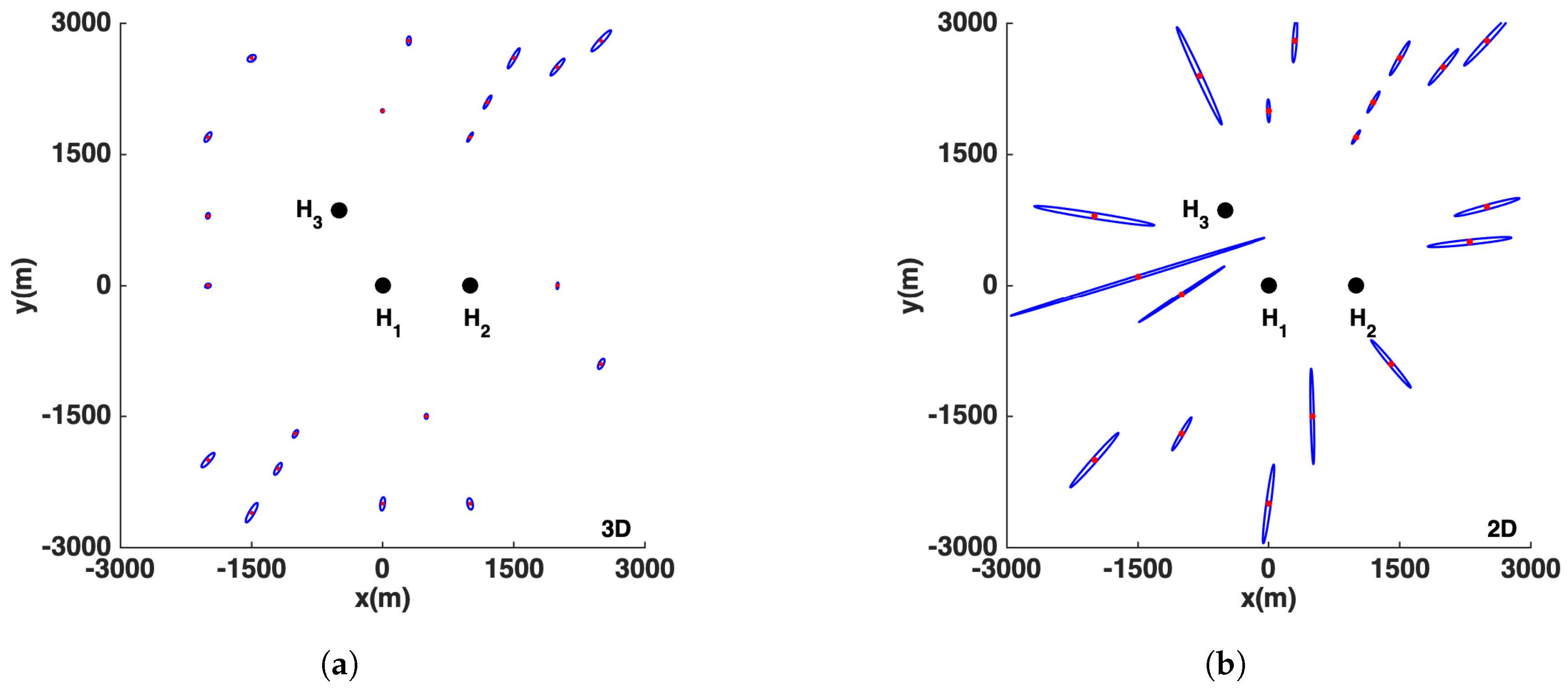
Figure 13 presents the RMS horizontal localization uncertainty ellipses resulting from the 3D and the 2D localization approaches for different source locations around the obtuse hydrophone array. For both approaches, an uncertainty of 10 m RMS is assumed for the receiver locations in the horizontal. While the bearing uncertainties from the two approaches are comparable, in agreement with the above remarks, the range uncertainties are very different in both magnitude and behavior. The range estimation uncertainties in 3D localization are larger close to the broadside and decrease towards the endfire of H${}_2$ and H${}_3$, the hydrophone pair with the largest separation. The 2D localization, on the other hand, results in much larger range uncertainties in general, which also follow the more complicated pattern of Figure 12c. This is because, in 2D localization, range estimation is obtained through the intersection of different bearings; in this connection the range uncertainties are smaller at the broadside of H${}_2$ and H${}_3$, still much larger than their 3D localization counterparts, simply because bearing estimation is subject to smaller uncertainties at the broadside. On the basis of these results, 2D localization is useful for bearing estimation, but quite questionable for range estimation. On the other hand, the exploitation of surface-reflected or turning-point arrivals results in smaller errors in range estimation and smaller dependence on receiver location accuracy.

4. Discussion

The proposed Bayesian localization approach aims at extending two-hydrophone source localization in a way that retains its advantages and eliminates its drawbacks, with the minimum possible addition, that of a third hydrophone, not in line with the other two. The present approach can be extended to an arbitrary number of hydrophones; nevertheless, the emphasis here is on keeping the array size small.

The environmental conditions are assumed range independent, being characterized by a single sound-speed profile measured close to the time of the localization; for ranges up to 10 km and in areas away from ocean fronts, the range dependence of the medium is expected to be of limited importance. The sound speed mode is introduced in order to account for small deviations from the measured sound-speed profile, e.g., due to warming or cooling in the near-surface layer, in the estimation of localization uncertainty. Thus, the sound-speed profile accounts for the gross refraction effects on localization, whereas the sound-speed mode serves the quantification of uncertainty.

Different array geometries were considered in order to study their effect on the uncertainty distributions. The optimal configuration in each case depends on deployment constraints and set goals. For example, for open-ocean deployments, the equilateral triangle, providing a nearly uniform coverage in the azimuth, would be in general preferable. On the other hand, for near-shore deployments where the emphasis is on covering a broad offshore sector, the obtuse geometry could provide acceptable uncertainties over a wider area.

The array geometries and dimensions that are considered in this work are associated with the design of a moored deep-water large-aperture acoustic observatory for sperm whales planned to be deployed in summer 2021 south of the island of Crete in the Eastern Mediterranean Sea, in the framework of the SAvEWhales project. Three hydrophones, each one suspended from a different surface platform, are planned to form a large-aperture array with separations of about 1 km. This is expected to result in small localization errors, while, at the same time, it will pose significant challenges that are related to arrival association [11,19,39] across the different hydrophones. The association problem will be addressed using a pattern cross-correlation approach that has been developed and will be presented in a future publication, together with experimental results. The synchronization between the hydrophones will be obtained by exploiting PPS (pulse per second) signals–periodic box-shaped pulses of duration 0.1 s and period 1 s–emitted from GPS satellites [18,37]. A thermistor chain is planned to be suspended from the central acoustic station, which will periodically measure the temperature profile in the upper water layer, in order to account for the environmental variability [40].

Regular sperm whale clicks have ICIs (inter-click intervals) that range between 0.5 and 2 s [41]. In order to cope with such repetition rates and possibly also with multiple vocalizations, the localization codes have been implemented in C-language resulting in short execution times, typically less than 0.03 s per 3D localization on a standard PC and, thus, enabling the development of a real-time monitoring system.

5. Conclusions

In this work an enhanced three-hydrophone 3D localization method addressing the pitfalls of two-hydrophone localization was presented. The addition of a third hydrophone, not aligned with the other two, removes the left-right ambiguity and lowers the range/ depth and bearing estimation uncertainties for sources at the broadside and the endfire of the array respectively, also offering useful fallback options, e.g., in the case of failure of one hydrophone.

Refraction is taken into account and turning-point arrivals are exploited, in addition to surface-reflected arrivals, enabling localization at longer ranges, which, however, may be influenced by the formation of caustics. Furthermore, significant differences in the uncertainty behavior of estimated source range and depth have been observed, caused by refraction and the induced nonlinearity of the isochrones at longer ranges.

The non-linearity of the model relations is treated through linearization and iterative inversions. The initialization affects the inversion results in the early iteration steps, as expected, nevertheless, the final estimates, after convergence, are independent of the initial guess.

The analytic uncertainty distributions for different array geometries are compared against the two-hydrophone array performance and against the empirical distributions that result from full, non-linear inversions, showing that the adopted local linearization scheme is a good approximation. Finally, the horizontal localization results are compared against 2D localization based on direct arrivals only.

References

- Bahr, A.; Leonard, J.J.; Fallon, M.F. Cooperative Localization for Autonomous Underwater Vehicles. Int. J. Robot. Res. 2009, 28, 714–728. [Google Scholar] [CrossRef]
- Kelland, N.C. Deep-Water Black Box Retrieval. Hydro International. 2009. Available online: Https://www.hydro-international.com/content/article/deep-water-black-box-retrieval (accessed on 1 September 2020).
- Hastie, G.D.; Wu, G.; Moss, S.; Jepp, P.; MacAulay, J.; Lee, A.; Sparling, C.E.; Evers, C.; Gillespie, D. Automated detection and tracking of marine mammals: A novel sonar tool for monitoring effects of marine industry. Aquat. Conserv. Mar. Freshw. Ecosyst. 2019, 29, 119–130. [Google Scholar] [CrossRef] [Green Version]
- Hildebrand, J.A.; Frasier, K.E.; Baumann-Pickering, S.; Wiggins, S.M.; Merkens, K.P.; Garrison, L.P.; Soldevilla, M.S.; McDonald, M.A. Assessing Seasonality and Density From Passive Acoustic Monitoring of Signals Presumed to be From Pygmy and Dwarf Sperm Whales in the Gulf of Mexico. Front. Mar. Sci. 2019, 6, 66. [Google Scholar] [CrossRef] [Green Version]
- Delikaris-Manias, S.; McCormack, L.; Huhtakallio, I.; Pulkki, V. Real-Time Underwater Spatial Audio: A Feasibility Study. In Proceedings of the the 144th Audio Engineering Society Convention, Milan, Italy, 23–26 May 2018. [Google Scholar]
- Wahlberg, M.; Møhl, B.; Teglberg, M.P. Estimating source position accuracy of a large-aperture hydrophone array for bioacoustics. J. Acoust. Soc. Am. 2001, 109, 397–406. [Google Scholar] [CrossRef] [Green Version]
- Nosal, E.; Neil Frazer, L. Track of a sperm whale from delays between direct and surface-reflected clicks. Appl. Acoust. 2006, 67, 1187–1201. [Google Scholar] [CrossRef]
- Rideout, B.P.; Dosso, S.E.; Hannay, D.E. Underwater passive acoustic localization of Pacific walruses in the northeastern Chukchi Sea. J. Acoust. Soc. Am. 2013, 134, 2534–2545. [Google Scholar] [CrossRef]
- Watkins, W.A.; Schevill, W.E. Sound source location by arrival-times on a non-rigid three-dimensional hydrophone array. Deep Sea Res. Oceanogr. Abstr. 1972, 19, 691–706. [Google Scholar] [CrossRef]
- Skarsoulis, E.K.; Frantzis, A.; Kalogerakis, M. Passive localization of pulsed sound sources with a 2-hydrophone array. In Proceedings of the Seventh European Conference on Underwater Acoustics (ECUA), Delft, The Netherlands, 5–8 July 2004. [Google Scholar]
- Thode, A. Tracking sperm whale (Physeter macrocephalus) dive profiles using a towed passive acoustic array. J. Acoust. Soc. Am. 2004, 116, 245–253. [Google Scholar] [CrossRef] [PubMed] [Green Version]
- Barlow, J.; Griffiths, E.T. Precision and bias in estimating detection distances for beaked whale echolocation clicks using a two-element vertical hydrophone array. J. Acoust. Soc. Am. 2017, 141, 4388–4397. [Google Scholar] [CrossRef]
- Skarsoulis, E.K.; Kalogerakis, M.A. Ray-theoretic localization of an impulsive source in a stratified ocean using two hydrophones. J. Acoust. Soc. Am. 2005, 118, 2934–2943. [Google Scholar] [CrossRef]
- Thode, A. Three-dimensional passive acoustic tracking of sperm whales (Physeter macrocephalus) in ray-refracting environments. J. Acoust. Soc. Am. 2005, 118, 3575–3584. [Google Scholar] [CrossRef]
- Skarsoulis, E.K.; Kalogerakis, M.A. Two-hydrophone localization of a click source in the presence of refraction. Appl. Acoust. 2006, 67, 1202–1212. [Google Scholar] [CrossRef]
- Skarsoulis, E.K.; Dosso, S.E. Linearized two-hydrophone localization of a pulsed acoustic source in the presence of refraction: Theory and simulations. J. Acoust. Soc. Am. 2015, 138, 2221–2234. [Google Scholar] [CrossRef] [PubMed]
- Skarsoulis, E.K.; Piperakis, G.; Kalogerakis, M.; Orfanakis, E.; Papadakis, P.; Dosso, S.E.; Frantzis, A. Underwater acoustic pulsed source localization with a pair of hydrophones. Remote Sens. 2018, 10, 883. [Google Scholar] [CrossRef] [Green Version]
- Miller, B.; Dawson, S.; Vennell, R. Underwater behavior of sperm whales off Kaikoura, New Zealand, as revealed by a three-dimensional hydrophone array. J. Acoust. Soc. Am. 2013, 134, 2690–2700. [Google Scholar] [CrossRef] [PubMed] [Green Version]
- Morrissey, R.; Ward, J.; DiMarzio, N.; Jarvis, S.; Moretti, D.J. Passive acoustic detection and localization of sperm whales (Physeter macrocephalus) in the tongue of the ocean. Appl. Acoust. 2006, 67, 1091–1105. [Google Scholar] [CrossRef]
- Miller, B.; Dawson, S. A large-aperture low-cost hydrophone array for tracking whales from small boats. J. Acoust. Soc. Am. 2009, 126, 2248–2256. [Google Scholar] [CrossRef] [Green Version]
- Baggenstoss, P.M. An algorithm for the localization of multiple interfering sperm whales using multi-sensor time difference of arrival. J. Acoust. Soc. Am. 2011, 130, 102–112. [Google Scholar] [CrossRef] [Green Version]
- Brunoldi, M.; Bozzini, G.; Casale, A.; Corvisiero, P.; Grosso, D.; Magnoli, N.; Alessi, J.; Bianchi, C.N.; Mandich, A.; Morri, C.; et al. A Permanent Automated Real-Time Passive Acoustic Monitoring System for Bottlenose Dolphin Conservation in the Mediterranean Sea. PLoS ONE 2016, 11, 1–35. [Google Scholar] [CrossRef]
- Leaper, R.; Chappell, O.; Gordon, J.C.D. The development of practical techniques for surveying sperm whale populations acoustically. In Report of the International Whaling Commission 42; The Red House: Cambridge, UK, 1992; pp. 549–560. [Google Scholar]
- Urazghildiiev, I.R.; Hannay, D. Maximum likelihood estimators and Cramér–Rao bound for estimating azimuth and elevation angles using compact arrays. J. Acoust. Soc. Am. 2017, 141, 2548–2555. [Google Scholar] [CrossRef]
- Urazghildiiev, I.R.; Hannay, D.E. Localizing Sources Using a Network of Asynchronous Compact Arrays. IEEE J. Ocean. Eng. 2020, 45, 1091–1098. [Google Scholar] [CrossRef]
- Sanguineti, M.; Alessi, J.; Brunoldi, M.; Cannarile, G.; Cavalleri, O.; Cerruti, R.; Falzoi, N.; Gaberscek, F.; Gili, C.; Gnone, G.; et al. An automated passive acoustic monitoring system for real time sperm whale (Physeter macrocephalus) threat prevention in the Mediterranean Sea. Appl. Acoust. 2021, 172, 107650. [Google Scholar] [CrossRef]
- Barlow, J.; Griffiths, E.T.; Klinck, H.; Harris, D.V. Diving behavior of Cuvier’s beaked whales inferred from three-dimensional acoustic localization and tracking using a nested array of drifting hydrophone recorders. J. Acoust. Soc. Am. 2018, 144, 2030–2041. [Google Scholar] [CrossRef] [PubMed]
- Barlow, J.; Fregosi, S.; Thomas, L.; Harris, D.; Griffiths, E.T. Acoustic detection range and population density of Cuvier’s beaked whales estimated from near-surface hydrophones. J. Acoust. Soc. Am. 2021, 149, 111–125. [Google Scholar] [CrossRef] [PubMed]
- Gassmann, M.; Henderson, E.; Wiggins, S.M.; Roch, M.A.; Hildebrand, J.A. Offshore killer whale tracking using multiple hydrophone arrays. J. Acoust. Soc. Am. 2013, 134, 3513–3521. [Google Scholar] [CrossRef]
- Gassmann, M.; Wiggins, S.M.; Hildebrand, J.A. Three-dimensional tracking of Cuvier’s beaked whales’ echolocation sounds using nested hydrophone arrays. J. Acoust. Soc. Am. 2015, 138, 2483–2494. [Google Scholar] [CrossRef] [Green Version]
- Dosso, S.E.; Ebbeson, G.R. Array element localization accuracy and survey design. Can. Acoust. 2006, 34, 3–13. [Google Scholar]
- Thomson, D.; Dosso, S. AUV localization in an underwater acoustic positioning system. In Proceedings of the 2013 MTS/IEEE OCEANS—Bergen, Bergen, Norway, 10–14 June 2013; pp. 1–6. [Google Scholar]
- Warner, G.A.; Dosso, S.E.; Hannay, D.E. Bowhead whale localization using time-difference-of-arrival data from asynchronous recorders. J. Acoust. Soc. Am. 2017, 141, 1921–1935. [Google Scholar] [CrossRef]
- Apostol, T.M. Calculus, Vol. 2: Multi-Variable Calculus and Linear Algebra with Applications to Differential Equations and Probability, 2nd ed.; J. Wiley: Hoboken, NJ, USA, 1975; Volume 2. [Google Scholar]
- Berger, J.O. Statistical Decision Theory and Bayesian Analysis; Springer Series in Statistics; Springer: New York, NY, USA, 1985. [Google Scholar]
- Tarantola, A. Inverse Problem Theory, 1st ed.; Elsevier: New York, NY, USA, 1987; Volume 2. [Google Scholar]
- Niu, X.; Yan, K.; Zhang, T.; Zhang, Q.; Zhang, H.; Liu, J. Quality evaluation of the pulse per second (PPS) signals from commercial GNSS receivers. GPS Solut. 2015, 19, 141–150. [Google Scholar] [CrossRef]
- Godin, O.A.; Fuks, I.M. Travel-time statistics for signals scattered at a rough surface. Waves Random Media 2003, 13, 205–221. [Google Scholar] [CrossRef]
- Giraudet, P.; Glotin, H. Real-time 3D tracking of whales by echo-robust precise TDOA estimates with a widely-spaced hydrophone array. Appl. Acoust. 2006, 67, 1106–1117. [Google Scholar] [CrossRef]
- Taniguchi, N.; Sakuno, Y.; Mutsuda, H.; Arai, M. Revisiting a coastal acoustic tomography experiment in Hiroshima Bay: Temporal variations in path-averaged currents and its relation to wind. Appl. Ocean Res. 2020, 102, 102303. [Google Scholar] [CrossRef]
- Goold, J.C.; Jones, S.E. Time and frequency domain characteristics of sperm whale clicks. J. Acoust. Soc. Am. 1995, 98, 1279–1291. [Google Scholar] [CrossRef] [PubMed]
Figure 1.
Direct and surface-reflected paths from a source to a three-hydrophone array and the corresponding travel times.
Figure 2.
Sound speed profile (left panel) and vertical sound-speed mode (right panel).
Figure 3.
The three-hydrophone geometries considered: (a) obtuse triangle, (b) right triangle, (c) equilateral triangle. and (d) two-hydrophone array.
Figure 4.
Posterior RMS uncertainty distributions for normalized source range (a–c) and depth (d–f) as a function of source position in the horizontal (source depth 800 m) for the three array geometries considered. The marked points, A, B, and, C in the leftmost panels denote source locations for Monte Carlo simulations.
Figure 5.
Surface-reflected (cyan) and turning-point rays (grey) emanating from a receiver at 100 m depth, after reflection/turning point. Black lines: Isochrones corresponding to 5 (shallowest), 10, 15, and 20 ms (deepest).
Figure 6.
Normalized histograms of source range (a–c) and depth (d) deviations for source location A (Figure 4a,d) from 5000 non-linear inversions of randomly perturbed data sets. The red solid curves are the corresponding analytic posterior PDFs.
Figure 7.
Normalized histograms of source range (a–c) and depth (d) deviations for source location B (Figure 4a,d) from 5000 non-linear inversions of randomly perturbed data sets. The red solid curves are the corresponding analytic posterior PDFs.
Figure 8.
Normalized histograms of source range (a–c) and depth (d) deviations for source location C (Figure 4a,d) from 5000 non-linear inversions of randomly perturbed data sets. The red solid curves are the corresponding analytic posterior PDFs.
Figure 9.
Posterior RMS uncertainty distributions for bearing estimation from 3D localization as a function of source position in the horizontal for the three array geometries considered, (a) obtuse, (b) right, and (c) equilateral.
Figure 10.
Examples of iterative localization in the xy-plane for the obtuse array geometry, for source locations A, B, and C defined in Figure 4, leftmost (a,d), middle (b,e), and rightmost (c,f) panels, respectively. A circle denotes the true source location, a cross the final estimation result, the ×’s denote intermediate estimates, and a diamond marks the initial guess. The ellipses represent the localization uncertainties corresponding to one standard deviation. Full/detailed views are presented in the upper/lower panels, respectively.
Figure 11.
Posterior RMS uncertainty distributions for normalized source range (a), depth (b), and bearing (c) from two-hydrophone localization as a function of the source position in the horizontal. The source depth is 800 m.
Figure 12.
Posterior RMS uncertainty distributions for source bearing (a,b) and relative source range (c,d) from 2D localization as a function of source position in the horizontal for the obtuse array geometry assuming different RMS uncertainties for the hydrophone locations in the horizontal: (a,c) 10 m. (b,d) 30 m.
Figure 13.
RMS ellipses demonstrating the posterior localization uncertainties corresponding to one standard deviation for various source locations around the obtuse array. (a) 3D localization. (b) 2D localization.
Publisher’s Note: MDPI stays neutral with regard to jurisdictional claims in published maps and institutional affiliations. |
© 2021 by the authors. Licensee MDPI, Basel, Switzerland. This article is an open access article distributed under the terms and conditions of the Creative Commons Attribution (CC BY) license (https://creativecommons.org/licenses/by/4.0/).
Share and Cite
MDPI and ACS Style
Pavlidi, D.; Skarsoulis, E.K. Enhanced Pulsed-Source Localization with 3 Hydrophones: Uncertainty Estimates. Remote Sens. 2021, 13, 1817. https://0-doi-org.brum.beds.ac.uk/10.3390/rs13091817
AMA Style
Pavlidi D, Skarsoulis EK. Enhanced Pulsed-Source Localization with 3 Hydrophones: Uncertainty Estimates. Remote Sensing. 2021; 13(9):1817. https://0-doi-org.brum.beds.ac.uk/10.3390/rs13091817
Chicago/Turabian StylePavlidi, Despoina, and Emmanuel K. Skarsoulis. 2021. "Enhanced Pulsed-Source Localization with 3 Hydrophones: Uncertainty Estimates" Remote Sensing 13, no. 9: 1817. https://0-doi-org.brum.beds.ac.uk/10.3390/rs13091817
Note that from the first issue of 2016, this journal uses article numbers instead of page numbers. See further details here.