
Investigating the Response of Temperature and Salinity in the Agulhas Current Region to ENSO Events


1
Naval Research Laboratory, Stennis Space Center, Mississippi, Hancock County, MS 39529, USA
2
School of the Earth, Ocean, and Environment, University of South Carolina, Columbia, SC 29208, USA
*
Author to whom correspondence should be addressed.
Remote Sens. 2021, 13(9), 1829; https://0-doi-org.brum.beds.ac.uk/10.3390/rs13091829
Submission received: 21 March 2021
/
Revised: 22 April 2021
/
Accepted: 5 May 2021
/
Published: 7 May 2021
(This article belongs to the Special Issue Moving Forward on Remote Sensing of Sea Surface Salinity)
Abstract
:The Agulhas Current is a critical component of global ocean circulation and has been observed to respond to El Niño Southern Oscillation (ENSO) events via its temperature and salinity signatures. In this research, we use sea surface salinity (SSS) from the National Aeronautics and Space Administration’s (NASA) Soil Moisture Active Passive (SMAP) satellite, sea surface temperature (SST) observations from the Canadian Meteorological Centre (CMC), sea surface height (SSH) anomalies from altimetry, and the Oceanic Niño Index to study the SMAP satellite time period of April 2015 through March 2020 (to observe full years of study). We see warming and high salinities after El Niño, cooling and fresher surface waters after La Niña, and a stronger temperature response than that of salinity. About one year after the 2015 El Niño, there is a warming of the entire region except at the Antarctic Circumpolar Current. About two years after the event, there is an increase in salinity along the eastern coast of Africa and in the Agulhas Current region. About two years after the 2016 and 2018 La Niñas, there is a cooling south of Madagascar and in the Agulhas Current. There are no major changes in salinity seen in the Agulhas Current, but there is a highly saline mass of water west of the Indonesian Throughflow about two years after the La Niña events. Wavelet coherence analysis finds that SSS and ENSO are most strongly correlated a year after the 2015 El Niño and two years after the 2016 La Niña.
1. Introduction
The variability of currents that are a part of the global conveyor belt, such as the Agulhas Current, can have major impacts on global climate. The Agulhas Current is a western boundary current that flows off the eastern coast of South Africa. It originates south of the Mozambique Channel and flows towards the southern tip of Africa where it retroflects back into the Indian Ocean. Generally, the retroflection is between 16° E and 20° E with a loop diameter of 340 km and it sheds rings into the Atlantic that are about 320 km in diameter [1]. The Agulhas Current does shed some of its water as rings, but most is retroflected along with water from the Southern Ocean [2]. The rings that the Agulhas Current sheds in the area of retroflection are some of the largest mesoscale eddies in the world which transfer water from the Indian Ocean into the Atlantic Ocean, creating the Agulhas Leakage [3]. This retroflection is the result of a net accumulation of anticyclonic relative vorticity [1]. The Agulhas Leakage and the Agulhas Return Current are how the Indian, Atlantic, and Southern Oceans are physically connected.
The Agulhas Leakage forms part of the Atlantic Meridional Overturning Circulation (AMOC). This circulation consists of about 14 Sv (1 Sv = 106 m3 s−1) of deep water flowing southward across the equator and the northward heat flux with a maximum value of 1 PW (1015 W) [4]. The Agulhas Leakage alters the AMOC by transporting the warmer and more saline waters of the Indian Ocean into the Atlantic [2,5,6]. Waters from the Indian, Atlantic, and Southern Oceans all meet and interact in such a leakage region. The transport of water from ocean to ocean with different salinity and temperature profiles means that the Agulhas Leakage has the potential to alter thermohaline properties in the Atlantic and therefore the AMOC [7], which is important because it affects climate and the ecosystem. Previous studies have indicated that the Agulhas Current strongly responds to teleconnections such as the El Niño Southern Oscillation (ENSO) which can change temperature, salinity, and sea surface height, among others.
The effect of an El Niño or La Niña can be seen with altimeters as sea surface height (SSH) anomalies locally increase due to El Niño and decrease due to La Niña in the western equatorial Pacific. The effects of ENSO have been shown to reach the Indian Ocean [8,9]. The ENSO-affected waters of the Indian Ocean then feed into the Agulhas Current. It is estimated that 11.5% of the variance in transport in the Agulhas Current can be attributed to ENSO [10].
Multiple studies have found that the effects of ENSO can be seen in the Agulhas Current approximately two years after each El Niño or La Niña [5,11]. The Agulhas Leakage sea surface temperature (SST) responds two years after El Niño as anomalously warm and two years after La Niña as anomalously cool [11]. In response to El Niño, the primary signal of sea surface salinity (SSS) was anomalously fresh, and then the secondary signal was anomalously saline. The primary response to La Niña was anomalously saline, and then waters became anomalously fresh [12].
The objective of this work is to determine how ENSO affects the temperature and salinity of the Agulhas Current and the Agulhas Leakage with a focus on salinity. This study will use Canadian Meteorological Centre (CMC) SST, Soil Moisture Active Passive (SMAP) SSS, and Copernicus Marine Environment Monitoring Service (CMEMS) SSH anomalies to explore the effect of ENSO on the Agulhas Current. Other studies used models and reanalyses, but this project is the first of its kind to use SMAP, the most recently launched SSS satellite. As this satellite is so new, it is important to evaluate how well it detects SSS in this region. The most recent El Niño in 2015 and La Niñas in 2016 and 2018 will be used as reference points because they occurred during the SMAP satellite era. By analyzing satellite data, we will be able to find the effects of ENSO on the Agulhas Current and leakage.
2. Data and Methods
2.1. Satellite Data
SSS data from the SMAP (Soil Moisture Active Passive) satellite, developed and processed by NASA’s Jet Propulsion Laboratory (JPL), were used in this paper. These data use a Level 3 8-day running mean for complete spatial coverage. We used the monthly average of version 4.3 which has a resolution of 0.25 degrees and an improved land bias correction algorithm [13]. It is important to evaluate how well SMAP detects SSS in this region due to its novelty and because its temporal period encompasses both El Niño and La Niña events. SMAP provides more detailed maps of SSS than previous products and ARGO buoys [14]. https://podaac.jpl.nasa.gov/announcements/2020-03-18_JPL_SMAP_SSS_CAP_Dataset_Release, accessed on 21 March 2021.
SST anomalies developed by the Group for High Resolution Sea Surface Temperature (GHRSST) were obtained from the Canadian Meteorological Centre (CMC). This dataset merges the SST from multiple radiometers and in situ observations. The spatial resolution of this dataset is 0.2 degrees and daily files are used. The CMC SST uses data from microwave instruments, and when compared to other SST datasets, especially that of Argo, it had the smallest mean standard deviation [15]. https://podaac.jpl.nasa.gov/dataset/CMC0.2deg-CMC-L4-GLOB-v2.0, accessed on 21 March 2021.
SSH anomalies processed by the Copernicus Marine Environment Monitoring Service (CMEMS) multimission data processing system, which processes data from all altimeter missions: Jason-3, Sentinel-3A, HY-2A, Saral/AltiKa, Cryosat-2, Jason-2, Jason-1, T/P, ENVISAT, GFO, and ERS1/2, were used. These data are provided by the Copernicus Marine Environment Monitoring Service (CMEMS). These data have a resolution of 0.25 degrees and daily files are used. As multiple satellite altimeters are processed, this improves the accuracy and spatial resolution of SSH anomaly changes [16]. (https://resources.marine.copernicus.eu/?option=com_csw&task=results&product_id=SEALEVEL_GLO_PHY_L4_REP_OBSERVATIONS_008_047&view=details, accessed on 21 March 2021).
2.2. Oceanic Niño Index
ENSO events in this study were determined by the Oceanic Niño Index (ONI) from the National Weather Service Climate Prediction Center. The ONI calculates the 3-month running mean of ERSST.v5 (Extended Reconstructed Sea Surface Temperature) SST anomalies in the Niño 3.4 region (5° N–5° S, 120°–170° W) based on centered 30-year base periods updated every 5 years. Warm and cold periods are based on a threshold of −0.5 degrees or 0.5 degrees. https://origin.cpc.ncep.noaa.gov/products/analysis_monitoring/ensostuff/ONI_v5.php, accessed on 21 March 2021.
2.3. In Situ Observations of Argo Temperature and Salinity
Subsurface temperature and salinity profile data were provided by Argo floats from the Asia-Pacific Data-Research Center (APRDC), University of Hawaii. These data are binned to 1 degree × 1 degree monthly means from January 2005 to April 2020. These data allow us to observe the water column of the region and not just the surface characteristics and have sufficient coverage in this region to be used in this work [17]. (http://apdrc.soest.hawaii.edu/datadoc/argo_iprc_gridded.php, accessed on 21 March 2021).
2.4. Bathymetry
We used bathymetric data from the General Bathymetric Chart of the Oceans 2020 grid (GEBCO_2020; GEBCO.net, accessed on 21 March 2021). This product has a horizontal resolution of 1/240° and is derived from a wide variety of observations, including single-beam and multibeam echo-sounders, lidar, seismic methods, satellite-derived gravity data, and Electronic Navigation Chart soundings.
2.5. Methods
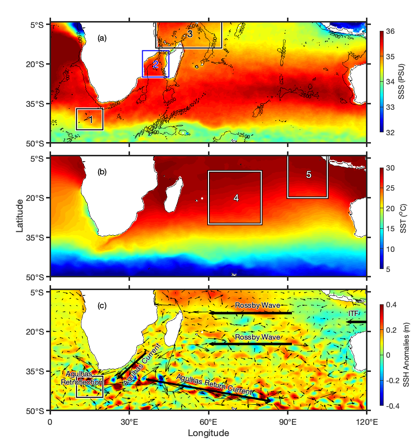
To observe the full pathways of ENSO signals across the Indian Ocean during the SMAP time period (beginning in April 2015), the area of study chosen is 0°–120° E and 5° S–55° S, which covers the full southern Indian Ocean as well as the full Agulhas Leakage and Agulhas Retroflection regions. The Agulhas Leakage in this paper is referenced primarily by the region enclosed by 37°–45° S and 10°–20° E (box 1 in Figure 1a), like in [12]. The western limit of this box is the Good Hope transect and the eastern limit is the point of retroflection [6,7,12]. The regions selected for the central Indian Ocean box (10°–30° S, 60°–80° E; box 4 in Figure 1b) and eastern Indian Ocean box (0°–20° S, 90°–105° E; box 5 in Figure 1b) for tracing the penetration and propagation of each temperature and salinity signal in our depth–time analysis were also intentionally selected. The eastern box is at a location that captures the origin of the ENSO signal [12] and its interaction with the Indonesian Throughflow region. The central box captures the propagating signal as it approaches the source currents of the Agulhas region immediately before the signal interacts with the East Madagascar Current retroflection [12]. The other boxes used in our correlation analysis were designed to follow the ENSO event signals through the Mozambique Channel and are portrayed in Figure 1a (boxes 2 and 3 in Figure 1a). Boxes 1–3 (Figure 1a) were selected based on the local topography and follow the pathway that the ENSO signal takes around Madagascar to the Agulhas Current region, and boxes 4 and 5 (Figure 1b) were selected based on their temperature and salinity profiles and capture the ENSO signal along westward-propagating Rossby waves in the Indian Ocean.
Monthly temperature and salinity anomalies were computed in reference to the monthly climatology of 2016–2020, where the monthly climatology was subtracted from each monthly mean. The years for the climatology were selected to include the full years of SMAP data, which are available beginning in April 2015. It is important to note that many figures in this manuscript reference particular seasons, especially the period of January through March. This is because ENSO events typically peak during this time of year (January–March) [8].
A Pearson product-moment correlation coefficient analysis was performed to find the lag between the peak of ENSO signals and box-averaged SST and SSS at the Agulhas Retroflection region following the methodology conducted by Paris et al. [12]. The peak in the ENSO signal was defined as the average ONI value during the peak (December–March) of defined El Niño or La Niña years. This was correlated with the 3-month running mean of box-averaged SST and SSS at monthly lag intervals from the corresponding El Niño or La Niña years.
Wavelet coherence analysis, which examines the relationship between two time series, was applied to determine the timing and magnitude of oscillations in this region [18]. Wave coherence is analogous to taking a correlation coefficient (r2) for two time series in the time–frequency space, as applied to a Morlet wavelet, and has the same scale of 0 to 1, with the value expressed describing the amount of variance explained [19].
3. Results
3.1. Surface Characteristics
Climatological SMAP SSS (Figure 1a), CMC SST (Figure 1b), and CMEMS SSH anomalies (Figure 1c) reveal large-scale ocean features in the region of interest that encompasses the southern Indian Ocean and Agulhas Current region. The subtropical gyre in the southern Indian Ocean is visible as a band of high salinities (>35 psu) and the low-salinity waters of the ITF. The mechanism by which ENSO signals propagate across the Indian Ocean is by Rossby waves at 8° S and 22.5° S [12]. The most clearly visible features in the average SST are the ACC and the retroflection point of the Agulhas Current (Figure 1b). In the SSH anomalies, the eddy train associated with the Agulhas Retroflection is clear at about 35° S across nearly the entire southern Indian Ocean (Figure 1c). Ocean currents and features relevant to this work are identified in Figure 1c.
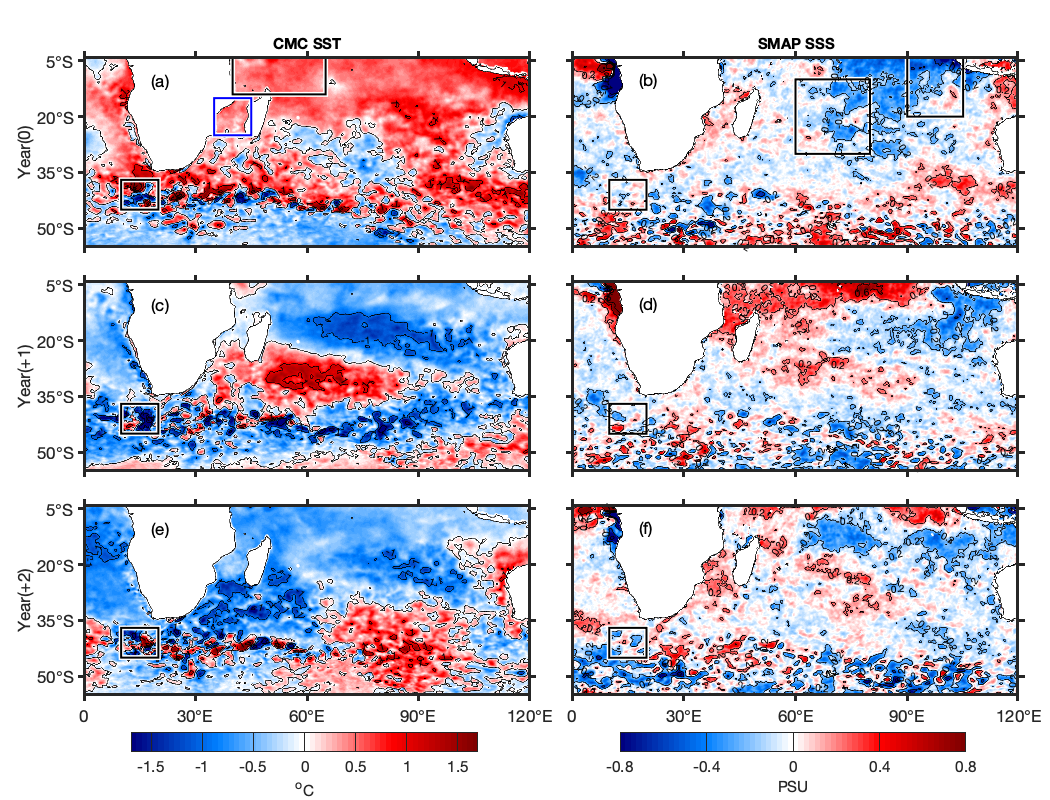
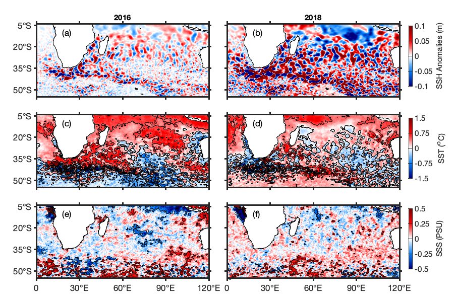
SST anomalies and SSS anomalies for the 2016 and 2018 La Niña events for those identified years, their respective successive year, and the two years following each event are, respectively, presented in Figure 2 and Figure 3 (Figure 2 is for 2016 and Figure 3 is for 2018). We compare the different years to see changes that can be attributed to La Niña and follow the evolution of the oceanic response. Much of the southern Indian Ocean experiences a shift from anomalously warm in Figure 2a to anomalously cool in Figure 2c, with the exception of the warm water mass at 20°–35° S and 40°–80° E. Cool waters enter the region from the western Pacific through the Indonesian Throughflow (ITF) [20] in Figure 2c and then flow into the Agulhas Current in Figure 2e. There is a less spatially uniform change in SSS when compared to that of SST for the overall domain in Figure 2. A year after Figure 2b, in Figure 2d, there is a mass of anomalously fresh water in the upper right representing the ITF. In Figure 2f, the anomalously fresh water mass appears to weaken as it propagates westward and comes in contact with the highly saline Arabian Sea waters [21] and only propagates to about 60° E, while the temperature signal at this same time fully extends across the southern Indian Ocean and towards the northern tip of Madagascar.
Regarding the 2018 La Niña, there is, again, a basin-scale SST anomaly reversal (in Figure 2a,c from warm to cool, and in Figure 3a,c from cool to warm), with a unique temperature signal at 20°–35° S and 40°–80° E and a meridionally oriented temperature dipole two years after the event’s peak (Figure 2e and Figure 3e). SMAP SSS again primarily identifies the anomalous ITF flow as the primary mechanism for the ENSO SSS signal propagation across the Indian Ocean, which is expected and is well captured by the SMAP satellite. It is important to note that the 2016 La Niña event is slightly stronger than that of 2018, according to the ONI, hence the ITF SSS variability (Figure 2f and Figure 3f). We will elaborate further on this differing surface response later in this section.
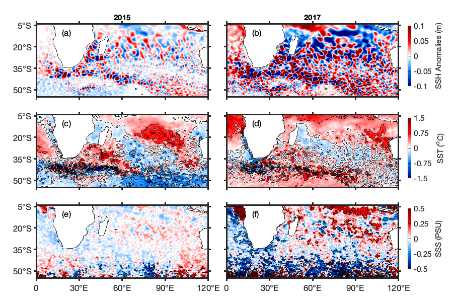
SST anomalies and SSS anomalies of the 2015 El Niño event a year after and two years after the event itself are presented in Figure 4. The 2015 El Niño is not included because there is no SMAP salinity data for 2015 until April, which is after the January–March period of peak event intensity. Overall, the temperature shifts from anomalously warm in Figure 4a to anomalously cool in Figure 4c. Warm water circulates in the Agulhas Current during this time and is no longer present the subsequent year. We trace the warm water signal in Figure 4a along westward-propagating Rossby waves later in this manuscript and confirm that its location and timing is consistent with heavy rainfall associated with the 2015 El Niño event [20]. There is a region of anomalously cooler waters that experiences warming and then cooling again as per the progression in Figure 4a through Figure 4c southeast of Madagascar. The difference in the region southeast of Madagascar’s temperature compared to the rest of the region is consistent among other figures (Figure 2, Figure 3 and Figure 5). This is the point at which the Agulhas Return Current (ARC) recirculates and initiates mixing and advection of the Indian, Atlantic, and Southern Ocean waters into the ARC [2].
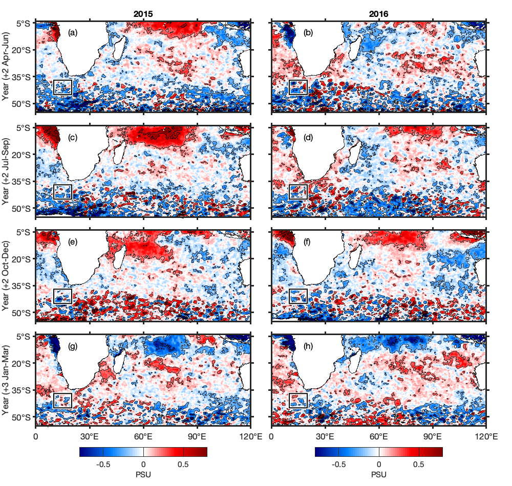
The composite mean of SSS anomalies for two years after the 2016 and 2018 La Niña events and the 2015 El Niño event in April–June (Figure 5a,b), July–September (Figure 5c,d), October–December (Figure 5e,f), and three years after in January–March (Figure 5g,h) traces the SSS signal westward across the Indian Ocean and into the Agulhas Current region. Figure 5a,c have a mass of anomalously saline water in the northwestern part of the region displayed which may be attributed to the previous El Niño event in 2015, as seen in Figure 5d. Fresher waters enter the region in response to La Niña events (Figure 5a,c,e,g) [12] via the ITF, travel westward (Figure 5e) into the inflow point of the Mozambique Channel (Figure 5g), driven by the South Equatorial Current, and feed into the Agulhas Current. In the El Niño column (Figure 5b,d,f,h), there is a mass of anomalously saline water in Figure 5b–f. No timesteps reveal this mass entering the region from the western Pacific, so it is likely unrelated to ENSO events [20]. Three years after the El Niño event (Figure 5h), there is a large mass of anomalously saline water at about 5–25° S, 70–115° E that enters the northwestern part of the whole region from the ITF, as seen in Figure 1f. As there is anomalously saline water appearing from the Pacific one year after the El Niño (Figure 4a) and three years after (Figure 5h), it cannot be comfortably assumed that this increase in salinity is directly related to ENSO. Other factors can change the SSS of the Indian Ocean such as the Indian Ocean Dipole (IOD) [22].
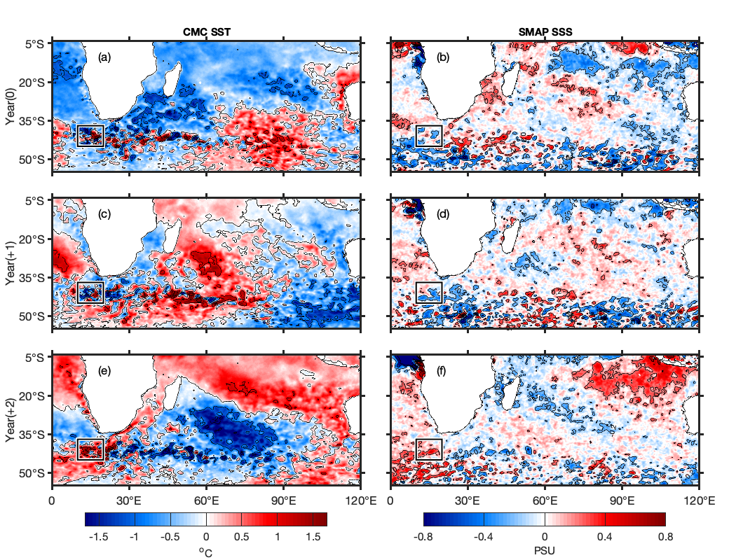
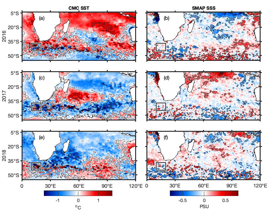
SST anomalies and SSS anomalies for the 2016 La Niña event (Figure 6) for that identified year, its successive year, and two years following the event identify a general shift from anomalously warm to anomalously cool waters over the entire domain from Figure 6a–c, with the exception of the region southeast of Madagascar, which experiences an opposite response. The cause of the anomalously warm waters in 2016 may be because of the 2015 El Niño event effects appearing a year later, as seen in Figure 4a. The region becomes anomalously cool in Figure 4e when the cool water moves westward into the Mozambique Channel and into the Agulhas Current. There is minor freshening from Figure 6d–f in the entirety of the region and anomalously cold and less saline water in the ITF region in Figure 6d that expands in Figure 6f, signifying increased ITF fresh water from the effects of La Niña. The region does become more saline from Figure 6b to Figure 6d, perhaps due to the effects of the 2015 El Niño two years later, as revealed in Figure 4d.
The composite mean of SSS and SST of the 2016 La Niña event minus the composite mean of SSS and SST of the 2018 La Niña event for January–March is presented in Figure 7. Both La Niña events are considered weak, but 2018 is slightly stronger [23]. During year zero (Figure 7a), there is a meridional SSTA dipole with warmer waters north of 35° S and cooler waters south of 35° S (with the exception of the West Australian Current upwelling). This pattern is true for the entire selected domain. This could be attributed to El Niño conditions at this point from the 2015 El Niño [22]. After one year (Figure 7c), this pattern of warmer waters is constrained from about 32° S to 35° S, and there is a similar band of cooler waters stretching along 35° S to 40° S. These are the remnants of warm waters that pass southward through the Mozambique Channel and then eastward due to the Agulhas Retroflection. After two years, the anomalously warm temperatures intensify within a concentrated region (60° E–90° E, 20° S–60° S). At this point (Figure 7e), the meridional temperature anomaly dipole has completely flipped, with cooler waters to the north and warmer waters to the south (relative to 30° S) once the signal has had ample time to propagate.
It is interesting to note the clear difference in timing between the temperature and salinity of these two La Niña events. Not only does the SMAP salinity measure a slower reaction timing than that of temperature but we also see a slightly different pathway between the signal of SMAP SSS and that of CMC SST. While the initial state is again dipolar (Figure 7b), the saline response to La Niña events along westward-propagating Rossby waves is not clear until one year later (Figure 7d), and by the time the signal has reached the Agulhas Current region (Figure 7f), there is a clear bifurcation of the southward-flowing salinity signal, split by Madagascar. One branch flows through the Mozambique Channel, while the other follows the circulation pattern of the Indian Ocean Gyre (Figure 7f). SMAP SSS not only clearly measured the timing of the SSS response with respect to the Agulhas Current region but also illustrated signal pathways not seen in SST.
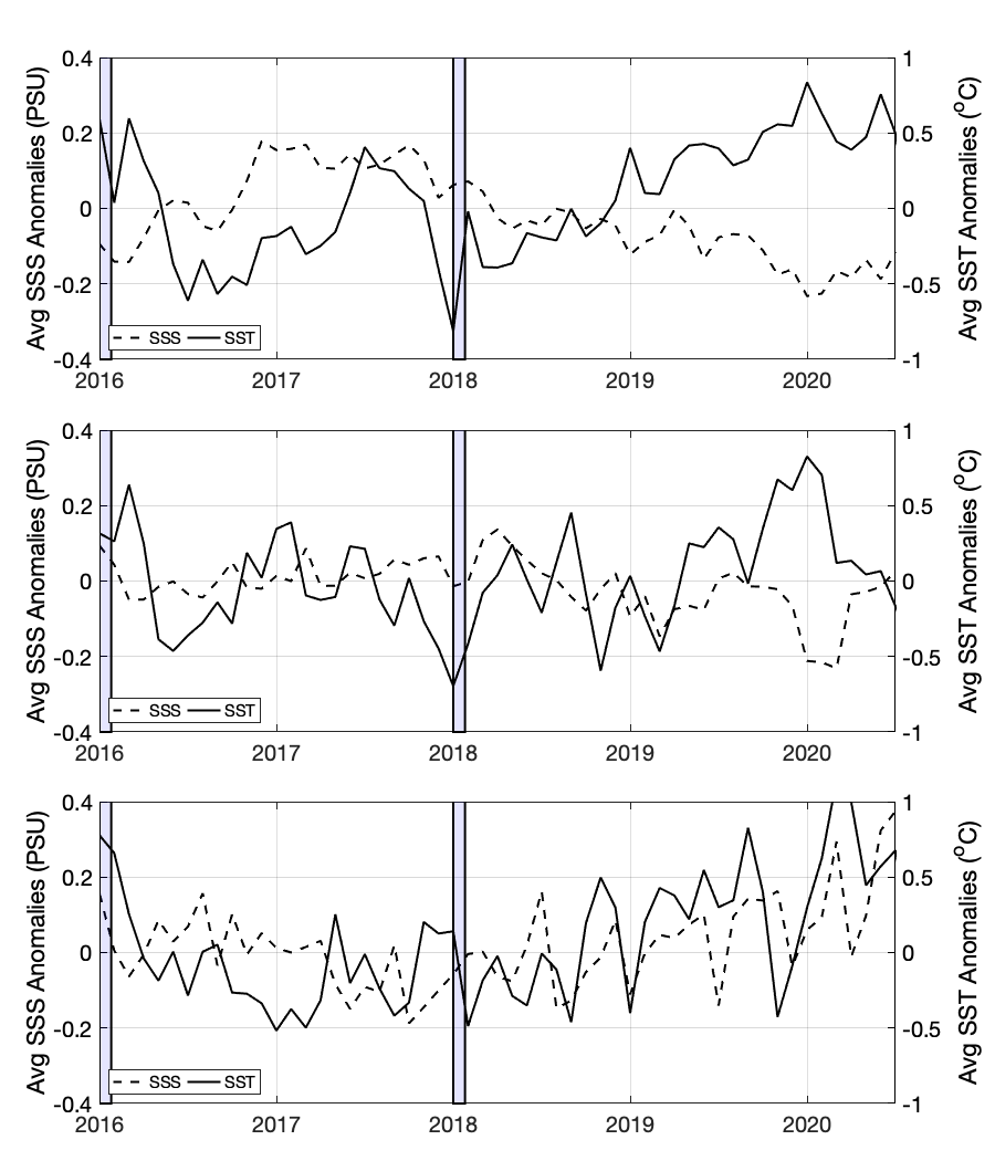
Three time series of SST and SSS from 2016 to 2020 represent a region north of Madagascar (Figure 8, top panel, box 3 in Figure 1), a region between Madagascar and the coast of Africa in the Mozambique Channel (Figure 8, middle panel, box 2 in Figure 1), and the Agulhas Leakage region (Figure 8, bottom panel, box 1 in Figure 1). These three regions compose the path that water from the Rossby wave outflow point travels before entering the Agulhas Current. The water in the Agulhas Current originates north of Madagascar (box 3 in Figure 1), enters the Mozambique Channel (box 2 in Figure 1), and then flows into the Agulhas Current (box 1 in Figure 1). Figure 8 provides a temporal visual of the anomalies represented in the previous figures. In the top panel, water is anomalously saline, while the temperature is anomalously fresh, and this switches in 2019. The drop in salinity at the beginning of 2019 in the top panel represents the 2016 La Niña bringing fresher waters into the region three years after the peak of the event. In the second time series, there is a spike in SSS in 2018 attributed to the 2015 El Niño advecting more saline waters two years after the event, as seen in Figure 4. Temperature and salinity have the most similar pattern in the leakage region (bottom panel).
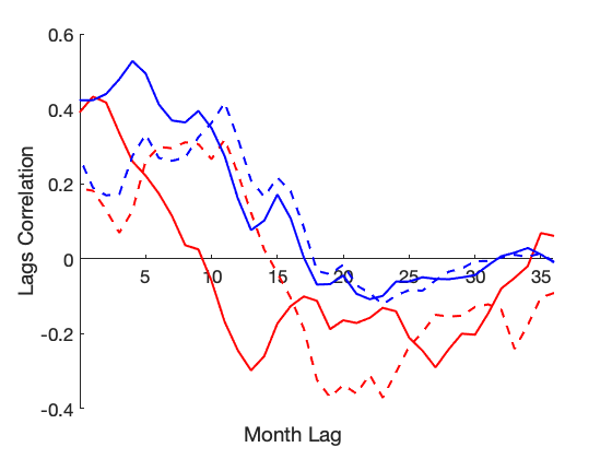
Lead–lag correlation analysis presents the lag (in months) between the peak of ENSO and the SST and SSS in the Agulhas Leakage region (box 1 in Figure 1). SST and SSS for the La Niña years have a stronger correlation than the El Niño year. SST and SSS for the El Niño years behave independently instead of mirroring the trend of the other. SST and SSS of La Niña have a positive correlation with the ONI until approximately 17 months after the peak of the event (Figure 9). Both variables continue to negatively correlate after this mark until about 32 months when the correlation becomes slightly positive. The SST for the La Niña events peaks positively at about 5 months and the SSS at about 12 months. The SST for El Niño is positively correlated until about 10 months and remains negative until about 34 months after the peak of the event. The SSS of El Niño is positively correlated with the ONI until about 14 months and remains negatively correlated for the rest of the period. The positive peak of SST for El Niño is at about 2 months and the SSS is less dramatic, plateauing around 5 to 11 months. Figure 9 supports the idea of SST changing faster than SSS as both lines of SST become negatively correlated prior to those of SSS.
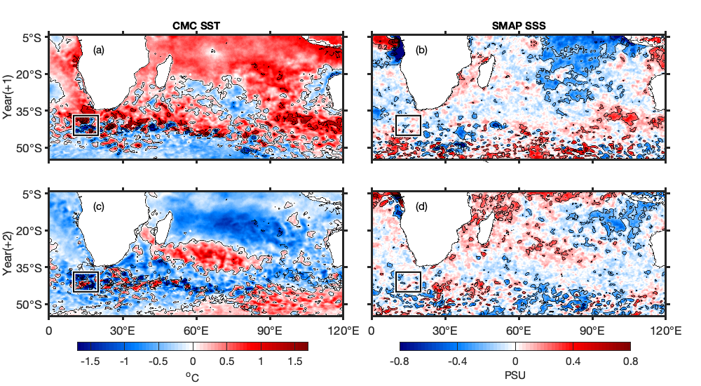
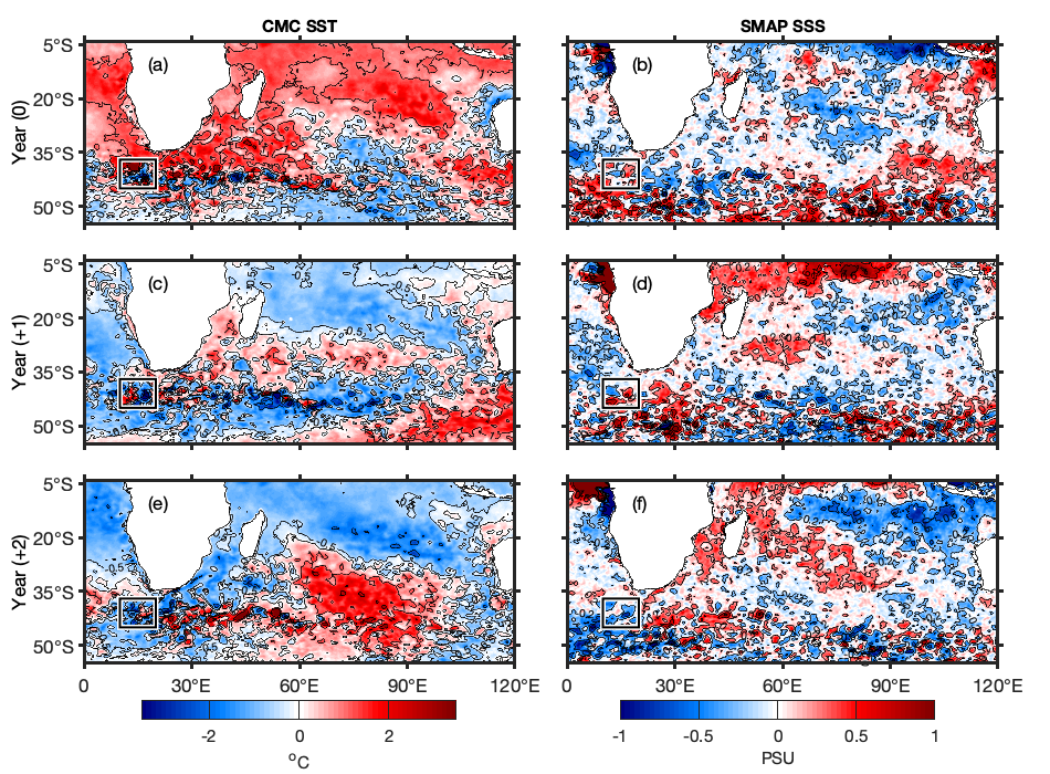
SSH, SST, and SSS anomalies are plotted in 2015 (an El Niño year) and two years later in 2017 (Figure 10). The SSH anomalies vary throughout the entire region in both panels, but the difference is more dramatic in Figure 10b that has stronger anomalies than Figure 10a. Warm waters from El Niño induce thermal expansion and anomalously high SSH anomalies. There is a noticeable change from Figure 10c to Figure 10d where the domain anomalously warms, as expected after an El Niño [19]. The Agulhas Current is anomalously warm in Figure 10d compared with Figure 8. Anomalously warm waters in the northwestern part of Figure 10c are observed moving into the Mozambique Channel and then into the Agulhas Current. From Figure 10e,f, saline regions become more saline, and the fresh regions become fresher. In 2017 (Figure 4d), there is an increase in salinity, similar to the increase in salinity of the saline regions from Figure 10e to Figure 10f.
SSH, SST, and SSS anomalies during the 2016 La Niña event and two years later in 2018 (Figure 11) reveal a decrease in SSH anomalies in the northwestern region from Figure 11a to Figure 11b, signifying the effects of the La Niña signal traveling through the ITF and propagating towards Africa via the South Equatorial Current [20,24]. Cold waters enter the region around 90° E in Figure 11c where the Subtropical Front (STF) joins the ARC and recirculates into the Agulhas Current [25].
3.2. Subsurface Properties
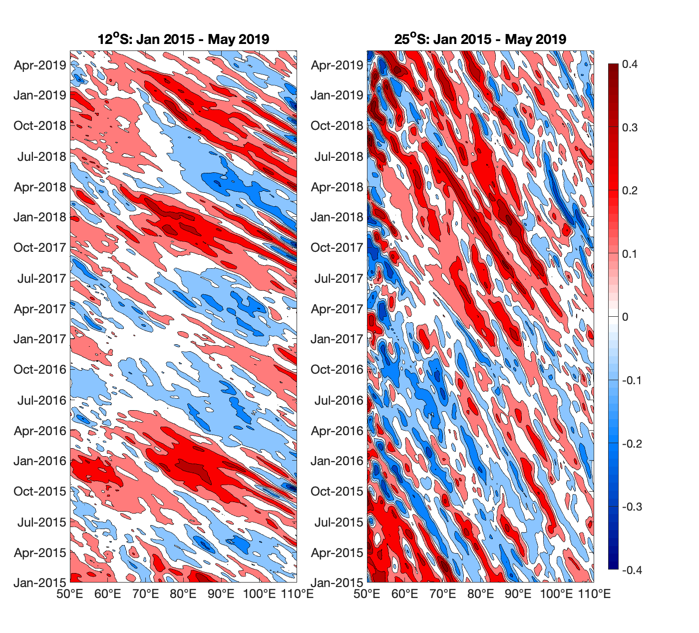
A Hovmöller diagram of SSH anomalies at 12° S and 25° S from 50° to 100° W during January 2015 to May 2019 presents alternating bands of negative and positive SSH anomalies, signifying westward propagation of Rossby waves (Figure 12). The angle of the bands is steeper at 25° S than at 12° S because the Rossby waves propagate faster at this latitude. In the 12° S diagram, there is westward movement of water masses consistent with ENSO events. There is a large mass of positively anomalous water appearing in 2016, one year after the 2015 El Niño. Anomalously warm waters in Figure 4a at this time contribute to thermal expansion and increased SSH anomalies. A mass of anomalously negative water appears in 2018 two years after the 2016 La Niña and may be attributed to that event. In the 25° S diagram, the large portion of anomalously positive bands may be attributed to the 2015 El Niño, and the effects took longer to reach this region because of ocean circulation patterns [26].
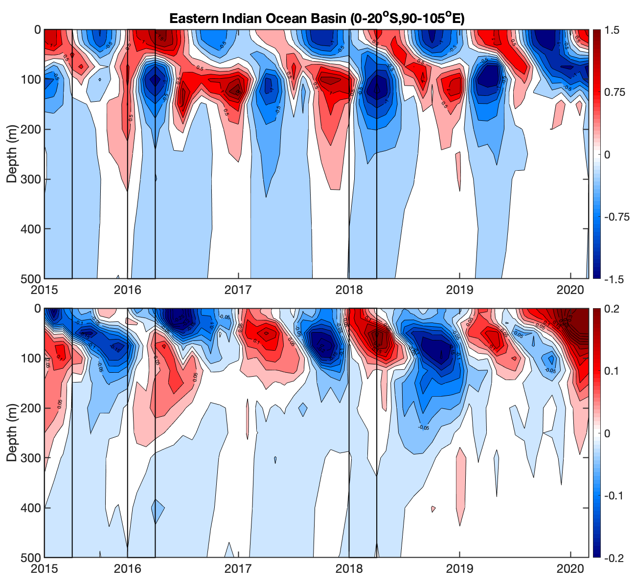
The depth–time plots in Figure 13 present Argo temperature (top panel) and salinity (bottom panel) anomalies in the eastern Indian Ocean from April 2015 to March 2020 (box 5 in Figure 1). Figure 13, Figure 14 and Figure 15 allow us to evaluate temperature and salinity anomalies as a function of depth in the upper 500 m. The temperature and salinity in Figure 13 are in antiphase; when there are colder temperatures, there are higher salinities and vice versa. The salinity lags behind temperature, which would further support the conclusion that salinity changes later than temperature from Figure 2, Figure 3 and Figure 4. The boxes in the diagram represent January–March of ENSO years. This region experiences the effects of ENSO events first because it is geographically closest to the Pacific where ENSO events originate (box 5 in Figure 1) [27]. There are anomalously warm temperatures at the surface in the eastern Indian Ocean in 2016 (Figure 4a), which are observed in Figure 13 as well and may be attributed to the 2015 El Niño. This anomalously warm mass of water begins in late 2015 from the surface up to 300 m depth and continues into early 2017. We expect to see temporal effects in this region a year after a La Niña event (Figure 2c and Figure 3c), which is also supported in this diagram. Figure 2d shows anomalously saline waters in this region in 2017 in the bottom panel of Figure 13. This anomalously saline mass of water reaches down to about 150 m. The response in salinity for the La Niña events is two to three years after the event (Figure 2 and Figure 3e,g). This is displayed in Figure 13 by the large mass of anomalously fresh water in the second half of 2019. This mass of water extends to approximately 300 m deep.
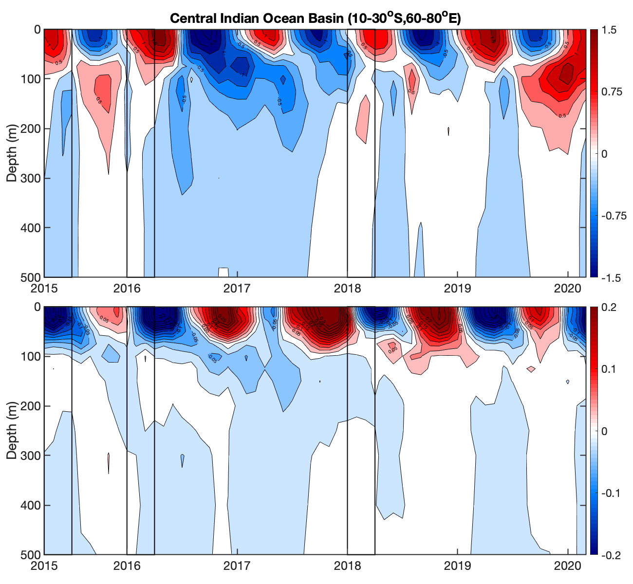
Subsurface variations in Argo temperature (top panel) and salinity (bottom panel) anomalies in the central Indian Ocean (box 4 in Figure 1) from April 2015 to March 2020 are presented in Figure 14. The effects of the El Niño event and La Niña events appear around the same time as in Figure 13, but a little later and in different intensities. The surface temperature and salinity also generally do not reach as deep down in this region as they did in Figure 13 in the eastern Indian Ocean due to the different stratification of the local water column [26]. The general temperature change is very similar to that in Figure 11. The salinity follows the same pattern as Figure 13 but experiences stronger variability due to the South Equatorial Current and both the Northeast and Southeast Madagascar Currents (NEMC, SEMC). Theses currents transport high volumes of water; the NEMC transports about 30 Sv and the SEMC transports about 20 Sv [26].
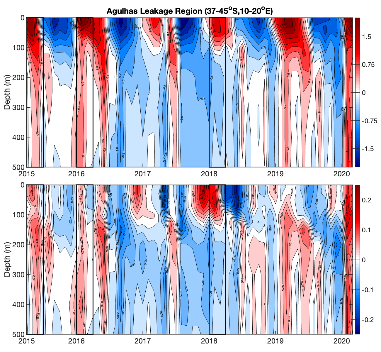
Subsurface Argo temperature (top panel) and salinity (bottom panel) anomalies in the Agulhas Leakage region from April 2015 to March 2020 are displayed in Figure 15. Both temperature and salinity changes experience higher variability than the regions in Figure 13 and Figure 14. This is expected because the Agulhas Current advects waters with different temperature and salinity characteristics [25]. The temperature changes seasonally, and the salinity appears to be in antiphase with the temperature with a small lag. The temperature and salinity extend much further than in Figure 13 and Figure 14, even reaching 500 m, because the Agulhas Current has large vertical transports [28]. Since this region is the furthest from the Pacific out of the three depth plots, it is expected that the effects of ENSO will arrive later [26,27]. There is an increase in SST in this region in Figure 4a one year after the 2015 El Niño, which can be seen in the top panel of this diagram, and it extends all the way to 500 m. Anomalously cool waters flow along the Agulhas Current two years after the La Niña events (Figure 3e), but there are anomalously warm waters in the Agulhas Leakage region at this time. The leakage region may not have been majority anomalously cool until just after this, which is seen in the top panel of Figure 14, in 2019. The leakage region is not anomalously saline until three years after the 2015 El Niño and anomalously fresh three years after the La Niña events (Figure 2 and Figure 3). There is a mass of anomalously saline water three years after the El Niño in 2018 which only extends slightly beyond 100 m depth. At the beginning of 2019, three years after the 2016 La Niña, there is both anomalously saline and fresh waters, which aligns with the region in Figure 3g.
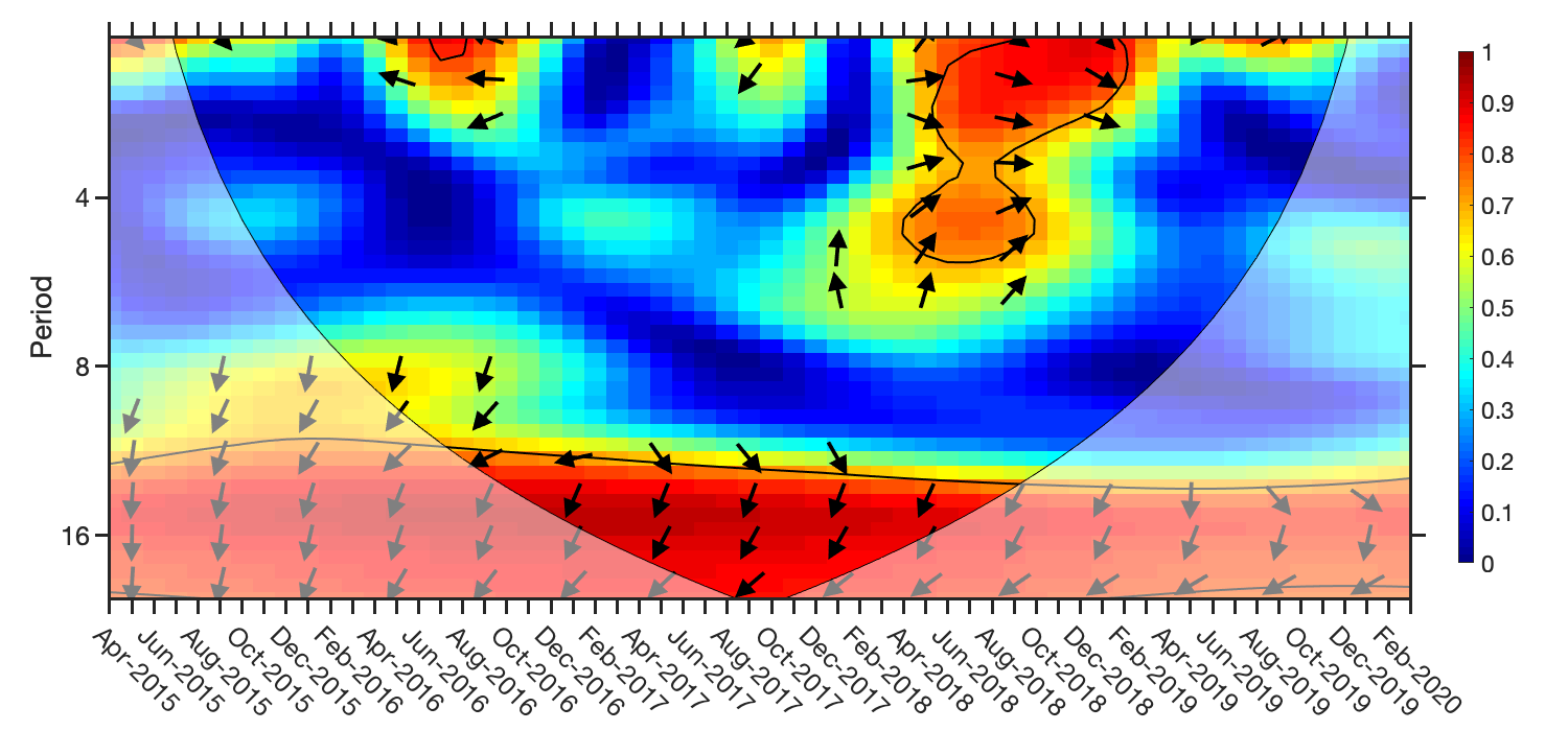
Wavelet analysis of SSS and ENSO (via the Oceanic Niño Index) was conducted in the Agulhas Leakage region (Figure 16). There are three regions of high correlation in this plot. One appears in about June 2016, a second centered about May 2018, and a third for all months for periodicities higher than 12 months. This first region directly relates to the 2015 El Niño, and the second region may be the effects of the 2016 La Niña once the signal has propagated to the Agulhas Current region. The arrows pointing left in the first region of high correlation mean SSS and ENSO are out of phase, and they slightly point up, meaning that the Oceanic Niño Index leads SSS, though the statistically significant region is only for periods of 1–2 months, so this is likely not an immediate ENSO–Agulhas response. In the second region, the arrows point right, meaning ENSO and SSS are in phase, and they slightly point down in the upper part of the region and up in the lower part. This reveals that ENSO led SSS and then the statistical relationship switched to where SSS leads ENSO. This second event has a statistically significant correlation for periods of up to 5 months. The main takeaway from this analysis is that there is a consistent statistically significant correlation between ENSO and SSS on timescales longer than one year, and also isolated events of positive correlations on interannual timescales, which are likely attributed to the lagged effect between SSS in the Agulhas Current region and each individual ENSO event to permit the signal to propagate across the Indian Ocean and through the Mozambique Channel. However, the persistent long-term correlation is optimistic for justification of this study and the effectiveness of SMAP on understanding Agulhas Current and ENSO interactions.
4. Discussion and Conclusions
We studied the effects of ENSO events on SST and SSS in the Agulhas Current for the first time focusing on the SMAP satellite era. SMAP is the newest salinity satellite and spans multiple ENSO events with a long enough temporal coverage to trace the propagating ENSO signals across the Indian Ocean, southward through the Mozambique Channel, and into the Agulhas Current region. We found an anomalously warm and saline response after an El Niño event and an anomalously cool and fresh response after a La Niña event. This is consistent with results from other studies [5,12], though this is the first study that uses the novel SMAP SSS satellite for this purpose. As there are other factors such as the Indian Ocean Dipole [22], we cannot say ENSO has an exact correlation with the changes in salinity and temperature seen in this study, but there is a consistent surface temperature and salinity response that we identified spatially and temporally within the Agulhas Current region, but also along Rossby waves that transmit the signal westward across the Indian Ocean. The change in SST in the Agulhas Current region after an ENSO event is strongest about a year after each event, and the change in SSS is strongest approximately two years after. We noted a dipolar signal that completely reverses as the signal reaches the retroflection region, but the pathways are slightly different in CMC SST and SMAP SSS. While both propagate southward through the Mozambique Channel, SSS is the only parameter that also illustrates a pathway along the eastern coast of Madagascar, consistent with the flow of the Indian Ocean Gyre. We confirmed these findings and pathways through a time series analysis and a lead–lag analysis and found that temperature and salinity correlate best in the Agulhas Leakage region compared to other subregions in the selected domain (Mozambique Channel, etc.), likely due to water mass trapping and transport by rings.
SST and SSS of La Niña have a positive correlation with the ONI until about 17 months after the peak of the event. In all scenarios, the SSS of El Niño is positively correlated with the ONI until about 14 months and remains negatively correlated for the rest of the period. The positive peak of SST for El Niño is at about 2 months, and the SSS is less dramatic, plateauing around 5 to 11 months. The change in SSS appearing two years after an event is consistent with findings by Paris et al. [12], but the SST changing in a year is faster than their results, indicating that the lag time between the Agulhas SST and ENSO events may be decreasing, signifying a faster response.
We tracked Rossby waves and their propagation across the Indian Ocean and observed alternating bands of negative and positive SSH anomalies and consistent westward propagation. The strongest mass of anomalously negative SSH anomalies appears in 2018, which would be two years after the 2016 La Niña and may be attributed to that event. In the 25° S diagram, the large portion of anomalously positive bands may be attributed to the 2015 El Niño as well, but it took longer for the effects to reach this region because of ocean circulation patterns [26]. We then observed temperature and salinity with depth. The temperature and salinity in Figure 11 are in antiphase; when there are colder temperatures, there are higher salinities, and vice versa. There are anomalously warm temperatures at the surface in the eastern Indian Ocean in 2016. This anomalously warm mass of water begins in late 2015, reaching more than 300 m depth, and continues into 2017. The response in salinity for the La Niña events is approximately two to three years after the event (Figure 3e,g). This mass of water reaches down to about 300 m in depth. A wavelet coherence analysis of SSS and ENSO (via the Oceanic Niño Index) in the Agulhas Leakage region revealed a persistent long-term correlation (of periods greater than 12 months), which is optimistic for justification of this study and the effectiveness of SMAP on understanding Agulhas Current and ENSO interactions. SMAP is a novel SSS satellite and the findings of this work may perhaps help lay the groundwork for prediction of ENSO-related SSS signals in the Agulhas Current region for future events in the salinity satellite era. It would be interesting to see similar work that focuses on a real-time ENSO event using near-real-time SMAP SSS data as a possible perspective research axis of this work.
Author Contributions
Conceptualization, C.B.T., B.S., and C.E.W.; methodology, C.B.T.; software, C.B.T. and C.E.W.; validation, C.B.T., B.S., and C.E.W.; formal analysis, C.B.T. and C.E.W.; investigation, C.B.T. and C.E.W.; resources, B.S.; data curation, C.B.T.; writing—original draft preparation, C.B.T. and C.E.W.; writing—review and editing, C.B.T., B.S., and C.E.W.; visualization, C.B.T. and C.E.W.; supervision, C.B.T. and B.S.; project administration B.S.; funding acquisition, B.S. All authors have read and agreed to the published version of the manuscript.
Funding
This research was funded by the United States Office of Naval Research Award #N00014-20-1-2742, awarded to B.S.
Data Availability Statement
The authors acknowledge the various data sources for the freely available data. The Argo data are provided by the APRDC (http://apdrc.soest.hawaii.edu/datadoc/argo_iprc_gridded.php, accessed on 21 April 2021). The SMAP data used for this study are the Level 3 version 4.3 provided by NASA’s Jet Propulsion Laboratory (https://podaac.jpl.nasa.gov/announcements/2020-03-18_JPL_SMAP_SSS_CAP_Dataset_Release, accessed on 21 April 2021). The GHRSST data used are provided by the Canadian Meteorological Centre (https://podaac.jpl.nasa.gov/dataset/CMC0.2deg-CMC-L4-GLOB-v2.0, accessed on 21 April 2021). The SSH anomaly data in this study are provided by CMEMS (https://resources.marine.copernicus.eu/?option=com_csw&task=results&product_id=SEALEVEL_GLO_PHY_L4_REP_OBSERVATIONS_008_047&view=details, accessed on 21 April 2021). The ENSO event data are determined by the ONI provided by the National Weather Service Climate Prediction Center (https://origin.cpc.ncep.noaa.gov/products/analysis_monitoring/ensostuff/ONI_v5.php, accessed on 21 April 2021).
Acknowledgments
We are thankful for the helpful comments of the four anonymous reviewers which improved the quality of this paper. This is NRL contribution number JA-7320-21-5165. It is approved for public release; distribution is unlimited.
Conflicts of Interest
The authors declare no conflict of interest. The funders had no role in the design of the study; in the collection, analyses, or interpretation of data; in the writing of the manuscript, or in the decision to publish the results.
References
- Lutjeharms, J.R.E.; Van Ballegooyen, R.C. The Retroflection of the Agulhas Current. J. Phys. Oceanogr. 1988, 18, 1570–1583. [Google Scholar] [CrossRef]
- Simon, M.H.; Arthur, K.L.; Hall, I.R.; Peeters, F.J.C.; Loveday, B.R.; Baker, S.; Ziegler, M.; Zahn, R. Millennial-scale Agulhas Current variability and its implications for salt-leakage through the Indian-Atlantic Ocean Gateway. Earth Planet. Sci. Lett. 2013, 383, 101–112. [Google Scholar] [CrossRef]
- Biastoch, A.; Boning, C.W.; Lutjeharms, R.E. Agulhas leakage dynamics affects decadal variability in Atlantic overturning circulation. Nature 2008, 456, 489–492. [Google Scholar] [CrossRef] [PubMed]
- Ezer, E.; Mellor, G.L. Simulations of the Atlantic Ocean with a free surface sigma coordinate ocean model. J. Geophys. Res. 1997, 102, 15647–15657. [Google Scholar] [CrossRef] [Green Version]
- Putrasahan, D.; Kirtman, B.P.; Beal, L.M. Modulation of SST Interannual Variability in the Agulhas Leakage Region Associated with ENSO. J. Clim. 2016, 29, 7089–7102. [Google Scholar] [CrossRef]
- Weijer, W.; De Ruijter, W.P.M.; Sterl, A.; Drijfhout, S.S. Response of the Atlantic overturning circulation to South Atlantic sources of buoyancy. Glob. Planet. Chang. 2002, 34, 293–311. [Google Scholar] [CrossRef]
- Beal, L.M.; De Ruijter, W.P.M.; Biastoch, A.; Zahn, R. On the role of the Agulhas system in ocean circulation and climate. Nature 2011, 472, 429–436. [Google Scholar] [CrossRef] [PubMed]
- Krishnamurthy, V.; Kirtman, B.P. Variability of the Indian Ocean; Relation to monsoon and ENSO. Q. J. R. Meteorol. Soc. 2003, 129, 1623–1646. [Google Scholar] [CrossRef]
- Murtugudde, R.; Busalacchi, A.J.; Beauchamp, J. Seasonal-to-Interannual effects of the Indonesian Throughflow on the tropical Indo-Pacific Basin. J. Geophys. Res. 1998, 103, 21425–21441. [Google Scholar] [CrossRef]
- Elipot, S.; Beal, L.M. Observed Agulhas Current Sensitivity to Interannual and Long-Term Trend Atmosphere Forcings. J. Clim. 2018, 31, 3077–3098. [Google Scholar]
- Paris, M.L.; Subrahmanyam, B.; Trott, C.B.; Murty, V.S.N. Influence of ENSO Events on the Agulhas Leakage Region. Remote Sens. Earth Syst. Sci. 2018, 1, 79–88. [Google Scholar] [CrossRef]
- Paris, M.L.; Subrahmanyam, B. Role of El Niño Southern Oscillation (ENSO) Events on Temperature and Salinity Variability in the Agulhas Leakage Region. Remote Sens. 2018, 10, 127. [Google Scholar]
- Vazquez-Cuervo, J.; Gentemann, C.; Tang, W.; Carroll, D.; Zhang, H.; Menemenlis, D.; Gomez-Valdes, J.; Bouali, M.; Steele, M. Using Salidrones to Validate Arctic Sea-Surface Salinity from the SMAP Satellite and from Ocean Models. Remote Sens. 2021, 13, 831. [Google Scholar] [CrossRef]
- Fore, A.G.; Yueh, S.H.; Tang, W.; Stiles, B.W.; Hayashi, A.K. Combined Active/Passive Retrievals of Ocean Vector Wind and Sea Surface Salinity With SMAP. IEEE Trans. Geosci. Remote Sens. 2016, 54, 7396–7404. [Google Scholar] [CrossRef]
- Fiedler, E.K.; McLaren, A.; Banzon, V.; Brasnett, B.; Ishizaki, S.; Kennedy, J.; Rayner, N.; Roberts-Jones, J.; Corlett, G.; Merchant, C.J.; et al. Intercomparison of long-term sea surface temperature analyses using the GHRSST Multi-Product Ensemble (GMPE) system. Remote Sens. Environ. 2019, 222, 18–33. [Google Scholar] [CrossRef] [Green Version]
- Wang, T.; He, H.; Fan, D.; Fu, B.; Dong, S. Global ocean mesoscale vortex recognition based on DeeplabV3plus model. Conf. Ser. Earth Environ. Sci. 2021, 671, 012001. [Google Scholar]
- Du, Y.; Zhang, Y. Satellite and Argo Observed Surface Salinity Variations in the Tropical Indian Ocean and Their Association with the Indian Ocean Dipole Mode. J. Clim. 2015, 28, 695–713. [Google Scholar] [CrossRef] [Green Version]
- Grinsted, A.; Moore, J.C.; Jerejeva, S. Application of the cross wavelet transform and wavelet coherence to geophysical time series. Nonlinear Process. Geophys. 2004, 11, 561–566. [Google Scholar] [CrossRef]
- Roman-Stork, H.L.; Bulusu, S.; Trott, C.B. Mesoscale eddy variability and its linkage to deep convection over the Bay of Bangel using satellite altimetric observations. Adv. Space Res. 2019. [Google Scholar] [CrossRef]
- Sebille, E.V.; Sprintall, J.; Schwarzkopf, F.U.; Gupta, A.S.; Santoso, A.; England, M.H.; Biastoch, A.; Boning, C.W. Pacific-to-Indian Ocean connectivity: Tasman leakage, Indonesian Throughflow, and the role of ENSO. J. Geophys. Res. Ocean. 2014, 119, 1365–1382. [Google Scholar] [CrossRef] [Green Version]
- Jensen, T.G. Arabian Sea and Bay of Bengal exchange of salt and tracers in an ocean model. Geophys. Res. Lett. 2001, 28, 3967–3970. [Google Scholar] [CrossRef]
- Grunseich, G.; Subrahmanyam, B.; Murty, V.S.N.; Giese, B.S. Sea surface salinity variability during the Indian Ocean Dipole and ENSO events in the tropical Indian Ocean. J. Geophys. Res. 2011, 116. [Google Scholar] [CrossRef] [Green Version]
- National Weather Service Climate Prediction Center. Available online: https://origin.cpc.ncep.noaa.gov/products/analysis_monitoring/ensostuff/ONI_v5.php (accessed on 10 March 2021).
- Gordon, A.L.; Ma, S.; Olson, D.B.; Hacker, P.; Ffield, A.; Talley, L.D.; Wilson, D.; Baringer, M. Advection and diffusion of Indonesian Throughflow Water within the Indian Ocean South Equatorial Current. Geophys. Res. Lett. 1997, 24, 2573–2576. [Google Scholar] [CrossRef] [Green Version]
- Lutjeharms, J.R.E.; Ansorge, I.J. The Agulhas Return Current. J. Mar. Syst. 2001, 30, 115–138. [Google Scholar] [CrossRef]
- Schott, F.A.; Xie, S.P.; McCreary, J.P., Jr. Indian Ocean Circulation and Climate Variability. Rev. Geophys. 2009, 47. [Google Scholar] [CrossRef]
- Cai, W.; Meyers, G.; Shi, G. Transmission of ENSO signal to the Indian Ocean. Geophys. Res. Lett. 2005, 32. [Google Scholar] [CrossRef]
- Bryden, H.L.; Beal, L.M.; Duncan, L.M. Structure and Transport of the Agulhas Current and Its Temporal Variability. J. Oceanogr. 2004, 61, 479–492. [Google Scholar] [CrossRef]
Figure 1.
Climatological mean (a) SMAP SSS (psu), (b) CMC SST (°C), and (c) CMEMS SSH anomalies (m) and geostrophic current vectors for the period of 2016–2020. The period selected for the climatology is to include full years of SMAP SSS data and eliminate seasonal bias. Major features are labeled in panel (c). ITF = Indonesian Throughflow, Agulhas Retroflection, Agulhas Current, Agulhas Return Current, and Rossby waves. Bathymetry in panel (a) is contoured every 2500 m. Boxes 1 through 5 are referenced throughout the text and signify regions of interest.

Figure 2.
The 2016 La Niña events from January to March for both Canadian Meteorological Centre (CMC) sea surface temperature (SST) anomalies (left column, °C) and Soil Moisture Active Passive (SMAP) sea surface salinity (SSS) anomalies (right column, psu) during the peak (a,b), the following year (c,d), and two years after (e,f). The boxes represent the leakage region (37°–45° S, 10°–20° E, box 1 in Figure 1). Contours are labeled to reflect exact values.

Figure 3.
The 2018 La Niña events from January to March for both Canadian Meteorological Centre (CMC) sea surface temperature (SST) anomalies (left column, °C) and Soil Moisture Active Passive (SMAP) sea surface salinity (SSS) anomalies (right column, psu) during the peak (a,b), the following year (c,d), and two years after (e,f). The boxes represent the leakage region (37°–45° S, 10°–20° E, box 1 in Figure 1). Contours are labeled to reflect exact values.

Figure 4.
Same as Figure 2 and Figure 3 but for the 2015 El Niño during the following year (a,b) and two years after (c,d). Contours are labeled to reflect exact values.

Figure 5.
Composite mean of SMAP SSS anomalies for 2016 and 2018 La Niña events (left column, psu) and 2015 El Niño event (right column, psu) two years after the peak for Apri–June (a,b), July–September (c,d), October–December (e,f), and three years after the peak for January–March (g,h). The boxes represent the leakage region (37°–45° S, 10°–20° E, box 1 in Figure 1). Contours are labeled to reflect exact values.

Figure 6.
Composite mean for 2016 La Niña event from January–March for both CMC SST anomalies (left column, °C) and SMAP SSS anomalies (right column, psu) during the peak (a,b), the following year (c,d), and two years after (e,f). The boxes represent the leakage region (37°–45° S, 10°–20° E, box 1 in Figure 1). Contours are labeled to reflect exact values.

Figure 7.
Composite mean for weak 2016 La Niña event minus the slightly less weak 2018 La Niña event from January to March for both CMC SST anomalies (left column, °C) and SMAP SSS anomalies (right column, psu) during the peak (a,b), the following year (c,d), and two years after (e,f). The boxes represent the leakage region (37°–45° S, 10°–20° E, box 1 in Figure 1). Contours are labeled to reflect exact values.

Figure 8.
Time series from 2016 to 2020 for region north of Madagascar (0°–20° S, 35°–65° E, top panel, box 3 in Figure 1), region between Madagascar and the coast of Africa (15°–25° S, 35°–45° E, middle panel, box 3 in Figure 1), and monthly boxed average (37°–45° S, 10°–20° E, bottom panel, box 1 in Figure 1) CMC SST (solid line, °C) and SMAP SSS (dashed line, psu) anomalies. ENSO events are represented during their peak (January–March) by vertical shaded bars.

Figure 9.
Correlation analysis between absolute values of the Oceanic Niño Index (ONI) and box-averaged CMC SST anomalies (solid line, °C) and between ONI and box-averaged SMAP SSS anomalies (dashed line, psu) at monthly lag intervals for El Niño years in red and La Niña years in blue.
Figure 9.
Correlation analysis between absolute values of the Oceanic Niño Index (ONI) and box-averaged CMC SST anomalies (solid line, °C) and between ONI and box-averaged SMAP SSS anomalies (dashed line, psu) at monthly lag intervals for El Niño years in red and La Niña years in blue.

Figure 10.
CMEMS SSH anomalies (a,b; m), CMC SST (c,d; °C), and SMAP SSS (e,f; psu) anomalies averaged from January to March during the peak of the 2015 El Niño event (a,c,e) and two years following (b,d,f). Contours are labeled to reflect exact values.
Figure 10.
CMEMS SSH anomalies (a,b; m), CMC SST (c,d; °C), and SMAP SSS (e,f; psu) anomalies averaged from January to March during the peak of the 2015 El Niño event (a,c,e) and two years following (b,d,f). Contours are labeled to reflect exact values.

Figure 11.
CMEMS SSH anomalies (a,b; m), CMC SST (c,d; °C), and SMAP SSS (e,f; psu) anomalies averaged from January to March during the peak of the 2016 La Niña event (a,c,e) and two years following (b,d,f). Contours are labeled to reflect exact values.
Figure 11.
CMEMS SSH anomalies (a,b; m), CMC SST (c,d; °C), and SMAP SSS (e,f; psu) anomalies averaged from January to March during the peak of the 2016 La Niña event (a,c,e) and two years following (b,d,f). Contours are labeled to reflect exact values.

Figure 12.
Hovmöller diagrams from CMEMS SSH anomalies (m) at 12° S (left) and 25° S (right) from January 2015 to May 2019.
Figure 12.
Hovmöller diagrams from CMEMS SSH anomalies (m) at 12° S (left) and 25° S (right) from January 2015 to May 2019.

Figure 13.
Depth–time sections of box-averaged Argo temperature anomalies (top panel, °C) and Argo salinity anomalies (bottom panel, psu) from April 2015 to March 2020 in the eastern Indian Ocean basin (0°–20° S, 90°–105° E, box 5 in Figure 1).
Figure 13.
Depth–time sections of box-averaged Argo temperature anomalies (top panel, °C) and Argo salinity anomalies (bottom panel, psu) from April 2015 to March 2020 in the eastern Indian Ocean basin (0°–20° S, 90°–105° E, box 5 in Figure 1).

Figure 14.
Depth–time sections of box-averaged Argo temperature anomalies (top panel, °C) and Argo salinity anomalies (bottom panel, psu) from April 2015 to March 2020 in the central Indian Ocean basin (10°–30° S, 60°–80° E, box 4 in Figure 1).
Figure 14.
Depth–time sections of box-averaged Argo temperature anomalies (top panel, °C) and Argo salinity anomalies (bottom panel, psu) from April 2015 to March 2020 in the central Indian Ocean basin (10°–30° S, 60°–80° E, box 4 in Figure 1).

Figure 15.
Depth–time sections of box-averaged Argo temperature anomalies (top panel, °C) and Argo salinity anomalies (bottom panel, psu) from April 2015 to March 2020 in the Agulhas Leakage region (37°–45° S, 10°–20° E, box 1 in Figure 1).
Figure 15.
Depth–time sections of box-averaged Argo temperature anomalies (top panel, °C) and Argo salinity anomalies (bottom panel, psu) from April 2015 to March 2020 in the Agulhas Leakage region (37°–45° S, 10°–20° E, box 1 in Figure 1).

Figure 16.
Wavelet analysis between monthly box-averaged SMAP SSS anomalies (psu) and absolute values of Oceanic Niño Index (ONI) in the Agulhas Leakage region (37°–45° S, 10°–20° E). Arrows represent phase angle: pointing down indicates that SSS leads ENSO, pointing up indicates that ENSO leads SSS, pointing right indicates they are in phase, and pointing left indicates they are out of phase.

Publisher’s Note: MDPI stays neutral with regard to jurisdictional claims in published maps and institutional affiliations. |
© 2021 by the authors. Licensee MDPI, Basel, Switzerland. This article is an open access article distributed under the terms and conditions of the Creative Commons Attribution (CC BY) license (https://creativecommons.org/licenses/by/4.0/).
Share and Cite
MDPI and ACS Style
Trott, C.B.; Subrahmanyam, B.; Washburn, C.E. Investigating the Response of Temperature and Salinity in the Agulhas Current Region to ENSO Events. Remote Sens. 2021, 13, 1829. https://0-doi-org.brum.beds.ac.uk/10.3390/rs13091829
AMA Style
Trott CB, Subrahmanyam B, Washburn CE. Investigating the Response of Temperature and Salinity in the Agulhas Current Region to ENSO Events. Remote Sensing. 2021; 13(9):1829. https://0-doi-org.brum.beds.ac.uk/10.3390/rs13091829
Chicago/Turabian StyleTrott, Corinne B., Bulusu Subrahmanyam, and Caroline E. Washburn. 2021. "Investigating the Response of Temperature and Salinity in the Agulhas Current Region to ENSO Events" Remote Sensing 13, no. 9: 1829. https://0-doi-org.brum.beds.ac.uk/10.3390/rs13091829
Note that from the first issue of 2016, this journal uses article numbers instead of page numbers. See further details here.