
Operational Processing of Big Satellite Data for Monitoring Glacier Dynamics: Case Study of Muldrow Glacier


Canada Centre for Mapping and Earth Observation, Natural Resources Canada, 560 Rochester Street, Ottawa, ON K1S 5K2, Canada
Remote Sens. 2022, 14(11), 2679; https://0-doi-org.brum.beds.ac.uk/10.3390/rs14112679
Submission received: 29 April 2022
/
Revised: 28 May 2022
/
Accepted: 1 June 2022
/
Published: 3 June 2022
(This article belongs to the Special Issue Remote Sensing of the Cryosphere)
Abstract
:Frequent acquisition of Synthetic Aperture Radar (SAR) data by the European Sentinel-1 satellites provides an opportunity for monitoring the dynamics of worldwide glaciers. We present a fully-automated processing system for producing multi-dimensional time series of glacier flow. We then use this fully-automated processing system to investigate the dynamics of Muldrow Glacier, located in the Denali National Park and Preserve (Alaska, AK, USA) during the October 2014—November 2021 period. We compute north, east, and vertical Surface-Parallel-Flow (SPF) and non-Surface-Parallel-Flow (nSPF) components of flow velocity and displacement with an average temporal resolution of 9 days and grid spacing of 100 m. During this period, we observe a glacier surge, a manifold increase in glacier flow velocity, that started as early as 2017 and continues until the present; however, the near completion of this surge is apparent. This glacier previously surged in 1906–1912 (the exact date is unknown) and in 1956–1957. We present our results in different ways to emphasize various aspects of the observed surge and demonstrate the full capability of our processing system. As the availability of SAR data improves, we expect that the fully-automated processing systems, similar to the one presented here, will play an increasingly dominant role and soon entirely replace manual processing.
1. Introduction
Regular, high-frequency observations of remote glaciers with modern spaceborne Synthetic Aperture Radars (SAR) provide an opportunity to study glacier dynamics with high spatial and temporal resolutions. At many glaciers, ice velocity is either constant or changes slowly; however, some glaciers experience a rapid increase in ice velocity lasting from a few days to a few years, known as glacier surge [1]. Glacier surges produce a rapid redistribution of ice resulting in the upper part of a glacier becoming thinner and the lower part of a glacier becoming thicker. At those glaciers, surges repeat at nearly constant intervals, with the time in between the surges required for ice accumulation at the upper part of a glacier before the next surge. Climate change affects accumulation and ablation at a glacier and the established intervals between the consecutive surges. Before the epoch of instrumental observations, many surges at remote glaciers were poorly documented or completely missed.
Muldrow Glacier is located on the northern slope of the Alaska Range near Mt. McKinley, the highest mountain peak in North America, with an elevation of over 6100 m (Figure 1). This glacier, with an area of 393 km2 and a length of 63 km, starts at 6100 m elevation and abruptly descends to 2000 m, then more gradually to 800 m. The glacier meets its largest tributary, the Traleika Glacier, at 1700 m elevation, and the Brooks Glacier at 1600 m elevation. Below these tributaries, the glacier is uniform, with a width of about 2.5 km. The upper portion of the glacier flows in the northeasterly direction for 42 km and then turns to the northwestern direction [2].
Morainal patterns on Muldrow Glacier indicate that at least four surges (in addition to the one studied here) occurred during the past 200 years [3]. The most recent documented surge occurred during the winter of 1956–1957, with surface ice displacements over 6.6 km. This surge produced a lowering by at least 170 m of the surface at the upper portion of the glacier and a rise in the terminal portion, with the roughly equal net exchange of ice [2]. An earlier surge at this glacier occurred sometime between 1906 and 1912 [4]. In all the cases it was unknown whether these surges began rapidly or gradually.
We pursue two objectives in this study. The first objective is to demonstrate the capabilities of our fully-automated processing system that has already been tested on many glaciers in Alaska and Yukon [5,6] and to describe characteristics that define its performance and quality of results. The second objective is to show the dynamics of a recent surge of the Muldrow Glacier—the first surge of this glacier ever observed with the modern remote sensing techniques.
2. Data and Methodology
To start the processing, it is sufficient to specify Sentinel-1 track(s) and frame(s) in the Alaska Satellite Facility (ASF) notation and desired resolution (in terms of multilooking, see below) of the final products. The processing flow is controlled by the BASH scripts, which call executables written in C++ and python. Individual range and azimuth offset maps are computed with the help of GAMMA software [7]. The processing is typically performed on a High-Performance Computer (HPC) Linux cluster but it can also be performed on a powerful Linux workstation. One data set (that can consist of more than one frame) is processed as a single job, and multiple jobs can be submitted in parallel. On HPC we typically allocate ten nodes of forty cores each for a job (400 cores in total), but this number can vary depending on resource availability, which results in an almost linear increase or decrease in processing time. Computation of range/azimuth offset maps within a single job is performed by parallel processes. Typically each process uses ten cores, therefore, forty range/azimuth offset maps can be computed simultaneously. With these processing resources, it takes 1–2 days to process a typical Sentinel-1 set of about 150 single-frame images.
In this study, we use 135 ascending (track 065) and 164 descending (track 131) Sentinel-1 Interferometric Wide (IW) single-look complex (SLC) images with 2.3 m (range) × 14.9 m (azimuth) spatial resolution from the NASA Distributed Active Archive Center (DAAC) operated by ASF (Table 1). We use two consecutively acquired (i.e., 12 days apart) SAR images (Figure 2) to generate offsets with the best possible signal-to-noise (SNR) characteristics. It may be better to use SAR images acquired more than 12 days apart for slowly moving glaciers. SAR images first are precisely coregistered before the offset computation is performed. Several parameters define offset computation with sampling interval and window size being the most important. Sampling interval in range and azimuth directions are similar to multilooking in InSAR processing and the window size in the range and azimuth directions define the size of the window in which cross-correlation analysis is performed. Here we use a 32 × 8 pixels sampling interval and a square 64 × 64 pixels correlation window. Such a large window is required to obtain a distinct, statistically significant peak of the 2D cross-correlation function; its square shape produces similar precision in range and azimuth directions in radar coordinates, and azimuth precision four times coarser than range precision in geocoded products. Note that the correlation window is not uniform, with larger weights given to the pixel in the center of the window, which results in significantly (i.e., about four times) better than the window size resolution [6]. Offsets are spatially filtered using a Gaussian filter with a 200 m (6-sigma) filter-width, geocoded using the Advanced Spaceborne Thermal Emission and Reflection Radiometer (ASTER) 90 m DEM, and resampled to a common grid with a ground spacing of about 100 m.
The MSBAS software [5,6] is used for computing multi-dimensional time series of flow velocities and displacements from ascending and descending range/azimuth offset maps. If only one, ascending or descending, set is available then the processing stops after computing the range/azimuth offset time series. If both, ascending and descending sets are available, MSBAS combines those datasets to produce either a 3D [5] or 4D [6] time series depending on user specification. Here, MSBAS produces 4D (i.e., north, east, and two vertical) components of flow velocities and displacements for each SAR epoch with an average temporal resolution of 9 days and ground spacing of 100 m. The flow velocities are then integrated to produce flow displacements. The vertical time series consists of two components, the Surface-Parallel Flow (SPF) component, due to advection (i.e., the ice sliding parallel to the glacier bed), and the non-SPF (nSPF) component due to all other processes. Both vertical components can be added together to produce simple 3D time series discussed in detail in [6]. The 2014–2021 north, east, and vertical components of flow velocity are computed by applying linear regression to flow displacement time series; this process also produces standard deviations and coefficients of determination.
MSBAS software is written in C++; it uses Message Passing Interface (MPI) and Open Multi-Processing (OpenMP) technologies to parallelize the processing. OpenMP is a shared-memory multiprocessing programming interface (API) that parallelizes processing within each node. MPI has no shared memory concept and is responsible for managing parallelization on different nodes. By using both these technologies MSBAS can utilize all available processing resources to expedite the processing.
3. Results
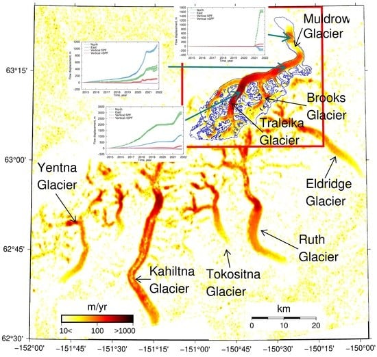
The magnitude of surface velocities for the entire region covered by the ascending and descending SAR data is shown in Figure 3. There, we use a logarithmic scale to visualize the full range of the magnitude without oversaturation. In Figure 4 we focus on the Muldrow Glacier and its tributaries and use a SAR intensity image in the background for reference. The Structure-from-Motion (SfM)-derived dem acquired on 20210919 is shown in Figure 4a, the magnitude of horizontal flow velocity is shown in Figure 4b, and the vertical SPF and nSPF flow velocities are shown in Figure 4c,d. From 2014–2021, flow velocities at the Muldrow Glacier vary significantly, which cannot be captured in one figure. Therefore, for describing temporal variability at the Mudrow Glacier, we sample along the central flowline. This flowline is derived from the output of the Open Global Glacier Model (OGGM) software [8]. It is computed in an easily reproducible way but it only approximately follows the actual flowlines of the glacier. For the 5 × 5-pixel regions, located on the central flowline at 5 km intervals, at distances 5–40 km in the direction of flow, we also show time series. In these regions, 25-pixel sample standard deviation is computed and shown in the figures. It is important to note that this standard deviation is not an accurate measurement of errors since it underestimates long-wavelength signals and overestimates short-wavelength signals.
For validating our results, we compute the magnitudes of horizontal flow velocities during the 2017 and 2018 periods by differencing the cumulative flow displacements at the beginning and the end of respective epochs and dividing them by the timespan of one year. These results then are compared with the results presented in Gardner et al. [9] (Figure 5). There, surface velocities are derived from Landsat 4, 5, 7, and 8 imagery over the respective periods using the auto-RIFT feature tacking processing chain described in Gardner et al. [10]. Overall the results are in a reasonable agreement, even that Landsat-derived measurements capture velocities at the surface, and SAR-derived measurements capture velocities at some depth that depends on the dielectric properties of ice. Flow velocities decrease with depth due to friction between the glacier’s ice and its bed. During the 2017 period, the correlation coefficient between the SAR-derived and Landsat-derived magnitudes of horizontal velocities is 0.91, and the root-mean-square error is 70 m/year. During the 2018 period, the correlation coefficient is 0.82, and the root-mean-square error is 122 m/year.
The time series of horizontal and vertical velocities along the central flowlines are shown in Figure 6. From the beginning of observation until the end of 2018, a region of fast horizontal velocity (surge) propagates from the glacier’s head to its central part (8–18 km segment of the central flowline). Then in 2019, the surge propagates further down (22–30 km segment), and in 2020 a large part of the glacier (segment 10–35 km) surges with even larger velocities. The 2020 surge starts at the central part of the glacier (22–34 km segment) and then propagates in both directions, upward and downward. Finally, starting in late 2020 and during 2021, the surge reaches the glacier’s terminus (38–43 km segment), and at the same time, two new smaller surges occur near the glacier’s head (5 and 10 km segments).
During the entire observation period, the vertical nSPF component shows predominantly upward motion (Figure 6b), with an exception during 2020, when downward motion is observed in the upper 35 km part of the glacier. The positive values of vertical nSPF velocity signify a mass transfer from high elevation to low elevation, which is expected during the surge. The time series of flow velocities (Figure 7) and flow displacements (Figure 8) show another perspective of surge evolution. For example, they show that an increase in flow velocity starts in the upper part of the glacier as early as 2017 and then propagates downward, and it is not uniform in time and space.
An animation that shows the dynamics of the flow velocity field along the central flowline is provided in the Supplementary Materials [11]. The presented results fully describe the flow velocity of a glacier that can be deduced from a single SAR sensor.
4. Discussion and Conclusions
Availability of a regularity acquired on ascending and descending orbits Sentinel-1 SAR data provides an opportunity for studying the time-dependent dynamics of glaciers. We analyze glacier flow at the Mudrow Glacier, located in the Denali National Park and Preserve (Alaska, AK, USA), using Sentinel-1 SAR data acquired from October 2014 to November 2021. For computing the individual components of flow velocity we apply the MSBAS-4D technique, which produces north, east, and vertical SPF and nSPF components of flow velocities and displacements. The vertical SPF component assumes motion parallel to the glacier bed and thus reflects vertical changes in ice flow due to the advection of ice along the surface. The nSPF component is driven by variations in mass balance and residual changes in surface elevation. We validate the horizontal velocities during the 2017 and 2018 periods using Landsat-derived data. We observe seasonal fluctuation in the vertical nSPF velocity. Such signal is previously observed at other glaciers in southern Alaska and Yukon, which provides an additional validation.
For computing average flow velocities over the entire seven years period (Figure 3 and Figure 4) we apply linear regression to flow displacement time series, which also produces standard deviations and coefficients of determination for each component. From the timeseries computed along the central flowline, and in more detail at eight regions located on that central flowline, it is apparent that the velocity is not constant and that the linear model cannot adequately capture all the information stored in the time series. Nevertheless, average velocities are still used here but only to demonstrate the overall flow trend. The instantaneous velocities for each map pixel can be extracted from the data provided in the supplement and aggregated to produce velocities over any specific intervals (e.g., monthly, quarterly).
The complexity of a surge at this remote glacier is mapped with the 9-day spatial resolution and 100 m grid spacing. The initial increase in the glacier flow velocities is observed starting as early as 2017. The fastest increase is observed in 2020, it reaches the glacier terminus in 2021. Smaller surges are also observed in 2021 in the upper and middle parts of the glacier and their progress is yet unknown.
This fully-automated processing system presented here has been developed at the Canada Centre for Remote Sensing to support the processing of SAR data from the RADARSAT Constellation Mission (RCM) satellites launched on 12 June 2019 [12,13,14]. It can, however, process SAR data from many sensors, including Sentinel-1. Presently, we share with the research community only one component of the system, the MSBAS software that computes time series from individual range/azimuth speckle offset maps. Speckle offset-derived time series is conceptually identical to Differential Interferometric SAR (DInSAR)-derived time series; however, the magnitude of the displacements over a typical 12-day interval is significantly greater, sometimes exceeding multiple SAR pixels. SAR-derived time series are routinely compared to Global Navigation Satellite System (GNSS)-derived time series. However, GNSS-derived measurements assume Lagrangian representation but the representation of SAR-derived measurements is more complex than previously thought [6], neither purely Lagrangian, nor Eulerian, and which deserves additional investigation.
Figure 1.
Study region is located in Denali National Park and Preserve of Interior Alaska. Footprints of Sentinel-1 ascending and descending swaths, used in this study, are outlined in black. Area of Interest (AOI) shows location of Muldrow Glacier, which is outlined in blue. Background is Advanced Spaceborne Thermal Emission and Reflection Radiometer (ASTER) digital elevation model (DEM) [15] with a spatial resolution of 30 m. Insert in top-left corner shows the location of the study region in North America.

Figure 2.
Spatial and temporal baselines of Sentinel-1 ascending track 065 (a) and descending track 131 pairs (b) used in this study. Mean temporal resolution, i.e., mean temporal spacing between consecutive SAR acquisitions regardless of orbit direction, computed as duration divided by number of SAR images minus one is about 9 days. Note that offset between perpendicular baselines of ascending and descending sets depends on selection of reference images, which is arbitrary.

Figure 3.
Magnitude of mean 4D flow velocities during 20141026–2021118, computed from Sentinel-1 ascending/descending range/azimuth offsets and plotted using logarithmic scale. Outline and names of glaciers are from Global Land Ice Measurements from Space database [16].
Figure 3.
Magnitude of mean 4D flow velocities during 20141026–2021118, computed from Sentinel-1 ascending/descending range/azimuth offsets and plotted using logarithmic scale. Outline and names of glaciers are from Global Land Ice Measurements from Space database [16].

Figure 4.
(a) SfM-derived DEM acquired on 20210919, (b) magnitude of flow velocity in horizontal direction and flow velocity in (c) vertical SPF and (d) vertical nSPF directions during 20141026–20211108. Background is intensity of Sentinel-1 image acquired on 20210907. Central flowline in green is derived from output of Open Global Glacier Model (OGGM) software [8]. Markers in green show distance along central flowline in km, for which time series are shown in Figure 7 and Figure 8.

Figure 5.
Comparison between SAR-derived (this study) and Landsat-derived [9,10] magnitude of mean horizontal flow velocities during year (a) 2017 and (b) 2018. For these tests only, SAR-derived flow velocity was computed as flow displacement over respectful periods divided by time interval of one year.

Figure 6.
Temporal evolution of (a) magnitude of horizontal flow velocity and (b) vertical nSPF flow velocity during 20141026–20211108.
Figure 6.
Temporal evolution of (a) magnitude of horizontal flow velocity and (b) vertical nSPF flow velocity during 20141026–20211108.

Figure 7.
4D flow velocity time series for (a) 5, (b) 10, (c) 15, (d) 20, (e) 25, (f) 30, (g) 35, (h) 40 km markers along central flowline of Muldrow Glacier.
Figure 7.
4D flow velocity time series for (a) 5, (b) 10, (c) 15, (d) 20, (e) 25, (f) 30, (g) 35, (h) 40 km markers along central flowline of Muldrow Glacier.

Figure 8.
4D flow displacement time series for (a) 5, (b) 10, (c) 15, (d) 20, (e) 25, (f) 30, (g) 35, (h) 40 km markers along central flowline of Muldrow Glacier.
Figure 8.
4D flow displacement time series for (a) 5, (b) 10, (c) 15, (d) 20, (e) 25, (f) 30, (g) 35, (h) 40 km markers along central flowline of Muldrow Glacier.

One of the biggest challenges in processing SAR data over glaciers is the potentially low quality of the computed range/azimuth offset maps. It usually happens when a glacier melts or when it experiences fast flow. To overcome this problem, MSBAS is designed to work with range/azimuth offset maps that have partial spatial coverage, assuming that low-quality regions in the individual range/azimuth offset maps are removed. The reliability of produced time series is measured at each pixel by a rank of the time matrix [5], and a user can remove pixels that have a low rank in post-processing. Therefore, optimal processing parameters, such as a rank threshold, can be tested without the need to reprocess data, which is a processing power-intensive and time-consuming operation.
The quality of the individual range/azimuth offset maps produced with GAMMA software depends on selected processing parameters, especially the size of the range/azimuth correlation window. On one hand, we want to select a large window to get a statistically significant peak of the 2D cross-correlation function. On the other hand, a large window decreases the spatial resolution of the computed offset maps (not to be mistaken with spatial grid spacing that can be chosen arbitrarily). The same applies to the size and strength of the spatial filter, which should be large enough (in comparison with the glacier size, especially its width and the smoothness of the velocity field) to reduce noise but not too large to preserve the desired spatial resolution. We tested the processing parameters used in this study on several glaciers (e.g., [5,6]) in a fully-automated processing regime when prior knowledge about the region and the velocity field is not available. These parameters may be suboptimal in specific circumstances, for example, when the flow velocity or velocity gradient is large or when the width of a glacier is small.
We expect that the fully-automated processing systems, similar to the one presented here, will play an increasingly dominant role and soon entirely replace manual processing. From our experience, the large cost of high-performance storage capable of supporting parallel processing of large data sets is a bottleneck of the current processing system. Therefore, we pay particular attention to removing intermediate products as soon as they become no longer needed in the following processing. Systems designed to process big satellite data must value every bit of a processing resource because the ever-increasing availability of SAR data regularly redefines the meaning of big in big satellite data.
Supplementary Materials
The supporting information [11] can be downloaded at: https://0-doi-org.brum.beds.ac.uk/10.17632/8d7pjd7f86.1.
Funding
This work has been supported by the Canadian Centre for Remote Sensing, NRCan under the Status and Trend Mapping Program.
Data Availability Statement
Sentinel-1 Single Look Complex images used in this study can be downloaded from the Alaska Satellite Facility at https://asf.alaska.edu. Computed flow displacement and flow velocity products and an annimation can be downloaded from Mendeley Data at https://0-doi-org.brum.beds.ac.uk/10.17632/8d7pjd7f86.1.
Acknowledgments
We thank the European Space Agency for acquiring, and the National Aeronautics and Space Administration (NASA) and Alaska Satellite Facility (ASF) for distributing Sentinel-1 SAR data. Figures were plotted with GMT 6.0.0 and Gnuplot 5.2 software. NRCan contribution number/Numéro de contribution de RNCan: 20220091. We especially thank Chad Hults from the National Park Service in Anchorage, AK, for providing SfM-derived DEMs and other supporting data that helped us understand better the surge dynamics at this glacier.
Conflicts of Interest
The authors declare no conflict of interest.
References
- Meier, M.F.; Post, A. What are glacier surges? Can. J. Earth Sci. 1969, 6, 807–817. [Google Scholar] [CrossRef]
- Post, A.S. The exceptional advances of the Muldrow, Black Rapids, and Susitna glaciers. J. Geophys. Res. 1960, 65, 3703–3712. [Google Scholar] [CrossRef]
- Harrison, A.E. Ice Surges on the Muldrow Glacier, Alaska. J. Glaciol. 1964, 5, 365–368. [Google Scholar] [CrossRef] [Green Version]
- Harrison, A.E. Glacial activity preceding the 1956 Muldrow Glacier surge in Alaska. Can. J. Earth Sci. 1969, 6, 1001–1007. [Google Scholar] [CrossRef]
- Samsonov, S.; Tiampo, K.; Cassotto, R. Measuring the state and temporal evolution of glaciers in Alaska and Yukon using synthetic-aperture-radar-derived (SAR-derived) 3D time series of glacier surface flow. Cryosphere 2021, 15, 4221–4239. [Google Scholar] [CrossRef]
- Samsonov, S.; Tiampo, K.; Cassotto, R. SAR-derived flow velocity and its link to glacier surface elevation change and mass balance. Remote Sens. Environ. 2021, 258, 112343. [Google Scholar] [CrossRef]
- Wegmuller, U.; Werner, C. GAMMA SAR processor and interferometry software. In Proceedings of the 3rd ERS Symposium on Space at the Service of Our Environment, Florence, Italy, 14–21 March 1997. [Google Scholar]
- Maussion, F.; Butenko, A.; Champollion, N.; Dusch, M.; Eis, J.; Fourteau, K.; Gregor, P.; Jarosch, A.H.; Landmann, J.; Oesterle, F.; et al. The Open Global Glacier Model (OGGM) v1.1. Geosci. Model Dev. 2019, 12, 909–931. [Google Scholar] [CrossRef] [Green Version]
- Gardner, A.; Fahnestock, M.; Scambos, T. MEASURES ITS_LIVE Regional Glacier and Ice Sheet Surface Velocities. 2019. Available online: https://nsidc.org/apps/itslive/ (accessed on 1 February 2022). [CrossRef]
- Gardner, A.S.; Moholdt, G.; Scambos, T.; Fahnstock, M.; Ligtenberg, S.; van den Broeke, M.; Nilsson, J. Increased West Antarctic and unchanged East Antarctic ice discharge over the last 7 years. Cryosphere 2018, 12, 521–547. [Google Scholar] [CrossRef] [Green Version]
- Samsonov, S. Data for: Operational Processing of Big Satellite Data for Monitoring Glacier Dynamics. Case Study Muldrow Glacier; Mendeley Data, V1. 2022. Available online: https://data.mendeley.com/datasets/8d7pjd7f86/1 (accessed on 1 February 2022). [CrossRef]
- Dudley, J.P.; Samsonov, S.V. The Government of Canada Automated Processing System for Change Detection and Ground Deformation Analysis from RADARSAT-2 and RADARSAT Constellation Mission Synthetic Aperture Radar Data: Description and User Guide; Technical Report; Government of Canada: Moncton, NB, Canada, 2020. [CrossRef]
- Dudley, J.P.; Samsonov, S.V. Système de Traitement Automatisé du Gouvernement Canadien Pour la Détection des Variations et L’analyse des Déformations du sol à Partir des Données de Radar à Synthèse D’ouverture de RADARSAT-2 et de la Mission de la Constellation RADARSAT: Description et Guide de L’utilisateur; Technical Report; Government of Canada: Moncton, NB, Canada, 2021. [CrossRef]
- Dudley, J.P.; Samsonov, S.V. SAR Interferometry with the RADARSAT Constellation Mission; Technical Report; Government of Canada: Moncton, NB, Canada, 2022. [CrossRef]
- Abrams, M.; Crippen, R.; Fujisada, H. ASTER Global Digital Elevation Model (GDEM) and ASTER Global Water Body Dataset (ASTWBD). Remote Sens. 2020, 12, 1156. [Google Scholar] [CrossRef] [Green Version]
- GLIMS Consortium. GLIMS Glacier Database; Version 1; National Snow and Ice Data Center: Boulder, CO, USA, 2005. [Google Scholar] [CrossRef]

Table 1.
Sentinel-1 SAR data used in this study, where is incidence and is azimuth angles, SLC is number of SLC images, and SPO is number of range/azimuth offset products.
Table 1.
Sentinel-1 SAR data used in this study, where is incidence and is azimuth angles, SLC is number of SLC images, and SPO is number of range/azimuth offset products.
| Set | Span | SLC | SPO | ||
|---|---|---|---|---|---|
| Sentinel-1 T065(asc) | 20141022–20211108 | 39 | 341 | 135 | 134 |
| Sentinel-1 T131(dsc) | 20141026–20211118 | 39 | 199 | 164 | 163 |
Publisher’s Note: MDPI stays neutral with regard to jurisdictional claims in published maps and institutional affiliations. |
© 2022 by the author. Licensee MDPI, Basel, Switzerland. This article is an open access article distributed under the terms and conditions of the Creative Commons Attribution (CC BY) license (https://creativecommons.org/licenses/by/4.0/).
Share and Cite
MDPI and ACS Style
Samsonov, S.V. Operational Processing of Big Satellite Data for Monitoring Glacier Dynamics: Case Study of Muldrow Glacier. Remote Sens. 2022, 14, 2679. https://0-doi-org.brum.beds.ac.uk/10.3390/rs14112679
AMA Style
Samsonov SV. Operational Processing of Big Satellite Data for Monitoring Glacier Dynamics: Case Study of Muldrow Glacier. Remote Sensing. 2022; 14(11):2679. https://0-doi-org.brum.beds.ac.uk/10.3390/rs14112679
Chicago/Turabian StyleSamsonov, Sergey V. 2022. "Operational Processing of Big Satellite Data for Monitoring Glacier Dynamics: Case Study of Muldrow Glacier" Remote Sensing 14, no. 11: 2679. https://0-doi-org.brum.beds.ac.uk/10.3390/rs14112679
Note that from the first issue of 2016, this journal uses article numbers instead of page numbers. See further details here.