
On the Reconstruction of Missing Sea Surface Temperature Data from Himawari-8 in Adjacent Waters of Taiwan Using DINEOF Conducted with 25-h Data

 , ,
, ,
Abstract
:1. Introduction
2. Materials and Methods
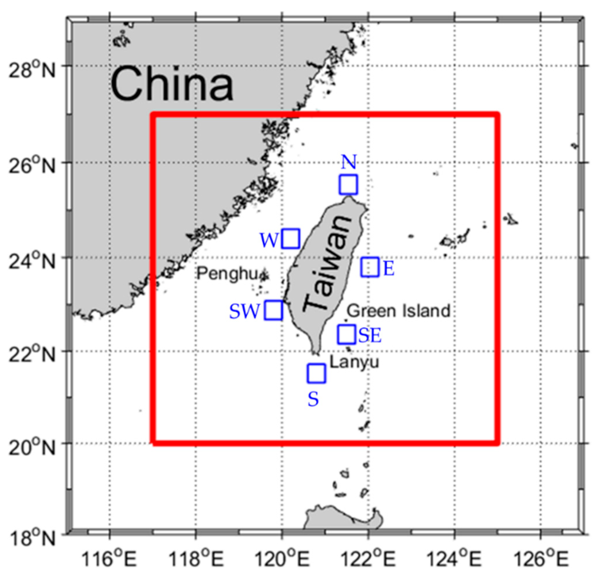
2.1. SST Data
2.2. DINEOF Method
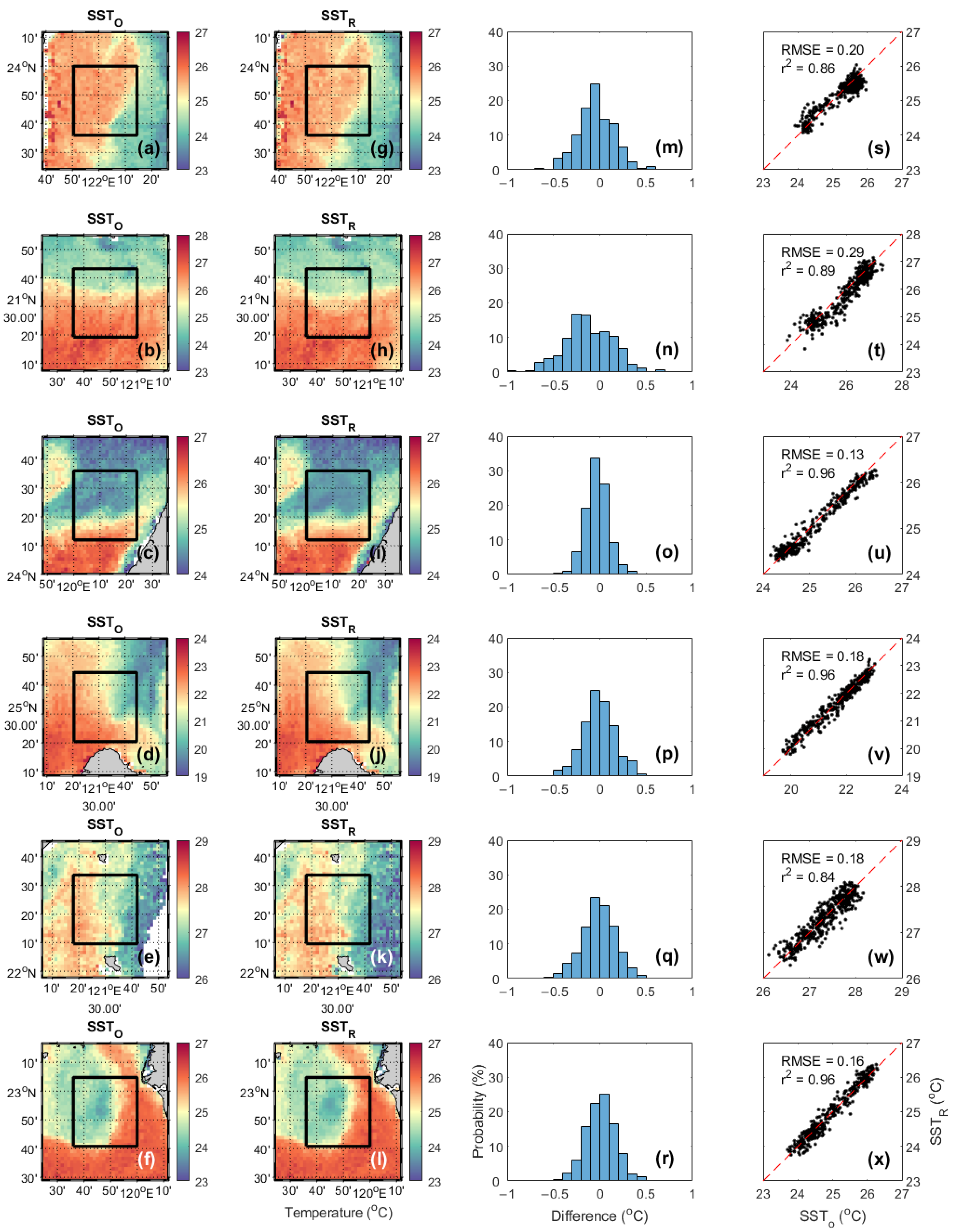
3. Results
3.1. Preliminary Analysis of SST Data
3.2. DINEOF Results
4. Discussion
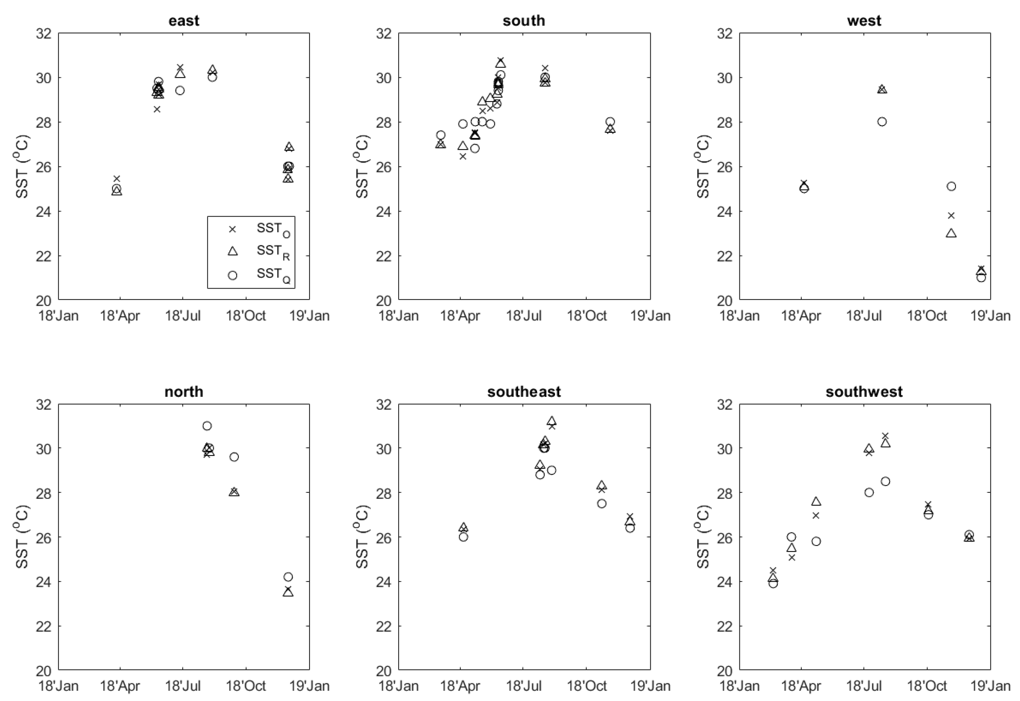
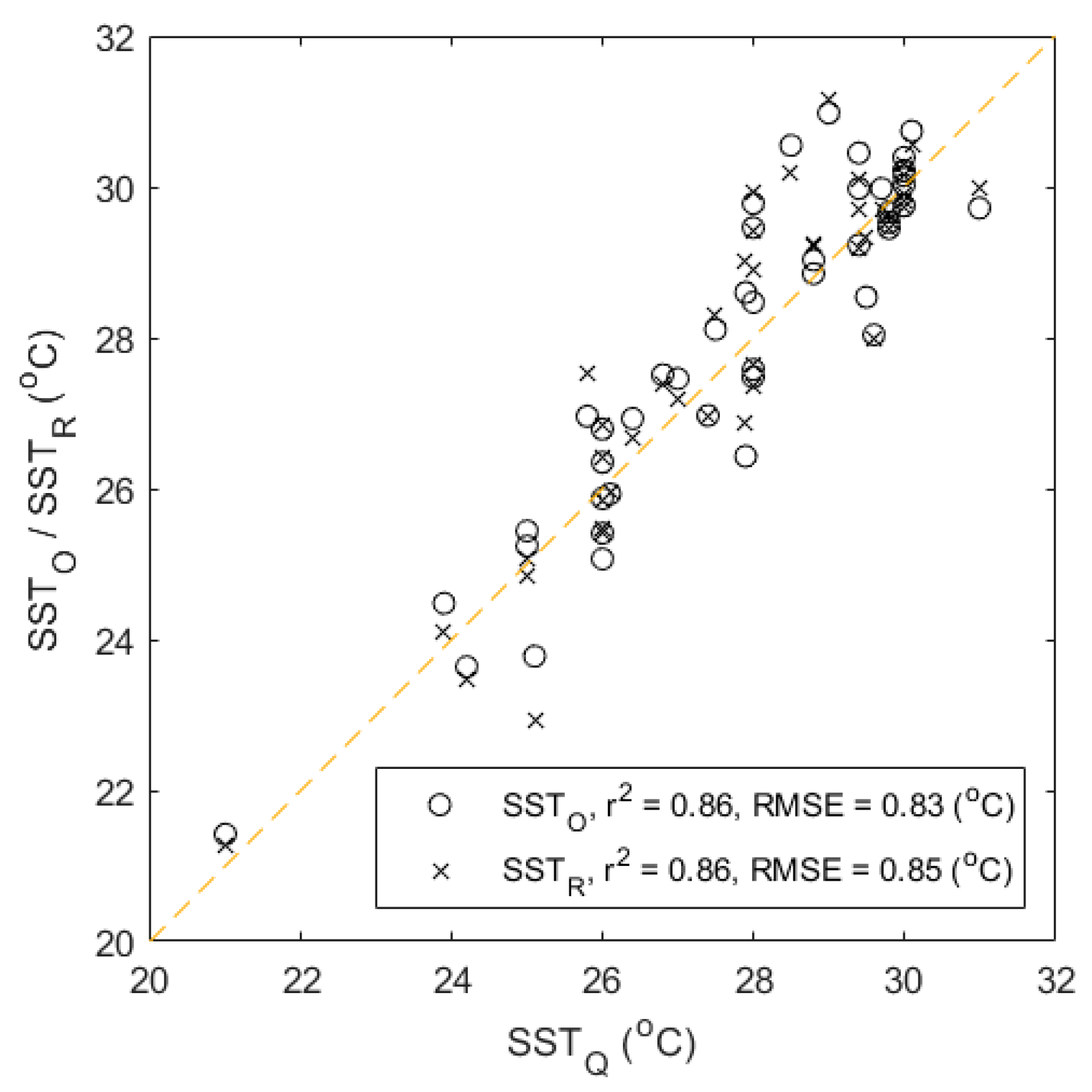
4.1. Comparison of SSTR with Other SST Data
4.1.1. iQuam SST
4.1.2. MODIS SST
4.2. Influence of SST Variations on SSTR
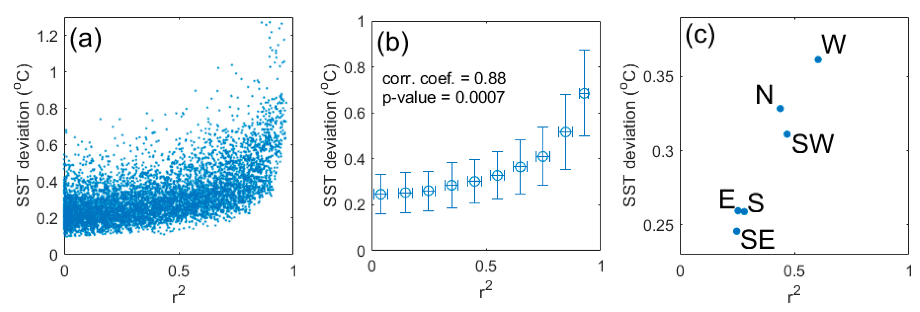
4.3. Influence of Missing Data Rate on SSTR
5. Conclusions
- The DINEOF method is affected by the magnitude of SST variation in the study region. If there are more obvious SST characteristics, that is, higher variation in the region, the results of the reconstruction are better and the RMSE is smaller.
- The missing rate of the original data does not substantially affect the accuracy of the reconstructed data. However, from a statistical point of view, the higher the missing data rate of the original data, the less accurate the reconstructed data may be.
Author Contributions
Funding
Data Availability Statement
Acknowledgments
Conflicts of Interest
References
- IPCC. Climate Change 2021: The Physical Science Basis; Masson-Delmotte, V., Zhai, P., Pirani, A., Connors, S.L., Péan, C., Berger, S., Caud, N., Chen, Y., Goldfarb, L., Gomis, M.I., et al., Eds.; Cambridge University Press: Cambridge, UK, 2021. [Google Scholar]
- Martin, S. An Introduction to Ocean Remote Sensing, 2nd ed.; Cambridge University Press: Cambridge, UK, 2014. [Google Scholar]
- Cochran, J.K.; Bokuniewicz, H.J.; Yager, P.L. Encyclopedia of Ocean Sciences, 3rd ed.; Elsevier Science: Amsterdam, The Netherlands, 2019. [Google Scholar]
- Wallace, J.M.; Dickison, R.E. Empirical orthogonal representation of time series in the frequency domain. Part I: Theoretical considerations. J. Appl. Meteorol. Climatol. 1972, 11, 887–892. [Google Scholar] [CrossRef]
- Beckers, J.M.; Rixen, M. EOF calculations and data filling from incomplete oceanographic datasets. J. Atmos. Ocean. Technol. 2003, 20, 1839–1856. [Google Scholar] [CrossRef]
- Alvera-Azcárate, A.; Barth, A.; Rixen, M.; Beckers, J.M. Reconstruction of incomplete oceanographic data sets using empirical orthogonal functions: Application to the Adriatic Sea surface temperature. Ocean Model. 2005, 9, 325–346. [Google Scholar] [CrossRef] [Green Version]
- Daley, R. Atmospheric Data Analysis; Cambridge University Press: Cambridge, UK, 1991. [Google Scholar]
- Beckers, J.M.; Barth, A.; Alvera-Azcárate, A. DINEOF reconstruction of clouded images including error maps-application to the Sea-Surface Temperature around Corsican Island. Ocean Sci. 2006, 2, 183–199. [Google Scholar] [CrossRef] [Green Version]
- Elken, J.; Zujev, M.; She, J.; Lagemaa, P. Reconstruction of large-scale sea surface temperature and salinity fields using sub-regional EOF patterns from models. Front. Earth Sci. 2019, 7, 232. [Google Scholar] [CrossRef] [Green Version]
- Alvera-Azcárate, A.; Barth, A.; Beckers, J.M.; Weisberg, R.H. Multivariate reconstruction of missing data in sea surface temperature, chlorophyll, and wind satellite fields. J. Geophys. Res. 2007, 112, C03008. [Google Scholar]
- Hsu, P.C.; Lu, C.Y.; Hsu, T.W.; Ho, C.R. Diurnal to seasonal variations in ocean chlorophyll and ocean currents in the north of Taiwan observed by Geostationary Ocean Color Imager and coastal radar. Remote Sens. 2020, 12, 2853. [Google Scholar] [CrossRef]
- Jan, S.; Chern, C.S.; Wang, J.; Chao, S.Y. The anomalous amplification of M2 tide in the Taiwan Strait. Geophys. Res. Lett. 2004, 31, L07308. [Google Scholar] [CrossRef]
- Lan, K.W.; Kawamura, H.; Lee, M.A.; Chang, Y.; Chan, J.W.; Liao, C.H. Summertime sea surface temperature fronts associated with upwelling around the Taiwan Bank. Cont. Shelf Res. 2009, 29, 903–910. [Google Scholar] [CrossRef]
- Chang, M.H.; Jan, S.; Mensah, V.; Andres, M.; Rainville, L.; Yang, Y.J.; Cheng, Y.H. Zonal migration and transport variations of the Kuroshio east of Taiwan induced by eddy impingements. Deep-Sea Res. Part I Oceanogr. Res. Pap. 2018, 131, 1–15. [Google Scholar] [CrossRef]
- Hsu, P.C.; Ho, C.Y.; Lee, H.J.; Lu, C.Y.; Ho, C.R. Temporal variation and spatial structure of the Kuroshio-induced submesoscale island vortices observed from GCOM-C and Himawari-8 data. Remote Sens. 2019, 12, 883. [Google Scholar] [CrossRef] [Green Version]
- Zheng, Q.; Hu, J.Y.; Ho, C.R.; Xie, L.L. Advances in research of regional oceanography of the South China Sea: Overview. In Regional Oceanography of the South China Sea; Hu, J.Y., Ho, C.R., Xie, L.L., Zheng, Q., Eds.; World Scientific: Singapore, 2019; pp. 1–18. [Google Scholar]
- Weare, B.C.; Nasstrom1, J.S. Examples of extended empirical orthogonal function analyses. Mon. Weather Rev. 1982, 110, 481–485. [Google Scholar] [CrossRef]
- Thomson, R.E.; Emery, W.J. Data Analysis Methods in Physical Oceanography, 3rd ed.; Elsevier Science: Amsterdam, The Netherlands, 2014. [Google Scholar]
- Ping, B.; Su, F.; Meng, Y. An improved DINEOF algorithm for filling missing values in spatio-temporal sea surface temperature data. PLoS ONE 2016, 11, 0155928. [Google Scholar] [CrossRef] [Green Version]
- Huynh, H.N.T.; Alvera-Azcárate, A.; Barth, A.; Beckers, J.M. Reconstruction and analysis of long-term satellite-derived sea surface temperature for the South China Sea. J. Oceanogr. 2016, 72, 707–726. [Google Scholar] [CrossRef]
- Central Weather Bureau. Climate Monitoring: 2018 Annual Report. (In Chinese). Available online: https://www.cwb.gov.tw/Data/service/notice/download/publish_20191104141027.pdf (accessed on 27 April 2022).
- Grodsky, S.A.; Bentamy, A.; Carton, J.A.; Pinker, R.T. Intraseasonal latent heat flux based on satellite observations. J. Clim. 2009, 22, 4539–4556. [Google Scholar] [CrossRef] [Green Version]
- Rex, X.; Yang, X.-Q.; Hu, H. Subseasonal variations of wintertime North Pacific evaporation, cold air surges, and water vapor transport. J. Clim. 2017, 30, 9475–9491. [Google Scholar]
- Xu, F.; Ignatov, A. In situ SST quality monitor (iQuam). J. Atmos. Ocean. Technol. 2014, 31, 164–180. [Google Scholar] [CrossRef]


| Sea Area | Latitude (°N) | Longitude (°E) | Number of Data |
|---|---|---|---|
| East (E) | 121.84–122.24 | 23.6–24.0 | 738 |
| South (S) | 120.6–121.0 | 21.32–21.72 | 1141 |
| West (W) | 120.0–120.4 | 24.2–24.6 | 1359 |
| North (N) | 121.34–121.74 | 25.34–25.74 | 1116 |
| Southeast (SE) | 121.30–121.70 | 22.16–22.56 | 1065 |
| Southwest (SW) | 119.6–120.0 | 22.68–23.08 | 1480 |
| Sea Area | Number of Matching Points | SSTQ with SSTR | SSTQ with SSTO | ||||
|---|---|---|---|---|---|---|---|
| RMSE (°C) | r2 | p-Value | RMSE (°C) | r2 | p-Value | ||
| East (E) | 10 | 0.44 | 0.95 | <0.001 | 0.58 | 0.91 | <0.001 |
| South (S) | 14 | 0.58 | 0.77 | <0.001 | 0.60 | 0.80 | <0.001 |
| West (W) | 4 | 1.29 | 0.83 | 0.0895 | 1.01 | 0.89 | 0.0546 |
| North (N) | 4 | 1.02 | 0.96 | 0.0187 | 1.05 | 0.94 | 0.0279 |
| Southeast (SE) | 7 | 0.91 | 0.86 | 0.0029 | 0.83 | 0.87 | 0.0022 |
| Southwest (SW) | 7 | 1.19 | 0.85 | 0.0029 | 1.20 | 0.85 | 0.0030 |
| Sea Area | Terra Daytime SSTM | Terra Nighttime SSTM | Aqua Daytime SSTM | Aqua Nighttime SSTM | ||||||||||||
|---|---|---|---|---|---|---|---|---|---|---|---|---|---|---|---|---|
| SSTR | SSTO | SSTR | SSTO | SSTR | SSTO | SSTR | SSTO | |||||||||
| RMSE | r2 | RMSE | r2 | RMSE | r2 | RMSE | r2 | RMSE | r2 | RMSE | r2 | RMSE | r2 | RMSE | r2 | |
| E | 0.79 | 0.88 | 0.73 | 0.91 | 0.63 | 0.92 | 0.69 | 0.91 | 0.78 | 0.85 | 0.78 | 0.86 | 0.59 | 0.91 | 0.55 | 0.92 |
| S | 0.67 | 0.83 | 0.63 | 0.86 | 0.65 | 0.74 | 0.63 | 0.76 | 0.68 | 0.82 | 0.68 | 0.82 | 0.84 | 0.67 | 0.85 | 0.69 |
| W | 0.69 | 0.95 | 0.68 | 0.95 | 0.58 | 0.94 | 0.55 | 0.95 | 0.67 | 0.93 | 0.67 | 0.93 | 0.67 | 0.94 | 0.64 | 0.95 |
| N | 0.59 | 0.97 | 0.60 | 0.97 | 0.67 | 0.93 | 0.67 | 0.93 | 0.78 | 0.95 | 0.75 | 0.96 | 0.65 | 0.94 | 0.62 | 0.94 |
| SE | 0.76 | 0.86 | 0.74 | 0.86 | 0.72 | 0.81 | 0.73 | 0.81 | 0.67 | 0.86 | 0.66 | 0.86 | 0.69 | 0.80 | 0.69 | 0.80 |
| SW | 0.79 | 0.87 | 0.71 | 0.90 | 0.76 | 0.82 | 0.73 | 0.84 | 0.67 | 0.92 | 0.65 | 0.92 | 0.74 | 0.85 | 0.73 | 0.86 |
Publisher’s Note: MDPI stays neutral with regard to jurisdictional claims in published maps and institutional affiliations. |
© 2022 by the authors. Licensee MDPI, Basel, Switzerland. This article is an open access article distributed under the terms and conditions of the Creative Commons Attribution (CC BY) license (https://creativecommons.org/licenses/by/4.0/).
Share and Cite
Yang, Y.-C.; Lu, C.-Y.; Huang, S.-J.; Yang, T.-Z.; Chang, Y.-C.; Ho, C.-R. On the Reconstruction of Missing Sea Surface Temperature Data from Himawari-8 in Adjacent Waters of Taiwan Using DINEOF Conducted with 25-h Data. Remote Sens. 2022, 14, 2818. https://0-doi-org.brum.beds.ac.uk/10.3390/rs14122818
Yang Y-C, Lu C-Y, Huang S-J, Yang T-Z, Chang Y-C, Ho C-R. On the Reconstruction of Missing Sea Surface Temperature Data from Himawari-8 in Adjacent Waters of Taiwan Using DINEOF Conducted with 25-h Data. Remote Sensing. 2022; 14(12):2818. https://0-doi-org.brum.beds.ac.uk/10.3390/rs14122818
Chicago/Turabian StyleYang, Yi-Chung, Ching-Yuan Lu, Shih-Jen Huang, Thwong-Zong Yang, Yu-Cheng Chang, and Chung-Ru Ho. 2022. "On the Reconstruction of Missing Sea Surface Temperature Data from Himawari-8 in Adjacent Waters of Taiwan Using DINEOF Conducted with 25-h Data" Remote Sensing 14, no. 12: 2818. https://0-doi-org.brum.beds.ac.uk/10.3390/rs14122818