
Unified Land–Ocean Quasi-Geoid Computation from Heterogeneous Data Sets Based on Radial Basis Functions


College of Surveying and Geo-Informatics, Tongji University, 1239 Siping Road, Shanghai 200092, China
*
Author to whom correspondence should be addressed.
Remote Sens. 2022, 14(13), 3015; https://0-doi-org.brum.beds.ac.uk/10.3390/rs14133015
Submission received: 16 May 2022
/
Revised: 17 June 2022
/
Accepted: 21 June 2022
/
Published: 23 June 2022
(This article belongs to the Special Issue Space-Geodetic Techniques)
Abstract
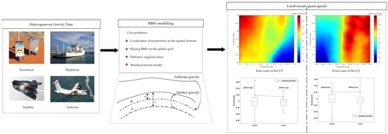
:The determination of the land geoid and the marine geoid involves different data sets and calculation strategies. It is a hot issue at present to construct the unified land–ocean quasi-geoid by fusing multi-source data in coastal areas, which is of great significance to the construction of land–ocean integration. Classical geoid integral algorithms such as the Stokes theory find it difficult to deal with heterogeneous gravity signals, so scholars have gradually begun using radial basis functions (RBFs) to fuse multi-source data. This article designs a multi-layer RBF network to construct the unified land–ocean quasi-geoid fusing measured terrestrial, shipborne, satellite altimetry and airborne gravity data based on the Remove–Compute–Restore (RCR) technique. EIGEN-6C4 of degree 2190 is used as a reference gravity field. Several core problems in the process of RBF modeling are studied in depth: (1) the behavior of RBFs in the spatial domain; (2) the locations of RBFs; (3) ill-conditioned problems of the design matrix; (4) the effect of terrain masses. The local quasi-geoid with a 1′ resolution is calculated, respectively, on the flat east coast and the rugged west coast of the United States. The results show that the accuracy of the quasi-geoid computed by fusing four types of gravity data in the east coast experimental area is 1.9 cm inland and 1.3 cm on coast after internal verification (the standard deviation of the quasi-geoid w.r.t GPS/leveling data). The accuracy of the quasi-geoid calculated in the west coast experimental area is 2.2 cm inland and 2.1 cm on coast. The results indicate that using RBFs to calculate the unified land–ocean quasi-geoid from heterogeneous data sets has important application value.
1. Introduction
The geoid is a fundamental element in determining the shape of the Earth [1]. The calculation of a high-quality geoid requires firstly constructing the Earth’s gravity field with high precision and resolution. With the enrichment of measurement means, the breadth and depth of geospatial data are being continuously improved by terrestrial, shipborne, airborne and satellite gravity surveys, etc. [2,3,4,5,6,7]. The unified land–ocean quasi-geoid can be constructed by fusing heterogeneous data sets in the boundary areas between land and ocean, which is beneficial to advance the construction of land–ocean integration. At present, calculation methods of the gravimetric geoid are mainly divided into analytical methods and statistical methods. Analytical methods include the classical Stokes, Hotine, Molodensky and Helmert integral algorithms [8,9,10,11,12]. The defects of analytical methods lie in the strict requirement of the boundary surface and the difficulty fusing multi-source gravity signals. Statistical methods represented by the least-squares collocation (LSC) have significant advantages in fusing heterogeneous data sets. LSC is first introduced into the study of local gravity field approximation by Krarup and Moritz. Tscherning, Rapp, Hwang and other scholars have performed a lot of later research [13,14,15,16,17]. The defect of LSC is that it is difficult to construct an appropriate and accurate local covariance model. However, as a statistical algorithm, LSC is still a good choice. This article mainly focuses on analytical methods.
Radial basis functions have been widely used in local gravity field modeling in recent years due to their simple function forms and the ability to fuse multi-source data. RBFs are first proposed as a function approximation theory in mathematics [18]. The Multi-quadric (MQ) kernel function proposed by Hardy and the point mass function are first introduced into Earth’s gravity field approximation [19]. Weightman is one of the first scholars to apply the point mass function in physical geodesy. This new method can replace the classical spherical harmonic function to express the Earth’s gravity field. Reilly and Herbrechtsmeier apply the point mass model to the fusion of multi-source data earlier. They use simulated altimetry data to invert marine gravity anomalies and combine the measured gravity anomalies on land to construct a unified local gravity field, whose accuracy reaches 20 mGal after being verified [20]. Barthelmes designs a free-positioned point mass optimization algorithm based on the least-squares adjustment by setting four free parameters on each mass point, which effectively reduces the number of mass points and significantly improves the calculation efficiency [21]. Lehmann further studies the free-positioned algorithm, which can be used more flexibly to determine the local geoid with measured gravity data [22]. These studies lay the foundation of radial basis function modeling. Then, a series of high-order RBFs such as radial multipoles and Poisson wavelets are derived from the point mass function [23,24]. In addition, some scholars introduce the classical Blackman kernel, the Shannon kernel and the spherical spline function into the RBF model [25,26]. After years of development, scholars have performed a lot of research on the application of various RBFs in local gravity field modeling. The research contents mainly focus on the selection of RBF types, the treatment of ill-conditioned problems and the determination of the spatial position of RBFs.
Tenzer and Klees carry out experiments in the plain area to compare the performance of the point mass kernel, the Poisson kernel, radial multipoles and Poisson wavelets. According to the results, they conclude that these RBFs can obtain almost the same accuracy of gravity field modeling when the depth of RBFs is chosen properly [27]. Bentel et al. use simulated data to model the local gravity field based on the Shannon low-pass kernel, the Shannon high-pass kernel, the Blackman low-pass kernel, the cubic polynomial kernel, the Poisson multipoles kernel, the Abel–Poisson kernel truncated and the Abel–Poisson kernel. The experimental results show that the Blackman low-pass kernel, the cubic polynomial kernel and the Abel–Poisson kernel truncated perform best [28]. In the process of RBF modeling, the design matrix may be ill conditioned due to the uneven distribution of observations and excessive number of RBFs. Tikhonov regularization is currently the mainstream method to deal with ill-conditioned problems. Wu et al. adopt zero-order and first-order Tikhonov regularization to solve ill-posed equations and prove that first-order regularization has better performance [29]. Based on the Tikhonov regularization, Liu et al. analyze the defects of the L-curve method and variance component estimation (VCE) in determining regularization parameters and then propose two combined methods, VCE-Lc and Lc-VCE, which are proven to be superior to traditional methods [30,31]. The spatial positions of RBFs have a great influence on the modeling result. Eicker uses various spherical grids to place RBFs such as the Reuter grid, the Triangle-Center grid and the Triangle-Vertex grid, which are more evenly distributed than the geographical grid [32]. Klees and Witter propose an adaptive selection of RBFs before parameter estimation according to the distribution, signal variation and noise of observations [33]. Tenzer and Klees, respectively, use the GCV and RMS minimization methods to determine the optimal depth of RBFs and establish a linear functional relationship between the depth and the correlation length of RBFs. Experiment results prove that the optimal depth is related to the type of RBFs [27]. Tenzer et al. subsequently find in the study of mountainous areas that the RBF model solution is very sensitive to change in depth of even several hundred meters when regional shape fluctuation and gravity signals vary greatly [34]. To sum up the current research by scholars, the main problems are as follows: (1) the selection of RBF types and the determination of spatial positions have not been standardized, which needs further research; (2) the studies carried out using real gravity data and the experiments carried out in the land–ocean boundary areas are still too few.
Considering the above problems, we propose a multi-layer RBF model to fuse heterogeneous data sets for the unified land–ocean quasi-geoid. In Section 2, two coastal areas and relevant experiment data are detailed. The modeling workflow is given, and the modeling methodologies are introduced in detail, including (1) the characteristics of RBFs in the spatial domain; (2) the spatial position of RBFs, i.e., the resolution and depth of spherical grids; (3) Tikhonov regularization to deal with ill-conditioned problems of the model design matrix; (4) residual terrain model (RTM) to represent the impact of terrain mass. The local quasi-geoid with a 1′ resolution is calculated by setting up multi-layer RBF networks, respectively, on the flat east coast and the rugged west coast of the United States in Section 3. In Section 4, we discuss the results and shortcomings of the above research and propose an outlook for future work. Section 5 summarizes the main research content and conclusions of this article.
2. Data and Method
This article studies the RBF model to fuse multi-source gravity data. Numerical experiments are carried out in the land–ocean junction areas. The experiments are conducted in two topographically different areas, one on the east and the other on the west coast of the United States. The east coast of the United States is relatively flat, expending inland from the coastline into a broad plain. On the west coast, under the influence of the Rocky Mountains, the land elevation begins to rise rapidly not far from the coastline. Details of the relevant experiment data are described in this section. In addition, the general modeling process is summarized, and the core modeling methodologies are studied in depth.
2.1. Data Preparation
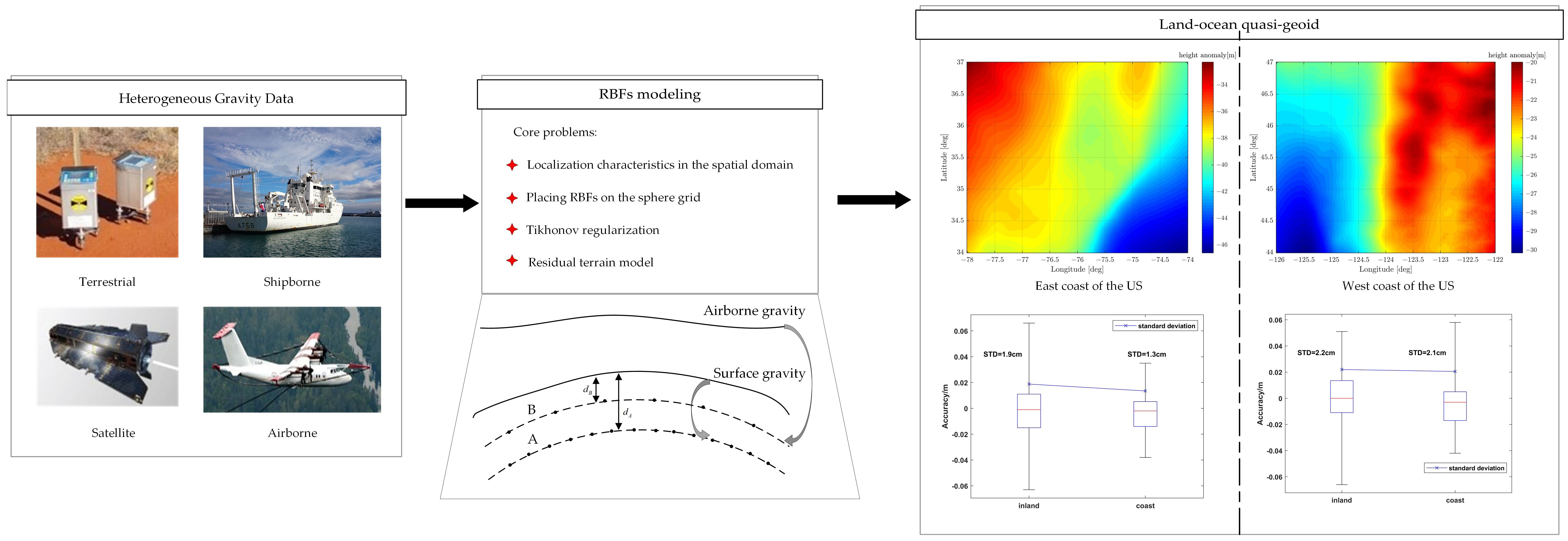
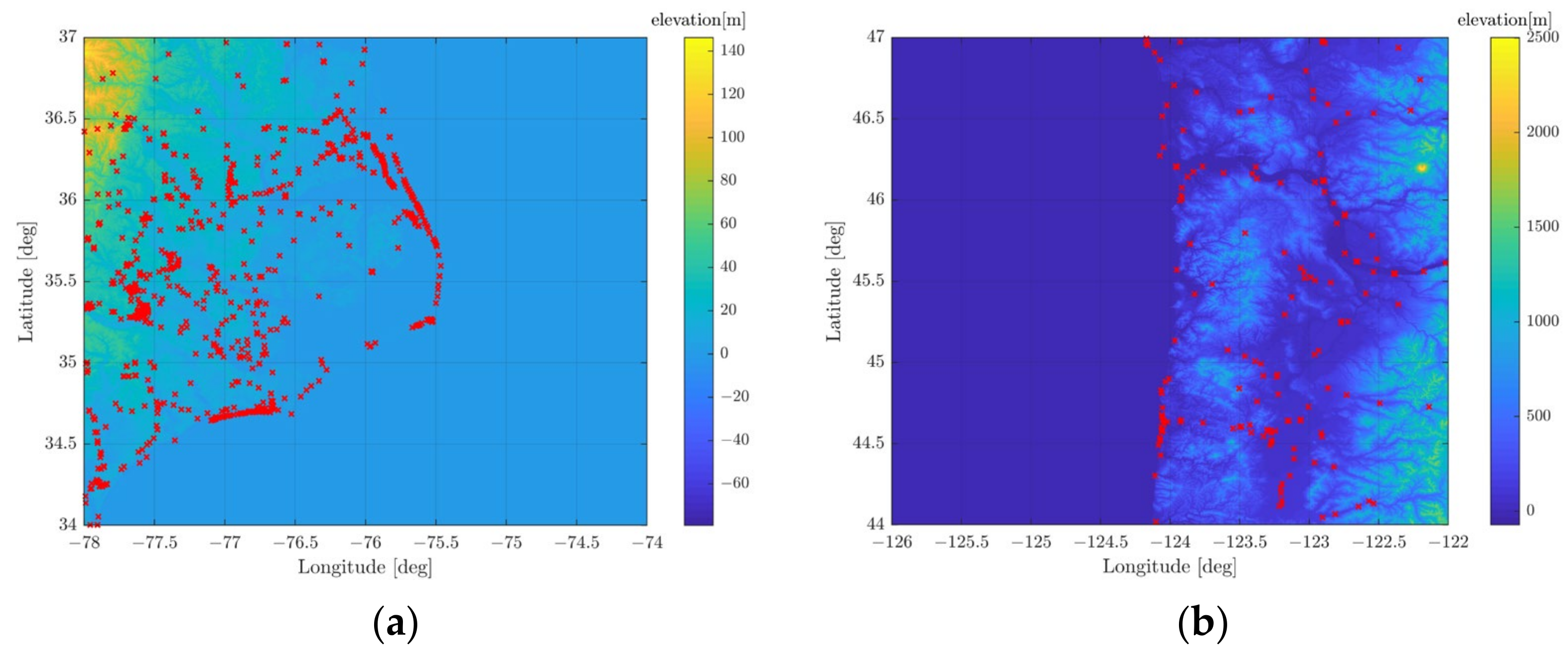
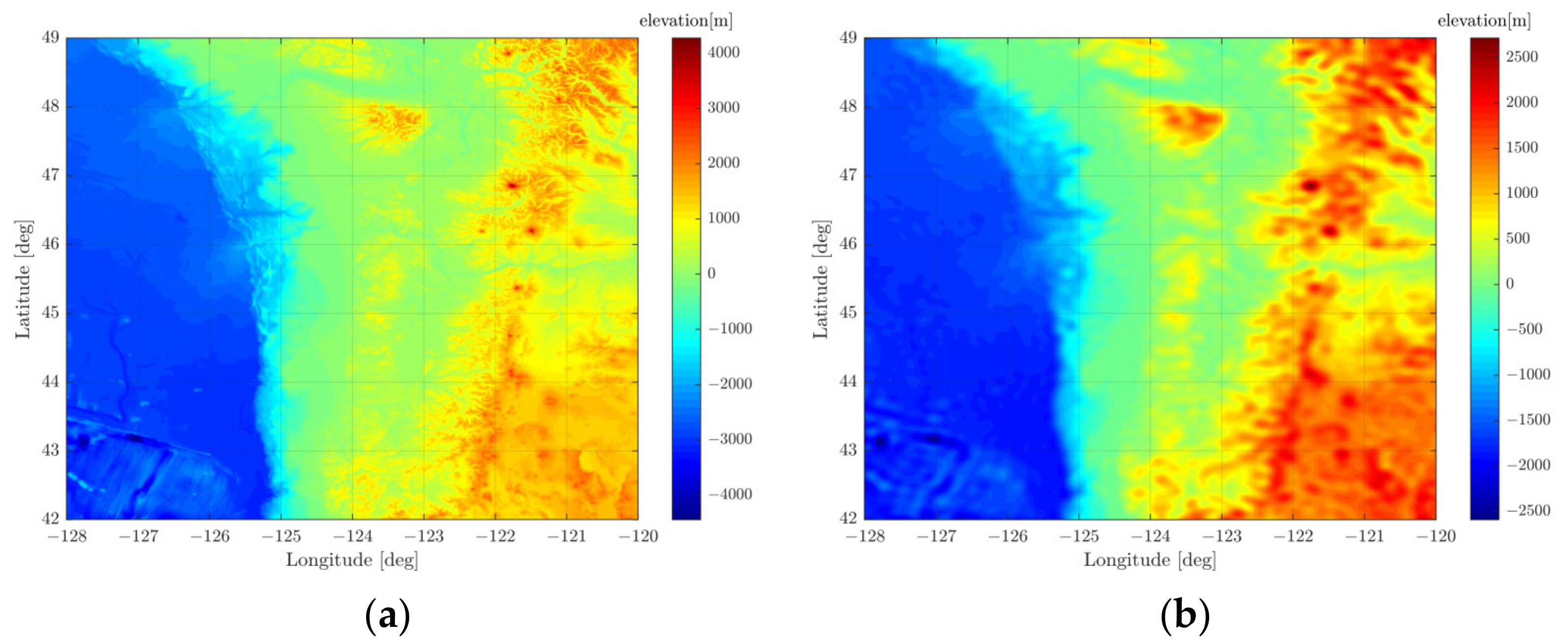
The east coast experiment area is located in North Carolina, USA, with an average elevation of approximately 8 m. The target area range is between 34° and 37° latitude and between −78° and −74° longitude. The west coast experiment area is in the border area of Oregon and Washington State in the northwest of the United States. Its land part is rugged with an average elevation of approximately 334 m. The target area range is between 44° and 47° latitude and between −126° and −122° longitude. The regional topography is shown in Figure 1.
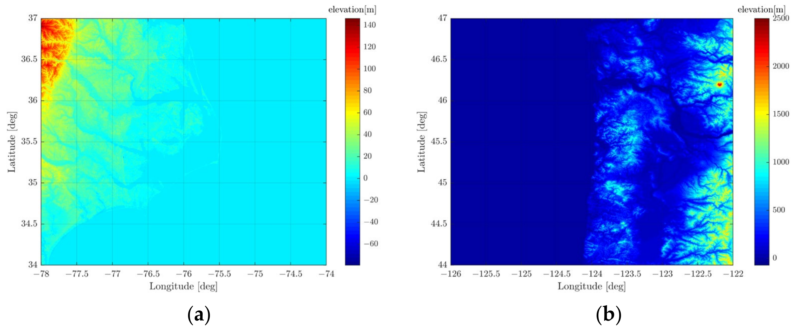
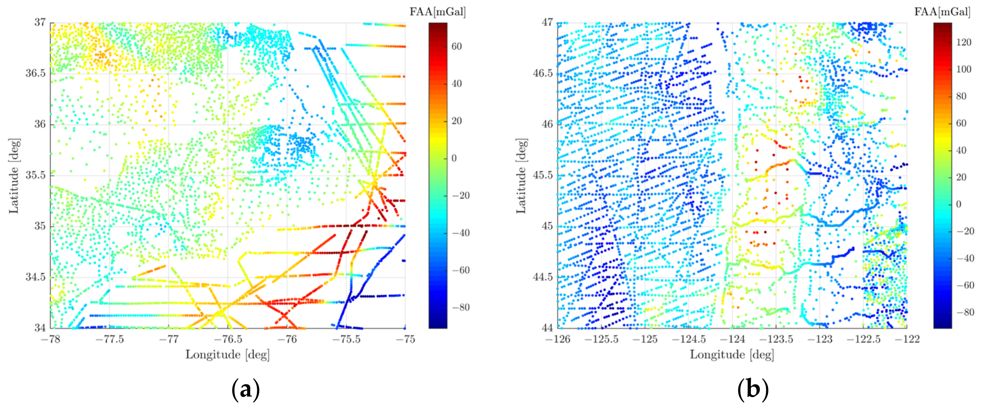
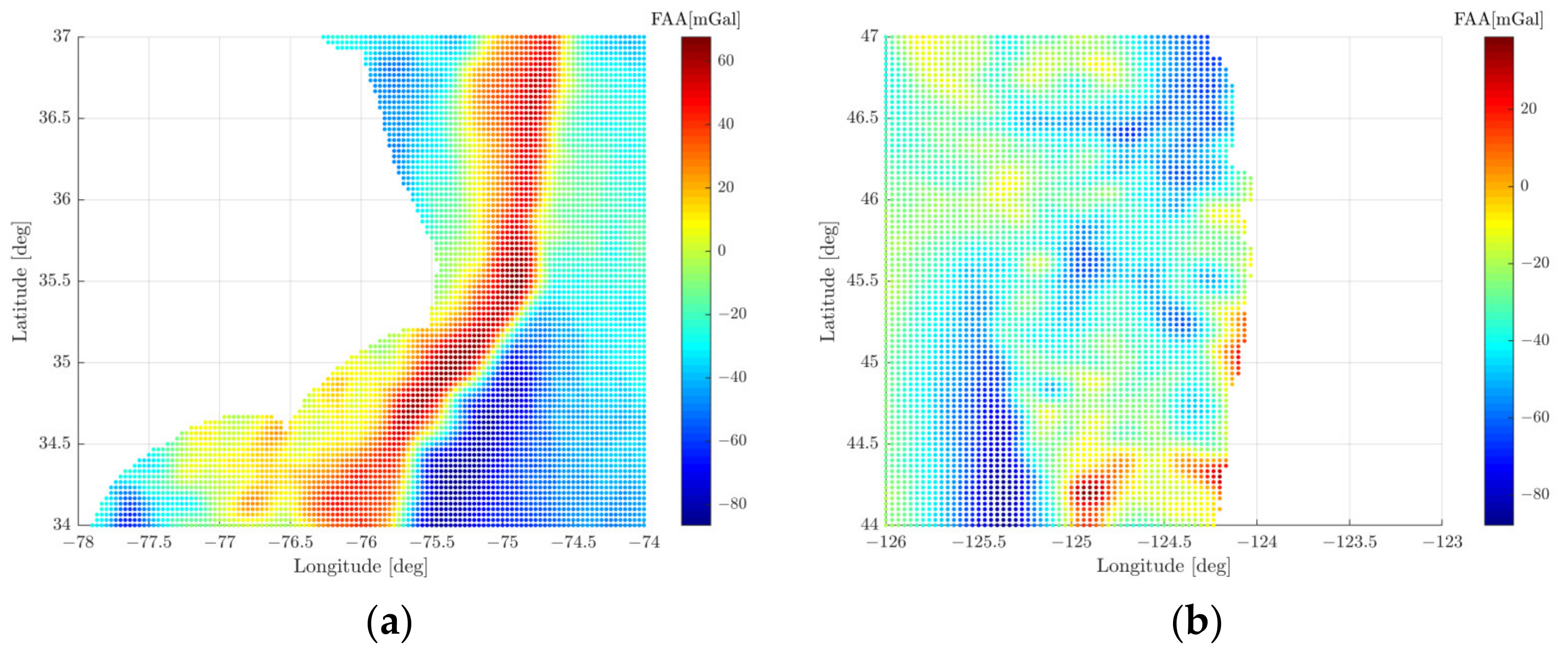
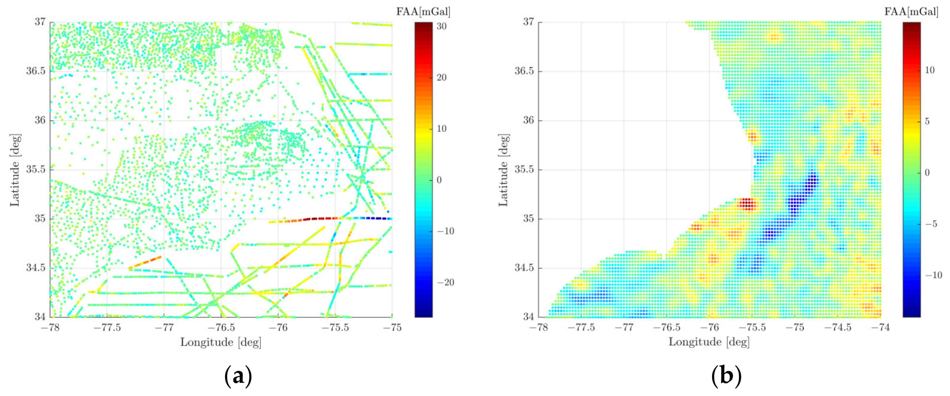
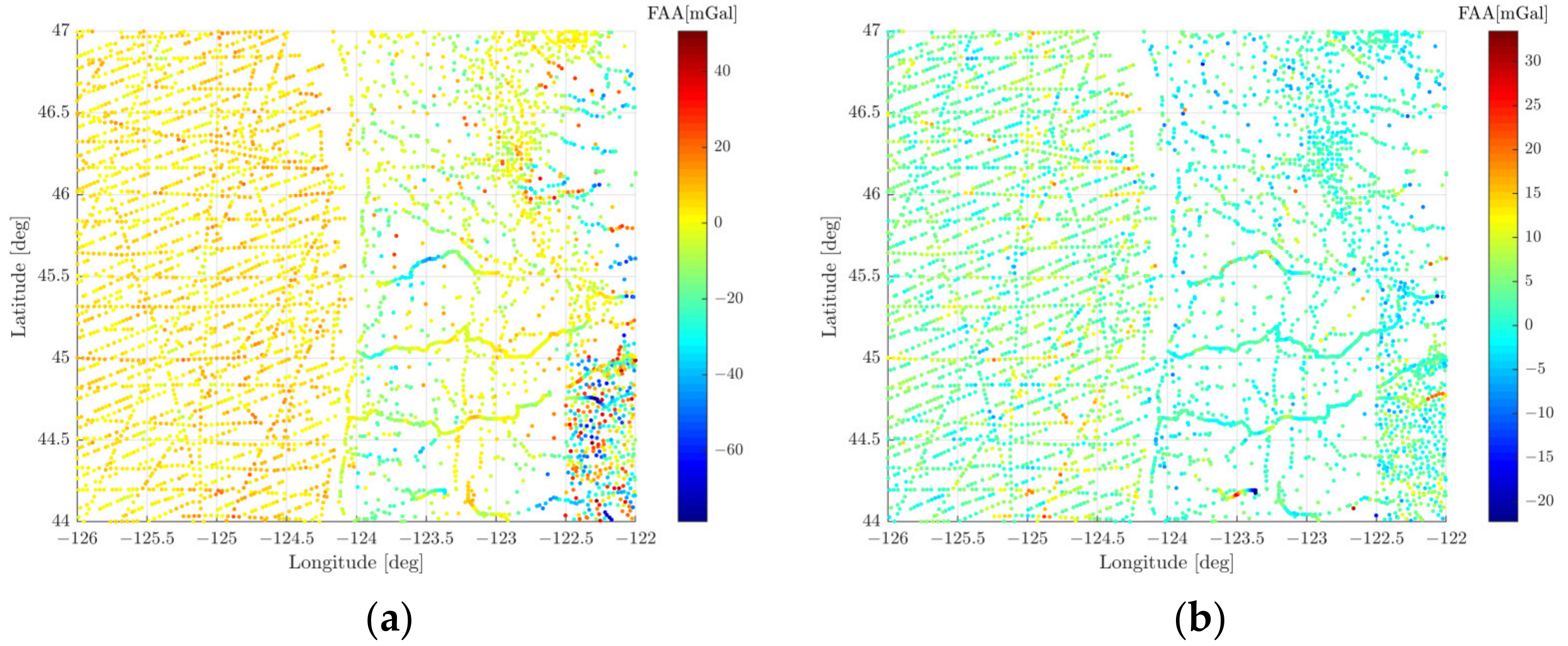
The gravity data used in the experiments include measured terrestrial, shipborne, airborne gravities and gravity anomalies derived from satellite altimetry. Terrestrial and shipborne gravity data come from the NGS99 gravity data set provided by the National Geodetic Survey (NGS). NGS99 is a compilation of the measured terrestrial and shipborne gravity data across the USA (data source: https://www.ngdc.noaa.gov/mgg/gravity/1999/data/regional/ngs99, accessed on 1 March 2021). The product provides free-air gravity anomalies (FAA), Bouguer anomalies, etc., after a series of preprocessing. In the east coast experiment area, we use 2860 terrestrial gravity points and 1678 shipborne gravity points, which are shown in Figure 2a. The distribution of shipborne gravity points is uneven, which is reflected in the dense distribution of data on the shipping route but many gaps outside the route. The shipborne gravity signals vary greatly, while the terrestrial gravity signals vary more gently and are densely distributed in most areas. In the west coast experiment area, there are 2814 terrestrial gravity points and 2288 shipborne gravity points, as shown in Figure 2b. Different from the east coast experiment area, the distribution of shipborne gravity points in the west coast area is more even.
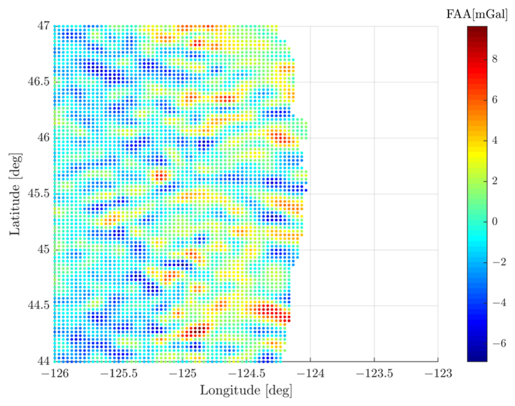
Due to the data gaps between ship lines, satellite altimetry and airborne gravities with more uniform distribution are needed as supplements. Satellite altimetry used in this article are DTU15 gravity anomalies with a 2′ resolution (data source: https://ftp.space.dtu.dk/pub/DTU15, accessed on 1 March 2021). Under the influence of the complex terrain on the ground, the accuracy of gravity anomalies inversed from satellite altimetry in inshore areas is not so good, but their high resolution and uniform distribution can make up for the deficiency of shipborne gravity to a certain extent. The distribution of DTU15 on sea is shown in Figure 3.
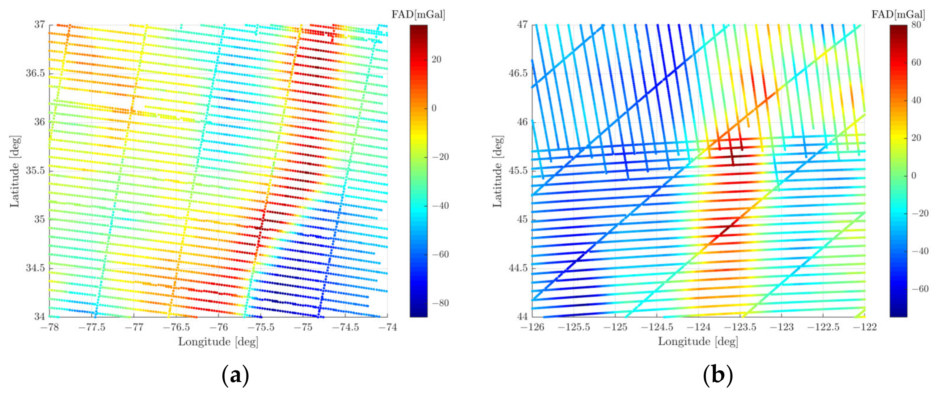
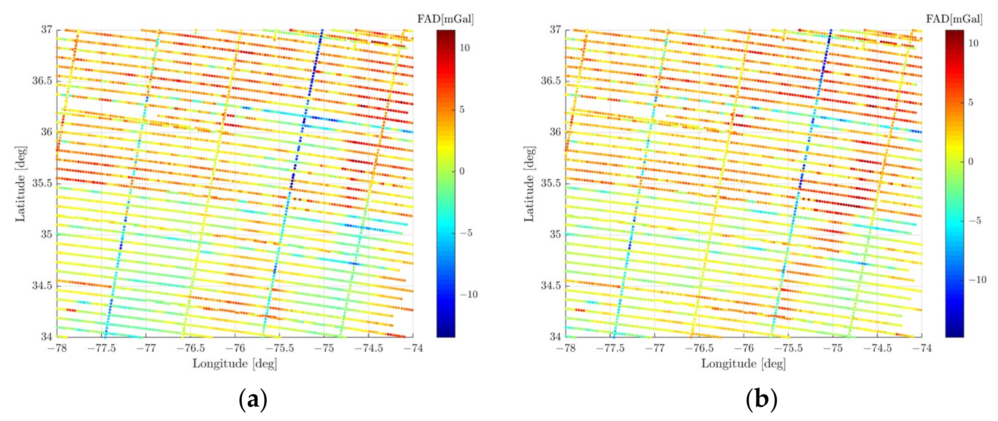
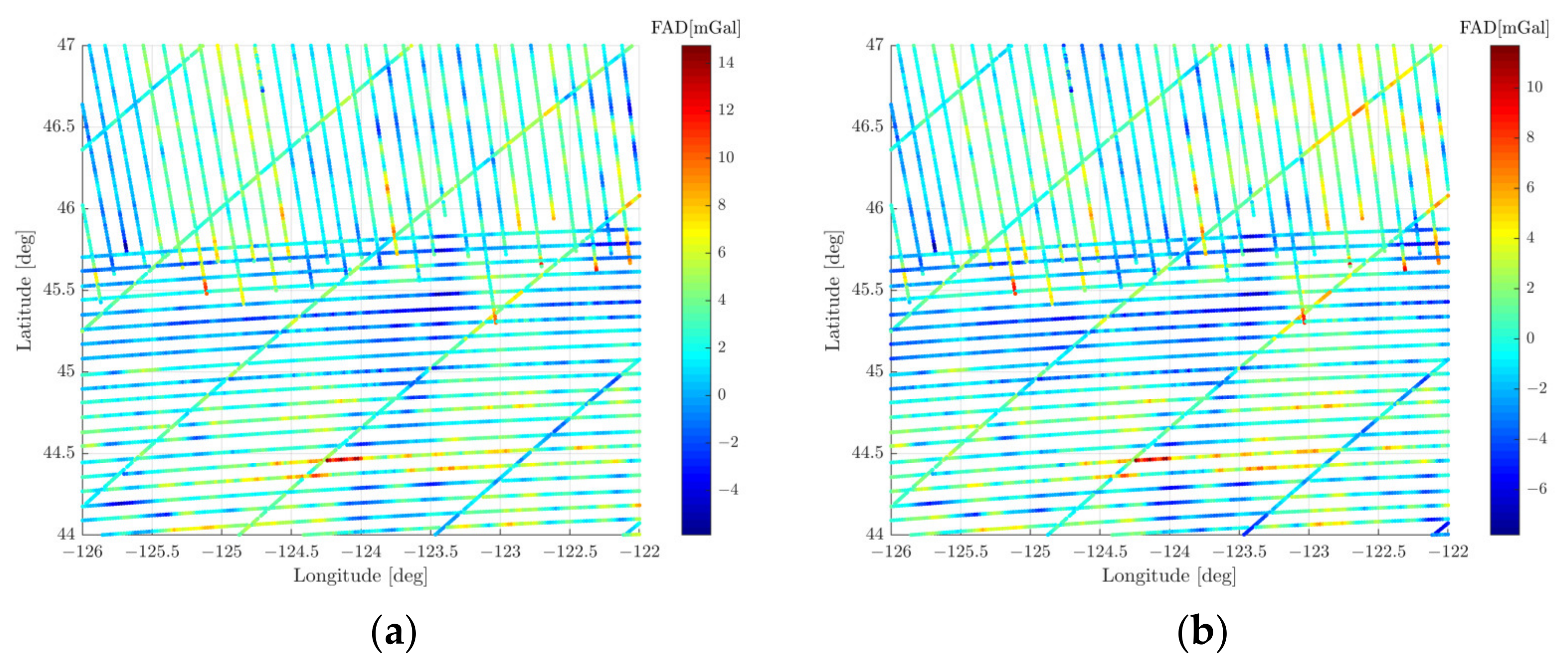
Airborne gravity data come from the GRAV-D project, which is developed by the NGS to redefine the vertical datum of the USA. GRAV-D currently covers most areas of the USA, providing full-field gravity data, which can be turned into free-air gravity disturbances (FAD) or free-air gravity anomalies (data source: https://www.ngs.noaa.gov/GRAV-D, accessed on 1 March 2021). In the east coast experiment area, 5367 airborne gravity points are selected, and their average flight altitude is approximately 5460 m. In the west coast experiment area, the number of airborne gravity points is 7458, and the average flight altitude is approximately 6938 m. The distribution of airborne gravity data is shown in Figure 4. Airborne gravity data have high resolution and uniform distribution, so they are not limited by ground terrain conditions. The shortcoming of airborne data is that the high flight altitude leads to low data accuracy, thus it is difficult to simulate the full-band gravity signal on ground points.
GPS/leveling data are used to verify the accuracy of the unified land–ocean quasi-geoid (data source: https://geodesy.noaa.gov/GPSonBM, accessed on 1 March 2021). In the east coast experiment area, due to the flat land terrain, there are many measured GPS/leveling points with a total of 807, which is 177 in the west coast experiment area, as shown in Figure 5. GPS and leveling surveys are impossible to be carried out offshore. So, this article uses GPS/leveling points along the coast to check the accuracy level of the unified land–ocean quasi-geoid on sea.
2.2. RBF Modeling Strategies
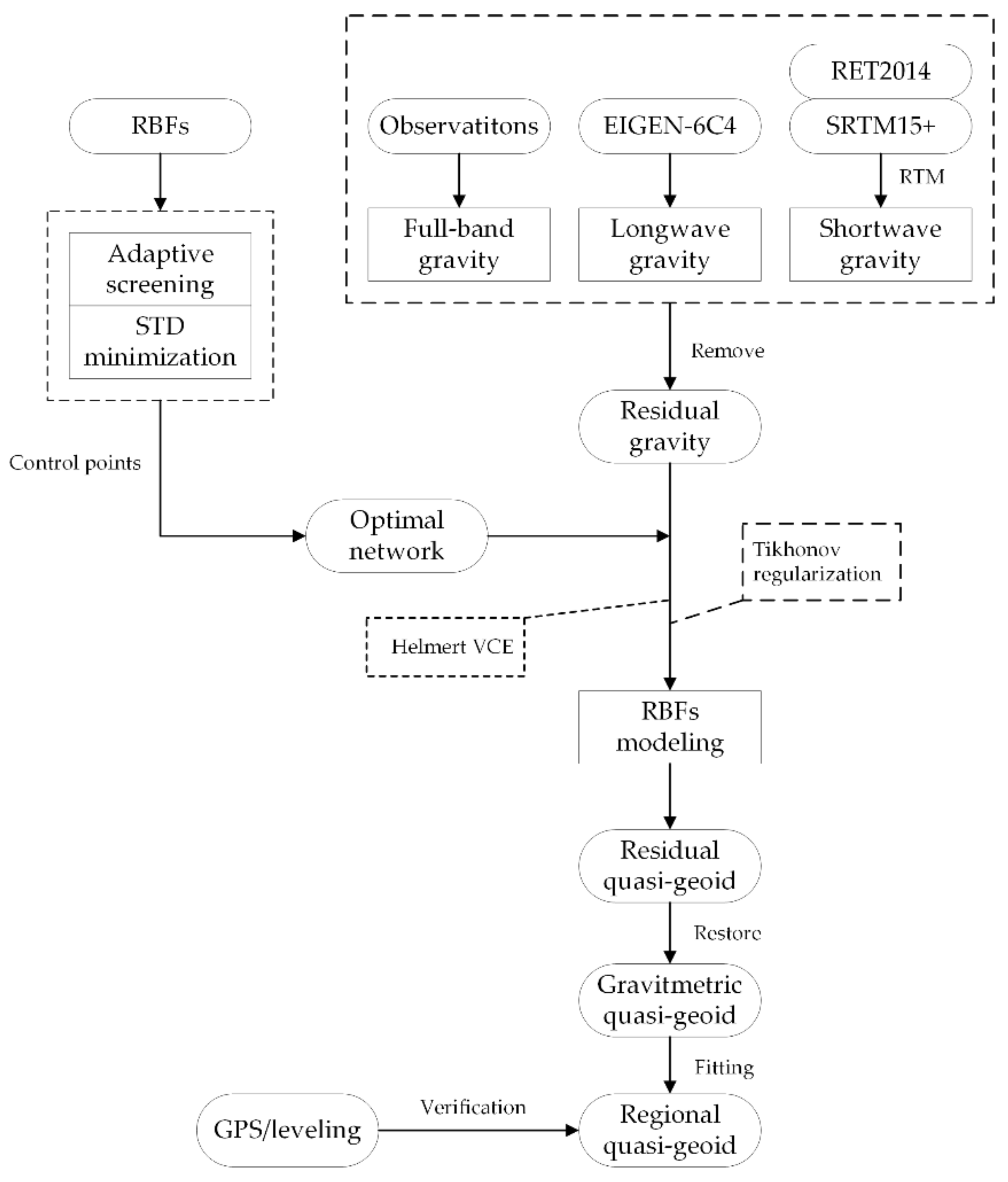
In this article, the local quasi-geoid is calculated based on the RBF model following the basic framework of the RCR technique [35]. After removing GGM and terrain effects from gravity observations, the residual gravity is included in the RBF model as input data. Helmert VCE is used to evaluate various observations [36]. Tikhonov regularization is used to solve ill-conditioned problems that may occur in the design matrix. A small number of points are selected from GPS/leveling data as control points, and the remaining data are as internal checkpoints. Under the constraint of control points, the optimal RBF network is determined to construct the model. The quasi-geoid calculated is compared with internal checkpoints, and the standard deviation (STD) of the difference between them is taken as the accuracy indicator. The flowchart is shown in Figure 6.
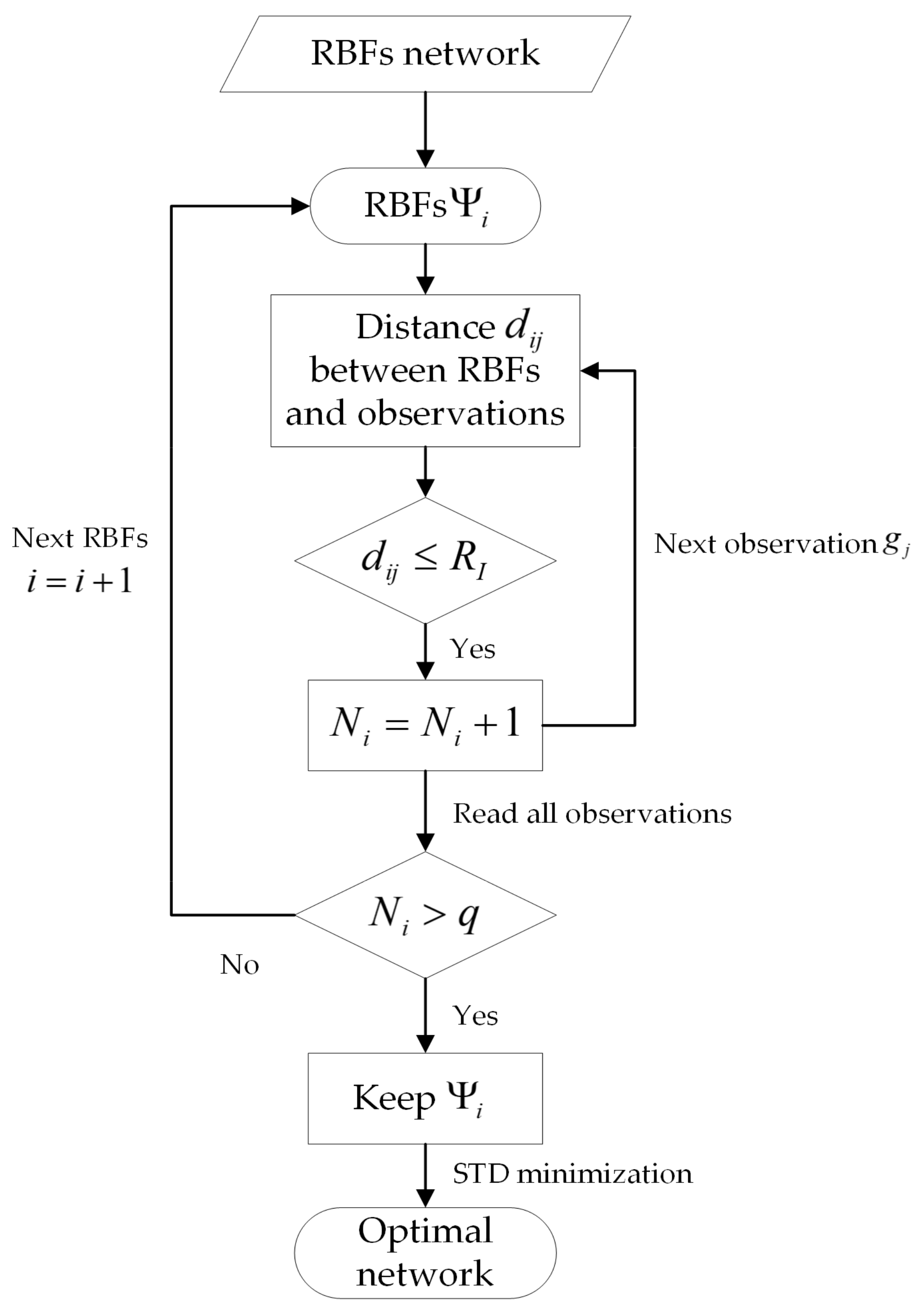
When the spherical grid is used to place the RBFs, not all grid points should be included in the model, which is because the RBFs have strong localization characteristics, and their energies are mainly concentrated around the center. So, the observations near RBFs are the main contribution to the simulated gravity signal. If the RBFs without enough observations around are included in the model, the local gravity field will be over-parameterized, and the reliability of the model solution will be reduced. In order to locate and eliminate the redundant RBFs, it is usually necessary to introduce a filter radius :
where is the number of RBFs; denotes the correlation length of RBFs, which specifically refers to the straight-line distance between the RBFs and observations when the absolute value of RBFs decays to half of the maximum value. represents correlation length parameter. With the center of RBFs as the spherical center, if the number of all observations within the radius is greater than , the RBFs will remain; otherwise, they will be excluded. and need to be determined based on the actual situation. In this article, we specify . ranges between 50 and 90 km. We determine the suitable value of through some trial calculations, ensuring meets the modeling requirements. The general adaptive screening process is shown in Figure 7.
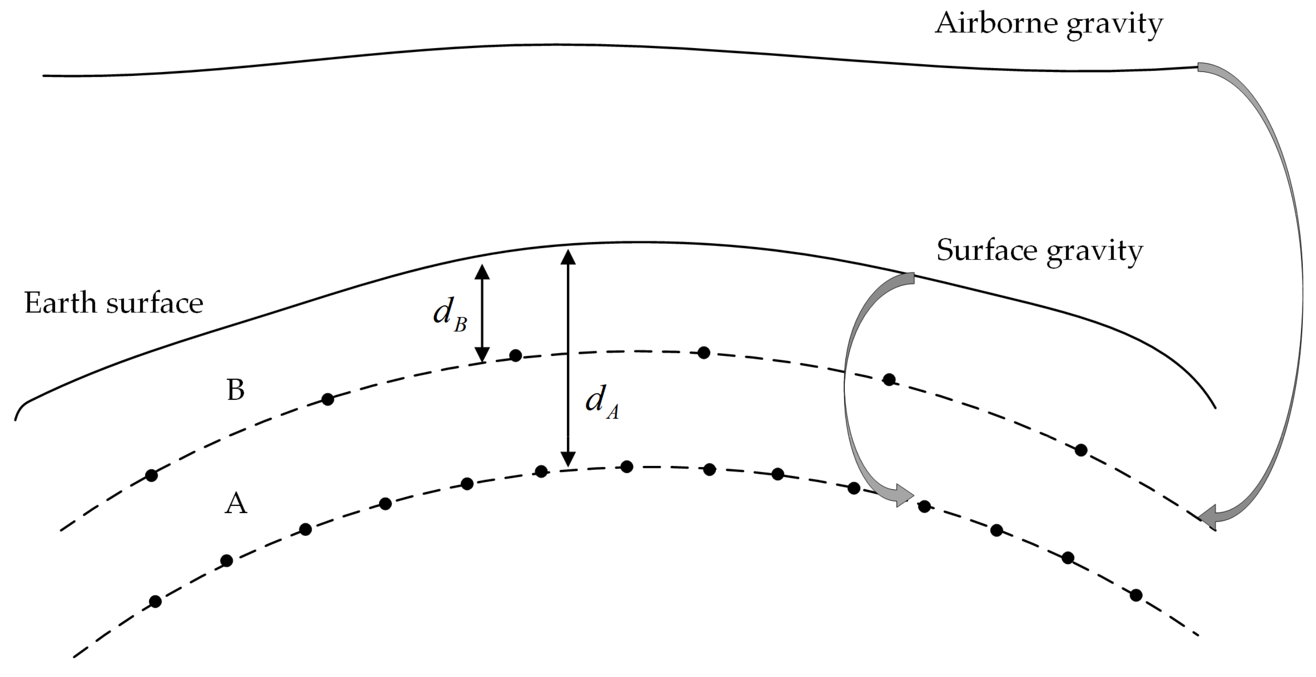
Considering the altitude of airborne gravity data is much higher than the terrestrial, shipborne and satellite altimetry data, the one-layer RBF network cannot simulate the full gravity signals well. Therefore, we design a multi-layer RBF network to fuse these four types of data, which are shown in Figure 8. We are currently only using two layers, and more layers are of course encouraged to be used.
In Figure 9, surface gravity denotes terrestrial, shipborne and satellite altimetry data; and denote the depth of grid A and B. The specific modeling process is as follows:
- GGM and RTM are removed from the terrestrial, shipborne and satellite altimetry observations to obtain residual gravity anomalies, . The RBF network A is determined by the STD minimization. After the three kinds of gravity data are fused to calculate the RBF model parameters, the airborne gravity points are taken as prediction points and the corresponding model gravity disturbance will be calculated.
- Remove GGM and from the airborne gravity to obtain residual gravity disturbances, . The RBF network B is determined by STD minimization and then the corresponding RBF model parameters will be calculated.
- Based on the RBF networks A and B, the height anomalies on unknown points are computed, respectively, and added together. Then GGM and RTM signals are restored then to obtain the final quasi-geoid.
2.3. RBF Modeling Methodology
RBF is a nonlinear function with the local characteristic and radial symmetry. In essence, the RBF model only depends on the relative position relationship between the computed points and the center of RBFs. Represent the spatial position of RBFs as , which is usually placed on a sphere inside the Earth such as the Bjerhammar sphere. The point outside the sphere is used to represent the spatial position of the observations. RBFs can be expressed as:
where denotes the radius of the Bjerhammar sphere; denotes the Legendre polynomial of degree m; is the Legendre coefficient, which is the shape factor of RBFs, determining their properties in the spatial and frequency domain; and are the unit vector of and . Define the depth of RBFs as: .
According to the Runge–Krarup principle, the external disturbing potential can be approximated by a harmonic function completely embedded inside the Earth. So, the linear combination of RBFs can be used to approximate :
where denotes the number of RBFs; denotes the unknown coefficient of the RBF model.
Based on the RCR technique, can be decomposed into three components:
where denotes long-wave signals represented by GGM; denotes high-frequency gravity information implied by terrain masses, used to represent short-wave signals; denotes residual disturbing potential. According to the functional relationship between the observations and , the linear combination of RBFs can be further used to simulate the observations:
where ; denotes residual gravity anomaly; denotes residual gravity disturbance; denotes residual height anomaly. In this article, all geoid undulations have been converted to height anomalies (GPS/leveling observations), ensuring the unity of elevation datum:
where denotes bouguer gravity anomaly; denotes mean normal gravity; denotes the topographic height. It is worth noting that the above formula is an approximate formula.
Equation (5) can be abstracted as a linear observation model:
where denotes the observation vector of class ; is the vector of model coefficients; is the error vector. The equation can be solved using the least-squares estimation. Due to the lack of the prior information related to the error of observations, the weight of all kinds of observations can be determined by the VCE technique.
2.3.1. Characteristics of RBFs in the Spatial Domain
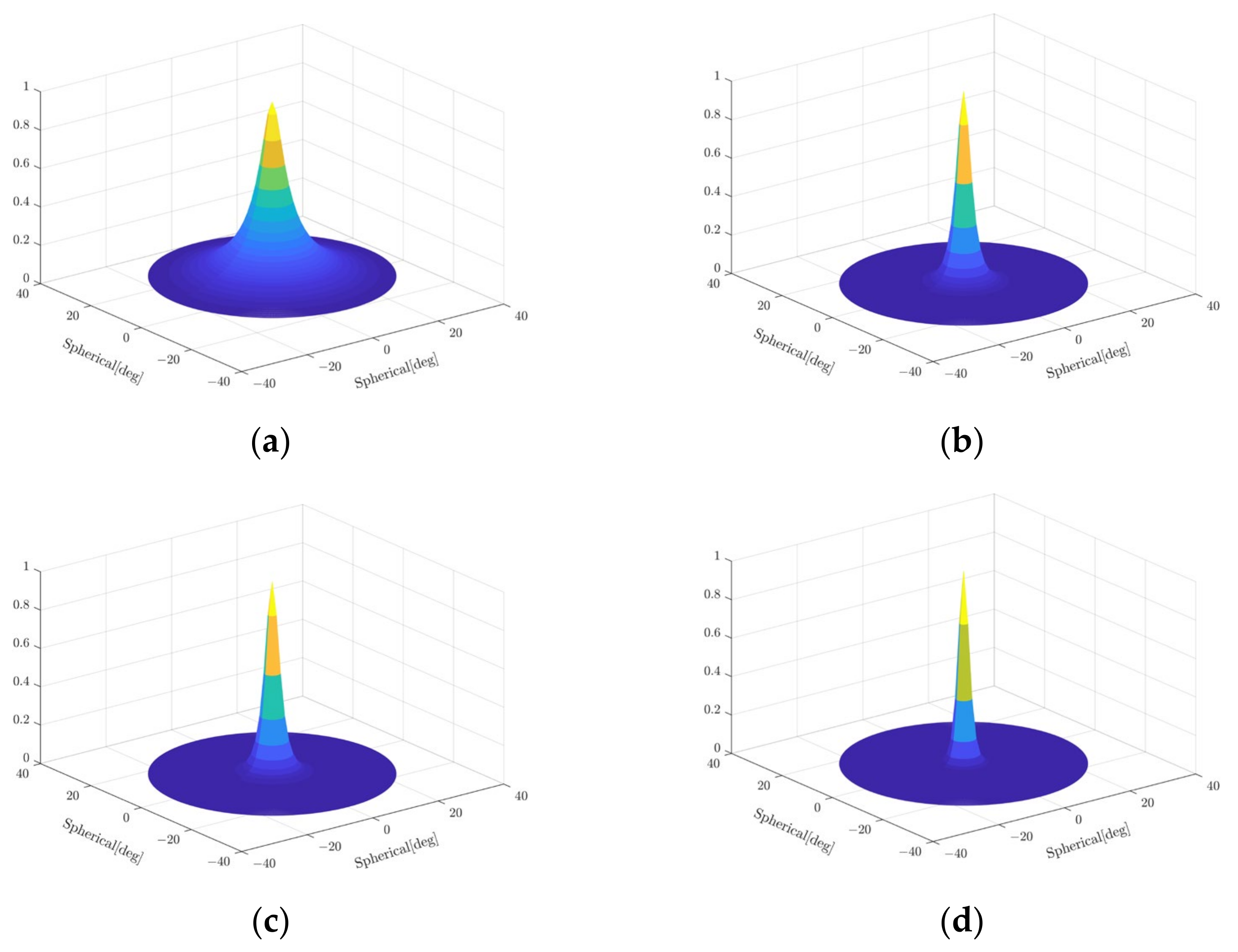
Several types of RBFs widely used in local gravity field modeling are as follows: the IMQ kernel, the Poisson kernel, the radial multipoles kernel and the Poisson wavelets kernel, represented by , , and respectively. We use these RBFs’ analytical expressions to construct the model. See the related research for their specific formulas [37]. Convert the analytical formula of RBFs to the unit sphere, and then, respectively, draw their pictures in the spatial domain when , as shown in Figure 9. It can be seen from the figure that RBFs have obvious localization characteristics. In the position far from the center of RBFs, the signals’ energies rapidly decay, which is conductive to the concentration of local gravity signals.
2.3.2. RBF Networks
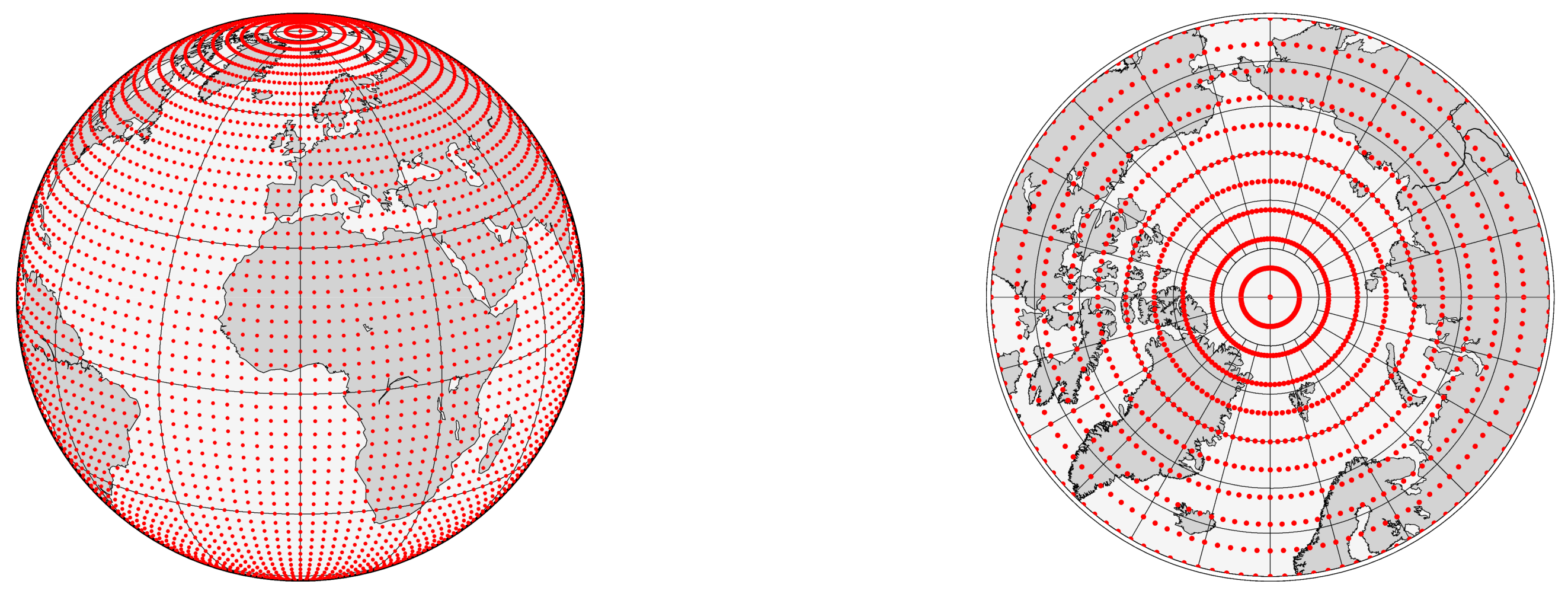
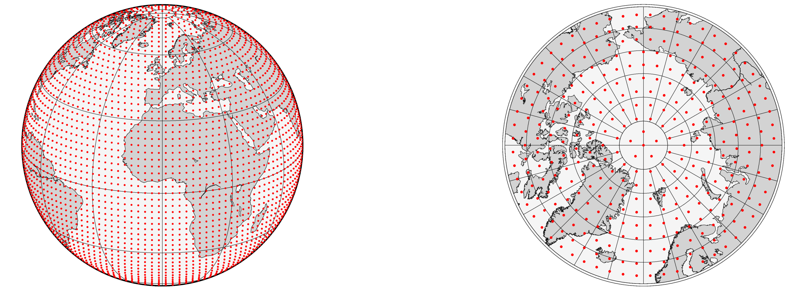
The design of the RBF network is divided into the determination of the sphere position and the buried depth. There are mainly two strategies to determine the sphere position of RBFs. One is to directly place RBFs under observations, which is extremely dependent on the spatial distribution of observations. The other is to place RBFs on the regular grid, which can make RBFs evenly distributed in the computation areas. At present, the second strategy is more commonly used, which is also adopted in this article. The simplest regular spherical grid is a geographical grid, which is one kind of isogonal grids. Geographical grid nodes space along the longitude circle and latitude circle with equal-angle intervals. Figure 10 shows its distribution globally and in the Arctic.
It can be clearly seen from Figure 11 that the geographical grid is very unevenly distributed in high-latitude regions. The higher the latitude is, the denser the grid dots are. In a slightly large area, such a defect will become more obvious. In view of this phenomenon, scholars propose a kind of spherical isometric grid, the Reuter grid, which ensures that the spherical distances between grid dots in meridian and latitude direction are equal, so that RBFs can be distributed evenly in high-latitude regions, as shown in Figure 11. The specific formulas can be found in the relevant articles [32].
The determination of the optimal RBF network is always the focus and difficulty in RBF modeling. When RBFs are buried deep, the gravity signals simulated by the model are mainly concentrated at low frequencies. This kind of model has strong stability but leads to the simulated gravity signals being coarse due to omission errors. The shallower the buried depth of RBFs is, the more sensitive they are to the high-frequency signals such as terrain masses. The stability of the model will be reduced, and ill-conditioned problems may occur. When the number of RBFs is too large caused by high grid resolution, the overlap between RBFs will increase, which leads to the RBFs model being over-parameterized. On the contrary, too few RBFs are insufficient to simulate full gravity signals.
When the RBF model is constructed using discrete gravity points, it is difficult to uniquely determine the appropriate position of RBFs by theories before modeling. Scholars generally use posterior statistical methods such as GCV, RMS or STD minimization technique to screen out the optimal RBF network [27]. In this article, the STD minimization technique is adopted to design the RBF network. This method is simple and efficient, but it lacks strict a theoretical basis. The STD minimization technique divides a certain range of grid resolutions and depths into different combinations according to a certain step. These combinations are, respectively, used for modeling and compared with the control points. The combination achieving the smallest standard deviation is determined as the optimal RBF network.
2.3.3. Tikhonov Regularization Technique
When directly using discrete data for modeling, the ill condition of the design matrix may occur due to the uneven distribution of observations and the excessive number of RBFs. Considering the lack of the sufficient prior information of observations, Tikhonov regularization is introduced to deal with the ill-conditioned problems [38]. Tikhonov regularization meets the following estimation criteria:
The general estimation formula is written as:
where is the regularization matrix; is the regularization parameter. In this article, is assumed to be the identity matrix, i.e., . After singular value decomposition (SVD), the regularization solution can be obtained as:
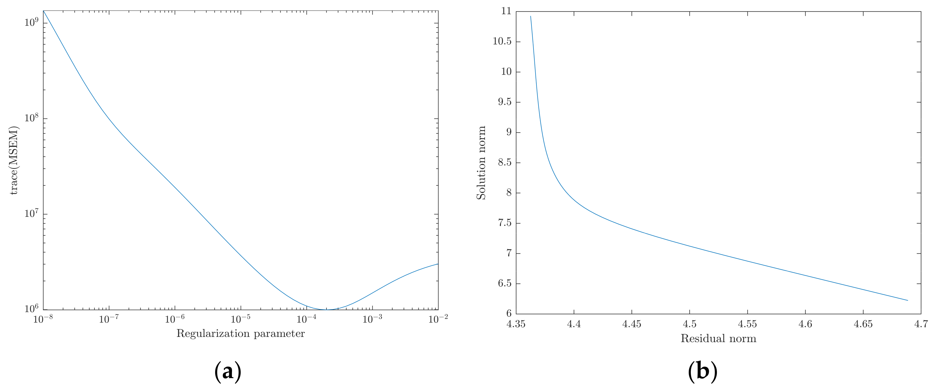
The regularization parameter is determined by the following two methods: the MSE and L-curve techniques. The basic principle of the MSE technique is as follows:
where . denotes the truth value of unknown parameter . We usually use the estimated result to replace , which will affect the optimality of regularization parameter to some extent.
The L-curve technique is used to find the best one from different regularization parameters to achieve the optimal balance between the residual sum of squares and the smoothness of regularization function . Construct a curve with as abscissa and as ordinate. The point with maximum curvature (inflection point) corresponds to the optimal regularization parameter.
2.3.4. Residual Terrain Model
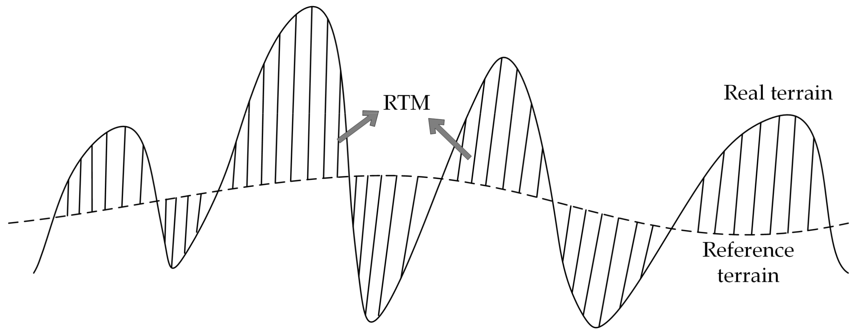
The high-frequency gravity signals implied by the terrain mass have an important influence on local gravity field modeling, especially in mountainous areas [39]. RTM can be used to represent terrain effects [40,41,42]. The RTM technique is essentially the differences between the real terrain and the reference terrain, as shown in Figure 12. The real terrain surface usually denotes digital terrain model (DEM) with a high resolution. The reference terrain is relatively smooth with a lower resolution, which can be computed from the spherical harmonic terrain model such as RET2014 [43]:
where ; denotes full normalized height coefficients. Based on Forsberg’s classic TC program, RTM results can be well calculated.
3. Results
This section describes in detail the experiment process and the results of calculating the unified land–ocean quasi-geoid from heterogeneous data sets based on RBFs. Compared with the results of the Stokes integral, the advantages of RBFs in multi-source data fusion are proved.
3.1. The East Coast Experiment Area of the USA
Based on the RCR technique, EIGEN-6C4 (degree 2190) gravity anomalies are removed from the measured terrestrial, shipborne and DTU15 data, as shown in Figure 13. Detailed statistics of the residual gravity anomalies are shown in Table 1, which shows that the residual terrestrial gravity signals are the smoothest. The amplitude of shipborne residual gravity anomalies is the largest, whose STD reaches 5.261 mGal. The terrain of the experiment area is quite flat, so the impact of terrain masses can be ignored, seen from the value of and in Table 1.
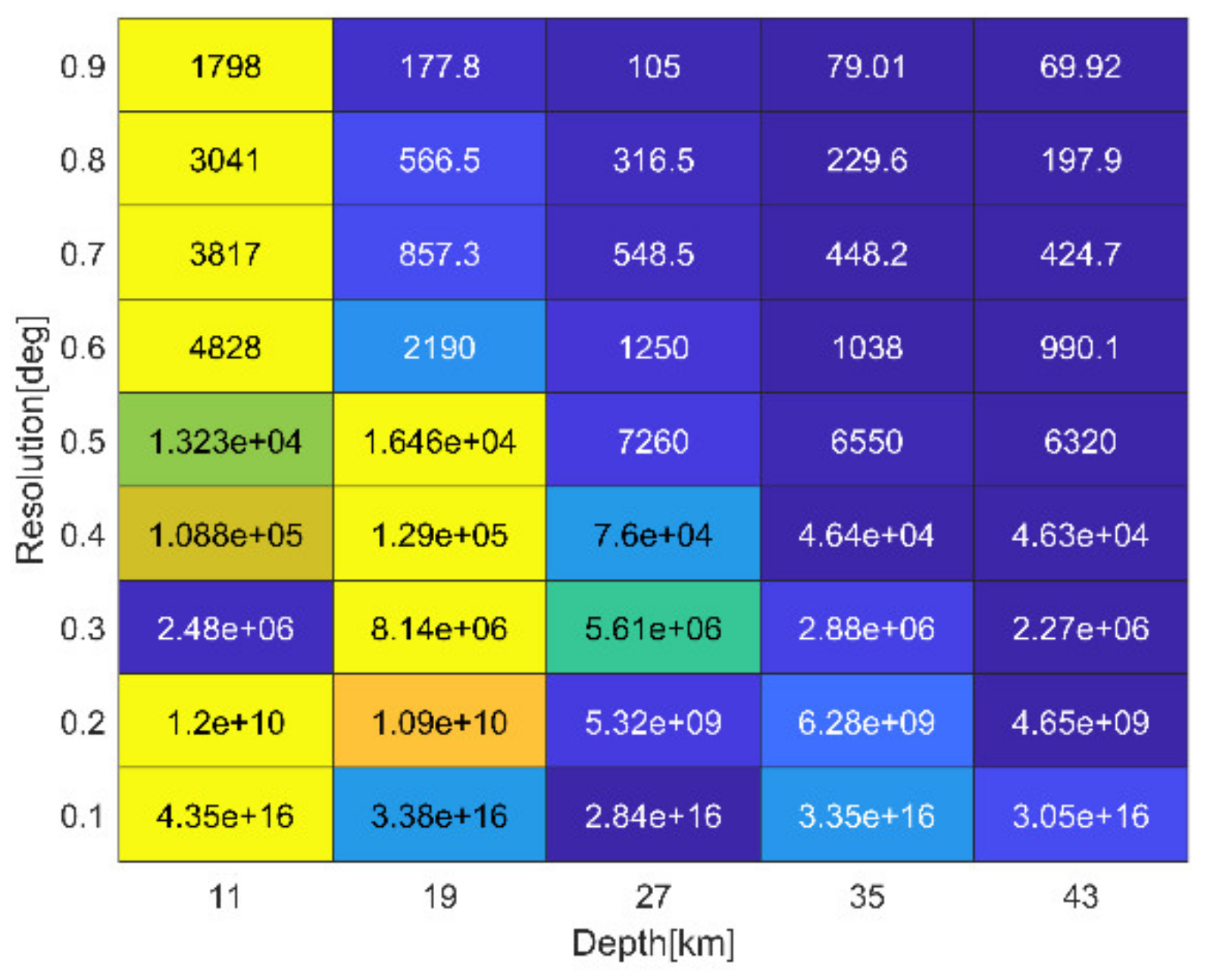
Firstly, we use terrestrial and DTU15 gravity anomalies for modeling, considering the shipborne data in this zone are few and unevenly distributed. Set the grid resolution range to 0.1°~0.9° and the step size be 0.1°; set the depth range to 10~50 km and the step size be 1 km. The (part of) condition number of the design matrix is counted as shown in Figure 14. It can be seen from the figure that the lower the grid resolutions and the deeper the depths are, the smaller the condition number is. Otherwise, the condition number will be larger, making the ill condition more serious.
Taking the combination with resolution of 0.1° and depth of 11 km as an example, the number of RBFs is 2324 and the condition number of the design matrix is . The accuracy of the ill-conditioned model is m checked by control points. Use the MSE method and the L-curve method, respectively, to determine the regularization parameter, as shown in Figure 15. The results show that the optimal regularization parameters determined by the MSE and L-curve methods are all , and the accuracy of the geoid calculated using this parameter is 6.9 cm, which is a great improvement compared with the original modeling result.
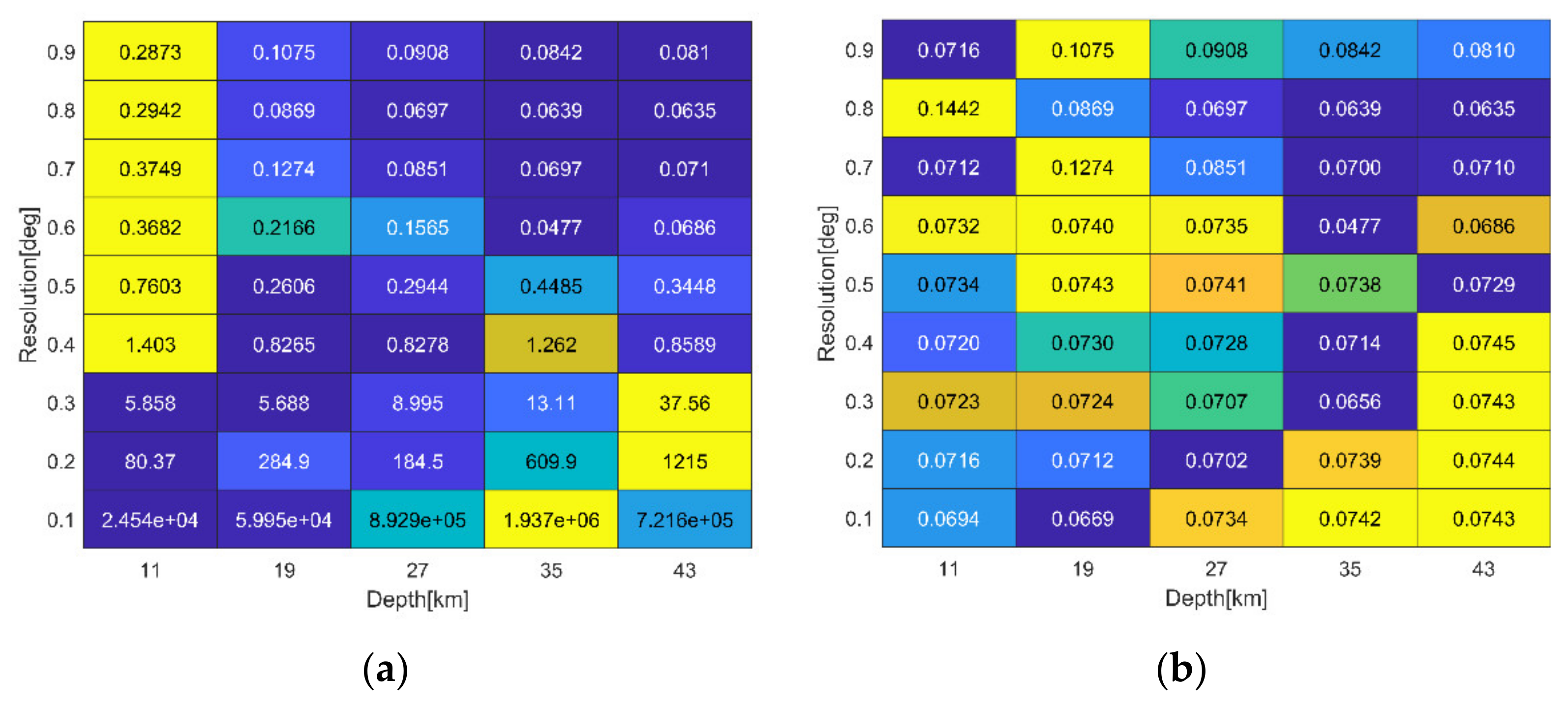
The calculation results of all combinations of resolutions and depths are shown in Figure 16. Figure 16a shows the accuracy of original modeling without regularization; the accuracy of RBF modeling using Tikhonov regularization is shown in Figure 16b. As can be seen in Figure 16, when the condition number is greater than 1000, the serious ill-conditioned problems lead to the gradual deviation of the modeling results from the normal values. In particular when the grid resolution is over 0.3°, the accuracy of the model geoid is lower than the meter level. Using the Tikhonov regularization technique, the accuracy of the ill-conditioned model is greatly improved to the centimeter level, which improves that Tikhonov regularization can effectively solve ill-conditioned problems in the RBF model.
Then shipborne gravities are added to terrestrial and DTU15 data sets. The weight ratio of terrestrial, DTU15 and shipborne data is 1:0.9410:0.0989 determined by the Helmert VCE technique. Fuse the three data sets to construct the RBF model with a grid resolution of 0.4° and a depth of 45 km, calculating regional gravity field at airborne points.
The distribution of airborne gravity disturbances after removing EIGEN-6C4 values is shown in Figure 17a. The fluctuation of airborne gravity signals is relatively stable. Gravity disturbances at airborne points are calculated based on the network A determined by terrestrial, DTU15 and shipborne data. Then are removed from the residual gravity in Figure 17a and as input data for the RBF modeling, as shown in Figure 17b. The statistical information of the two residual gravity disturbances is shown in Table 2.
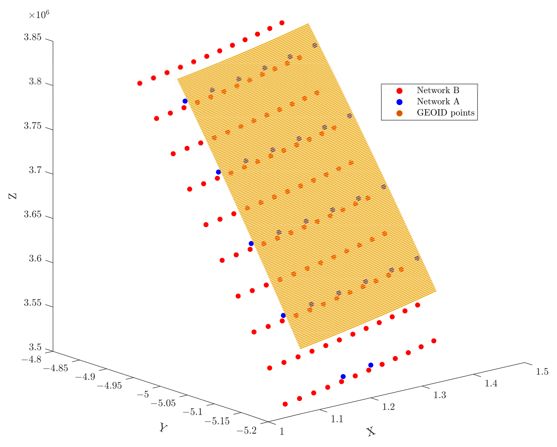
Based on the STD minimization technique, the network B is determined with a resolution of 0.8° and a depth of 16 km using as input data. The spatial distribution of networks A and B is shown in Figure 18, where the bottom blue dots refer to the network A; the red dots in the middle refer to the network B; the top yellow dots refer to the geoid grid points computed by the RBF model.
The RBF model is then constructed based on the network B, which is added together with the modeling result calculated by terrestrial, DTU15 and shipborne data based on the network A to obtain the final quasi-geoid, as shown in Figure 19a.
The quasi-geoid calculated by the RBF model is essentially a gravimetric geoid. It has a different datum than the GPS/leveling geoid, resulting in significant systematic errors. We use simple polynomial fitting to convert the datum of the gravimetric geoid to GPS/leveling geoid. The formula is as follows:
where denote fitting coefficients, i.e., bias parameter and tilt parameter; denotes the differences between the gravimetric geoid and the GPS/levelling geoid. denotes the center longitude and latitude. The order of the formula can be taken very high, but generally two orders is enough.
Considering the DTU15 data have already been introduced by the EIGEN-6C4 model, we also calculate the results without DTU15 gravity data, shown in Figure 19b. The calculation methods of the two geoids are the same.
The accuracy of the two quasi-geoids shown in Figure 19 is checked by the GPS/leveling data, respectively, on inland and coast, as shown in Table 3. On inland, the accuracy of the quasi-geoid fusing terrestrial, shipborne, DTU15 and airborne data is 1.9 cm, which is 1.3 cm on sea. After the DTU15 gravities are removed, the modeling accuracy is 1.9 cm inland and 1.2 cm on coast, not much different from the previous result.
3.2. The West Coast Experiment Area of the USA
The west coast of the USA has quite different topographic features from the east coast. Affected by the overall terrain high in the west and low in the east, the mountains in the west extend to the coastal zone, making the land–ocean boundary areas rugged, which brings many difficulties to the geoid calculation. Based on the RCR technique, EIGEN-6C4 gravity anomalies are removed from the measured terrestrial and shipborne gravity, as shown in Figure 20a. It can be seen from the figure that after the EIGEN-6C4 value is removed, shipborne gravity signals become relatively flat. There are serious omission errors in EIGEN-6C4 on terrestrial gravity points affected by the topographic relief. This article calculates RTM based on the prism integral to simulate high-frequency gravity signals and compensate for the omission errors existing in GGM.
In the calculation of RTM, the DEMs are usually expanded by approximately 2° from the edge of the gravity data area to avoid edge effects, as shown in Figure 21. The calculation efficiency can be improved by setting inner and outer computing regions. For example, the inner region within a 100 km radius uses high-resolution DEMs and the outer region within a 200 km radius uses low-resolution DEMs. The impact of terrain mass outside the outer region can be ignored due to the oscillating nature of RTM elevations [42].
The residual gravity anomalies obtained by removing RTM from the terrestrial observations are shown in Figure 20b, and their STD is reduced from 15.983 mGal to 4.134 mGal, indicating that the compensation for EIGEN-6C4 omission errors by RTM reaches approximately 74%. The residual DTU15 gravity anomalies are shown in Figure 22. The statistical information of various residual gravity data is shown in Table 4, which indicates that the variation range of residual DTU15 gravity anomalies is the smallest. The variation amplitude of residual terrestrial gravity anomalies is close to shipborne data.
Firstly, terrestrial and shipborne gravity data are used for modeling. The weight ratio of the two observations is 1:1.004 computed by the Helmert VCE technique, which shows that their accuracy level is close. Based on the STD minimization technique, the optimal RBF grid resolution is determined as 0.6° and the optimal depth is 22 km. Then we add residual DTU15 gravity anomalies to the terrestrial and shipborne gravity to construct the RBF model with an optimal grid resolution of 0.8° and an optimal depth of 26 km.
The distribution of airborne gravity disturbances after removing the EIGEN-6C4 value is shown in Figure 23a. The variation amplitude of residual airborne gravities is relatively small. Based on the RBF network A determined by terrestrial, shipborne and DTU15 data, the model gravity disturbances are calculated on airborne points. Then are removed from the residual gravities in Figure 23a and as input data for the RBF modeling, as shown in Figure 23b. The statistical information of the two kinds of residual gravity disturbances is shown in Table 5.
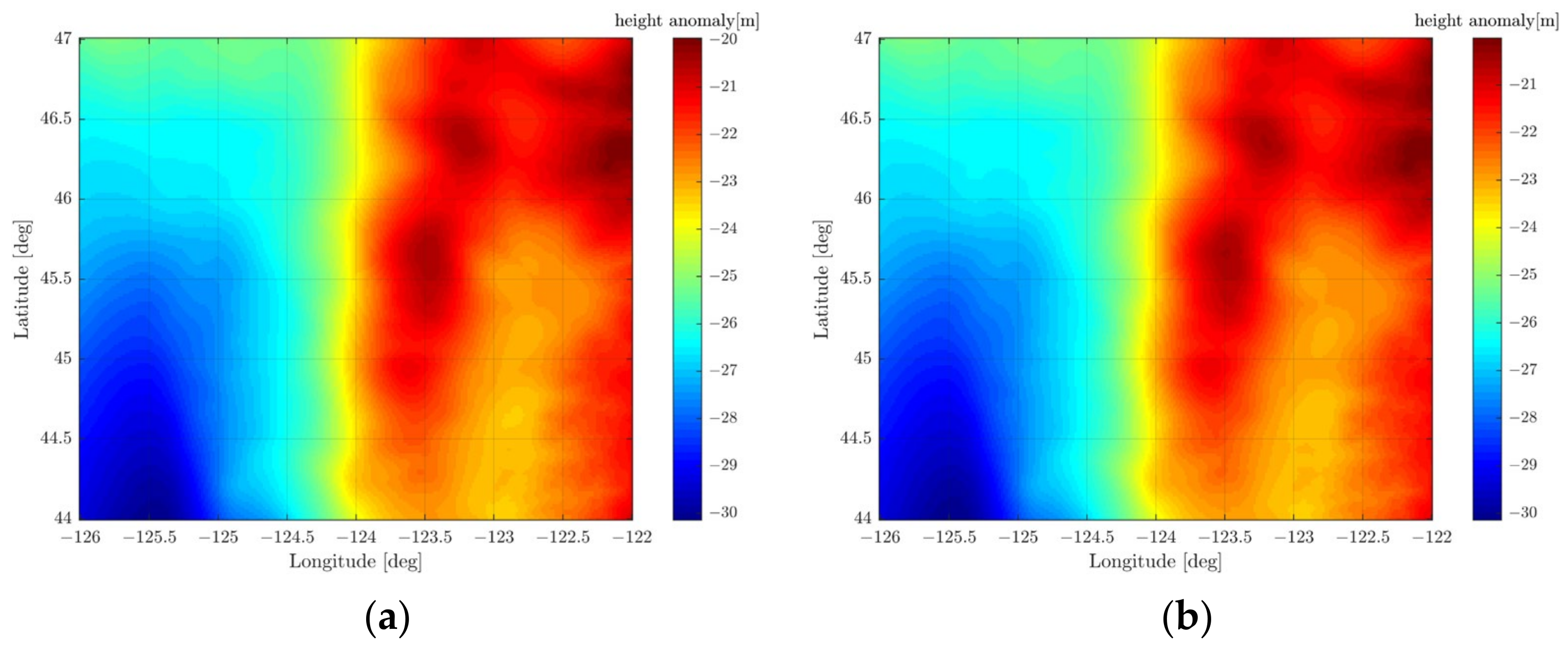
Based on the STD minimization technique, network B is determined with a resolution of 0.8° and a depth of 16 km. The RBF model is then constructed based on the network B, which is added with the modeling result based on the network A to obtain the final quasi-geoid, as shown in Figure 24a. We also calculate the results without DTU15 gravity data, shown in Figure 24b.
Check the accuracy of the three quasi-geoids shown in Figure 24 by 64 GPS/leveling points inland and 36 GPS/leveling points on coast, as shown in Table 6. The accuracy of the RBF model quasi-geoid is 2.2 cm inland, which is 2.1 cm on coast. After the DTU15 data are removed, the modeling accuracy is 2.0 cm inland and 2.1 cm on coast.
According to the results of the two experiments on the east and west coast, we consider that the accuracy of the unified land–ocean quasi-geoid can be improved by fusing heterogeneous data sets. Fusing terrestrial, shipborne, DTU15 and airborne gravities based on a multi-layer RBF network achieves great modeling accuracy both inland and on coast.
4. Discussion
Due to the complex topography of land–ocean junction areas, terrestrial and shipborne gravity measurements cannot be fully carried out. As it is also affected by the terrain, the accuracy of satellite altimetry data inshore is reduced. The airborne gravity is not limited by the terrain, but its accuracy will be lost with downward continuation. Therefore, the important premise of constructing a high-precision unified land–ocean quasi-geoid is to effectively fuse heterogeneous data sets. Considering the shortcomings of the commonly used integral algorithm, we use the RBFs to calculate the unified land–ocean quasi-geoid, the accuracy of which is improved by fusing more types of data sets. However, there are still some problems to be discussed and further studied, as follows:
- (1)
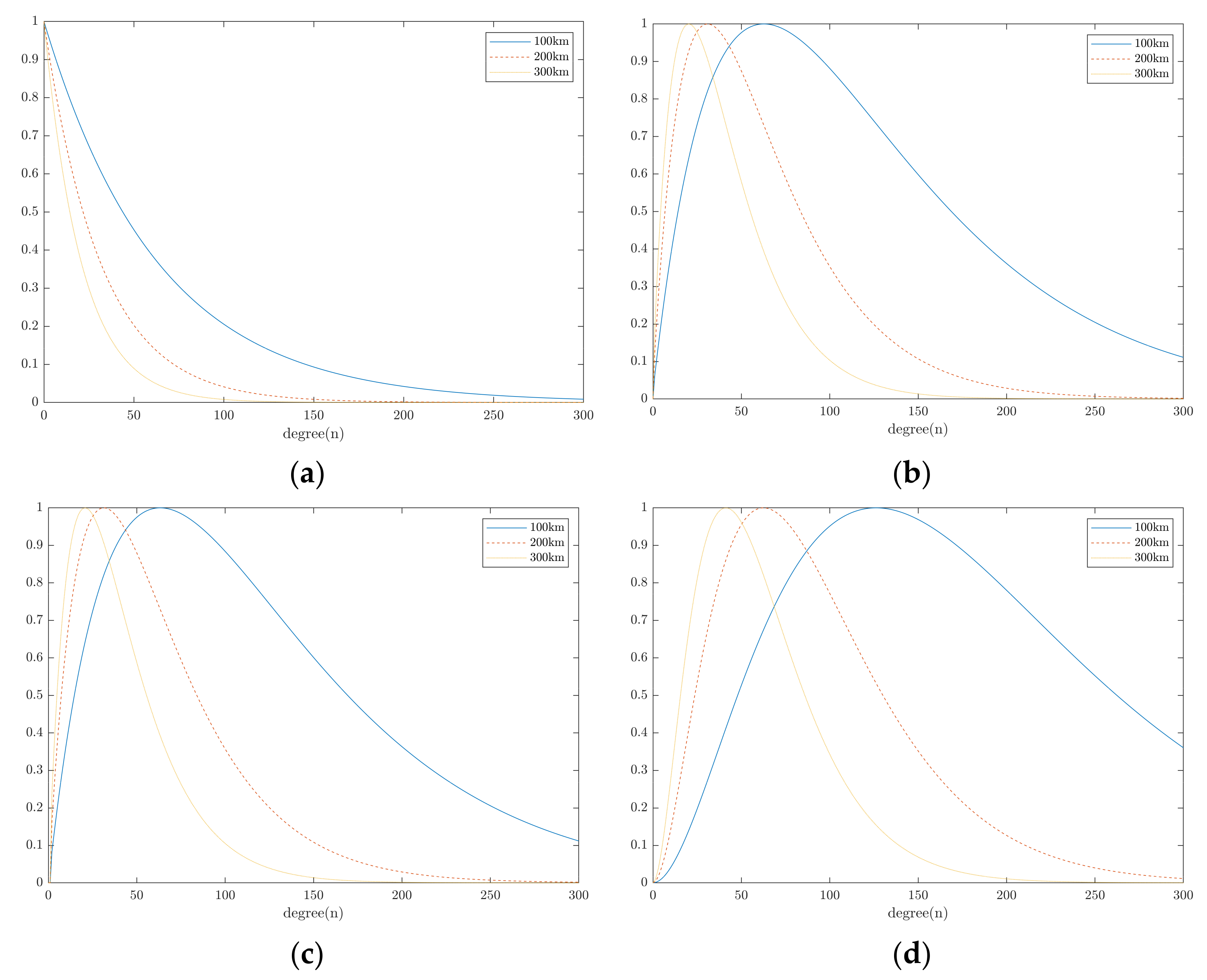
- The RBF used to calculate the land–ocean quasi-geoid in this article is the IMQ kernel, which has simpler function forms than the Poisson kernel, the radial multipoles kernel and the Poisson wavelets kernel. It can be seen from Figure 9 that the first-order Poisson wavelets kernel has the strongest localization characteristics when the depth is 300 km. However, the buried depth of RBFs will not be so deep generally when dealing with the measured data. When the buried depth is less than 100 km, the localization characteristics of various RBFs are all strong and their differences are quite small. By further analyzing the spectrum characteristics of RBFs, as shown in Figure 25, it can be seen that the Poisson kernel, the radial multipoles kernel and the Poisson wavelets kernel all have band-pass characteristics, while the IMQ kernel presents the characteristics of low-pass filtering. We have carried out some experiments to compare the modeling accuracy of the four RBFs. We preliminarily find that the low-pass characteristics of the IMQ kernel can help it filter out more high-frequency noise when dealing with the terrestrial gravity, making its modeling results slightly better than the other RBFs. The specific experimental results will not be presented in this article. Theoretically, the band-pass characteristics can help the RBFs simulate gravity signals more accurately. In this paper, the IMQ kernel is used to calculate the quasi-geoid for the time being, and the modeling differences between various RBFs will be more comprehensively analyzed in the future.
- (2)
- The STD minimization technique used to determine the optimal RBF network lacks a strictly theoretical basis, which is a compromise method in view of the lack of other more effective strategies. The reason why it is difficult to determine the RBF networks is that it is difficult to directly determine the appropriate positions of RBFs based on the prior information of discrete observations. If the gravity signals are gridded before modeling, we may directly determine the spatial position of the RBF points according to the resolution and height of the gravity grid. However, our goal is to model using discrete observations. The STD minimization technique can obtain good modeling results by screening lots of RBF networks, but it increases too much redundant calculations, which hinders the solution efficiency of the RBF model to a great extent. So, it is very important to develop a rigorous and logical method to determine the RBF networks.
- (3)
- The accuracy of the quasi-geoid fusing terrestrial, shipborne and DTU15 data is quite high, but the improvement is not obvious after adding airborne gravity. The main reason is that the gravity signals on airborne points simulated by network A is insufficient, resulting in little change in residual gravity disturbances after removing , as shown in Table 2 and Table 5. Theoretically, if the result of is significantly reduced, the function of the network B will be more obvious. In the future, we can further improve the multi-layer RBF network and try to set more layers of RBF grids, simulating the gravity signals more accurately.
5. Conclusions
This article designs a multi-layer RBF model to construct the unified land–ocean quasi-geoid fusing the measured terrestrial, shipborne, satellite altimetry and airborne gravity data in coastal areas. Several core problems in the process of RBF modeling are studied in depth. The local quasi-geoid with a 1′ resolution is calculated, respectively, on the flat east coast and the rugged west coast of the United States. Several conclusions are summarized as follows:
- (1)
- The behavior of four types of RBFs—the IMQ kernel, the Poisson kernel, radial multipoles and Poisson wavelets—is analyzed in the spatial domain. The figures show that RBFs have significant localization characteristics in the spatial domain, which is helpful to concentrate more gravity signals in local gravity field approximation. Placing RBFs on the geographic or the Reuter grid, the optimal RBF network, i.e., the optimal grid resolution and depth can be effectively determined based on the STD minimization technique.
- (2)
- The ill condition of the design matrix may occur due to the uneven distribution of observations and the excessive number of RBFs. Using the Tikhonov regularization technique, the accuracy of the ill-conditioned model is greatly improved to the centimeter level. The regularization parameters determined by the MSE and L-curve methods are basically the same. RTM calculated based on the prism integral algorithm can effectively simulate the high-frequency gravity signals implied by terrain masses and compensate for the omission errors existing in EIGEN-6C4. In the west coast experiment area, the compensation effect can reach approximately 74%. Therefore, in areas with large topographic relief, it is necessary to consider the influence of terrain masses on geoid calculations.
- (3)
- The local gravity quasi-geoids with a 1′ resolution are calculated by setting up multi-layer RBF networks based on the IMQ kernel, respectively, on the east and west coast of the United States. The results show that the accuracy of the quasi-geoid computed by fusing the terrestrial, shipborne, satellite altimetry and airborne gravity data in the east coast experimental area is 1.9 cm inland and 1.3 cm on coast after internal verification. The accuracy of the quasi-geoid calculated in the west coast experimental area is 2.2 cm inland and 2.1 cm on coast.
Through the above research results, we can roughly summarize the advantages of RBFs compared with other geoid calculation methods: (a) RBFs are simple and easy for multi-source data fusion; (b) RBFs can directly deal with discrete observations without gridding or downward continuation; (c) RBFs have a strong adaptive ability. In general, the RBF model has an important application value to calculate the unified land–ocean quasi-geoid from heterogeneous data sets.
Author Contributions
Conceptualization, Y.L. and L.L.; methodology, Y.L.; funding acquisition and project administration, L.L.; investigation and software, Y.L.; supervision and validation, L.L.; writing—original draft, Y.L.; writing—review and editing, L.L. All authors have read and agreed to the published version of the manuscript.
Funding
This research was funded by the National Natural Science Foundation of China, grant number 41874004.
Data Availability Statement
All data for this paper are properly cited and referred to in the reference list.
Acknowledgments
The authors are very grateful to the NGS, the DTU, the NOAA and the ICGEM for providing gravity, GPS/leveling, geoid and GGM data. The authors express thanks to Hirt and Tozer for providing DEM data. The software Gravsoft shared by Forsberg also helped a lot.
Conflicts of Interest
The authors declare no conflict of interest.
References
- Forsberg, R. Modelling the Fine-Structure of the Geoid: Methods, Data Requirements and Some Results. Surv. Geophys. 1993, 14, 403–418. [Google Scholar] [CrossRef]
- Alberts, B.; Klees, R. A Comparison of Methods for the Inversion of Airborne Gravity Data. J. Geodesy 2004, 78, 55–56. [Google Scholar] [CrossRef]
- Sabri, L.M.; Sudarsono, B.; Pahlevi, A. Geoid of South East Sulawesi from Airborne Gravity Using Hotine Approach. IOP Conf. Ser. Earth Environ. Sci. 2021, 731, 012014. [Google Scholar] [CrossRef]
- Strykowski, G.; Forsberg, R. Operational Merging of Satellite, Airborne and Surface Gravity Data by Draping Techniques. In Geodesy on the Move; Forsberg, R., Feissel, M., Dietrich, R., Eds.; International Association of Geodesy Symposia; Springer: Berlin/Heidelberg, Germany, 1998; Volume 119, pp. 243–248. [Google Scholar] [CrossRef]
- Knudsen, P.; Andersen, O.B. Improved Recovery of the Global Marine Gravity Field from the GEOSAT and the ERS-1 Geodetic Mission Altimetry. In Gravity, Geoid and Marine Geodesy; Segawa, J., Fujimoto, H., Okubo, S., Eds.; International Association of Geodesy Symposia; Springer: Berlin/Heidelberg, Germany, 1997; Volume 117, pp. 429–436. [Google Scholar] [CrossRef]
- Eppelbaum, L.; Katz, Y. A New Regard on the Tectonic Map of the Arabian–African Region Inferred from the Satellite Gravity Analysis. Acta Geophys. 2017, 65, 607–626. [Google Scholar] [CrossRef]
- Braitenberg, C.; Ebbing, J. New Insights into the Basement Structure of the West Siberian Basin from Forward and Inverse Modeling of GRACE Satellite Gravity Data. J. Geophys. Res. Earth Surf. 2009, 114, 1–15. [Google Scholar] [CrossRef] [Green Version]
- Neyman, Y.M.; Li, J. Modification of Stokes and Vening-Meinesz Formulas for the Inner Zone of Arbitrary Shape by Minimization of Upper Bound Truncation Errors. J. Geod. 1996, 70, 410–418. [Google Scholar] [CrossRef]
- Abbak, R.A.; Sjöberg, L.E.; Ellmann, A.; Ustun, A. A Precise Gravimetric Geoid Model in a Mountainous Area with Scarce Gravity Data: A Case Study in Central Turkey. Stud. Geophys. Geod. 2012, 56, 909–927. [Google Scholar] [CrossRef]
- Featherstone, W.E. Deterministic, Stochastic, Hybrid and Band-Limited Modifications of Hotine’s Integral. J. Geodesy 2013, 87, 487–500. [Google Scholar] [CrossRef] [Green Version]
- Wichiengaroen, C. A Comparison of Gravimetric Undulations Computed by the Modified Molodensky Truncation Method and the Method of Least Squares Spectral Combination by Optimal Integral Kernels. J. Geodesique 1984, 58, 494–509. [Google Scholar] [CrossRef]
- Nahavandchi, H.; Sjöberg, L.E. Precise Geoid Determination over Sweden Using the Stokes-Helmert Method and Improved Topographic Corrections. J. Geodesy 2001, 75, 74–88. [Google Scholar] [CrossRef]
- Tscherning, C.C.; Rapp, R.H. Closed Covariance Expressions for Gravity Anomalies, Geoid Undulations, and Deflections of the Vertical Implied by Anomaly Degree Variance Models; Scientific Interim Report Ohio State University: Columbus, GA, USA, 1974. [Google Scholar]
- Rapp, R.H. Gravity Anomalies and Sea Surface Heights Derived from a Combined GEOS3/Seasat Altimeter Data Set. J. Geophys. Res. 1986, 91, 4867. [Google Scholar] [CrossRef]
- Hwang, C. Analysis of Some Systematic Errors Affecting Altimeter-Derived Sea Surface Gradient with Application to Geoid Determination over Taiwan. J. Geod. 1997, 71, 113–130. [Google Scholar] [CrossRef]
- Hwang, C.; Guo, J.; Deng, X.; Hsu, H.-Y.; Liu, Y. Coastal Gravity Anomalies from Retracked Geosat/GM Altimetry: Improvement, Limitation and the Role of Airborne Gravity Data. J. Geodesy 2006, 80, 204–216. [Google Scholar] [CrossRef]
- Olesen, A.V.; Andersen, O.B.; Tscherning, C.C. Merging of Airborne Gravity and Gravity Derived from Satellite Altimetry: Test Cases Along the Coast of Greenland. Stud. Geophys. Geod. 2002, 46, 387–394. [Google Scholar] [CrossRef]
- Stein, E.M.; Weiss, G. Introduction to Fourier Analysis on Euclidean Spaces (PMS-32); Princeton University Press: Princeton, NJ, USA, 2016; Volume 32. [Google Scholar] [CrossRef]
- Hardy, R.L. Multiquadric Equations of Topography and Other Irregular Surfaces. J. Geophys. Res. 1971, 76, 1905–1915. [Google Scholar] [CrossRef]
- Reilly, J.P.; Herbrechtsmeier, E.H. A Systematic Approach to Modeling the Geopotential with Point Mass Anomalies. J. Geophys. Res. 1978, 83, 841. [Google Scholar] [CrossRef]
- Barthelmes, F. Local Gravity Field Approximation by Point Masses with Optimized Positions. In Proceedings of the 6th International Symposium “Geodesy and Physics of the Earth”, Potsdam, Germany, 22–27 August 1988. [Google Scholar] [CrossRef]
- Lehmann, R. The Method of Free-Positioned Point Masses—Geoid Studies on the Gulf of Bothnia. Bull. Géodésique 1993, 67, 31–40. [Google Scholar] [CrossRef]
- Marchenko, A.N.; Barthelmes, F.; Meyer, U.; Schwintzer, P. Regional Geoid Determination: An Application to Airborne Gravity Data in the Skagerrak. 2001, pp. 1–48. Available online: https://gfzpublic.gfz-potsdam.de/rest/items/item_8522_3/component/file_8521/content (accessed on 1 March 2021).
- Holschneider, M.; Iglewska-Nowak, I. Poisson Wavelets on the Sphere. J. Fourier Anal. Appl. 2007, 13, 405–419. [Google Scholar] [CrossRef]
- Schmidt, M.; Fengler, M.; Mayer-Gürr, T.; Eicker, A.; Kusche, J.; Sánchez, L.; Han, S.-C. Regional Gravity Modeling in Terms of Spherical Base Functions. J. Geod. 2006, 81, 17–38. [Google Scholar] [CrossRef] [Green Version]
- Freeden, W. Spherical Spline Interpolation—Basic Theory and Computational Aspects. J. Comput. Appl. Math. 1984, 11, 367–375. [Google Scholar] [CrossRef] [Green Version]
- Tenzer, R.; Klees, R. The Choice of the Spherical Radial Basis Functions in Local Gravity Field Modeling. Stud. Geophys. Geod. 2008, 52, 287–304. [Google Scholar] [CrossRef] [Green Version]
- Bentel, K.; Schmidt, M.; Gerlach, C. Different Radial Basis Functions and Their Applicability for Regional Gravity Field Representation on the Sphere. Int. J. Geomath. 2013, 4, 67–96. [Google Scholar] [CrossRef]
- Wu, Y.; Zhong, B.; Luo, Z. Investigation of the Tikhonov Regularization Method in Regional Gravity Field Modeling by Poisson Wavelets Radial Basis Functions. J. Earth Sci. 2018, 29, 1349–1358. [Google Scholar] [CrossRef]
- Liu, Q.; Schmidt, M.; Sánchez, L.; Willberg, M. Regional Gravity Field Refinement for (Quasi-) Geoid Determination Based on Spherical Radial Basis Functions in Colorado. J. Geod. 2020, 94, 99. [Google Scholar] [CrossRef]
- Liu, Q.; Schmidt, M.; Pail, R.; Willberg, M. Determination of the Regularization Parameter to Combine Heterogeneous Observations in Regional Gravity Field Modeling. Remote Sens. 2020, 12, 1617. [Google Scholar] [CrossRef]
- Eicker, A. Gravity Field Refinement by Radial Basis Functions from In-Situ Satellite Data; Bonn University: Bonn, Germany, 2008. [Google Scholar]
- Klees, R.; Wittwer, T. A Data-Adaptive Design of a Spherical Basis Function Network for Gravity Field Modelling. In Dynamic Planet; Tregoning, P., Rizos, C., Eds.; International Association of Geodesy Symposia; Springer: Berlin/Heidelberg, Germany, 2007; Volume 130, pp. 322–328. [Google Scholar] [CrossRef]
- Tenzer, R.; Klees, R.; Wittwer, T. Local Gravity Field Modelling in Rugged Terrain Using Spherical Radial Basis Functions: Case Study for the Canadian Rocky Mountains. In Geodesy for Planet Earth; Kenyon, S., Pacino, M.C., Marti, U., Eds.; International Association of Geodesy Symposia; Springer: Berlin/Heidelberg, Germany, 2012; Volume 136, pp. 401–409. [Google Scholar] [CrossRef]
- Sjöberg, L.E. A Discussion on the Approximations Made in the Practical Implementation of the Remove–Compute–Restore Technique in Regional Geoid Modelling. J. Geodesy 2005, 78, 645–653. [Google Scholar] [CrossRef]
- Li, B.; Shen, Y.; Lou, L. Efficient Estimation of Variance and Covariance Components: A Case Study for GPS Stochastic Model Evaluation. IEEE Trans. Geosci. Remote Sens. 2011, 49, 203–210. [Google Scholar] [CrossRef]
- Wittwer, T. Regional Gravity Field Modelling with Radial Basis Functions; Netherlands Geodetic Commission: Delft, The Netherlands, 2009. [Google Scholar]
- Kusche, J.; Klees, R. Regularization of Gravity Field Estimation from Satellite Gravity Gradients. J. Geodesy 2002, 76, 359–368. [Google Scholar] [CrossRef]
- Hirt, C.; Kuhn, M. Band-limited Topographic Mass Distribution Generates Full-spectrum Gravity Field: Gravity Forward Modeling in the Spectral and Spatial Domains Revisited. J. Geophys. Res. Solid Earth. 2014, 119, 3646–3661. [Google Scholar] [CrossRef] [Green Version]
- Hirt, C. RTM Gravity Forward-Modeling Using Topography/Bathymetry Data to Improve High-Degree Global Geopotential Models in the Coastal Zone. Mar. Geodesy 2013, 36, 183–202. [Google Scholar] [CrossRef] [Green Version]
- Hirt, C.; Kuhn, M.; Claessens, S.; Pail, R.; Seitz, K.; Gruber, T. Study of the Earth׳s Short-Scale Gravity Field Using the ERTM2160 Gravity Model. Comput. Geosci. 2014, 73, 71–80. [Google Scholar] [CrossRef] [Green Version]
- Hirt, C.; Yang, M.; Kuhn, M.; Bucha, B.; Kurzmann, A.; Pail, R. SRTM2gravity: An Ultrahigh Resolution Global Model of Gravimetric Terrain Corrections. Geophys. Res. Lett. 2019, 46, 4618–4627. [Google Scholar] [CrossRef] [Green Version]
- Hirt, C.; Rexer, M. Earth2014: 1 Arc-Min Shape, Topography, Bedrock and Ice-Sheet Models—Available as Gridded Data and Degree-10,800 Spherical Harmonics. Int. J. Appl. Earth Obs. Geoinf. 2015, 39, 103–112. [Google Scholar] [CrossRef] [Green Version]
Figure 1.
Regional terrain in two coastal areas of the United States: (a) east coast; (b) west coast.
Figure 1.
Regional terrain in two coastal areas of the United States: (a) east coast; (b) west coast.

Figure 2.
Distribution of terrestrial and shipborne gravity points: (a) east coast; (b) west coast.

Figure 3.
Distribution of DTU15 gravity points: (a) east coast; (b) west coast.

Figure 4.
Distribution of airborne gravity points: (a) east coast; (b) west coast.

Figure 5.
Distribution of GPS/leveling points: (a) east coast; (b) west coast.

Figure 6.
Flowchart of RBF modeling.

Figure 7.
Processing flow of adaptive screening technique.

Figure 8.
Multi-layer RBF networks.

Figure 9.
Behavior of RBFs in the spatial domain: (a) the IMQ kernel; (b) the Poisson kernel; (c) radial multipoles of order 1; (d) Poisson wavelets of order 1.
Figure 9.
Behavior of RBFs in the spatial domain: (a) the IMQ kernel; (b) the Poisson kernel; (c) radial multipoles of order 1; (d) Poisson wavelets of order 1.

Figure 10.
Distribution of the geographical grid.

Figure 11.
Distribution of the Reuter grid.

Figure 12.
Residual terrain model.

Figure 13.
Distribution of residual gravity anomalies in the east coast experiment area: (a) terrestrial and shipborne; (b) DTU15.
Figure 13.
Distribution of residual gravity anomalies in the east coast experiment area: (a) terrestrial and shipborne; (b) DTU15.

Figure 14.
Condition number of the design matrix.

Figure 15.
Determination of the optimal regularization parameter: (a) MSE; (b) L-curve.

Figure 16.
Accuracy of RBF modeling: (a) without regularization; (b) with regularization.

Figure 17.
Distribution of residual airborne gravity disturbances in the east coast experiment area: (a) ; (b) .
Figure 17.
Distribution of residual airborne gravity disturbances in the east coast experiment area: (a) ; (b) .

Figure 18.
Distribution of networks A and B.

Figure 19.
The unified land–ocean quasi-geoid from heterogeneous data sets in the east coast experiment area: (a) terrestrial + shipborne + DTU15 + airborne gravity; (b) terrestrial + shipborne + airborne gravity.
Figure 19.
The unified land–ocean quasi-geoid from heterogeneous data sets in the east coast experiment area: (a) terrestrial + shipborne + DTU15 + airborne gravity; (b) terrestrial + shipborne + airborne gravity.

Figure 20.
Distribution of residual terrestrial and shipborne gravity anomalies in the west coast experiment area: (a) without RTM; (b) with RTM.
Figure 20.
Distribution of residual terrestrial and shipborne gravity anomalies in the west coast experiment area: (a) without RTM; (b) with RTM.

Figure 21.
DEMs for the RTM technique: (a) SRTM15+; (b) RET2014.

Figure 22.
Distribution of residual DTU15 gravity anomalies in the west coast experiment area.

Figure 23.
Distribution of residual airborne gravity disturbances in the west coast experiment area: (a) ; (b) .
Figure 23.
Distribution of residual airborne gravity disturbances in the west coast experiment area: (a) ; (b) .

Figure 24.
The unified land–ocean quasi-geoid from heterogeneous data sets in the west coast experiment area: (a) terrestrial + shipborne + DTU15 + airborne gravity; (b) terrestrial + shipborne + airborne gravity.
Figure 24.
The unified land–ocean quasi-geoid from heterogeneous data sets in the west coast experiment area: (a) terrestrial + shipborne + DTU15 + airborne gravity; (b) terrestrial + shipborne + airborne gravity.

Figure 25.
Behavior of RBFs in the spectral domain: (a) the IMQ kernel; (b) the Poisson kernel; (c) radial multipoles of order 1; (d) Poisson wavelets of order 1.
Figure 25.
Behavior of RBFs in the spectral domain: (a) the IMQ kernel; (b) the Poisson kernel; (c) radial multipoles of order 1; (d) Poisson wavelets of order 1.


Table 1.
Residual gravity anomalies in the east coast experiment area (mGal).
| Mean | Min | Max | Std | Rms | |
|---|---|---|---|---|---|
| 0.579 | −7.563 | 9.946 | 1.982 | 0.579 | |
| 3.697 | −5.449 | 12.058 | 2.109 | 4.257 | |
| 2.385 | −26.723 | 30.875 | 5.261 | 2.385 | |
| −0.314 | −14.073 | 14.717 | 2.724 | −0.314 |
Table 2.
Residual airborne gravity disturbances in the east coast experiment area (mGal).
| Mean | Min | Max | Std | Rms | |
|---|---|---|---|---|---|
| 2.040 | −13.427 | 11.490 | 3.184 | 3.781 | |
| 1.679 | −14.825 | 11.158 | 3.022 | 3.457 |
Table 3.
Accuracy of the unified land–ocean quasi-geoid in the east coast experiment area (cm).
| Mean | Min | Max | Std | Rms | ||
|---|---|---|---|---|---|---|
| inland | Terrestrial + DTU15 + shipborne + airborne | −0.2 | −6.3 | 6.6 | 1.9 | 1.9 |
| Terrestrial + shipborne + airborne | −0.3 | −7.2 | 6.4 | 1.9 | 2.0 | |
| coast | Terrestrial + DTU15 + shipborne + airborne | −0.3 | −3.8 | 3.5 | 1.3 | 1.4 |
| Terrestrial + shipborne + airborne | −0.2 | −4.1 | 3.1 | 1.2 | 1.2 |
Table 4.
Residual gravity anomalies in the west coast experiment area (mGal).
| Mean | Min | Max | Std | Rms | |
|---|---|---|---|---|---|
| −7.663 | −78.808 | 50.652 | 15.983 | −7.663 | |
| 1.585 | −22.311 | 33.455 | 4.134 | 1.585 | |
| 4.591 | −8.221 | 23.001 | 4.009 | 4.591 | |
| 0.049 | −6.878 | 9.645 | 2.354 | 0.049 |
Table 5.
Residual airborne gravity disturbances in the west coast experiment area (mGal).
| Mean | Min | Max | Std | Rms | |
|---|---|---|---|---|---|
| 2.126 | −5.884 | 14.753 | 2.321 | 3.147 | |
| −0.190 | −7.867 | 11.710 | 2.394 | 2.402 |
Table 6.
Accuracy of the unified land–ocean quasi-geoid in the west coast experiment area (cm).
| Mean | Min | Max | Std | Rms | ||
|---|---|---|---|---|---|---|
| inland | Terrestrial + DTU15 + shipborne + airborne | 0.0 | −6.6 | 5.1 | 2.2 | 2.2 |
| Terrestrial + shipborne + airborne | −0.2 | −6.9 | 4.0 | 2.0 | 2.0 | |
| coast | Terrestrial + DTU15 + shipborne + airborne | −0.3 | −4.2 | 5.8 | 2.1 | 2.0 |
| Terrestrial + shipborne + airborne | −0.5 | −4.6 | 5.6 | 2.1 | 2.1 |
Publisher’s Note: MDPI stays neutral with regard to jurisdictional claims in published maps and institutional affiliations. |
© 2022 by the authors. Licensee MDPI, Basel, Switzerland. This article is an open access article distributed under the terms and conditions of the Creative Commons Attribution (CC BY) license (https://creativecommons.org/licenses/by/4.0/).
Share and Cite
MDPI and ACS Style
Liu, Y.; Lou, L. Unified Land–Ocean Quasi-Geoid Computation from Heterogeneous Data Sets Based on Radial Basis Functions. Remote Sens. 2022, 14, 3015. https://0-doi-org.brum.beds.ac.uk/10.3390/rs14133015
AMA Style
Liu Y, Lou L. Unified Land–Ocean Quasi-Geoid Computation from Heterogeneous Data Sets Based on Radial Basis Functions. Remote Sensing. 2022; 14(13):3015. https://0-doi-org.brum.beds.ac.uk/10.3390/rs14133015
Chicago/Turabian StyleLiu, Yusheng, and Lizhi Lou. 2022. "Unified Land–Ocean Quasi-Geoid Computation from Heterogeneous Data Sets Based on Radial Basis Functions" Remote Sensing 14, no. 13: 3015. https://0-doi-org.brum.beds.ac.uk/10.3390/rs14133015
Note that from the first issue of 2016, this journal uses article numbers instead of page numbers. See further details here.