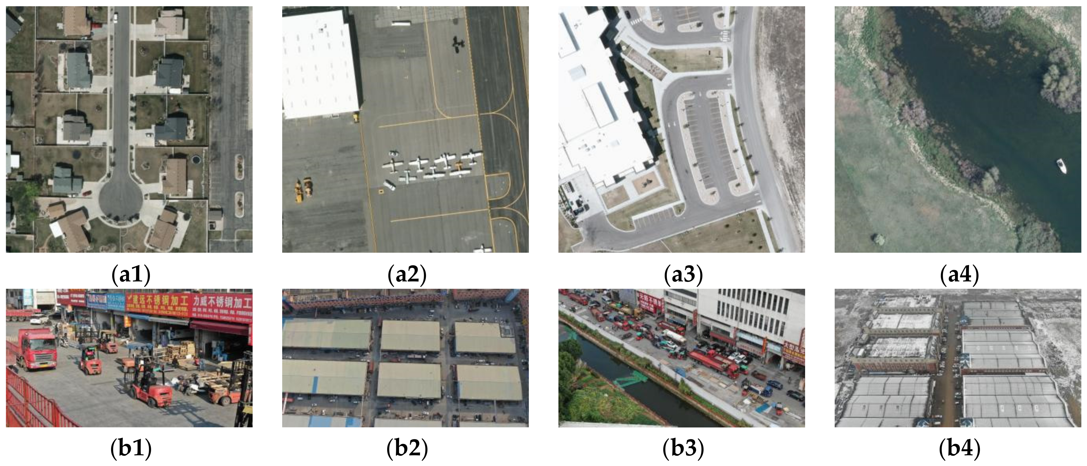
The aerial image of the UAV includes more small targets than the natural image acquired from the horizontal perspective due to the UAV’s flying height and shooting angle. In addition, the objects in the UAV aerial images were arranged in a disorderly manner, with random directions and complex backgrounds. The shortcomings of the present detection methods were described in the preceding section, and they still have a lot of room for improvement. Based on the properties of UAV aerial images, our method aimed to achieve the following goals: (1) enhance the feature extraction capability of the backbone; (2) emphasize important information in UAV aerial images and suppress irrelevant information; (3) increase the receptive field of the detection model; and (4) enhance the target detection ability of the feature pyramid for multi-scale targets. Our improvements mainly concerned the backbone and neck of the model.
2.2.1. Improvement of Detection Model Backbone
Our backbone improvements to YOLOv4 were as follows: (1) choosing more suitable activation functions; (2) applying a new loss function; and (3) adding new attention modules.
(1) Choosing more suitable activation functions.
The activation function was utilized in the detection model to raise the nonlinear factors so that the convolutional neural network was able to approximate any nonlinear function. This allows the model to fully utilize the advantages of multi-layer superposition and improve its expressive capacity. The following two issues must be considered while selecting an activation function: (1) whether it improves gradient propagation; and (2) the cost of function calculation.
Early activation functions include Sigmoid and Tanh activation functions. The functional formula and derivation of the Sigmoid activation function are shown in Equations (1) and (2), and the functional formula and derivation of the Tanh activation function are shown in Equations (3) and (4):
The Sigmoid and Tanh activation functions are smooth and differentiable, and the derivative calculation is convenient. The output of the sigmoid activation function is bounded between 0 and 1, which makes it stable for some larger inputs as well. The output of the Tanh activation function is stable between [−1, 1], symmetric about the 0 center, and the gradient is larger near 0, which is beneficial to distinguish small feature differences. The outputs of the Sigmoid activation function are all positive values, which causes zigzag shaking during gradient descent and in turn reduces the gradient descent speed. The output is not centered at 0, reducing weight update efficiency. Both Sigmoid and Tanh activation functions have nonlinear saturation regions, which easily cause the phenomenon of vanishing gradient during backpropagation. Since the derivative of Sigmoid has a maximum value of 0.25 and the derivative of Tanh has a maximum value of 1, the vanishing gradient of Tanh is slightly smaller than that of Sigmoid.
Since its inception, the ReLU activation function [
40] has become one of the most widely utilized activation functions. The functional formula and derivation of the ReLU activation function are shown in Equations (5) and (6):
Because the ReLU activation function only requires information on whether the input is greater than 0, the calculation is simple and quick. This function converges much faster than the Sigmoid and Tanh functions. The ReLU activation function solves the gradient dispersion problem in the positive interval; however, in the process of back propagation, if the input is negative, the gradient is zero, and there is a Dead ReLU problem. This will cause some units to remain inactivated and the corresponding parameters to never be updated. For the Dead ReLU problem, PReLU [
44], Elu [
45], Leaky ReLU [
41], and other improved methods based on this function were proposed. The functional formulations of the activation functions of PReLU, ELU, and Leaky ReLU are shown in Equations (7)–(9):
The parameter ai in PReLU is usually limited between 0 and 1. If ai = 0, it is converted to a ReLU function; if ai > 0, it is converted to a Leaky ReLU function; if ai is a learnable parameter, it is expressed as a PReLU function. The PReLU, ELU, and Leaky ReLU activation functions all have slopes in the negative domain, thus avoiding the Dead ReLU problem. PReLU requires additional computation and increases the risk of overfitting due to the introduction of additional hyperparameters. Elu involves exponential operations, so the calculation is complicated and slow. Leaky ReLU lacks robustness to noise.
The Swish activation function [
46] is an activation function proposed by Google in 2017. The functional formula and derivation of this activation function are shown in Equations (10) and (11):
The functional formula of the Swish shows that when β = 0, Swish = 0.5x, and when it tends to infinity, Swish is transformed to ReLU, indicating that this function is akin to a smooth function between a linear function and ReLU. Swish is smooth and non-monotonic; the output has lower bounds and no upper bounds; and the effect on deep networks is better than the ReLU activation function. However, its calculation speed is slightly slower than ReLU’s.
The HardSwish activation function [
35] is proposed in MobileNetV3. The functional formulation and derivation of this activation function are shown in Equations (12) and (13):
Compared with Swish, the HardSwish activation function has better stability and a faster calculation speed.
Mish [
36] is the activation function in the YOLOv4 backbone. The functional formulation and derivation of this activation function are shown in Equations (14) and (15):
The Mish activation function improves training stability, average accuracy, and peak accuracy significantly. However, this function is computationally difficult.
In deep networks, especially after layer 16, the accuracy of the ReLU activation function will drop rapidly. The same problem occurs with the Swish activation function after 21 layers. However, the Mish activation function still maintains good accuracy. This small gap is magnified after passing through the deep network, showing a large performance improvement.
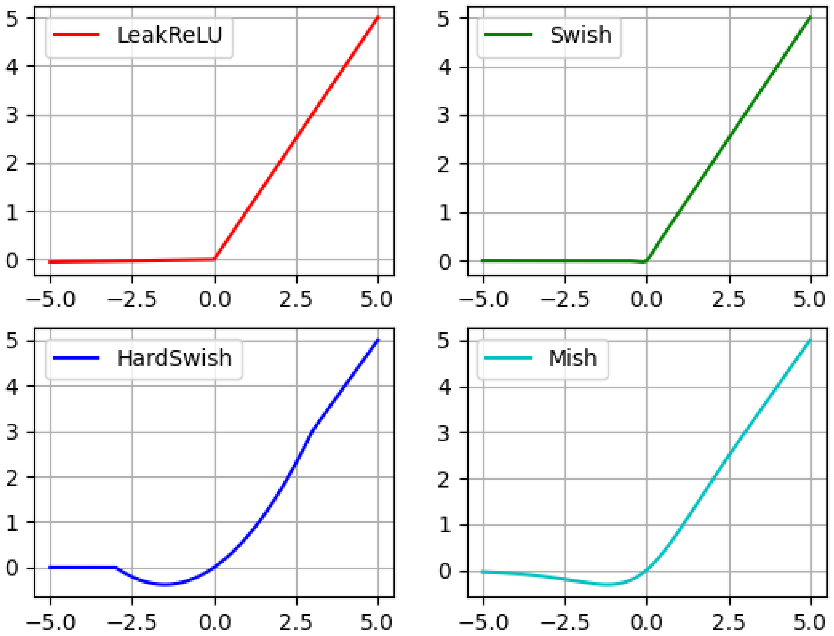
Figure 2 depicts an intuitive comparison of the mathematical models of the Leaky ReLU, Swish, HardSwish, and Mish activation functions, respectively.
In summary, combined with the characteristics of each activation function, we found that the HardSwish activation function has good detection accuracy and computational complexity in shallow networks, while the Mish activation function has a greater contribution in deep networks. Under the trade-off between model complexity and detection accuracy, the activation function in the original YOLOv4 backbone was modified. The activation functions of HardSwish and Mish were used in the first two layers and the last four layers of the backbone, respectively.
(2) Applying a new loss function.
In the YOLOv4 detection method, bounding box regression (BBR) is used to locate objects. The choice of loss function is critical because it can seriously affect the performance of target localization. The early use of the L2 norm loss to compute the loss for bounding box regression [
24,
47], as shown in Equation (16), represents the sum of the squares of the differences between the predicted and ground-truth values. Jiahui Yu et al. [
48] pointed out that the L2 norm loss has two main flaws. First, the correlation between the coordinates of the bounding box is torn, resulting in the inability to obtain an accurate bounding box. Second, the loss is not normalized, so there is an imbalance between objects of different sizes. This causes the model to focus more on large objects while ignoring small objects.
yi is the genuine value, f (xi) is the forecast value, and Ll2 is the loss value in the equation above.
In order to solve these defects, in subsequent research, a loss based on intersection over union (IOU) was proposed. There are mainly IOU loss [
48], GIOU loss [
49], DIOU loss [
50], CIOU loss [
50] and EIOU loss [
37]. Scale invariance, satisfying non-negativity, identity, symmetry, and triangular inequality are all characteristics of IOU, which is a regularly used indicator in object detection. However, if the two bounding boxes do not intersect, the IOU loss cannot accurately reflect the distance between them. Hence, the IOU loss cannot accurately describe the degree of overlap. On the basis of IOU characteristics, GIOU introduces the minimum circumscribed rectangle, which overcomes the problem of the loss value being 0 when the bounding boxes do not overlap. However, when the bounding boxes are contained, GIOU degenerates into IOU. When the bounding boxes are in a state of intersection, the GIOU loss converges slowly in both the horizontal and vertical dimensions. To solve GIOU’s slow convergence speed, DIOU directly returns the straight-line distance between the center points of the bounding boxes, which accelerates the convergence speed. However, the bounding boxes’ aspect ratio is not taken into account in the regression procedure, and the DIOU loss still needs to be improved in terms of accuracy. The CIOU loss adds the loss of length and width to the DIOU loss, which makes the predicted boxes more consistent with the real boxes. However, the aspect ratio in CIOU is a relative value, which is ambiguous. The penalty term of CIOU only reflects the difference in length and width, which may optimize the similarity in an unreasonable way. The EIOU loss is improved following the CIOU loss. EIOU and EIOU loss are calculated using Equations (17) and (18):
The width and height of the minimum circumscribed rectangle covering the ground-truth box and the prediction box are represented by CW and CH in the preceding formula. EIOU loss is divided into the following three parts: IOU loss, distance loss, and location loss. EIOU directly reduces the difference between the width and height of the bounding boxes, which increases the speed of convergence and improves the position effect. YOLOv4 uses CIOU loss when computing bounding box regression. We then replaced it with an EIOU loss.
(3) Adding new attention modules.
The performance of deep convolutional neural networks has been proven to benefit from attention mechanisms. Representative attention modules include the Squeeze-and-Excitation (SE) module [
51], the Convolutional Block Attention Module (CBAM) [
52], and the Efficient Channel Attention (ECA) module [
53], etc.
The SE module improves the feature quality of the network through the interdependence between channels. Through this module, the network can selectively emphasize informative features and suppress irrelevant features. This module is generic and has different effects at different depths throughout the network. Features are excited in a class-independent manner in shallow networks. In deep networks, the module becomes increasingly specialized, responding to different inputs in a highly class-specific manner. The CBAM module computes the attention map along two different dimensions and sequentially, and then multiplies the attention map with the input feature map to obtain the refined features. The ECA module omits the fully connected layer in the SE module and directly performs global average pooling by channels. An adaptive method was then used to determine the number of adjacent channels for each channel, which was proportional to the signal dimension. This method ensured that the module was both efficient and effective.
In the process of determining the weight of each channel, the SE module uses two fully connected layers, which reduces the complexity of the model. However, this procedure seems to be of limited help in capturing the interactions between all channels and thus may be redundant. The channel attention sub-module in the CBAM module adds global maximum pooling on the basis of global average pooling in the past, which enriches the features of the target. However, the CBAM module increases the computational complexity of the module due to the existence of two connected sub-modules. The ECA module avoids the operation of dimensionality reduction and provides an efficient adaptive method to obtain the number of adjacent channels. However, the ECA module only performs the global average pooling operation, ignoring the gain brought by the global maximum pooling.
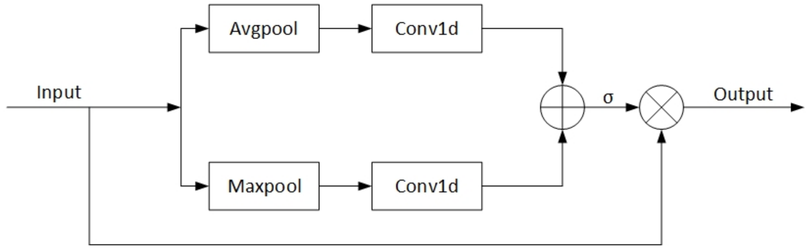
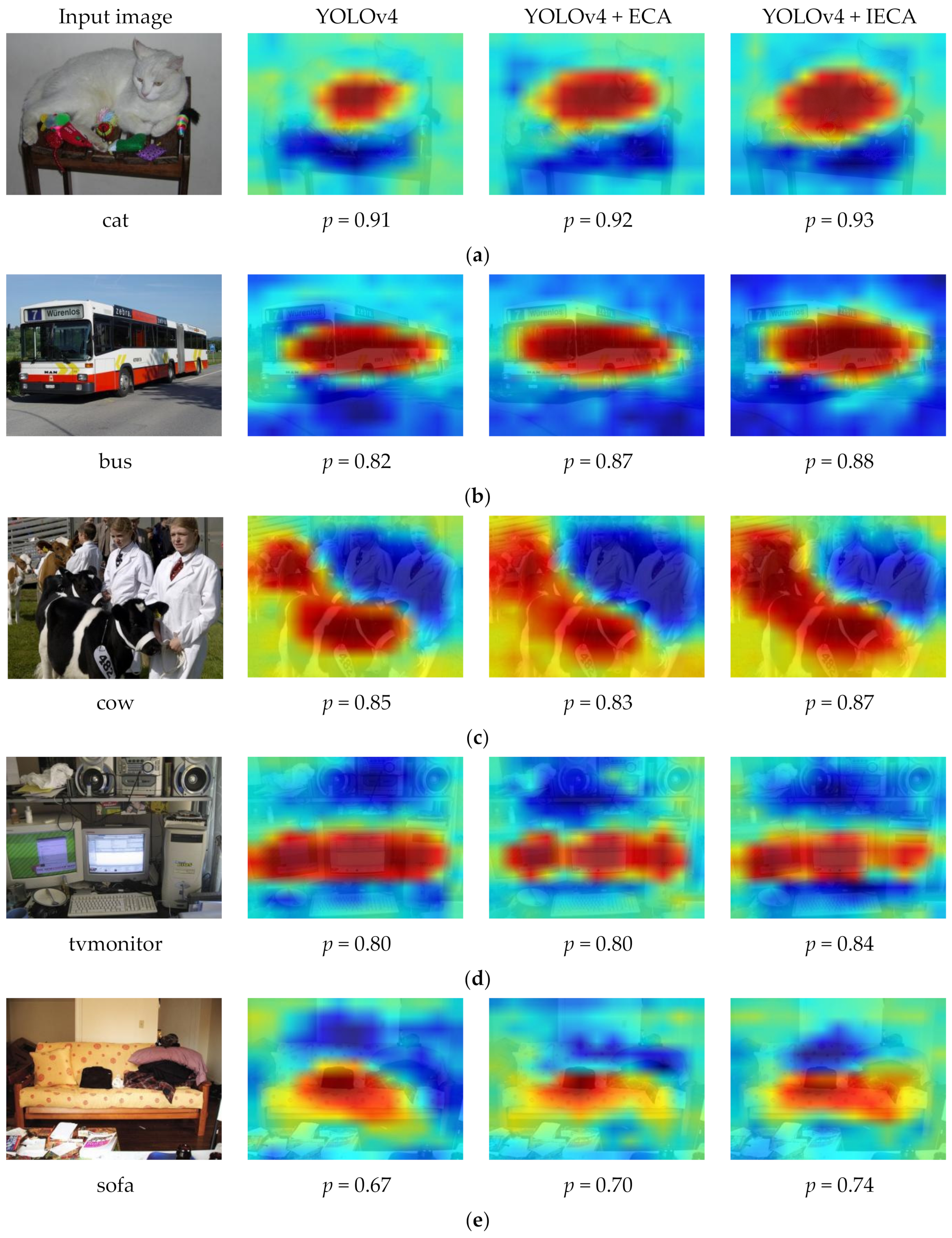
We proposed the Improved Efficient Channel Attention (IECA) module as a new attention module, as shown in
Figure 3. The IECA attention module first utilizes global average pooling and global max pooling operations to obtain channel information for feature maps. Then, the one-dimensional convolution operation is used to adaptively determine the number of adjacent channels for each channel, and the calculated results are added to obtain the attention map of the feature map. Then, the weight of each channel is calculated using the Sigmoid function. Lastly, the final result is generated by multiplying the obtained weights by the input feature map.
2.2.2. Improvement of the Detection Model Neck
Our neck improvements to YOLOv4 were as follows: (1) the pyramid pooling module [
38] was used to replace the SPP module in YOLOv4; and (2) an Adaptive Spatial Feature Fusion (ASFF) module [
39] was added at the end of PANet.
(1) Use the pyramid pooling module to replace the SPP module in YOLOv4.
The SPP module used in the YOLOv4 detection model uses pooling kernels of different sizes to perform a max-pooling operation and then concatenates the individual results. The pooling kernel sizes used are 1, 5, 9, and 13, respectively. Originally, Kaiming He et al. [
54] proposed the SPP module in order to solve the limitation that the CNN must input pictures of a specified size, which avoids the problem of information loss caused by image clipping. Because the proposed SPP module’s output is a one-dimensional matrix, it is unsuitable for the Fully Convolutional Network (FCN), so Joseph Redmon and Ali Farhadi revised it. It was modified as a cascade of max-pooling outputs of different pooling kernels. This structure helps in the expansion of the receptive field and the separation of important contextual features.
The Receptive Field Block (RFB) module [
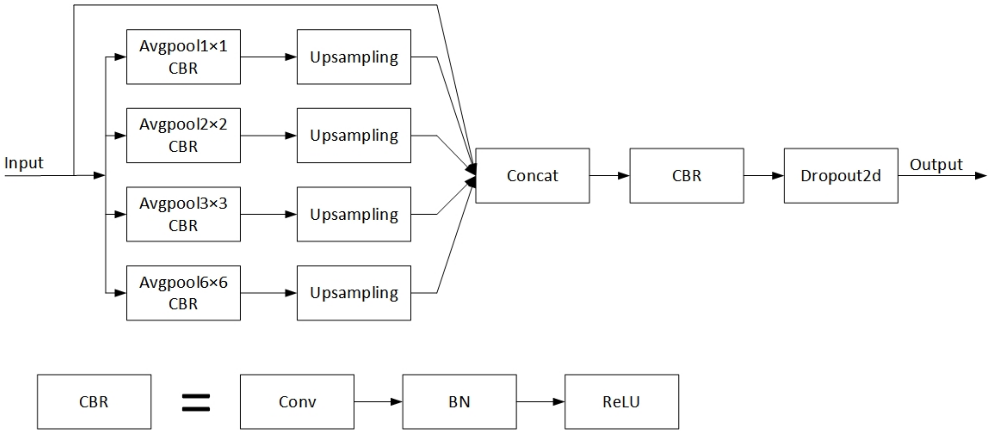
55] and the pyramid pooling module, among others, are employed to increase the model’s receptive field. Songtao Liu et al. proposed the RFB module, which was inspired by the receptive field organization in the human visual system. Multiple convolution branches make up this module, with different-sized convolution kernels providing different-sized receptive fields and dilated convolution providing individual eccentricities for each receptive field. The output of all branches is cascaded at the end, and the final result is obtained by adjusting the number of channels through a convolution operation. The dilated convolutions used in the RFB module are beneficial for expanding the receptive field and capturing multi-scale contextual information. However, they affect the continuity of information and cause local information loss. In addition, since dilated convolutions sparsely sample the input signal, there is a lack of correlation between the information obtained by long-distance convolution. The Pyramid Scene Parsing Network (PSPNet) uses the pyramid pooling module to generate feature maps of various sizes. This module contains operations for average pooling with various strides and output sizes. Bilinear interpolation is utilized to adapt each feature map to the same size during the operation, and then all feature maps are stacked. The pyramid pooling module comprises four different scales of features, which are separated into 1 × 1, 2 × 2, 3 × 3 and 6 × 6 sub-regions in sequence from coarse to fine. This helps to fully utilize each region’s contextual information, resulting in more accurate prediction results.
Figure 4 shows the pyramid pool module’s architecture.
In our experiments, we found that replacing the SPP module in YOLOv4 with the pyramid pooling module improved the distinguishing and robustness of features and obtained more reliable prediction results.
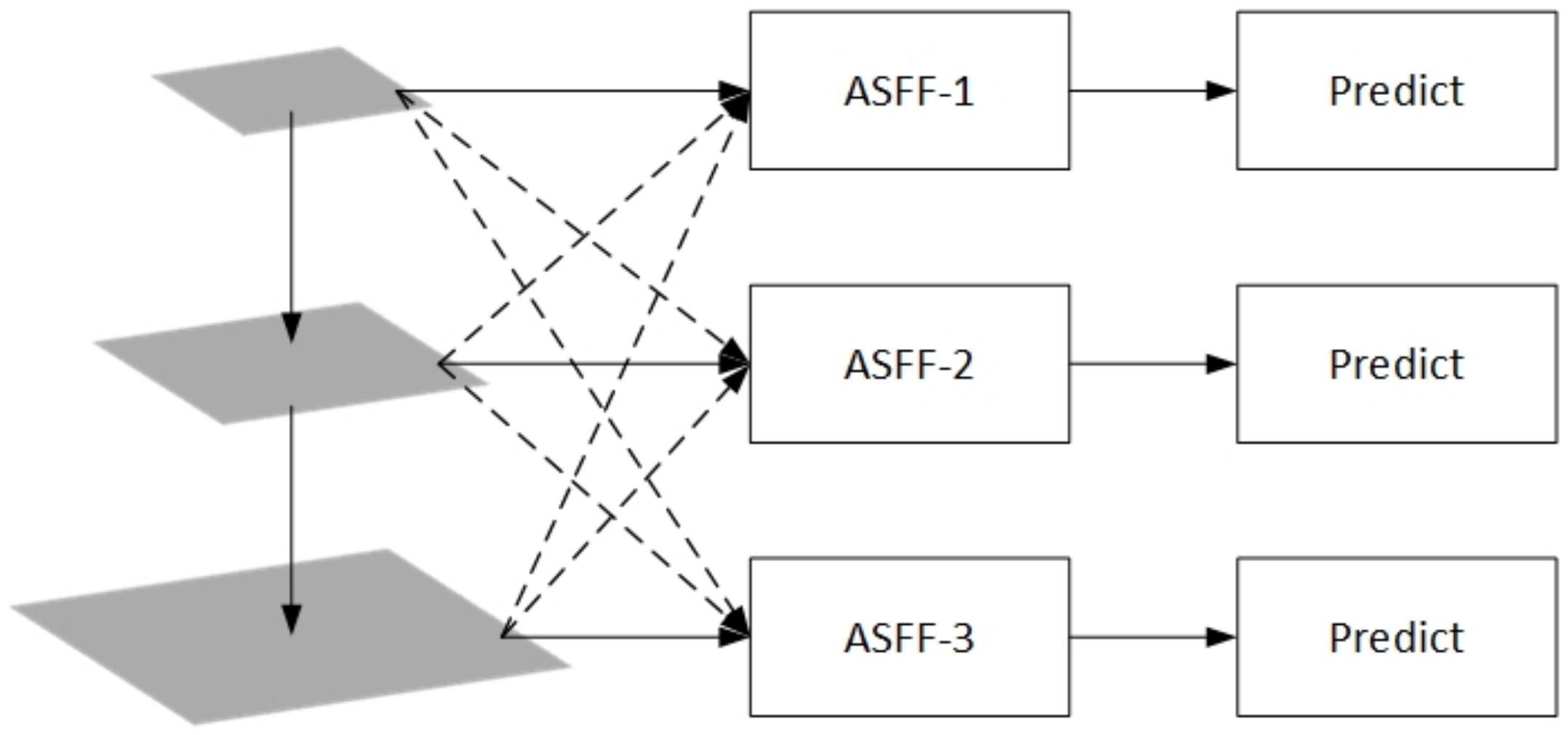
(2) An Adaptive Spatial Feature Fusion (ASFF) module at the end of PANet was added.
Pyramid-shaped feature representations are often used to address the challenges posed by scale changes in object detection. However, when using feature pyramids to detect objects, inconsistencies between different feature scales can cause unnecessary conflicts. For example, YOLOv4 detects small and large objects using feature maps of sizes 52 × 52 and 13 × 13, respectively, when the input image resolution is 416 × 416. If an image contains objects of different sizes at the same time, the small object will be regarded as the target on the 52 × 52 feature map, but it will be regarded as the background on the 13 × 13 feature map. The same is true for large objects. The ASFF module is used to address the inconsistency of feature pyramid characteristics in one-stage detectors. This module retains useful information from each feature map and combines them by filtering feature maps of different sizes. The ASFF module first resizes all feature maps to the same size, and then finds the optimal feature fusion method during model training. At each spatial location, feature maps of different sizes will be adaptively fused to filter out the contradictory information carried by the location and to retain those more discriminative clues. As shown in
Figure 5, we added this module at the end of the neck of the YOLOv4 model, which promoted feature extraction and increased the model’s detection accuracy.
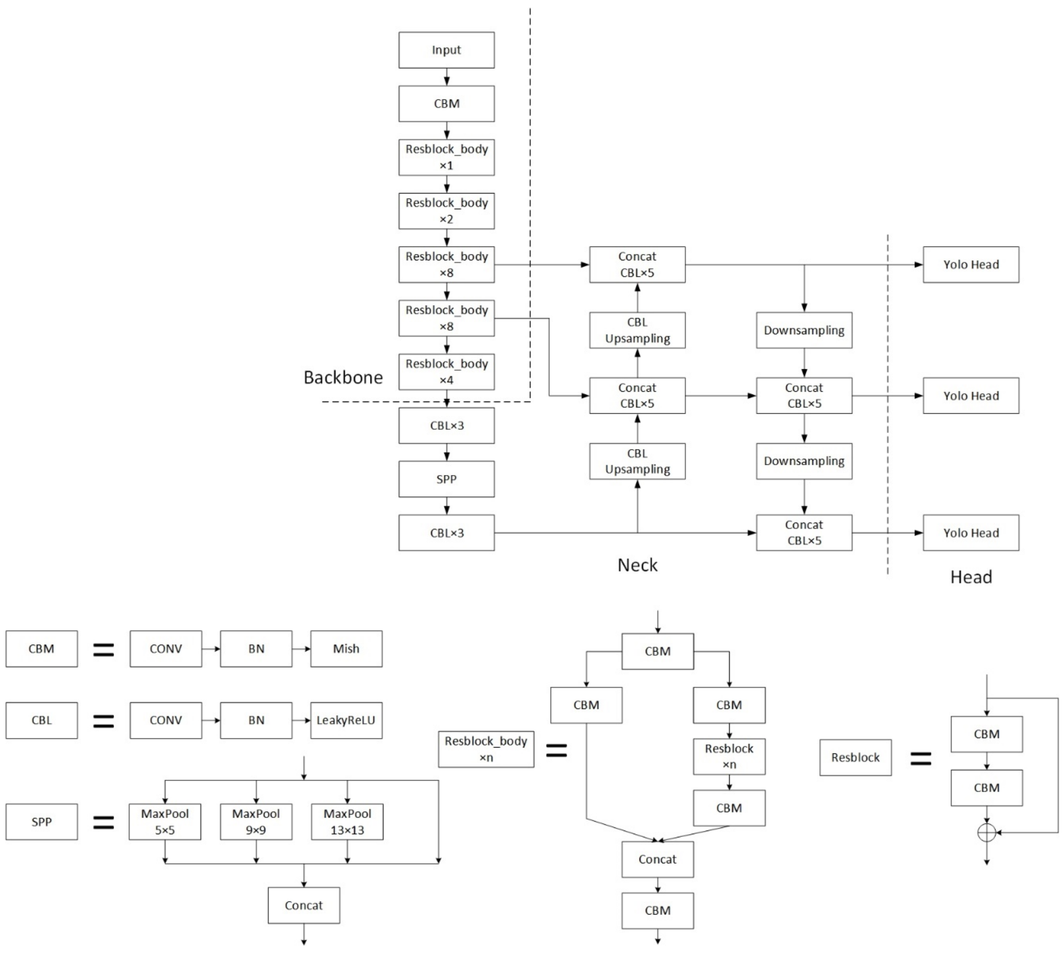
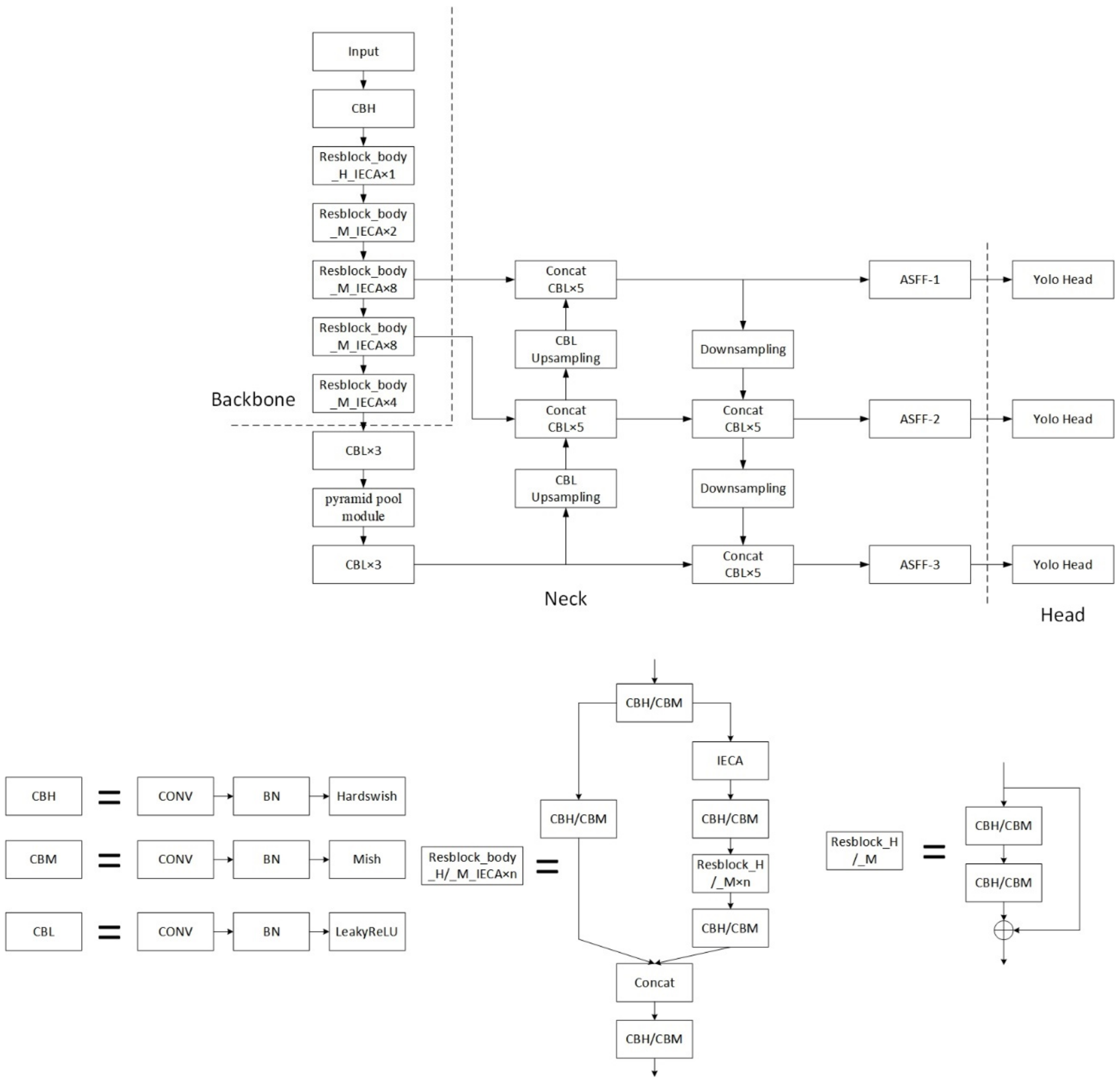
In summary, we made some improvements on the basis of the YOLOv4 model, replaced some modules in the original model, and added some new modules. The architecture of YOLOD is shown in
Figure 6. When the input UAV aerial imagery is 416 × 416 pixels in size, it first passes through the backbone to produce three feature maps with sizes of 52 × 52, 26 × 26, and 13 × 13, respectively. Then, the feature maps extracted by the backbone undergo feature fusion through the neck to deepen the feature extraction. Finally, the model’s head outputs the final forecast result.


