
Operational Use of EO Data for National Land Cover Official Statistics in Lesotho


1
Office of the Chief Statistician, Food and Agriculture Organization of United Nations, 00153 Rome, Italy
2
FAOLS, Maseru 7588, Lesotho
*
Author to whom correspondence should be addressed.
Remote Sens. 2022, 14(14), 3294; https://0-doi-org.brum.beds.ac.uk/10.3390/rs14143294
Submission received: 1 June 2022
/
Revised: 27 June 2022
/
Accepted: 4 July 2022
/
Published: 8 July 2022
(This article belongs to the Special Issue Advances in Satellite-Based Land Cover Mapping and Monitoring)
Abstract
:The Food and Agriculture Organization of the United Nations (FAO) is building a land cover monitoring system in Lesotho in support of ReNOKA (‘we are a river’), the national program for integrated catchment management led by the Government of Lesotho. The aim of the system is to deliver land cover products at a national level on an annual basis that can be used for global reporting of official land cover statistics and to inform appropriate land restoration policies. This paper presents an innovative methodology that has allowed the production of five standardized annual land cover maps (2017–2021) using only a single in situ dataset gathered in the field for the reference year, 2021. A total of 10 land cover classes are represented in the maps, including specific features, such as gullies, which are under close monitoring. The mapping approach developed includes the following: (i) the automatic generation of training and validation datasets for each reporting year from a single in situ dataset; (ii) the use of a Random Forest Classifier combined with postprocessing and harmonization steps to produce the five standardized annual land cover maps; (iii) the construction of confusion matrixes to assess the classification accuracy of the estimates and their stability over time to ensure estimates’ consistency. Results show that the error-adjusted overall accuracy of the five maps ranges from 87% (2021) to 83% (2017). The aim of this work is to demonstrate a suitable solution for operational land cover mapping that can cope with the scarcity of in situ data, which is a common challenge in almost every developing country.
1. Introduction
Land Cover (LC) maps can be used to extract key information for a series of national applications, such as environmental monitoring, identification of land degradation trends, spatial planning, and for a wide range of scientific research fields. However, continuous monitoring and reporting of land cover maps requires regular updating, the use of standardized methods, and the adoption of a robust validation framework ensuring that every estimate is accurate and consistent over time. Such land cover mapping solutions are very rare to find in countries due to the inherent technical and financial challenges found in both traditional and modern LC mapping methods.
The most traditional methods that have been typically used in the last two decades have been based, initially, on visual image interpretation and pixel (or object) classification, relying on the use of very high-resolution images (commercial satellite images and ortho-photos), and subsequently, on the combination of Earth Observations and in situ data for calibration and validation of automatic classification models. Such solutions have been extensively used in the research community [1,2,3,4].
FAO adopted a visual interpretation approach in 2015 to deliver the first edition of the Lesotho Land Cover Atlas [5]. The methodology relied on a manual labeling of segmented objects from very high-resolution preprocessed satellite imagery using a visual image interpretation. Preprocessing of the satellite imagery included pen-sharpening of Rapid Eye 2014 single date imagery with ortho-photos collected in 2014. The resulting cloud-free mosaic, at 1.5 m/2 m spatial resolution, was then subjected to segmentation using the E-Cognition proprietary algorithm [6]. A collection of nearly 1 million polygons was derived and divided into nine tiles, which were assigned to a group of 30 dedicated image interpreters. Each polygon was visually interpreted and assigned to one of the 32 level-II land cover classes, which had been defined following the FAO Land Cover Classification System (LCCS) system. While this mapping approach was crucial to establish the first national baseline, it could not be replicated easily as it is resource intensive—outputs are delivered with a significant time lag and introduce subjectivity in the object classification.
After 2015, with the advent of free high-resolution satellite imagery from the Sentinel fleet operated by the Copernicus program of the European Union, together with the availability of a low-cost cloud computing facility and rich machine learning libraries, it is now possible to carry out land cover mapping in a much more cost-efficient way by integrating Machine Learning (ML) and Open Access Geospatial Data [7]. The short revisit period of Sentinel-1 and Sentinel-2 images (4 to 5 days) has allowed for developing land cover mapping approaches based on dense time series as opposed to monotemporal image analysis; this has increased the capacity of classifiers to better discriminate vegetation types with positive impacts on the overall accuracy of results. Studies have been conducted on mapping land cover in different areas of the world including Europe, Africa, and Asia, using optical data alone (Sentinel-2) or a combination of optical and SAR data (Sentinel-2 and Sentinel-1) [8,9,10,11].
Despite the proliferation of these new approaches, all supervised classification algorithms remain dependent on the utilization of a sufficiently large set of representative training samples to generate accurate land cover maps. The quality of land cover maps, typically measured with accuracy statistics derived from the confusion matrix [12], depends on the quality of the in-situ dataset, its accurate geographical positioning, its spectral consistency, and the representativeness of the dataset of the full range of land cover conditions in the field. However, in situ data of adequate quality and sufficient quantity are rarely available in countries, due to the high costs and logistic problems associated with the collection of these data on a large scale on a regular basis. The lack of in situ data poses a major challenge to the establishment of an efficient and sustainable land cover mapping solution at the national level and is an important limiting factor for the uptake of EO methods by National Statistics Offices in the production of official land cover statistics [13,14].
In response to these issues, alternative solutions for the collection of field data for the purpose of land cover mapping have been developed by using training data, extracted, for instance, from the visual interpretation of satellite images [15,16]. Despite this approach being more practical than the implementation of field surveys, it is still time-consuming and subject to the introduction of classification errors due to the subjective nature of the interpretation by the operator. Alternatively, training data can be extracted from existing land cover maps. The Climate Change Initiative Global Land Cover (CCI_LC) dataset, produced by the European Space Agency (ESA, Paris, France), was used to extract the spatial–temporal spectral signature of each land-cover type, and subsequently, to classify Landsat Operational Land Imager (OLI) data, producing a land cover map of China [17]. Samples were extracted from the National Agricultural Statistics Service (NASS, Washington, DC, USA) Cropland Data Layer (CDL) dataset [18] and used as training data to produce the 2011 National Land Cover Database (NLCD) product [19]. Samples extracted from the Moderate Resolution Imaging Spectroradiometer (MODIS) (NASA, Washington, DC, USA) land cover products (MCD12Q1.006) were used to train a random forest algorithm to produce a land cover map in an area of northern China by classifying LandSat time series data using Google Earth Engine [20].
Costa et al. (2018) [21] proposed a general framework for routine monitoring and statistical reporting of land cover and land cover change in Portugal using training pixels extracted from Google street view and ortho-photo maps; in this paper, Landsat images were interpreted using a combination of three machine learning classifiers (ANN, RF, and SVM). Cong Lin et al. (2019) [22] applied a knowledge transfer technique to transfer label information from the Globeland30 global dataset and map the rapidly urbanizing region within the Yangtze River Delta city cluster in China.
Even though training data extracted from existing land cover products are a potentially useful source of information, their application is still not straightforward. Such data are not fully reliable since they may embed classification errors, inherited by the source land cover product, due to both misclassification errors in the original product and land cover changes linked to the different timings of extraction of the pixel imageries. Furthermore, training data are usually aggregated at the polygon level, which often include heterogeneous areas and result in spectral inconsistency of the object. Lastly, there may be a semantic gap between map legends and Remote Sensing (RS) data [17].
Several approaches have been developed to curate the training data to ensure positional and spectral quality. For example, when a time series of LC maps is available, pixels, which do not change land cover class over a period of three years, are selected [23]. Additionally, training data can be sampled so that the LC class proportions of the training dataset are representative of the population they were extracted from. In 2020, Paris and Bruzzone developed a novel approach for the unsupervised extraction of reliable training samples from thematic products [24], which ensures the spectral coherence of the training data and is better suited to automatize the imagery interpretation process.
In order to solve the fundamental challenge of the lack of in situ data of adequate quality, which is hindering the establishment of operational land cover mapping systems in countries, in 2021, FAO developed a new methodology that was tested in Lesotho under the auspices of the national Integrated Catchment Management (ICM) program implemented by the Government of Lesotho and funded by a multi donor consortium (comprising the European Union, the Deutsche Gesellschaft für Internationale Zusammenarbeit (GIZ), and the Government of Lesotho).
The solution named EOSTAT Land Cover Mapper, is provided free of cost and is currently hosted on Google Earth Engine. The codes developed by FAO can be accessed in the Supplementary Materials section.
The solution has the following characteristics:
- It allows for the production of next-generation standardized annual land cover maps;
- It copes with the lack of in situ data and the limited resources available in most countries for the collection of training and validation data;
- It is provided free of operating costs;
- It is user friendly and can be easily operated by national staff.
The paper is structured with the following sections: (i) Introduction, where, after providing background information on the country project implemented in Lesotho, the main methods for large-scale land cover mapping and for gathering in situ data are described; (ii) Data, where the definition of a machine-learning-friendly legend, using FAO LCCS, the production of Sentinel-2 Analysis Ready Data cubes, and the available in situ data for the baseline are presented; (iii) Methods, where the automatic generation of in situ data using K-means, the use of Random Forest for the classification of the national land cover maps, and the framework for the accuracy analysis of the annual land cover estimates and their consistency over time are reported; (iv) and (v) Main Results and Discussion, where the final outputs are presented and areas for possible enhancement of the method for the automatic generation of training data are described; (vi) Conclusions, which summarize the most important takeaways from the paper.
2. Data
2.1. Study Area
The study area is the territory of the Kingdom of Lesotho (Figure 1), which is a landlocked country, surrounded by South Africa (Figure 1a). The total area of the country is 30,450 km2, ranking as the 137th largest country on the planet. Lesotho’s territory is covered by 7 Sentinel-2 Tiles (Figure 1b).
Lesotho’s population was estimated to be 2.176 million in 2022 by the UN Population Division and is expected to grow to 2.325 million by 2030 and 2.665 million by 2050 [25]. Poverty rates are very high, with 62 percent of the population of Lesotho living on less than 2 USD per day and 36.4 percent on less than 1 USD per day. The main economic sector in Lesotho is agriculture, which, in 2019, provided work and income to 44.3% of the country’s total employment.
Lesotho is climatically characterized by two main seasons: a rainy season from October to the end of March and a dry season from April to the end of September. Typically, most of the precipitation occurs during the southern hemisphere summer thunderstorms. Lesotho’s territory is divided into four agroecological zones—the lowlands, foothills, Senqu River Valley (SRV), and mountains [26]—which are characterized by four different lengths of growing period (LGP) based on analysis of climate, soil, and terrain data (Figure 1b). Agroecological zones (AEZs) are homogeneous ecosystems that influence plant phenology dynamics, including photosynthesis (plant chlorophyll content) [27]. AEZs are a very important aspect for the study, specifically for the stratification of the in situ data survey design and the reference data curation procedure.
2.2. Definition of Land Cover Legend (LCL)
Definition of the land cover legend (LCL) is a critical step in a land cover mapping project as it provides a method to express the thematic content of a map that can be easily interpreted by different users. The legend reflects how the semantic “generalization” of a specific geographic area has been conceived. The process of categorization is therefore meant to minimize the complexity of the real world, where different area types are in fact distributed on a “continuum”. Since the definition of classes is, by nature, an arbitrary process, it may lead to uncertainties that will deeply affect the accuracy of the final land cover map. Therefore, it is important that the definition of the LCL assures two minimum requirements [28]:
- Clear and unambiguous class definition.
- No class semantic fuzziness. Class (semantic) boundary not overlapping with other legend classes.
In line with such recommendations, the LCL developed during the production of the Lesotho Land Cover Database 2015 was initially reviewed for potential reuse. The LCL 2015 contained 32 level-II land cover categories, as shown in Table 1, which were defined using FAO’s ISO 19144 Land Cover Meta Language [29]. The 32 level-II classes were grouped under six level-I classes.
A number of land cover classes contained in the LCL 2015 were identified as spectrally heterogeneous and affected by a fuzzy definition. Such classes, listed in Table 2, included those defined as “open”, plus those named “Trees Undifferentiated”, “Trees sparse”, “Rural Settlement Plain Areas”, and “Rural Settlement Sloping Areas”. Such classes included a combination of one pure land cover feature mixed with one or more different land-cover-type features.
“Open” classes were considered unsuitable for inclusion into a multiclass machine learning classifier due to their lack of spectral homogeneity. Spectral homogeneity of training data is a prerequisite for machine learning classification, especially in pixel-based approaches, as it ensures low intraclass spectral variability (i.e., all pixels within that class are similar to each other) and maximum interclass differentiation (the pixels within one class look very different from pixels from other classes). When “open” land cover classes, or more generally, fuzzy classes are used in a land cover legend, this inevitably introduces mixed pixels in the training dataset, which belong to the same class but have very different spectral values. This introduces noise and hampers the capacity of the classifier to discriminate correctly between land cover classes. For this reason, land cover classes affected by a fuzzy and heterogeneous spectral profile were eliminated from the legend to produce the new land cover database. Table 2 summarizes the list of these classes and their respective spatial extent (pixel count and km2). They amount to nearly 19% of Lesotho’s total land area, with the vast majority being Shrubland (open).
Moreover, the following classes were merged due to their overlapping class definitions to minimize fuzziness between classes:
- Plain (HCP) and slopes (HCSM) croplands merged as (Rainfed) Cropland. The crop phenology between plain and slopes croplands is not sufficiently different to be able to discriminate between the two in a reliable way.
- Urban (UA1), Industrial (UA2), rural (RH1), rural (RH2) settlements as Built-up. A machine learning classifier focuses on the classification of built-up and impervious surfaces rather than the spatial layout of what constitutes an urban/industrial or rural settlement.
- Bare Rock (BR), Bare Area (BA), and Boulders and Rocks (BLR) as Bare Surfaces. Different bare surfaces exhibiting absence of photosynthetic activities are hard to distinguish from one another using multispectral imagery.
- Small (WB1) and Big (WB2) Water Bodies merged as a single Water class. If water body size is an information of concern, it can always be retrieved a posteriori.
- Trees—Needle-leaved (closed) TNL2, Trees—Broad-leaved (closed) TBL2, Trees—Undifferentiated (closed) TM1, merged as a single Trees class. Trees in Lesotho are not an abundant class (3.5% of surface area), and the existing surveys that distinguished between needle-leaved and broad-leaved trees were not accurate enough to assist field sampling of sufficient in situ samples for mapping them as separate classes.
Final amendments included the elimination of three classes that were considered to be straying away from the concept of land cover:
- (i)
- “Rainfed agriculture Sheet erosion”, as it included both cropland and bare soil; hence, it was considered an “open” class.
- (ii)
- “Grassland degraded”, as it contained both grassland and bare soil and shrubs.
- (iii)
- “Shrubland degraded”, as it included shrubs and bare soil.
Indeed, the above classes integrate the concept of degradation, which is not easily combined with land cover. Land cover describes the dominant surface in the landscape, while degradation describes the status of that surface. Land degradation status is better assessed using time-series methods relying on land cover data as a stratification layer rather than embedding “degraded” classes in the nomenclature.
2.3. Sentinel-2 Analysis Ready Data (ARD) Cubes
Sentinel-2 bottom of atmosphere (BOA) images were preprocessed and transformed into five Analysis Ready Data cubes, one for each land cover reporting year (from 2017 to 2021). Sentinel-2 images were acquired from 1 September of the previous year through to 31 August of the reporting year. Production of the ARD’s involved (i) the masking of clouds and cloud shadows using the s2cloudless Sentinel-2 cloud probability and (ii) the bimonthly temporal aggregation using the geometric median [30] of the cloud-masked images, resulting in six cloud-free temporal composites for each reporting year.
Figure 2a displays the NDVI calculated from the Sentinel-2 time series for the reference year, 2020, after cloud masking was applied. Gaps are evident for several dates. Figure 2b shows the NDVI calculated and interpolated from the temporal aggregation of the Sentinel-2 cloud masked data series for the same reference year. It can be seen how the NDVI data points for each object are harmonized, and the signatures are still perfectly distinguishable.
Use of temporal aggregation is always a recommended practice, as it leads to the reduction of data size and the preservation of cloud-free observations at key phenological stages of the year. However, it should be noted that some data gaps may remain in the temporal composites in cases of heavy cloud coverage at specific times of the year. Nevertheless, a Random Forest classifier can handle some data gaps through median imputation or proximity-based measure. A longer time interval could have been chosen to reduce the occurrence of gaps in the ARD time-series, but this would have further averaged out and blurred the temporal signature of the observed land cover classes. Inversely, if a shorter time interval were chosen to obtain a finer-grained temporal signatures of the observed land cover classes, it would have resulted in larger data gaps in the ARD time-series. For these reasons, a 60-day temporal interval was deemed to offer the right compromise between data gaps and detail of the temporal signature for Lesotho. A different length of temporal aggregation may be more suitable for other geographic locations.
As a result, the ARD’s contained all the 10 m and 20 m bands from Sentinel-2, as shown in Table 4, plus the NDVI and EVI indexes.
2.4. In Situ Data
An ad hoc field survey was designed and implemented to gather in situ data for the purpose of developing a baseline land cover map for the reference year, 2021. This step was of paramount importance for the success of the project, as it provided the foundation data layer for establishing an accurate and validated land cover baseline for the reference year, 2021, on one side, and on the other side, to allow for the automatic production of training data required to compute the annual land cover maps for the other years (2017 through 2020) for which no in situ data were available.
A total of 2800 land cover georeferenced data samples were gathered through the field survey. This sample size was considered optimal, based on available survey resources and in line with the requirements from best practices [31] in validation of remote sensing products. Such practices consider two criteria: (i) the number of classes; (ii) the size of the land cover map, as shown in Table 5.
A stratified multistage sampling strategy was adopted for the scope of geographically distributing the sample spots in an optimal way. The landscape of Lesotho was first divided into four strata based on the AEZ and then further intersected with the districts’ boundaries: as a result, a collection of 25 subdistricts was obtained, as shown in Figure 3.
Each subdistrict was used as a Primary Sampling Unit (PSU). A probabilistic approach was used to calculate the number of samples to be collected per each land cover class within each PSU (see Table 6 for a summary by district). The probabilistic sampling approach ensured that each land cover class would be sampled proportionally to its relative number. The following Formula (1) was used:
where
- is the total number of samples allocated to LC1 within subdistrict 1;
- is the area (km2) covered by LC1 subdistrict 1;
- is the area (km2) covered by LC1 within Lesotho national territory;
- is the total number of samples to be collected by the survey.
An inflating factor of +10% was introduced for three minor classes (irrigated crops, wetlands, and dongas) to ensure a sufficient number of training data for the classifier. This sampling design increases the fraction of samples taken within the stratum where the rarely occurring cases are concentrated.
As a final step of the field survey, the spatial allocation of sampling sites within the 25 strata was determined to ensure the accessibility of the locations to the survey team. Primary, secondary, and tertiary road segments of Lesotho extracted from the Open Street Map (OSM) layer were buffered using three bandwidths (200 m, 150 m, and 60 m, respectively). The buffers were intersected with the 25 subdistricts and with the land cover 2015 data. The intersecting polygons were finally used as target areas and the sampling sites were randomly generated within these (Figure 4a,b).
As a result, a total of 3581 samples were collected as reported in Table 6.
The in-situ dataset was quality controlled to ensure positional accuracy and consistency of attributes. The final dataset containing 3581 samples was further split into two subsets: one for training (80% of total samples) and one for validation (20% of total samples).
3. Methodology
The production of Next-Generation Land Cover database relied on a state-of-the-art statistical and machine learning approach, substantially different from the initial methodology used in 2015. The availability of new cloud computing infrastructures, such as the Google Earth Engine, and the availability of the Sentinel-2 data archive allowed for the land cover mapping production process to be automatized while improving the accuracy and consistency of these products. Some of the most significant differences are listed in Table 7.
The new land cover mapping methodology was organized in 4 main steps, as shown in Figure 5:
- In Step I, the land cover training and validation dataset was created or, if already available from the previous year, it was updated to the new reference year.
- In Step II, Sentinel 2 data were preprocessed and transformed into Analysis Ready Data (ARD), also called Data Cubes.
- In Step III, the land cover classification was performed, using a supervised classifier (Random forest), producing annual land cover maps.
- In Step IV, the validation of annual land cover maps was performed.
3.1. Step I: Automatic Reference Data Sourcing
Land Cover reference data, also known as “ground truth” or “in situ” data, are required to train a land cover classifier (e.g., random forest) and to validate the accuracy of the resulting land cover map. Reference data are traditionally collected in the field through GPS-assisted field surveys. Such reference data are required to be representative of all the land cover classes within all of the different agroecological conditions and should reflect the situation on the ground for the same reporting period of the mapping exercise. Keeping reference data up to date within the context of operational land cover mapping is crucial to ensure map accuracy. However, this is a very difficult task to achieve through traditional field surveys due to the very high costs and time requirements associated. In this context, an innovative solution was developed allowing for the automatic generation of pseudo in situ training and validation datasets for any given reference year that is within a time span of 5 years from an existing baseline. The assumption is that a land cover map and/or an in situ dataset for the baseline year is/are available. In the context of the Lesotho mapping exercise, in situ baseline data were gathered in 2021 (as described in Section 2.4), and a baseline land cover map for 2021 was also produced. Both were used as baseline data to automatically produce validation and training datasets for the years 2017, 2018, 2019, and 2020. A time window of 5 years was selected for the generation of training data to match the initial availability of a sufficient number of tiles of Sentinel-2 data for Lesotho, which started in 2017.
The automatic production of reference data included two key modules:
- Within-class K-means clustering, using the 2021 land cover data as stratification layer. The 2021 land cover map was used jointly with the Sentinel-2 ARD cube prepared for a target year (as described in Section 2.3) to train a stratified K-means clustering algorithm. For each land cover class, 15–30 NDVI clusters were generated using as input the Sentinel-2 bimonthly composite (November–December) corresponding to the vegetation peak: the exact number was determined using the Calinski–Harabasz Index [32]. The reason for determining a large range for the cluster number is to produce enough small clusters, which could be associated to outliers. The goal of this step is to isolate the “purest” and most representative pixels of each class in a set of clusters, while allocating the remaining pixels to outlier clusters (Figure 6).
- Clusters sampling using the baseline reference dataset from 2021. The 2021 in situ reference dataset for each land cover class was used to sample from the generated clusters. For clusters that corresponded to less than 5% of the given land cover class sample abundance, those samples were trimmed. The assumption is that if a minority of points (<5%) falls inside a given cluster, this cluster is an outlier to the land cover class and should be omitted. This assumption holds if the baseline reference data are from a high-quality, balanced reference dataset, i.e., it maximizes intraclass variability and interclass separability for the given geographic area. Such an approach incurs the risk of removing perfectly valid data points, but by keeping the threshold low (5%) and the number of clusters high (15–30), the risk is minimized.
Figure 6.
The K-means clustering decomposition of a cropland object extracted from the LC 2021 (object includes cropland, built-up, and water as shown by the background very high-resolution image. While cropland largely dominates (19 “green” samples in cropland), built-up and water are identified as minority clusters (red dots, 1 in built-up and 1 in water); pixels within these are outliers and are removed. As a result, four in situ datasets were generated, one for each reference year, as shown in Table 8. The original number of training pixels in the baseline dataset 2021 (3581) was eroded by an average −2.7% per year, as a result of each iteration of the k-means and outlier removal routine. For instance, for the year 2020, 3260 pixels were retained (−321 pixels). The year 2017 contained 3166 pixels (−415). Therefore, it is advisable to collect ground truth data to conflate the cleaned-up dataset every 5+ years, depending on the rate of decay of the dataset). Built-up and Water clusters are minor clusters and are eliminated by the filtering process, which keeps the dominant cluster that represents cropland.

The curated in situ annual datasets were further split into training and validation sub datasets using the proportions 70/30%, as shown in Table 9.
3.2. Step II: On-2.5.2 On-the-Fly Generation of Sentinel 2 ARD Cubes
This step is described in Section 2.3, as it pertains to the preprocessing of input data. However, for consistency of the narrative on the methodology, it is important to recall its relevance about step II.
3.3. Step III: Production of Next-Gen Annual Land Cover Maps
A supervised classification of land cover was performed using a Random Forest (RF) approach for every reporting year from 2021 back to 2017, using as training data the reference datasets (Table 8 and Table 9).
3.3.1. Production of the Next-Gen Annual Land Cover Map for the Reference Year 2021
A Random Forest (RF) classifier was trained in Google Earth Engine (GEE) using the reference dataset 2021 (Table 8). The in-situ dataset was split into a training and a validation dataset following an 80%/20% split (Table 9). The distribution of samples per land cover class was determined via a probabilistic sampling based on class area abundance, jointly with inflation of sampling of minor classes, as described in Section 2.4. The distribution of training samples per LC class is shown in Figure 7.
Spectral values from all bands, plus NDVI, were extracted from the Sentinel-2 ARD data cube 2021. The hyperparameters chosen for the random forest implementation were the following:
- -
- 50 trees;
- -
- 1 Minimum Leaf Population;
- -
- 50% bagging fraction;
- -
- Unlimited maximum nodes.
3.3.2. Production of the National Land Cover Maps for the Reporting Years 2017, 2018, 2019, and 2020
The training datasets (Table 9) and the Sentinel-2 ARD cubes for the years 2017, 2018, 2019, and 2020 were used to train the RF and to predict annual land cover maps for the reporting years from 2017 through 2020. Likewise, for the production of the land cover map 2021, the Sentinel 2 bands and NDVI were used as predictor features. Parametrization of the RF was standardized across the time series and used the same setting as that used to produce the land cover map 2021. As a result of this step, a time series of 4 annual land cover maps was produced for the period 2017–2020.
3.4. Postprocessing and Harmonization
The land cover maps produced for the entire period were postprocessed to (i) eliminate artifacts (e.g., salt and pepper effects); (ii) ensure thematic consistency (e.g., removal of water over steep slopes); (iii) filter out seasonal changes of land cover and unlikely land cover changes; and (iv) to map features that do not fit the standard procedure described above (e.g., Gullies, Irrigated Cropland). The harmonization procedure was based on consistency analysis at pixel level using a three-year time window in line with the methodology used for the development of the ESA CCI [33].
Two rules were implemented:
- If pixel in the second year is different from previous and following year, and the previous and following year belong to the same LC class, the middle pixel is converted to that class. This is applied to all classes apart from the water class, which is allowed to fluctuate on an annual basis (water levels in the dam are likely to fluctuate annually).
- The following impossible or unlikely transitions have been disallowed for a period of 3 consecutive years (beyond 3 consecutive years, these transitions are allowed again, as it is undesirable to enforce harmonization rules indefinitely):
- ○
- Water to Built-Up;
- ○
- Built-up to Cropland;
- ○
- Bare Soil to Cropland;
- ○
- Built-Up to Bare Soil;
- ○
- Any class to Forest aside from Wetland and Shrubland;
- ○
- Any class to Wetland aside from Grassland, Shrubland, and Cropland;
- ○
- Any class to Shrubland aside from Wetland, Grassland, and Forest;
- ○
- Any class to Grassland aside from Bare Soil, Cropland, and Wetland.
The postprocessing included the following rules:
- ○
- Majority filtering with a radius of 2.5 pixels (30 m);
- ○
- Conversion of water occurrence on slopes steeper than 10° and height above nearest drainage of 45 m to previous year’s pixel value;
- ○
- Conversion of wetland on slopes steeper than 20°, height above nearest drainage of 90 m and within 50 m of built-up areas to previous year’s pixel value;
- ○
- Conversion of cropland on steep slopes (>30°) to previous year’s pixel value (if not cropland);
- ○
- Google Open Buildings, World Settlement Footprint 2015–2019, and OSM (paved) road network burnt in as Built-Up Class.
The standard machine learning approach adopted did not include explicit extraction of the “Gullies”, while “Irrigated cropland” resulted in being absent from the initial classification output due to the very low availability of reference data for that class (23 samples only). In this context, a complementary extraction process was developed to extract those two features. Gullies are bare soil surfaces; therefore, they fall inside the “Bare Surfaces” class of the new land cover nomenclature. However, gullies have a specific spatial texture, as their surface is rougher than normal bare areas, and are usually in and around degraded agricultural and grassland areas. Therefore, a dedicated binary pixel-based random forest model was trained using the in-situ data from the respective LCDB years (binned as a “non-gully” class) with the addition of 1000 gullies’ reference data extracted from the LDB2015. It is noted that “Gullies” were manually identified in the production of the LDB2015, and their locations are unlikely to change in absence of restoration measures. We used as input features the Sentinel-2 bimonthly composite (January–February) of the reporting year, as this is the time when the contrast between bare gullies and natural vegetated surfaces is strongest, as well as the contrast and correlation metrics from textural Haralick features for Bands 2, 3, 4, and 8 [34]. This enabled a reliable detection of gully pixels, albeit with a high rate of false positives. In order to remove the false positives, the extracted gullies were filtered by selecting gullies pixels classified as bare surfaces as per the LCDB classification of the corresponding year, while simultaneously being adjacent to (i.e., touching) grassland or cropland pixels.
Additional rules were then applied to further filter out locations of gullies:
- Height above nearest drainage < 45 m, as gullies are formed through water-erosion at bottom of drainage;
- The 2015 LCDB gullies extent combined with the newly detected gullies, as it is assumed that the previous year’s gullies still exist.
A tailored process was also used for the “irrigated cropland” class, as the abundance of the class in the LCDB 2015 dataset was insufficient to provide additional inputs to the 2021 land cover classification. All locations were photo interpreted, but it was impossible to tell whether those locations were still under irrigation in 2021. To address the presence/absence of this class, a process whereby the cropland class is clustered using a K-means approach with 2 clusters was carried out. The NDVI time series was analyzed and phenology trait—the cluster with the small integral with highest mean NDVI calculated over growing season—was retained [35].
Additional rules were then applied to further filter out locations of irrigated cropland:
- NDVI small integral > 0.5 (as calculated based on [35]);
- Slope ≤ 10°;
- Height Above Nearest Drainage ≤ 45 m, as irrigation can, and most likely, occur towards bottom of drainage;
- Pixel group larger > 100 pixels.
3.5. Accuracy Assessment and Accuracy Stability
In line with recommendations from Foody [36] and Congalton [12,32], we implemented a framework for validation of land cover that is in line with the recommendation of the CEOSS stage 4. For each annual land cover map, we evaluated the performance of the RF using a 5 k-fold cross validation [37]. Overall accuracy (OA), Recall (Producer Accuracy), Precision (User Accuracy), and F1 were computed as the average across the 5 splits. F1 is the harmonic mean of the PA and the UA.
Additionally, standard error was estimated for the area estimation per land cover: confidence intervals were calculated at the 95% level. Finally, error-adjusted accuracy estimates were recalculated.
Given the operational nature of the land cover mapping work, the temporal consistency in the multiyear land cover products and the stability in their accuracy were also measured, as these are important requirements for users such as climate modelers [38,39]. According to the GCOS requirements, for land cover validation [40], the stability in product accuracy is defined as “the extent to which the error of a product remains constant over a longer period”. A maximum of 15% of omission and commission error in mapping individual land cover classes together with the stability of 15% are targeted at the global level for products with 250 m-resolution by the GCOS requirements. In our context, we deliberately set a threshold of 5% for the national product of Lesotho. We estimated the stability of product User and Producer Accuracies by calculating an index from class accuracies at the different reporting years. Following the approach developed by Tsendbazar N. et al. [41], a Stability Index for class accuracy SIca was measured for each class:
where is the stability index for a class accuracy (user’s or producer’s accuracy) for time , is a class accuracy for time t1, and is a class accuracy for the previous time (t0 or reference year). A low index value indicates that the class accuracy is stable, while higher index values denote the opposite. Equation (2) was used to calculate the stability index of both the user’s and producer’s accuracy.
4. Main Results
4.1. Land Cover Maps and Land Cover Statistics
Five annual land cover maps were produced for the period 2017–2021, as shown in Figure 8.
Land cover area statistics were extracted from the baseline year (2021), as shown in Table 10. Grassland was the dominant class with over 2 M ha, occupying 66% of the entire national territory, followed by Cropland (rainfed and irrigated), with just above 500K ha (16.3%). Shrubland was the third largest class with almost 300K ha (9.6%). Trees occupied the 4th largest class with just above 100K ha (3.5). Gullies and Bare areas measured nearly 33K ha each, followed by Wetlands (28K ha), Built-up (24K ha), and Water Body (14K). The least represented class was Irrigate Crops with only 6K ha.
Land cover statistics extracted for the time series maps 2017–2021 are shown in Figure 9 and Figure 10. Minor increases were recorded for every class over the 5-year period, with the exception of Grassland, which decreased across the whole country.
The five largest gains in absolute terms were recorded in Shrubland with almost 30K hectares, Cropland with 17K ha, Trees with 12K ha, Gullies with 12K ha, and Wetlands with 6.1K ha, as shown in Figure 11. Bare soil area increased by 5.6K ha, Irrigated cropland area by 4.4K ha, Built-up area by 3.3K ha, and Water bodies area by 2.2K ha. Grassland area decreased by −92K ha. These initial figures were consistent with the overall land degradation processes ongoing in the country [42], including degradation of rangelands due to overgrazing and encroachment of invasive species; generalized soil loss due to erosion which is accelerated by poor crop practices; expansion of Gullies; and loss of vegetation indicated by the increase in Bare surfaces [43,44]. The expansion of built-up area was coherent with the demographic growth recorded in the last five years (+4%). Increases in cropland, both rainfed and irrigated, confirmed the expansion of cropland into rangelands in response to increased food requirements, as well as national institutional efforts into land restoration and recovery of agricultural land. The increase in Tree area together with Wetland area are a positive sign of the environmental resilience of the country.
Land cover proportional changes (%) were analyzed as shown in Figure 12. The five largest changes were recorded in Irrigated Cropland (275%), followed by Gullies (52%), Wetland (28%), Bare surface (20.5%), and Water body (17.7%). Shrubland recorded the smallest change (−4.3%).
The irrigated cropland, which represents a minor portion of the total cropland (1.2%), recorded the largest proportional gain (+275%). This is expected as there is ongoing expansion of irrigation activities as a result of the national efforts to improve farming management practices. The second and third largest proportional gains were found in Gullies and Bare surfaces, indicating the advancement of land degradation processes.
4.2. Feature Importance
Feature importance (Gini Index) was calculated for all the input features into the RF across each predicted year (2017–2022), as shown in Figure 13. The Gini index [45] is a statistical measure that quantitatively evaluates the ability of a feature to separate instances from different classes [46].
NDVI_4 (NDVI for the September–October period), B12_1 (SWIR2 for the January–February period), and B12_4 (SWIR2 band for the September–October period) showed a consistently high importance across all years. While Jan–Feb corresponds to the peak of vegetation growth in Lesotho, September–October corresponds to the green-up onset; these are both key phenological stages in the year and could explain, in part, the importance of those bands.
4.3. Accuracy Measures
Validation of the land cover map 2021 yielded an overall accuracy (OA) of 88.55% and K statistics of 86.13% as shown in Table 11.
Almost all land cover classes scored high Precision (UA) and Recall (PA) values as well as F1 scores. Trees, Wetland, Water, and Cropland scored the highest combined UA and PU (97%/99%, 91%/97%, 91%/97%, and 91%/74%, respectively). This is explained by various factors: (i) the distinct spectral signature and spatially correlated distribution of trees across south-facing slopes and along rivers (Figure 14a,b); (ii) the availability of a high quality and quantity of in situ data for wetlands gathered through a dedicated survey [47]; (iii) the distinct spectral signature of water (e.g., flat NDVI and Fcover signal); (iv) the seasonal NDVI signature of crops, which helps in discriminating from natural vegetation.
Grassland, being the largest land cover type in Lesotho (69% of total area), scored a UA of 86% and a PA of 70%. The lower PA was caused mainly by the misclassification of Grassland in correspondence of Wetland (29) and Shrubland (33) sites. This can be explained by (i) the similarity of the three classes, (ii) the high spatial mixing of Shrubland and Grassland features, and (iii) the seasonal fluctuations of wetland water contents. Not surprisingly, Shrubland scored a low UA of 47.6% and a PA of 68.97%, both due mainly to the confusion with Grassland for both omission and commission errors.
Bare Soil scored an UA of 83% and a PA of 65%. The lower PA values were impacted by the erroneous prediction of Bare soil in correspondence with Built-up (2) and Shrubland (6). This is explained by the fact that Shrubland can be very patchy, especially in more degraded areas affected by soil loss and erosion. Furthermore, the Built-up features, especially in rural areas, are mainly surrounded by Bare soil; this may introduce mixed pixels issues when features are smaller than 10-m pixels, which is the resolution of Sentinel-2 imagery.
Irrigated crops scored a UA of 67% and a PA of 100%. This very minor class (0.2%) was under sampled compared with the other classes; however, this reflects the extremely limited availability of such a feature in the field. Under conditions such as Accuracy measures, the PA especially are not significant.
4.4. Unbiased Error Estimation
Additionally, we calculated unbiased area estimates of each land cover class, the standard error of area estimates, and the confidence intervals based on 95% confidence [48]. Results are shown in Table 12.
While the user’s accuracy does not change in the unbiased calculation, the producer’s accuracy differs based on the area estimates. In fact, the unbiased PA resulted in higher scores for Built-up, Cropland, Water, and Grassland (90%, 80%, 98.6%, 91.8% respectively. Trees, Wetland, and Bare soil scored lower PA values (77.2%, 40.2%, 52.8%, respectively). The causes of confusion, which were explained in the previous section, are here compounded by the higher standard errors of the area estimates.
4.5. Overall Accuracy over Time
Unbiased error matrixes were calculated for each annual land cover map and results were compared, as shown in Table 13. The OA was generally satisfactory (above 80% in any year).
The highest OA (86.96%) was scored for the reference year 2021 and decreased progressively across the target years the further apart these are from the reference year (Table 12). The OA reached its minimum value in the year 2017 (83.10%).
The overall analysis of the confusion matrixes across all years showed that Shrubland and Grassland classes exhibited a relatively high degree of confusion. This is explained by the fact that these classes are highly spatially mixed in the field, and this results into mixed Sentinel-2 pixels. The landscape constantly evolves and switches between the two classes over time, making it a real challenge to discriminate between the two classes. However, when combined into a single class, Rangeland, the overall class accuracy is 95%.
Confusion between Tree and Shrubland classes was detected, although to a lesser extent. This was related to the fact that young trees, even though they were labeled as “trees” in the reference dataset, were more likely to match the spectral signature of Shrubland than mature “trees”, hence the confusion.
Lastly there was confusion between Cropland, Grassland, and Wetland classes. This can be explained by the fact that cropland encroachment into wetlands is a common phenomenon in Lesotho, and wetland/cropland systems are common, which can lead to mixed Sentinel-2 pixels. Moreover, grassland and cropland can also be confused when fallowed cropland does not exhibit any crop phenology. In such instances, the fallow plot may be misclassified as grassland, or bare surface in the case of a bare fallow.
Gullies were not included in the confusion matrix because the mapping of this class was carried out using a separate approach, described in Section 3.4. Gullies were visually validated in all the big agricultural basins of Lesotho, especially in Lower, Middle, and Upper Caledon, and no false positives were observed out of 50 locations inspected.
4.6. Stability of Accuracy Measures over Time
We assessed the stability of the classes’ accuracy across the period 2017–2021 (Figure 15). The results show that the NextGen LC product was stable across the reporting period, for all of the classes (stability index < 5%). Bare soil class was the class exhibiting the highest instability, both for producer and user accuracy.
5. Discussion of the Results
We produced five annual land cover maps using Sentinel-2 and a RF classifier. We used the default hyperparameters provided by the GEE library, except for the number of trees that was fixed at 50. To ensure the maximum accuracy of the outputs of the RF and to minimize the risk of overfitting, the following strategies were used: (i) we gathered a very large sample of in situ data (4222 points), (ii) the sample was split into two subsets for training and validation purposes (respectively, 80% and 20% of the total), (iii) a 5 k-fold cross validation to avoid overfitting. By optimizing the RF hyperparameters, either manually or automatically [49], the depth of trees and the number of variables sampled at each split could be reduced, and this could further increase accuracy and decrease the risk of overfitting.
Besides the Random Forest, other machine learning classifiers could be tested and added to the system, and the results compared. For instance, the XGBoost, SVM, and Bagged Trees have been successfully used in the past to perform land cover mapping [50]. The results obtained with our RF-based solution were overall rather accurate, as the 2021 land cover map obtained an OA of 89.86% and an error-adjusted OA of 86.97%: such values can be evaluated as satisfactory for a national land cover product. The main source of the confusion was mainly due to commission errors in shrubland, grassland, and bare soil, and omission errors in wetlands. Two main factors are responsible for these inaccuracies: firstly, the similar spectral signatures across the vegetation classes; secondly, the size of the features, which may be smaller than a Sentinel-2 cell and, hence, lead to a mixed pixel image. The addition of Sentinel-1 data, as input to the Random Forest classifier, could improve the separability of the classes in the multivariate space; however, the issue of the size of the features could only be addressed by using very high-resolution imagery (less than 10 m-cell-size), with a direct impact on the projected financial sustainability.
The four annual land cover maps, which were produced using the automatically generated training and validation data for the years 2020–2017, scored an overall accuracy spanning from 85.69% to 83.10%, respectively. Their accuracy can be evaluated very positively for a national and highly automatized land cover product, as they are slightly lower than the 2021 baseline year and decrease only marginally over the reference period (Table 12). The main factor explaining their lower accuracy is the inherent higher uncertainty associated with predicting land cover over longer time horizons. However, the analysis of the stability of the land cover classes’ accuracy over time indicates that the maps (and the land cover area estimates) are consistent over the years.
Nevertheless, the accuracy of our estimates for the years when no in situ data were collected (2017–2020), were still higher than those obtained using alternative data sources, such as global land cover products. For instance, we clipped the ESA CCI 2020 and the Copernicus LC 2020 to the entire land area of Lesotho and validated the results against the automatically generated validation dataset for 2020. The maps scored an OA of 58% and 69%, respectively, without correction for the area standard error.
Pivotal to the production of land cover maps across all years, regardless of the availability of in situ data, was the routine for the automatic generation of training and validation data, which ensures that land cover maps can be regularly produced and validated every year. This is extremely important, as it allows for updating baselines for years when no in situ data are available because of limited financial resources or other restrictions to field work—such as those experienced because of the COVID-19 pandemic, for instance. Field surveys are also very resource intensive and, therefore, are not frequently implemented. In this context, our solution is totally automatized and very inexpensive; therefore, it is an ideal tool that can be used to fill data gaps in those years when no surveys are implemented. Alternative solutions to field surveys, such as visual interpretation of very high-resolution images, would still be highly resource intensive, which would require a large team of interpreters and introduce bias due to subjective interpretation.
However, the number of years for which the K-means approach can be used to automatically generate training and validation data is limited. In fact, for every additional prediction year, the training and validation datasets are progressively trimmed because of the filtering of the minor clusters. The constant loss of pixels over time is shown in Figure 16: a steep decrease from 2021 to 2019 can be seen, followed by a milder decrease in the following years (from 2019 to 2017) for a total loss of about 10% pixels across 4 years. In such a context, the calibration and validation of maps for the period 2017–2020 relied on smaller datasets compared with 2021. Although the differences between the subsets are marginal, from a formal point of view, this constitutes an issue as it introduces heterogeneity in the process, increasing the uncertainty of the results and affecting the comparability of the maps.
To solve such an issue in the future, the number of training and validation points could be kept fixed across all years, using the smallest dataset as a benchmark. However, we recommend that the automatic generation of training and validation data should be used for a maximum of 4–5 years and then be followed by a new field survey.
We used the NDVI calculated from a single Sentinel-2 composite (November–December) as an input to the K-means. The reasons for this choice were to (i) focus on the vegetation peak period and (ii) simplify the routing for automation and reduction of computation burden. In the future, the procedure could be enhanced by including more features from all the Sentinel bands, and for all the bimonthly composites as input to a multivariate K-means. This would likely improve the capacity of the K-means to identify pixels that are representative of land cover classes across the year, considering the effects of seasonality. This could reduce the number of discarded pixels, which are, in fact, perfectly valid.
In addition, the survey design could be further enhanced by using a B-FAST analysis to identify areas of change. This information could be used to increase the number of samples in such areas.
The other important aspects of our solution were the postprocessing and harmonization processes described in Section 3.4, which aimed to provide a harmonized, stable, and consistent account of long-term land cover status, unaffected by short-term seasonal and temporary changes (e.g., crop rotation, snow cover in winter, burnt areas in forests, etc.). We used evidence from both relevant literature and empirical considerations to define the criteria.
We implemented a consistency analysis at pixel level adopting a three-year time window, which is considered a sufficient interval to discriminate between land cover status and land cover seasonality.
We adopted a series of empirical rules (Section 3.4) to exclude unlikely land cover changes. For instance, land cover changes such as Water to Built-Up, Built-up to Cropland, and Built-Up to Bare Soil were excluded. Such changes are very unlikely to occur, even if a small possibility always exists. For instance, a water body, such as a river, could reduce its size in time, and the riverbanks could become cropland.
Due to the lack of sufficient training data for Gullies and Irrigated Cropland, two special routines were adopted for these two classes. Gullies’ features were extracted from the LC2015. Such a process may have introduced some bias, given that the LC2015 was developed using a different methodology, different satellite products, and was not validated using error matrixes.
For the “Irrigated Cropland” class, features were not sufficiently available even in the LC2015; therefore, an irrigated/non-irrigated map was generated from the cropland class extracted from the 2021 land cover map, using a K-means and by labeling the cluster with the small integral with highest mean NDVI calculated over growing season, plus additional rules, as described in Section 3.4. Such a solution is very robust theoretically, and the results of the confusion matrix show the highest possible class accuracy (Table 11): however, given the extremely limited number of validation points, we consider this class not fully validated and acknowledge the need to gather more validation data points on the ground.
Lastly, we consider the special routines for Gullies and Irrigated Crops as temporary solutions until sufficient in situ data are gathered for both classes. In fact, such manual routines would limit the applicability of this solution to other countries.
6. Conclusions
The solution developed by FAO has enabled the Government of Lesotho to establish an operational land cover mapping and validation framework, minimizing the burden for both farmers and the national statistical agency, and downscaling the costs associated with survey work and the IT infrastructure. The system allows to produce accurate annual land cover maps in a highly automatized way. In the future, it can be further improved in its analytical components (multivariate K-means) and by developing new functionalities in the system, which can facilitate the implementation of the methodology. For instance, tools can be developed to efficiently locate sketch-depicted scenes, facilitating the comparison of two or more training datasets of sketches and of remote sensing images, which have a common set of class labels, even while being geographically far apart [51].
The FAO project has built the overall capacity of the country to regularly produce accurate, standardized, and high-resolution land cover maps, allowing for the regular reporting of land cover statistics responding to national, as well as international data requirements (e.g., System of Environmental Economic Accounting). Furthermore, the solution has allowed the country to calculate and report on the indicator SDG 15.4.1 using the official methodology developed by FAO [52] and advocated by the UN SDG Geospatial Road Map 2021 [53]. Such integration of land cover production and extraction of statistics can considerably reduce the reporting burden and support the work of the National Bureau of Statistics, as well as of the other concerned line ministries. The solution also has great potential to contribute to the reporting of other SDG indicators, which are land-based, such as 2.4.1 (sustainable agriculture), 6.4.1 and 6.4.2 (water use efficiency, and water scarcity), and 15.1.1 (forest cover).
Supplementary Materials
The working bench utilized in our work is available on GEE. The various modules are accessible at the following links: Automatic generation of training and validation data: https://code.earthengine.google.com/8760a413606995b2094bb01c9ae380d1 (accessed on 1 June 2022); On-the-fly generation of annual S2 ARD + Random Forest Classification + Validation: https://code.earthengine.google.com/74a5f1ffc2b7310b79512f3f57dc9652 (accessed on 1 June 2022); Land Cover Harmonization (multiannual): https://code.earthengine.google.com/20e37cc49e2317cd813fa56843c29310 (accessed on 1 June 2022); Land Cover Postprocessing (monoannual): https://code.earthengine.google.com/98802690f1c1a2754b44984cce860fbc (accessed on 1 June 2022).
Author Contributions
Conceptualization, L.D.S. and P.G.; methodology, L.D.S. and W.O.; software, W.O.; validation, L.D.S., W.O. and P.G.; formal analysis, L.D.S. and W.O.; investigation, W.O.; resources, L.D.S.; data curation, W.O.; writing—original draft preparation, L.D.S. and W.O.; writing—review and editing, L.D.S. and P.G.; visualization, W.O.; supervision, P.G.; project administration, L.D.S.; funding acquisition, P.G. All authors have read and agreed to the published version of the manuscript.
Funding
This research was funded by Grant Agreement GCP/LES/052/GER “The Establishment of the Baseline for Integrated Catchment”, funded by the European Union.
Data Availability Statement
In situ data and LC maps can be found through the Renoka GIS Data Hub https://food-and-agriculture-organization-of-the-united-nations-1-hqfao.hub.arcgis.com/ (accessed on 1 June 2022).
Acknowledgments
The authors wish to acknowledge Khotso Mathafeng from the technical team of FAO Lesotho and the Integrated Catchment Unit (ICU), the technical staff from respective line ministries, and departments who supported the initiative and participated in field survey activity.
Conflicts of Interest
The authors declare no conflict of interest. The funders had no role in the design of the study; in the collection, analyses, or interpretation of data; in the writing of the manuscript, or in the decision to publish the results.
References
- Ma, L.; Li, M.; Ma, X.; Cheng, L.; Du, P.; Liu, Y. A review of supervised object-based land-cover image classification. ISPRS J. Photogramm. Remote Sens. 2017, 130, 277–293. [Google Scholar] [CrossRef]
- Cleve, C.; Kelly, M.; Kearns, F.R.; Moritz, M. Classification of the wildland–urban interface: A comparison of pixel- and object-based classifications using high-resolution aerial photography. Comput. Environ. Urban Syst. 2008, 32, 317–326. [Google Scholar] [CrossRef]
- Duro, D.C.; Franklin, S.E.; Dubé, M.G. Multi-scale object-based image analysis and feature selection of multi-sensor earth observation imagery using random forests. Int. J. Remote Sens. 2012, 33, 4502–4526. [Google Scholar] [CrossRef]
- Tehrany, M.S.; Pradhan, B.; Jebuv, M.N. A comparative assessment between object and pixel-based classification approaches for land use/land cover mapping using SPOT 5 imagery. Geocarto Int. 2014, 29, 351–369. [Google Scholar] [CrossRef]
- Food and Agriculture Organization of United Nations. Lesotho Land Cover Atlas. 2017. Available online: https://www.fao.org/3/a-i7102e.pdf (accessed on 26 December 2021).
- eCognition. Ecognition Developer Reference Book (Version 8.9. 1); Trimble Germany GmbH: Munich, Germany, 2013. [Google Scholar]
- Mardani, M.; Mardani, H.; De Simone, L.; Varas, S.; Kita, N.; Saito, T. Integration of Machine Learning and Open Access Geospatial Data for Land Cover Mapping. Remote Sens. 2019, 11, 1907. [Google Scholar] [CrossRef] [Green Version]
- Malinowski, R.; Lewiński, S.; Rybicki, M.; Gromny, E.; Jenerowicz, M.; Krupiński, M.; Nowakowski, A.; Wojtkowski, C.; Krupiński, M.; Krätzschmar, E.; et al. Automated Production of a Land Cover/Use Map of Europe Based on Sentinel-2 Imagery. Remote Sens. 2020, 12, 3523. [Google Scholar] [CrossRef]
- Steinhausen, M.J.; Wagner, P.D.; Narasimhan, B.; Waske, B. Combining Sentinel-1 and Sentinel-2 data for improved land use and land cover mapping of monsoon regions. Int. J. Appl. Earth Obs. Geoinf. ITC J. 2018, 73, 595–604. [Google Scholar] [CrossRef]
- Schulz, D.; Yin, H.; Tischbein, B.; Verleysdonk, S.; Adamou, R.; Kumar, N. Land use mapping using Sentinel-1 and Sentinel-2 time series in a heterogeneous landscape in Niger, Sahel. ISPRS J. Photogramm. Remote Sens. 2021, 178, 97–111. [Google Scholar] [CrossRef]
- Bui, N.B.; Phan, A.; Nguyen, T.T.N. Land-cover Mapping from Sentinel Time-Series Imagery on the Google Earth Engine: A Case Study for Hanoi. In Proceedings of the 2020 7th NAFOSTED Conference on Information and Computer Science (NICS), Ho Chi Minh City, Vietnam, 26–27 November 2020; pp. 140–145. [Google Scholar] [CrossRef]
- Congalton, R.G. A review of assessing the accuracy of classifications of remotely sensed data. Int. J. Remote Sens. 1991, 37, 35–46. [Google Scholar] [CrossRef]
- Saah, D.; Tenneson, K.; Matin, M.; Uddin, K.; Cutter, P.; Poortinga, A.; Nguyen, Q.H.; Patterson, M.; Johnson, G.; Markert, K.; et al. Land Cover Mapping in Data Scarce Environments: Challenges and Opportunities. Front. Environ. Sci. 2019, 7, 150. [Google Scholar] [CrossRef] [Green Version]
- Jha, M.K.; Chowdary, V.M. Challenges of using remote sensing and GIS in developing nations. Hydrogeol. J. 2007, 15, 197–200. [Google Scholar] [CrossRef]
- Chen, J.; Chen, J.; Liao, A.; Cao, X.; Chen, L.; Chen, X.; He, C.; Han, G.; Peng, S.; Lu, M.; et al. Global land cover mapping at 30 m resolution: A POK-based operational approach. ISPRS J. Photogramm. Remote Sens. 2015, 103, 7–27. [Google Scholar] [CrossRef] [Green Version]
- Gong, P.; Wang, J.; Yu, L.; Zhao, Y.; Zhao, Y.; Liang, L.; Niu, Z.; Huang, X.; Fu, H.; Liu, S.; et al. Finer resolution observation and monitoring of global land cover: First mapping results with Landsat TM and ETM+ data. Int. J. Remote Sens. 2013, 34, 2607–2654. [Google Scholar] [CrossRef] [Green Version]
- Zhang, X.; Liu, L.; Chen, X.; Xie, S.; Gao, Y. Fine Land-Cover Mapping in China Using Landsat Datacube and an Operational SPECLib-Based Approach. Remote Sens. 2019, 11, 1056. [Google Scholar] [CrossRef] [Green Version]
- Johnson, D.M.; Mueller, R. The 2009 cropland data layer. PERS Photogramm. Eng. Remote Sens. 2010, 76, 1201–1205. [Google Scholar]
- Homer, C.; Dewitz, J.; Yang, L.; Jin, S.; Danielson, P.; Xian, G.; Coulston, J.; Herold, N.; Wickham, J.; Megown, K. Completion of the 2011 national land cover database for the conterminous united states–representing a decade of land cover change information. Photogramm. Eng. Remote Sens. 2015, 81, 345–354. [Google Scholar]
- Xie, S.; Liu, L.; Zhang, X.; Yang, J.; Chen, X.; Gao, Y. Automatic Land-Cover Mapping using Landsat Time-Series Data based on Google Earth Engine. Remote Sens. 2019, 11, 3023. [Google Scholar] [CrossRef] [Green Version]
- Costa, H.; Almeida, D.; Vala, F.; Marcelino, F.; Caetano, M. Land Cover Mapping from Remotely Sensed and Auxiliary Data for Harmonized Official Statistics. ISPRS Int. J. Geo-Inf. 2018, 7, 157. [Google Scholar] [CrossRef] [Green Version]
- Lin, C.; Du, P.; Samat, A.; Li, E.; Wang, X.; Xia, J. Automatic Updating of Land Cover Maps in Rapidly Urbanizing Regions by Relational Knowledge Transferring from GlobeLand30. Remote Sens. 2019, 11, 1397. [Google Scholar] [CrossRef] [Green Version]
- Paris, C.; Bruzzone, L.; Fernandez-Prieto, D. A Novel Approach to the Unsupervised Update of Land-Cover Maps by Classification of Time Series of Multispectral Images. IEEE Trans. Geosci. Remote Sens. 2019, 57, 4259–4277. [Google Scholar] [CrossRef]
- Paris, C.; Bruzzone, L. A Novel Approach to the Unsupervised Extraction of Reliable Training Samples from Thematic Products. IEEE Trans. Geosci. Remote Sens. 2020, 59, 1930–1948. [Google Scholar] [CrossRef]
- United Nations. World Population Prospects 2019; Population Division of the Department of Economic and Social Affairs of the United Nations Secretariat: New York, NY, USA, 2021. [Google Scholar]
- Hachigonta, S.; Nelson, G.C.; Thomas, T.S.; Sibanda, L.M. Southern African Agriculture and Climate Change: A Comprehensive Analysis; International Food Policy Research Institute: Washington, DC, USA, 2013. [Google Scholar]
- Fischer, G.; Nachtergaele, F.O.; Prieler, S.; Teixeira, E.; Tóth, G.; van Velthuizen, H.; Verelst, L.; Wiberg, D. Global Agro-Ecological Zones (GAEZ v3. 0)-Model Documentation; IIASA: Laxenburg, Austria; FAO: Rome, Italy, 2012. [Google Scholar]
- SIGMA_D33.2_Protocol for Land Cover Validation. Technical Report. Available online: https://www.eftas.de/upload/15356999-SIGMA-D33-2-Protocol-for-land-cover-validation-v2.0-2015-06-22vprint.pdf (accessed on 1 June 2022).
- ISO19144-2; Geographic Information Classification Systems—Part 2: Land Cover Meta Language (LCML). International Organization for Standardization (ISO): Geneva, Switzerland, 2012.
- Roberts, D.; Mueller, N.; Mcintyre, A. High-dimensional pixel composites from earth observation time series. IEEE Trans. Geosci. Remote Sens. 2017, 55, 6254–6264. [Google Scholar] [CrossRef]
- Congalton, R.G.; Green, K. Assessing the Accuracy of Remotely Sensed Data: Principles and Practices, 2nd ed.; CRC Press/Taylor & Francis: Boca Raton, FL, USA, 2009. [Google Scholar]
- Calinski, T.; Harabasz, J.A. A dendrite method for cluster analysis. Commun. Stat.-Theory Methods 1974, 3, 1–27. [Google Scholar] [CrossRef]
- ESA. Land Cover CCI Product User Guide Version 2. Tech. Rep. 2017. Available online: Maps.elie.ucl.ac.be/CCI/viewer/download/ESACCI-LC-Ph2-PUGv2_2.0.pdf (accessed on 1 June 2022).
- Haralick, R.M.; Shanmugam, K.; Dinstein, I.H. Textural Features for Image Classification. IEEE Trans. Syst. Man Cybern. 1973, SMC-3, 610–621. [Google Scholar] [CrossRef] [Green Version]
- Jönsson, P.; Eklundh, L. TIMESAT—A program for analyzing time-series of satellite sensor data. Comput. Geosci. 2004, 30, 833–845. [Google Scholar] [CrossRef] [Green Version]
- Foody, G.M. Explaining the unsuitability of the kappa coefficient in the assessment and comparison of the accuracy of thematic maps obtained by image classification. Remote Sens. Environ. 2020, 239, 111630. [Google Scholar] [CrossRef]
- Boehmke, B.; Greenwell, B.M. Hands-On Machine Learning with R; CRC Press: Boca Raton, FL, USA, 2019; ISBN 100073019. [Google Scholar]
- Stehman, S.V.; Czaplewski, R.L. Design and analysis for thematic map accuracy assessment: Fundamental principles. Remote Sens. Environ. 1998, 64, 331–344. [Google Scholar] [CrossRef]
- Bontemps, S.; Herold, M.; Kooistra, L.; van Groenestijn, A.; Hartley, A.; Arino, O.; Moreau, I.; Defourny, P. Revisiting land cover observations to address the needs of the climate modelling community. Biogeosci. Discuss. 2011, 8, 7713–7740. [Google Scholar] [CrossRef] [Green Version]
- GCOS. Systematic Observation Requirements for Satellite-Based Data Products for Climate: Supplemental Details to the Satellite-Based Component of the Implementation Plan for the Global Observing System for Climate in Support of the UNFCCC. 2011. Available online: https://library.wmo.int/doc_num.php?explnum_id=3710 (accessed on 1 June 2022).
- Tsendbazar, N.; Herold, M.; Li, L.; Tarko, A.; de Bruin, S.; Masiliunas, D.; Lesiv, M.; Fritz, S.; Buchhorn, M.; Smets, B.; et al. Towards operational validation of annual global land cover maps. Remote Sens. Environ. 2021, 266, 112686. [Google Scholar] [CrossRef]
- Turpie, J.; Benn, G.; Thompson, M.; Barker, N. Accounting for land cover changes and degradation in the Katse and Mohale Dam catchments of the Lesotho highlands. Afr. J. Range Forage Sci. 2021, 38, 53–66. [Google Scholar] [CrossRef]
- Nüsser, M.; Grab, S. Land Degradation and Soil Erosion in the Eastern Highlands of Lesotho, Southern Africa. Die Erde Z. Der Ges. Für Erdkd. Zu Berl. 2002, 133, 291–311. [Google Scholar]
- Land Degradation Neutrality Target Setting Programme (LDN TSP). Land Degradation Neutrality target setting in the kingdom of Lesotho. In Summary Report 2019 UNCCD; UNCCD: Bonn, Germany, 2019. [Google Scholar]
- Gini, C. Variability and mutability, contribution to the study of statistical distribution and relations. Studi Economico-Giuricici della R 1912. reviewed in: Light, rj, margolin, bh: An analysis of variance for categorical data. J. Am. Stat. Assoc. 1971, 66, 534–544. [Google Scholar]
- Li, J.; Cheng, K.; Wang, S.; Morstatter, F.; Trevino, R.P.; Tang, J.; Liu, H. Feature selection: A data perspective. ACM Comput. Surv. CSUR 2017, 50, 94. [Google Scholar] [CrossRef] [Green Version]
- FAO. Gathering In-Situ Data in Lesotho’s Wetlands. 2022. Available online: https://storymaps.arcgis.com/stories/012f3b25bbc2444fae736e69d49a08f1 (accessed on 10 June 2022).
- Olofsson, P.; Foody, G.M.; Stehman, S.V.; Woodcock, C.E. Making better use of accuracy data in land change studies: Estimating accuracy and area and quantifying uncertainty using stratified estimation. Remote Sens. Environ. 2013, 129, 122–131. [Google Scholar] [CrossRef]
- Zhang, T.; Su, J.; Xu, Z.; Luo, Y.; Li, J. Sentinel-2 Satellite Imagery for Urban Land Cover Classification by Optimized Random Forest Classifier. Appl. Sci. 2021, 11, 543. [Google Scholar] [CrossRef]
- Moorthy, S.M.K.; Calders, K.; Vicari, M.B.; Verbeeck, H. Improved Supervised Learning-Based Approach for Leaf and Wood Classification From LiDAR Point Clouds of Forests. IEEE Trans. Geosci. Remote Sens. 2020, 58, 3057–3070. [Google Scholar] [CrossRef] [Green Version]
- Fang, Y.; Li, P.; Zhang, J.; Ren, P. Cohesion Intensive Hash Code Book Co-construction for Efficiently Localizing Sketch Depicted Scenes. IEEE Trans. Geosci. Remote Sens. 2021. [Google Scholar] [CrossRef]
- De Simone, L.; Navarro, D.; Gennari, P.; Pekkarinen, A.; de Lamo, J. Using Standardized Time Series Land Cover Maps to Monitor the SDG Indicator “Mountain Green Cover Index” and Assess Its Sensitivity to Vegetation Dynamics. ISPRS Int. J. Geo-Inf. 2021, 10, 427. [Google Scholar] [CrossRef]
- UN SDG Geospatial Roadmap. Available online: https://unstats.un.org/unsd/statcom/52nd-session/side-events/20210225-1M-sdgs-geospatial-roadmap/ (accessed on 26 June 2022).
Figure 1.
(a) Lesotho landlocked territory surrounded by South Africa. (b) Sentinel-2 tiles covering Lesotho’s territory. (c) Agroecological zones of the Lesotho territory.
Figure 1.
(a) Lesotho landlocked territory surrounded by South Africa. (b) Sentinel-2 tiles covering Lesotho’s territory. (c) Agroecological zones of the Lesotho territory.

Figure 2.
NDVI profiles extracted from Sentinel-2 time series for three different land cover objects over the period October 2019 through August 2020. (a) NDVI profile extracted from cloud-masked Sentinel-2 time series. Some noisy pixels remain in the time series, and the number of observations varies depending on the location. (b) NDVI profile extracted from cloud-masked and temporal aggregated Sentinel-2 time using the maximum NDVI value. Six data points for each object are harmonized, and the signatures are still perfectly distinguishable.

Figure 3.
Twenty-five subdistricts obtained by intersecting AEZs with the administrative borders of the 10 districts in which the Kingdom of Lesotho is organized.
Figure 3.
Twenty-five subdistricts obtained by intersecting AEZs with the administrative borders of the 10 districts in which the Kingdom of Lesotho is organized.

Figure 4.
(a) Distribution of the reference labels across Lesotho used to produce LCDB2021. (b) Close-up of sampling sites randomly plotted within buffered zones along primary, secondary, and tertiary zones.
Figure 4.
(a) Distribution of the reference labels across Lesotho used to produce LCDB2021. (b) Close-up of sampling sites randomly plotted within buffered zones along primary, secondary, and tertiary zones.

Figure 5.
Workflow describing the main components of the new methodology: (1) Automatic Reference Data Sourcing; (2) Sentinel-2 Analysis Ready Data; (3) Annual land cover classification; (4) Validation.
Figure 5.
Workflow describing the main components of the new methodology: (1) Automatic Reference Data Sourcing; (2) Sentinel-2 Analysis Ready Data; (3) Annual land cover classification; (4) Validation.


Figure 7.
Training Dataset distribution (after train/test split) for the year 2021.

Figure 8.
Annual land cover maps produced for the period 2017–2021.

Figure 9.
Annual land cover statistics 2017–2021 (% of total area) extracted from annual land cover maps.
Figure 9.
Annual land cover statistics 2017–2021 (% of total area) extracted from annual land cover maps.

Figure 10.
Annual land cover statistics 2017–2021 extracted from annual land cover maps.

Figure 11.
Land cover change (ha) 2017–2021.

Figure 12.
Land cover change (%) 2017–2021.

Figure 13.
Feature importance (Gini Index) for 2021.

Figure 14.
(a) Trees distributed across mountain slopes facing south; (b) trees distributed along a river.
Figure 14.
(a) Trees distributed across mountain slopes facing south; (b) trees distributed along a river.

Figure 15.
Stability index (%) for class accuracies (user’s and producer’s) for the NextGen LC product 2017–2021. Gray line shows targeted index value.
Figure 15.
Stability index (%) for class accuracies (user’s and producer’s) for the NextGen LC product 2017–2021. Gray line shows targeted index value.

Figure 16.
Loss (%) of pixels from original dataset (2021) for each run of the K-means clustering and selection.
Figure 16.
Loss (%) of pixels from original dataset (2021) for each run of the K-means clustering and selection.


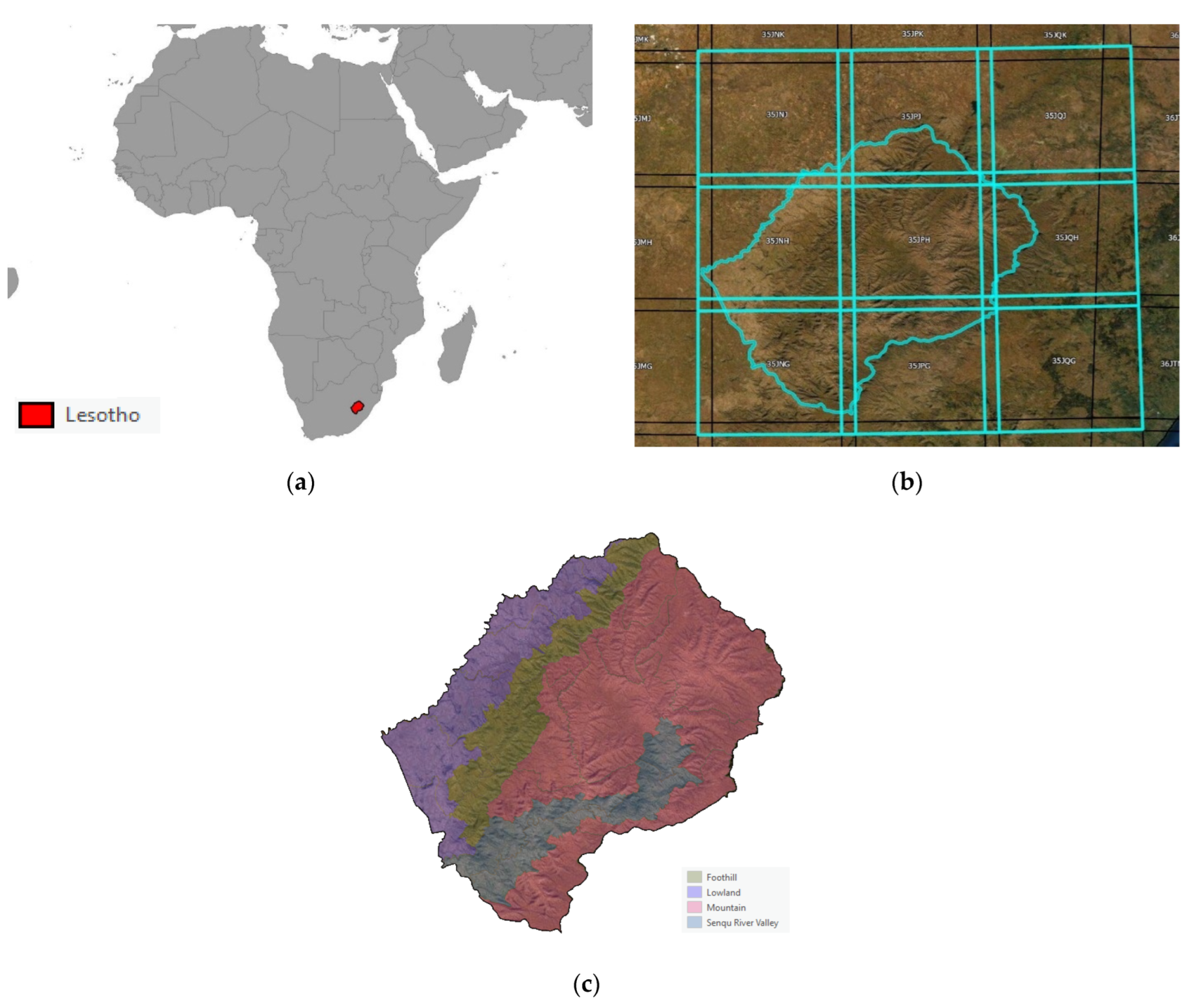
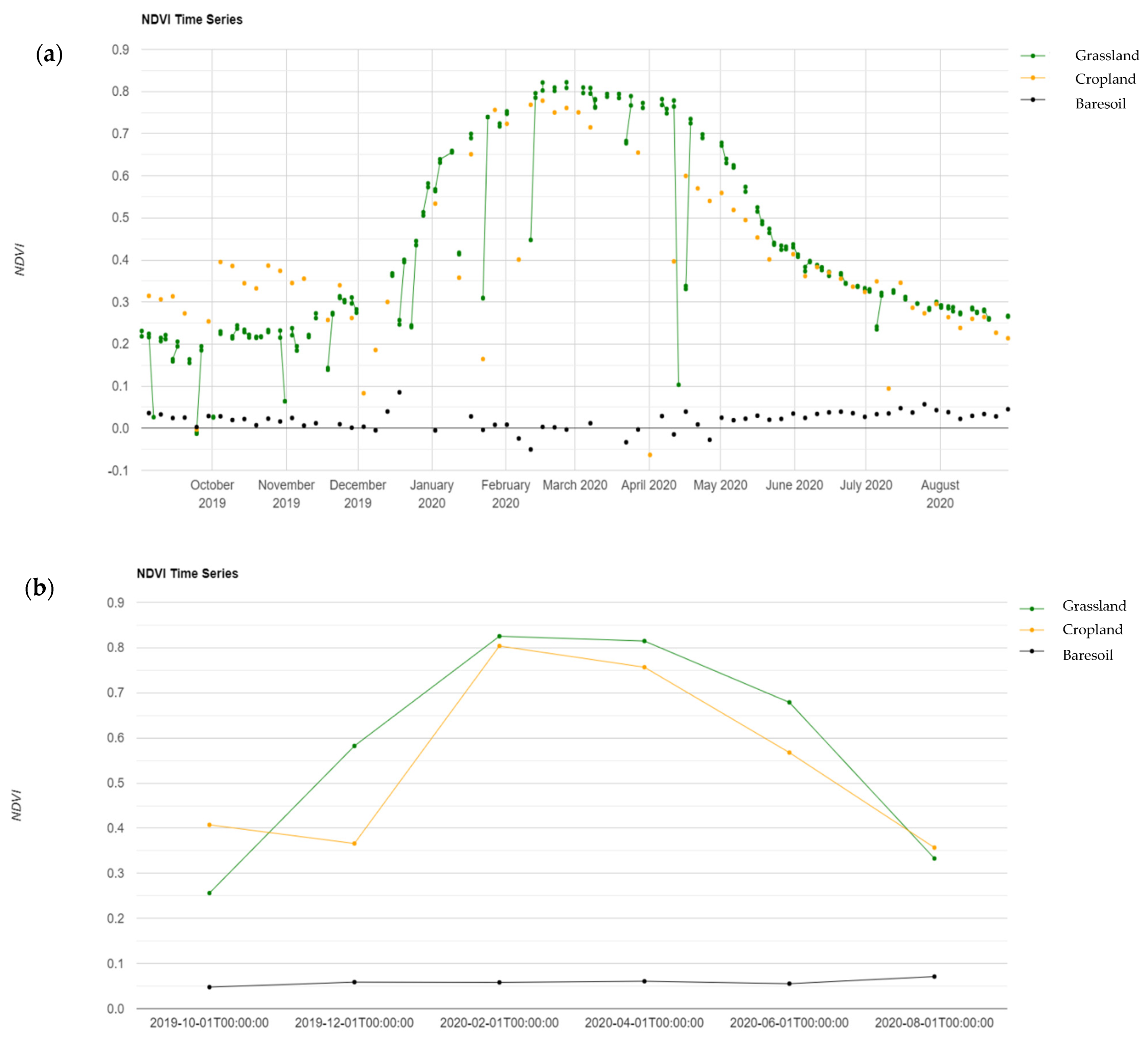
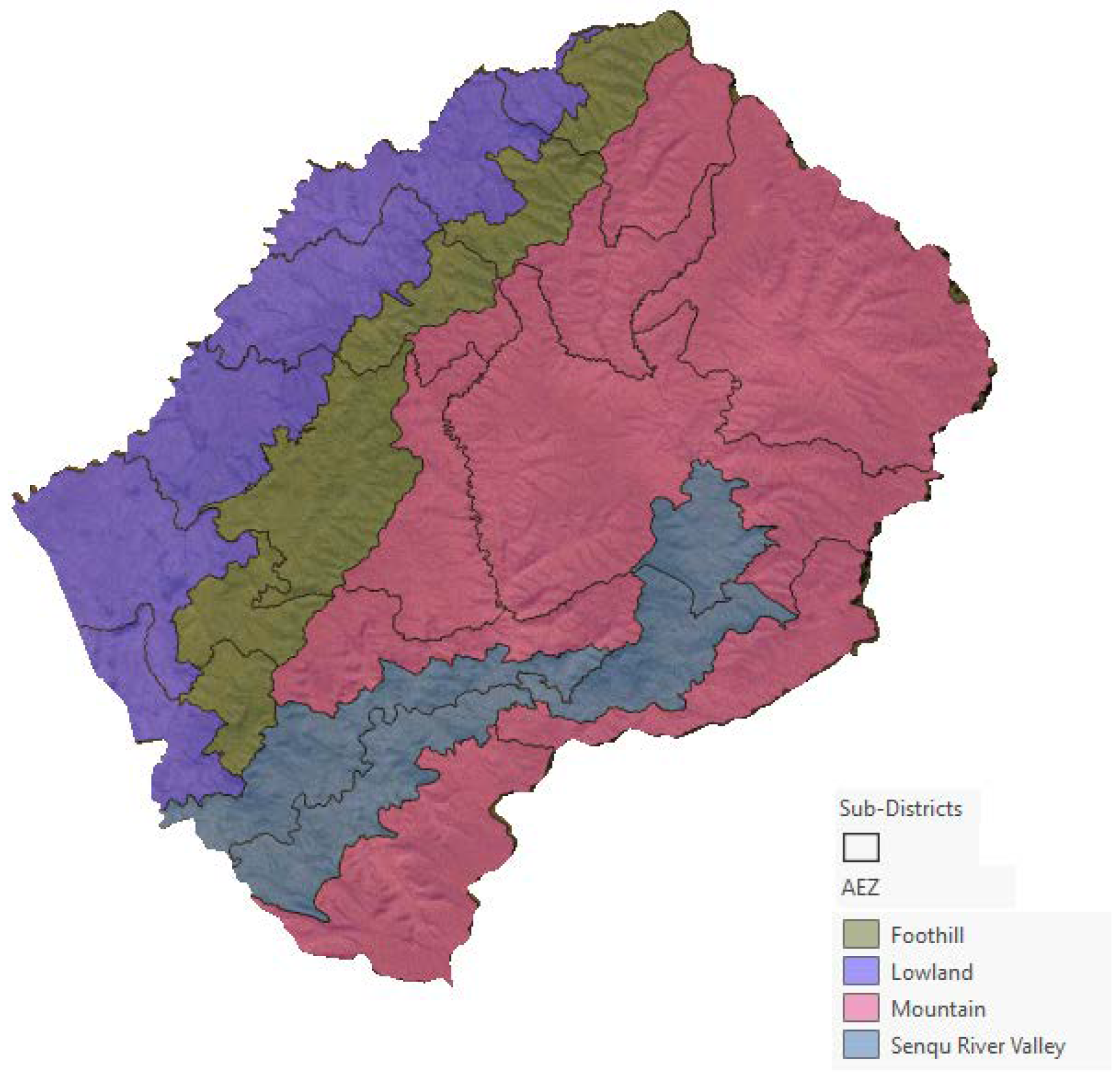
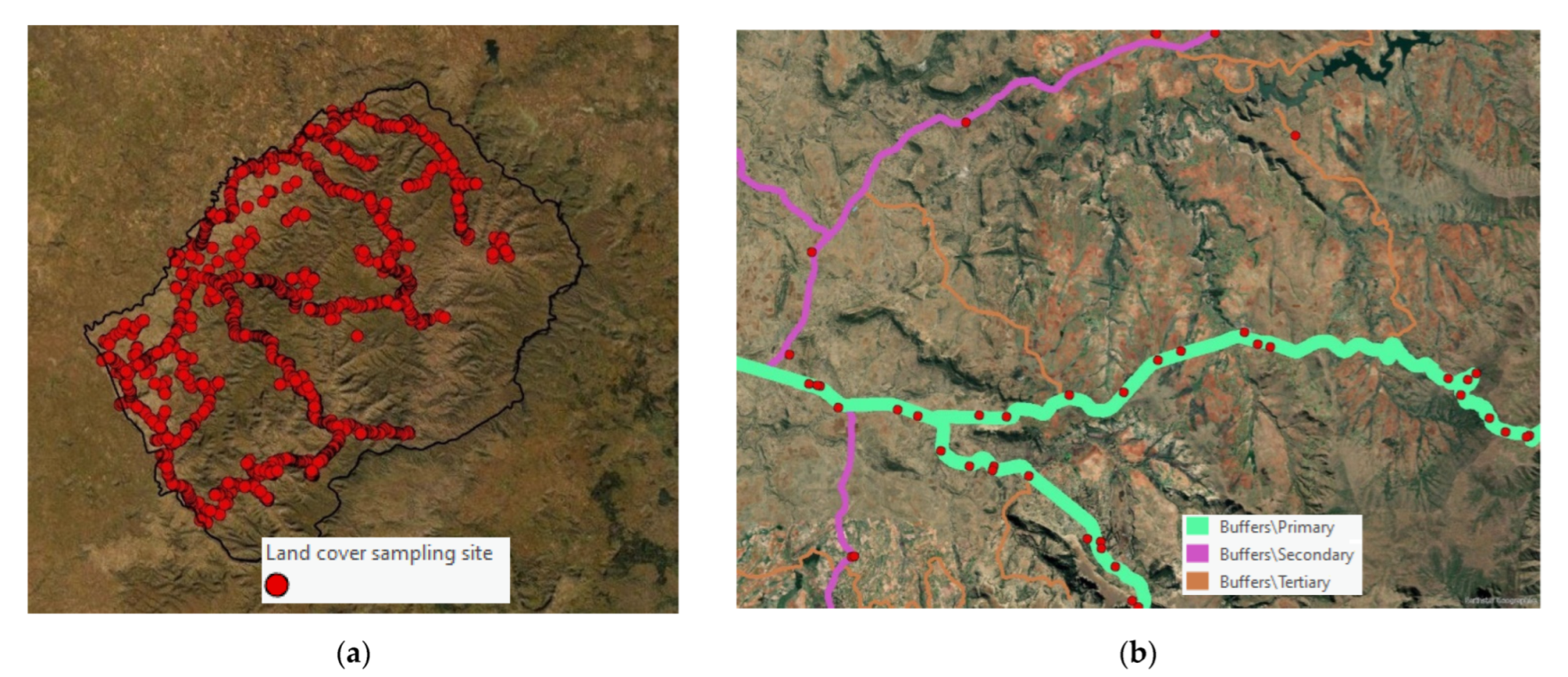
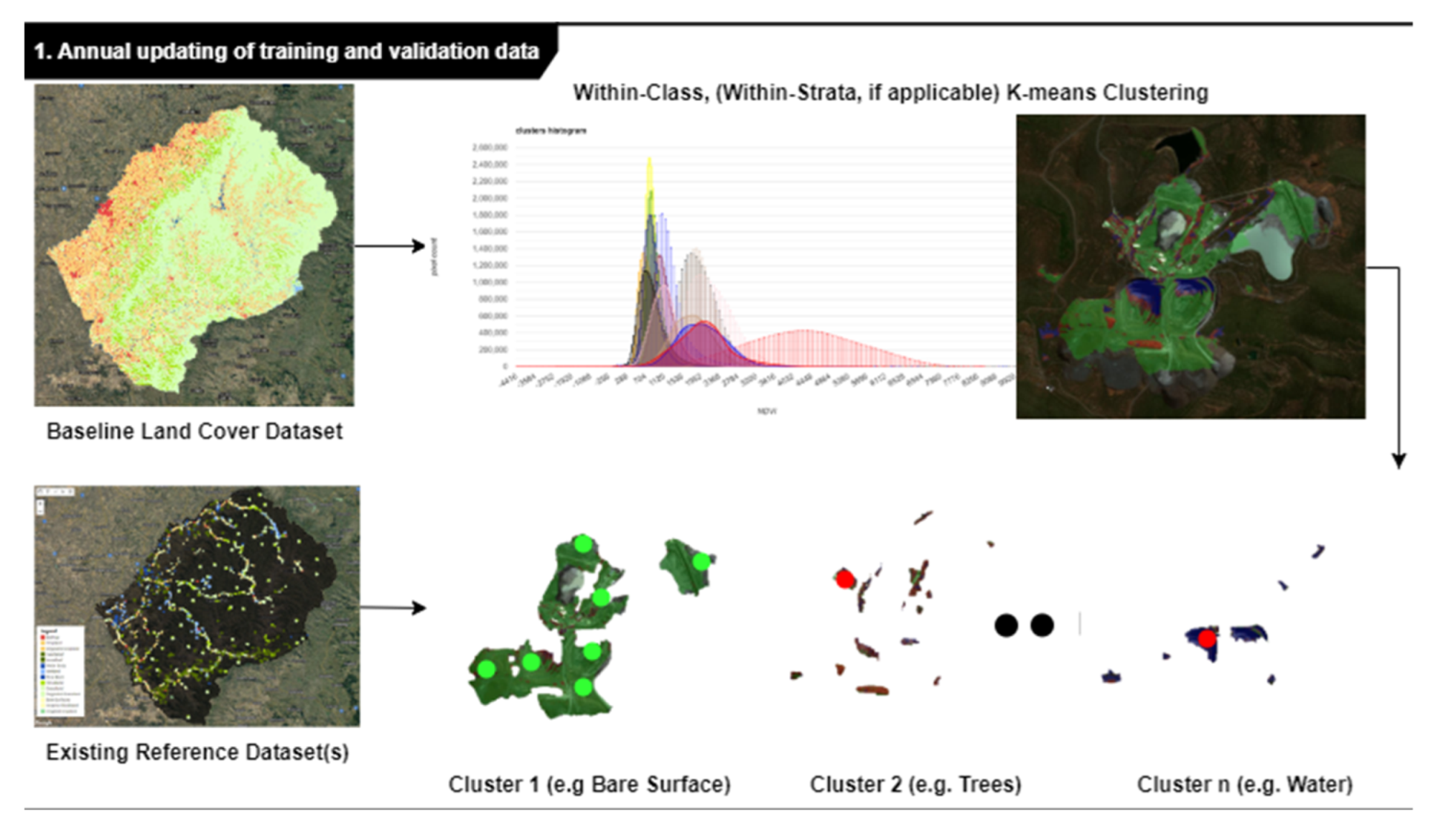
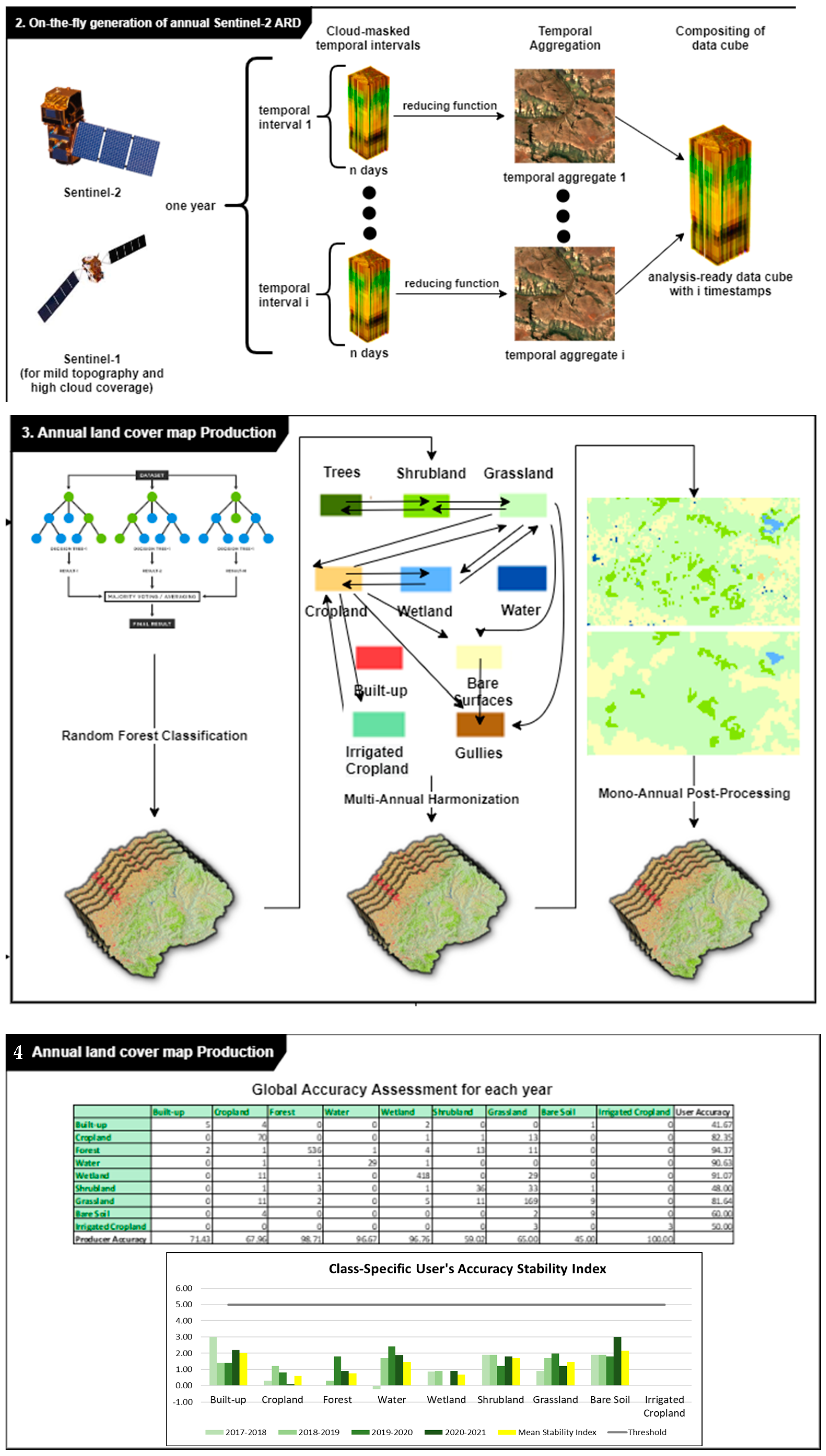
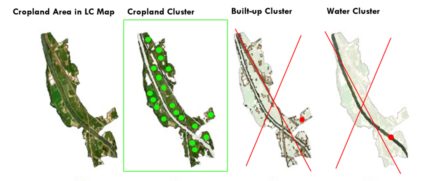
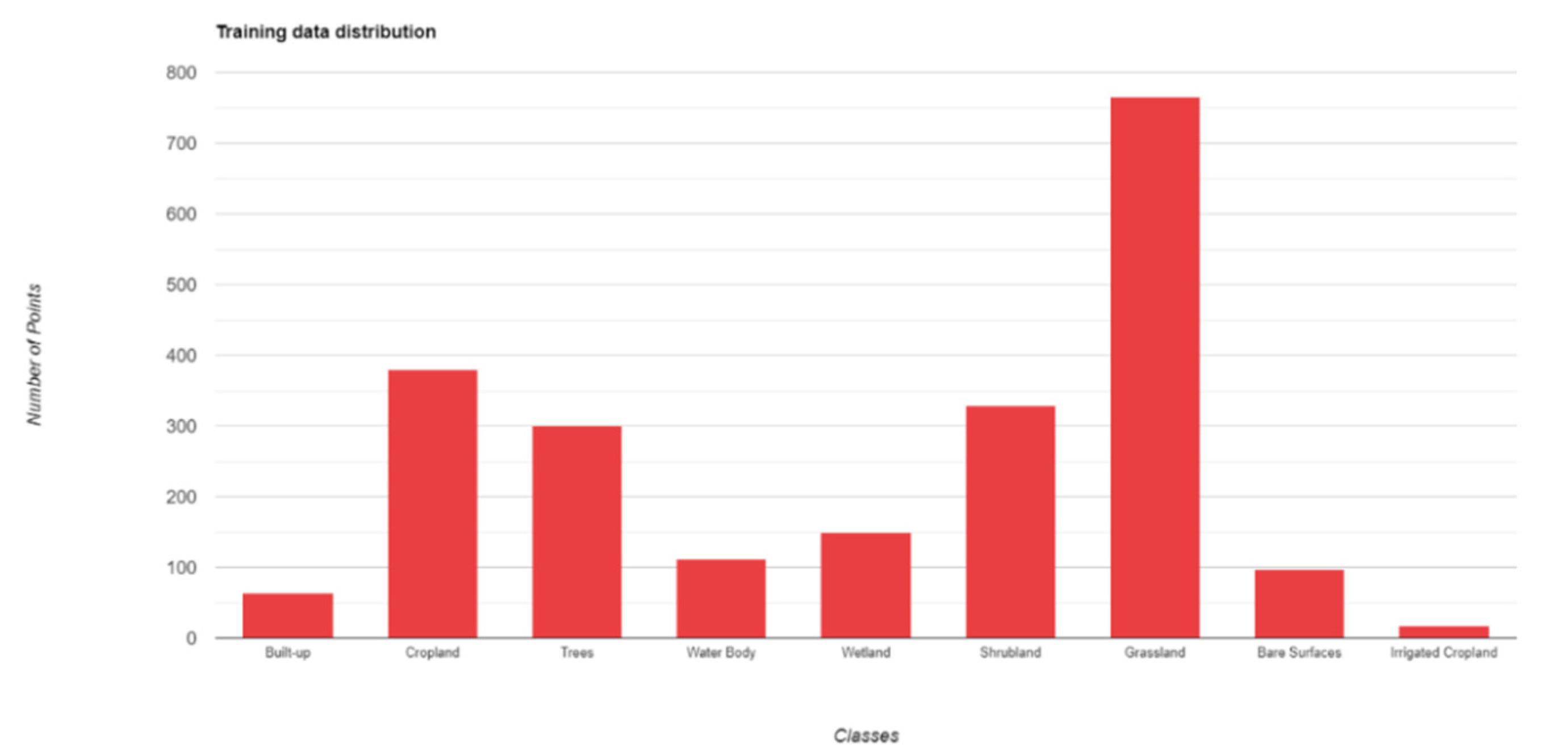
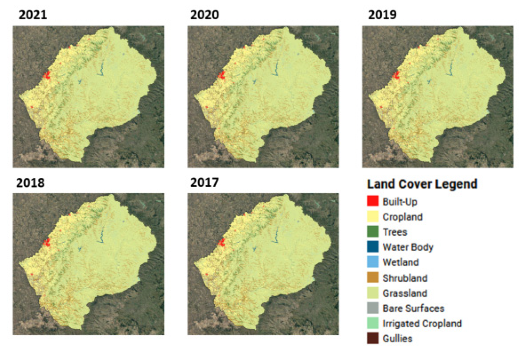
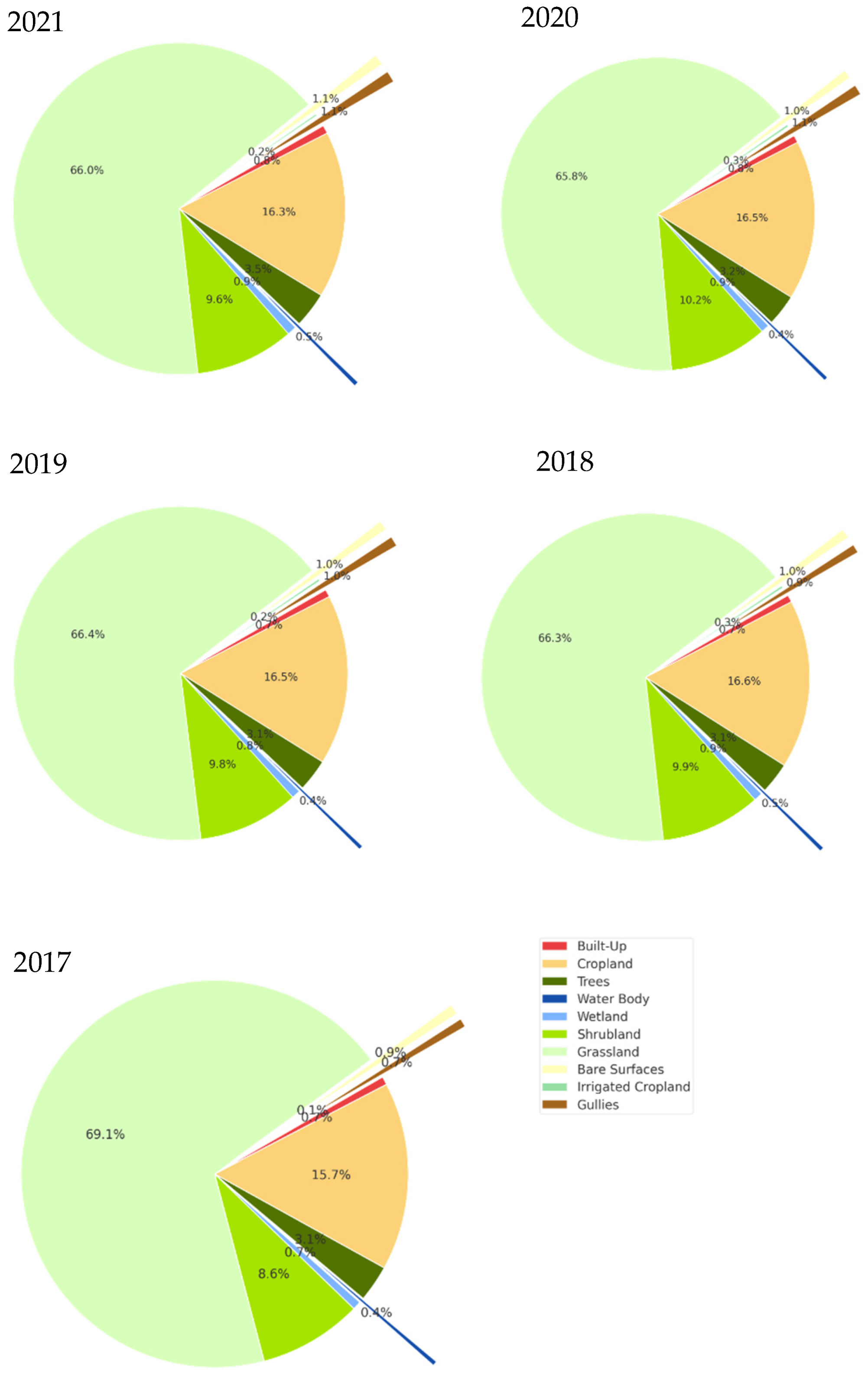
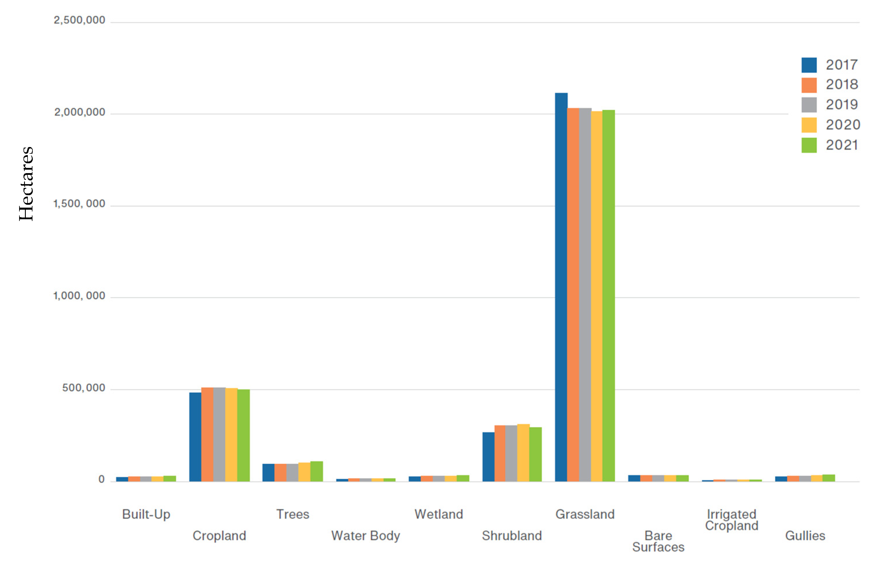
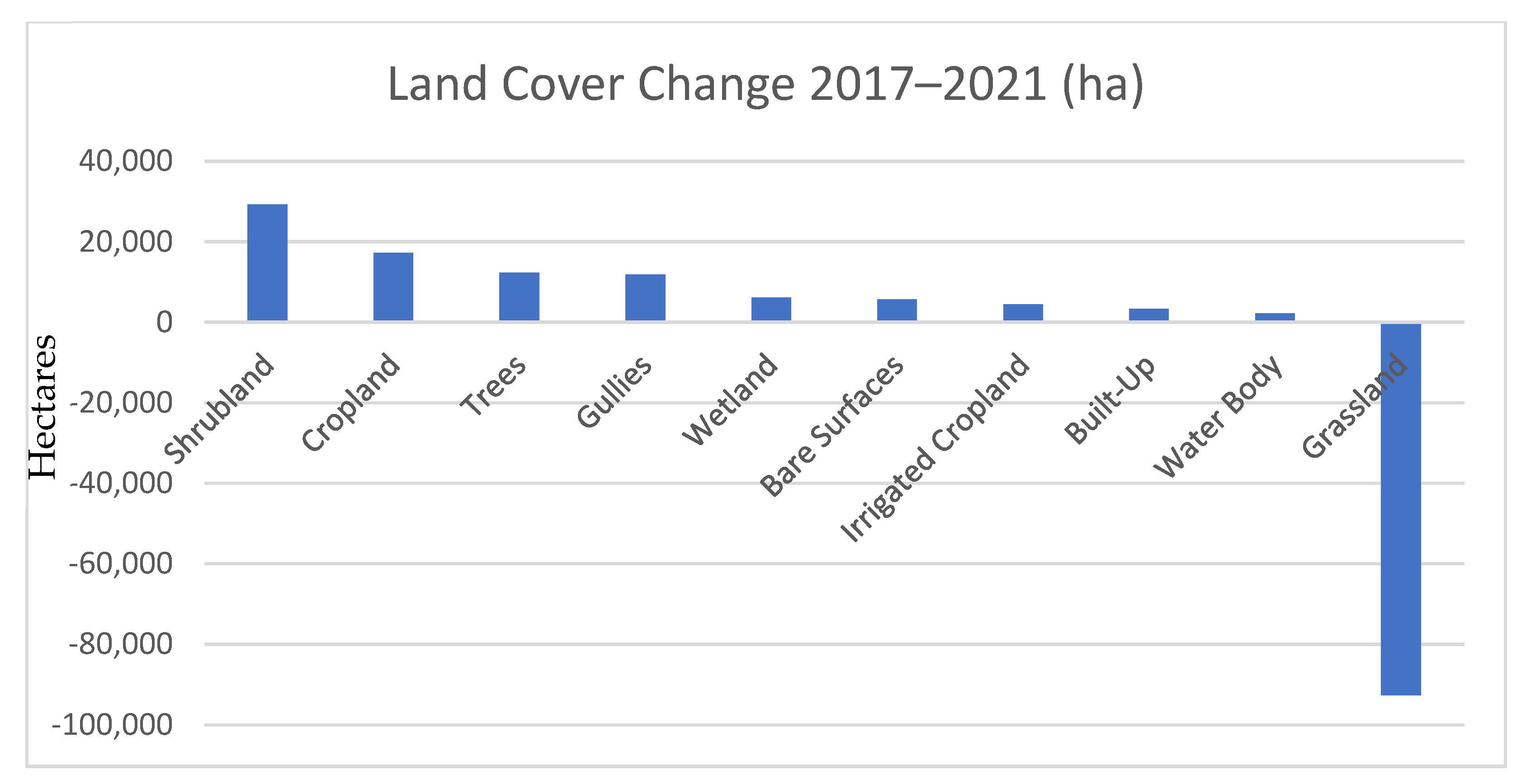
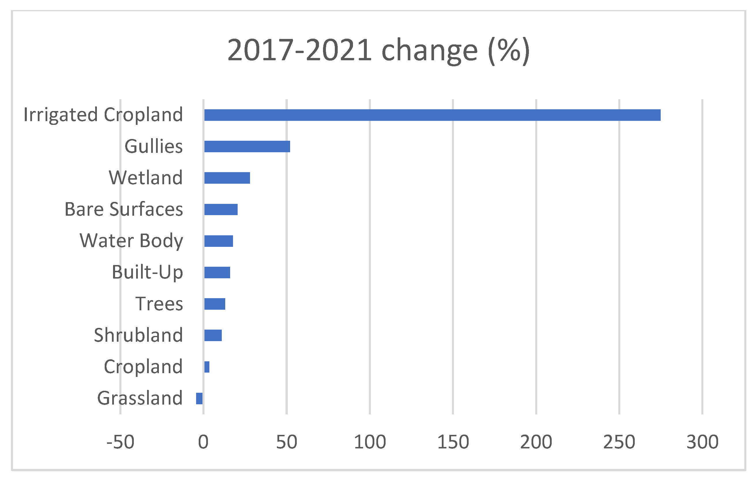
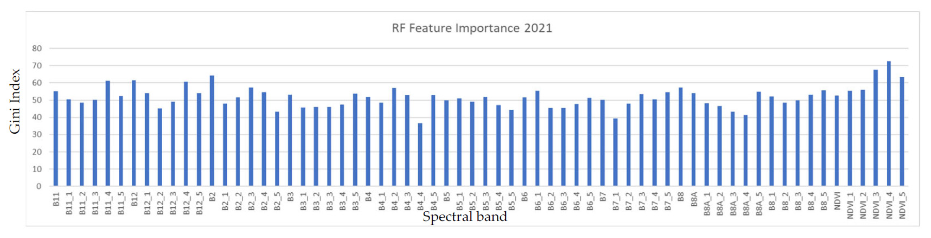
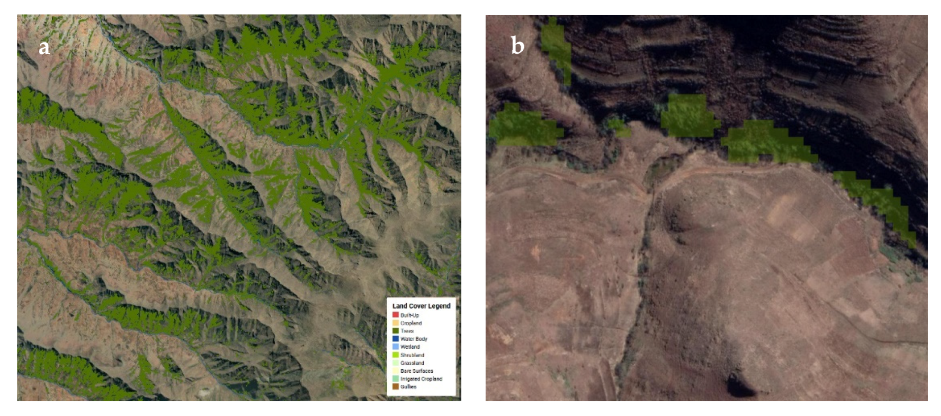
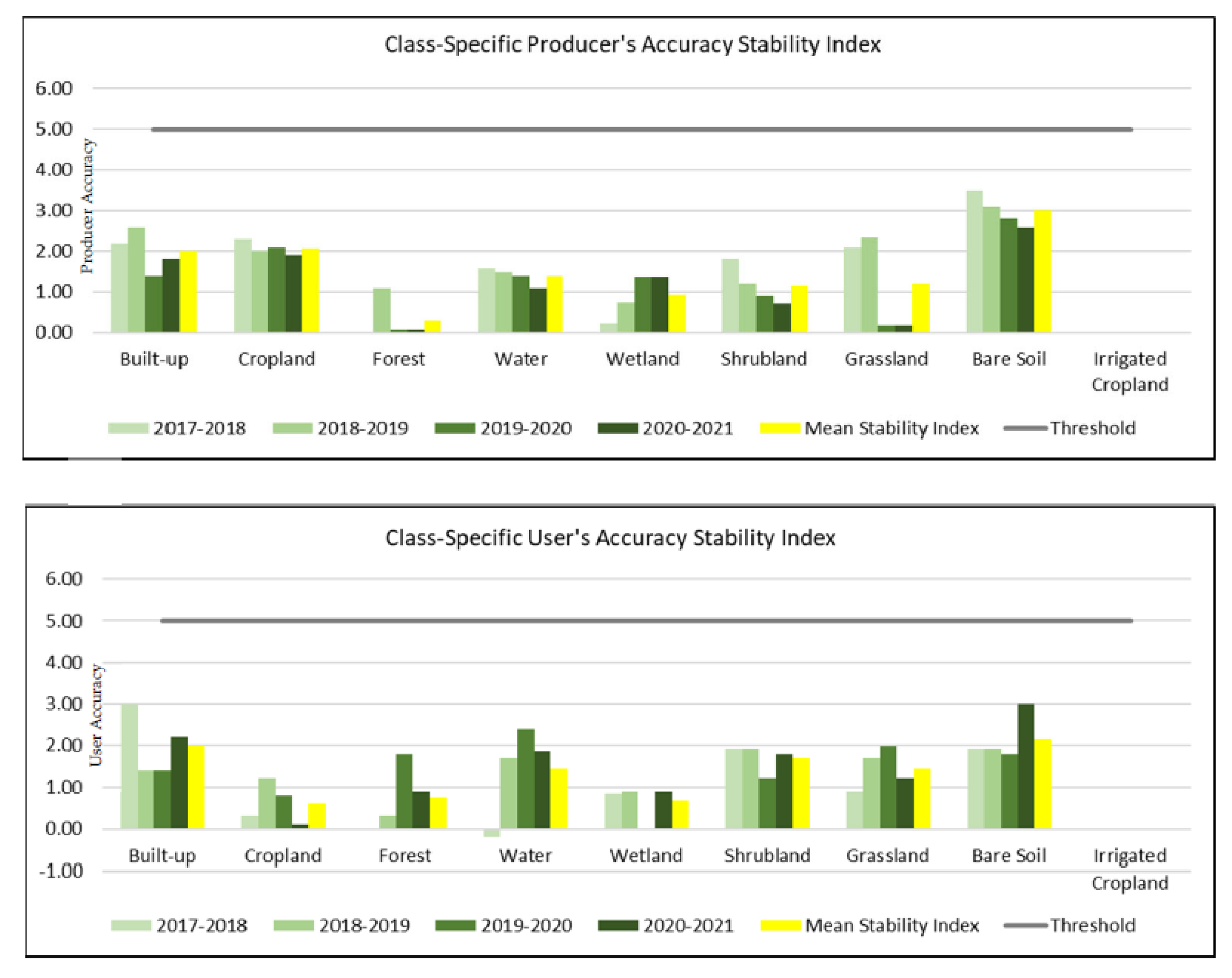
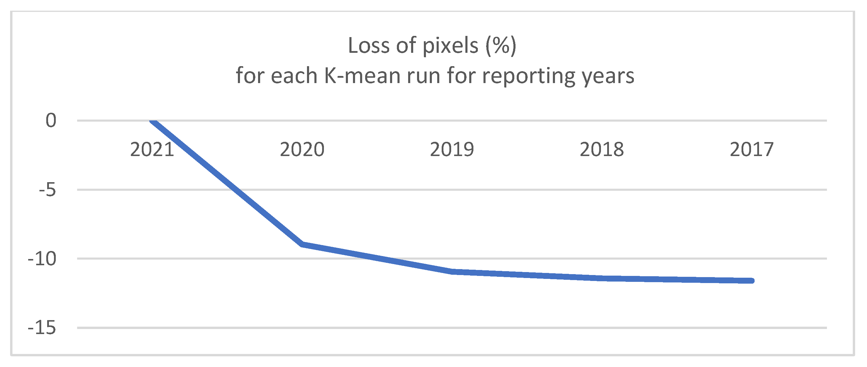
Table 1.
FAO LCL classes and their definitions.
| Land Cover Type | Code | Description |
|---|---|---|
| Urban | UA1 | Relatively larger urban built-up areas, commonly with presence of trees, occasionally with small, cultivated fields; scattered open areas observed in some areas. |
| Urban commercial/industrial | UA2 | Urban, commercial, and/or industrial built-up areas, occasionally outside main urban and rural built-up areas. |
| Rural settlements plain areas | RH1 | Rural houses in flat lying plain areas (slope up to 5 degrees) + small, cultivated herbaceous crops + closed herbaceous natural vegetation, often together with trees and/or shrubs employed for demarcation; scattered open areas observed in some areas. |
| Rural settlements sloping areas | RH2 | Rural houses in sloping and mountainous areas (slope greater than 5 degrees) + herbaceous natural vegetation, occasionally with small fields and sometimes with shrubs employed for demarcation, usually treeless. |
| Rainfed agriculture plain areas | HCP | Rainfed herbaceous crops cultivated in flat-lying plains (slope up to 10 degrees) with relatively larger-sized fields. |
| Rainfed agriculture sloping regions | HCSM | Rainfed herbaceous crops in sloping land and mountains (slope greater than 10 degrees) with terracing and/or contour ploughing, small- and medium-sized fields, sometimes with lines of shrubs demarcating fields. |
| HCER | Rainfed herbaceous crops with visible water sheet erosion, commonly with associated gully erosion. | |
| Irrigated agriculture | HCIR | Small size irrigated herbaceous crops near water courses |
| Rainfed agriculture–Rainfed orchards | HCT | Small rainfed herbaceous crops + regular rainfed orchard plantations (usually as rows of fruit trees separating elongated fields). |
| Trees, Needle-leaved (closed) | TNL1 | Closed evergreen needle-leaved trees, sometimes occurring as plantations. |
| Trees, Needle-leaved (open) | TNL2 | Open evergreen needle-leaved trees + herbaceous natural vegetation. |
| Trees, Broad-leaved (closed) | TBL1 | Closed deciduous broad-leaved trees, commonly along riverbeds, sometimes observed as plantations. |
| Trees, Broad-leaved (open) | TBL2 | Open deciduous broad-leaved trees + herbaceous natural vegetation. |
| Trees, Undiff. (closed) | TM1 | Closed undifferentiated trees, sometimes mixed broad-leaved and needle-leaved; occasionally with shrubs. |
| Trees, Undiff. (open) | TM2 | Open undifferentiated trees + herbaceous natural vegetation. |
| Trees (sparse) | TS | Sparse scattered trees + herbaceous natural vegetation (closed-open). |
| Large waterbody | WB1 | Large perennial freshwater lake or dam reservoir. |
| Small waterbody | WB2 | Small fresh water seasonal and/or perennial reservoir, pool, etc. sometimes associated with nearby wetland areas. |
| Wetland (perennial or seasonal) | WET | Natural perennial and/or seasonal fresh waterbody + perennial closed–open natural vegetation. |
| Riverbank | RB | Riverbank (soil/sand deposits) + perennial or periodic flowing freshwater (river), occasionally with loose scattered rocks, often with adjacent trees and shrubs. |
| Shrubland (closed) | SH1 | Closed Natural Shrubs (H = 0.5 to 1.5 m), commonly observed on river valley slopes, occasionally with scattered rocks and boulders. |
| Shrubland (open) | SH2 | Closed Natural Shrubs (H = 0.5 to 1.5 m), commonly observed on river valley slopes, occasionally with scattered rocks and boulders. |
| Grassland | GR | Grassland—relatively dense natural vegetation, occasionally with sparse shrubs. |
| Grassland–Degraded | GRD | Degraded grassland with low vegetative cover, occasionally bare with scattered rock outcrops; noticeably in sloping areas adjacent to main river valley. |
| Bare Rock | BR | Rock outcrops, commonly located at plateau edges. |
| Bare area | BA | Bare areas/undifferentiated areas not used for cultivation and usually devoid of grass or shrub cover, commonly associated with degraded land and erosion effects, sometimes within or adjacent to urban and rural areas. |
| Boulders and loose rocks | BLR | Areas with large, scattered boulders and/or unconsolidated loose rocks, commonly sloping and associated with rock outcrops, usually together with open–closed natural vegetation and/or shrubs and/or natural trees. |
| Gullies | GU | Gully erosion, commonly associated with riverbeds, occasionally with trees and/or tall shrubs. |
| Mines and Quarries | MQ | Major mines and quarries as well as temporary building material extraction and dumping sites. |
Table 2.
Spectrally heterogeneous classes present in the LCL 2015.
| LCS3 Type | LCS3 Code | Pixel Count (10 m) | Surface Area (km²) | % Total Area |
|---|---|---|---|---|
| Rural Settlements Plain Areas | RH1 | 7,826,416 | 782.6416 | 2.58% |
| Rural Settlements Sloping Areas | RH2 | 2,568,144 | 256.8144 | 0.85% |
| Rainfed Agriculture—Rainfed Orchards | HCT | 55,203 | 5.5203 | 0.02% |
| Trees, Needle-leaved (open) | TNL2 | 29,273 | 2.9273 | 0.01% |
| Trees, Broad-leaved (open) | TBL2 | 17,339 | 1.7339 | 0.01% |
| Trees, Undifferentiated (closed) | TM1 | 2,789,227 | 278.9227 | 0.92% |
| Trees, undifferentiated (open) | TM2 | 310,921 | 31.0921 | 0.10% |
| Trees (sparse) | TS | 286,691 | 28.6691 | 0.09% |
| Shrubland (open) | SH2 | 43,508,744 | 4350.8744 | 14.33% |
| Total | 57,391,958 | 5739.1958 | 18.91% |
Table 3.
Legend used for the new LCL.
| ID | Class |
|---|---|
| 1 | Built-up |
| 2 | Cropland Rainfed |
| 3 | Trees |
| 4 | Water bodies |
| 5 | Wetland |
| 6 | Shrubland |
| 7 | Grassland |
| 8 | Bare surfaces |
| 9 | Cropland Irrigated |
| 10 | Gullies |
Table 4.
Spectral bands from Sentinel-2 and criteria used for temporal aggregation.
| ID | Feature |
|---|---|
| 1 | Band 2 |
| 2 | Band 3 |
| 3 | Band 4 |
| 4 | Band 5 |
| 5 | Band 6 |
| 6 | Band 7 |
| 7 | Band 8 |
| 8 | Band 9 |
| 9 | Band 10 |
| 10 | Band 11 |
| 11 | Band 12 |
| 12 | NDVI |
Table 5.
Recommended number of samples from [31].
Table 5.
Recommended number of samples from [31].
| Land Cover Map Classes and Area of Test Site | Samples Per Class |
|---|---|
| <12 classes and <1 million acres (≈4000 km²) | 50 |
| >12 classes or >1 million acres (≈4000 km²) | 75–100 |
Table 6.
In situ data sample distribution across land cover classes for the 2021 dataset.
| Land Cover Class | Reference Set |
|---|---|
| Built-up | 88 |
| Cropland | 511 |
| Trees | 624 |
| Water | 168 |
| Wetland | 529 |
| Shrubland | 441 |
| Grassland | 1065 |
| Bare Surfaces | 132 |
| Irrigated Cropland | 23 |
| Gullies (derived through a separate process, as described in Section 3.4) | 1000 |
Table 7.
Table summarizing the differences between the 2015 and 2021 land cover methodologies.
| Methodological Component | LCDB 2015 | LCDB 2021 |
|---|---|---|
| Training Data Sourcing | Field Collected for Validation, Photointerpretation for labeling | Reuse and clean-up of existing land cover labels Targeted field survey to collect labels for land cover classes lacking labels |
| Image Resolution | 1.5/2 m (orthophotos, RapidEye) | 10 m (Sentinel-2) |
| Land Cover Nomenclature | 30 classes, including heterogeneous and fuzzy classes (e.g., open forest, degraded cropland, etc.) | 10 classes that are considered nonfuzzy and homogeneous (i.e., machine-learning-friendly) |
| Classification Method | Image Segmentation + Manual labeling of objects | Pixel-based Machine Learning Classifier (Random Forest) |
| Temporal analysis | Single time stamp | Time series analysis |
| Validation Approach | Not reported (manual production, but no statistics on quality of manual labeling) |
|
Table 8.
Reference land cover data gathered in the field (2021) and automatically generated (2017–2020), and the number of pixels contained in each dataset. Number of pixels decreases as the reference year becomes further apart from the baseline data (2021).
Table 8.
Reference land cover data gathered in the field (2021) and automatically generated (2017–2020), and the number of pixels contained in each dataset. Number of pixels decreases as the reference year becomes further apart from the baseline data (2021).
| Reference Data and Means of Collection | Reference Year | Number of Sampling Pixels |
|---|---|---|
| Field survey | Baseline 2021 | 3581 |
| Automatic K-Means | 2020 | 3260 |
| Automatic K-Means | 2019 | 3189 |
| Automatic K-Means | 2018 | 3172 |
| Automatic K-Means | 2017 | 3166 |
Table 9.
Training and Validation pixels per reference dataset generated from the reference dataset 2021.
Table 9.
Training and Validation pixels per reference dataset generated from the reference dataset 2021.
| Reference Year | Land Cover Class | Training Pixels | Validation Pixels |
|---|---|---|---|
| 2017 | Built-up | 73 | 13 |
| Cropland | 392 | 100 | |
| Trees | 300 | 279 | |
| Water | 107 | 27 | |
| Wetland | 150 | 324 | |
| Shrubland | 327 | 88 | |
| Grassland | 675 | 174 | |
| Bare Surface | 90 | 24 | |
| Irrigated Cropland | 12 | 11 | |
| Gullies | 800 | 200 | |
| Total | 2926 | 1240 | |
| 2018 | Built-up | 63 | 16 |
| Cropland | 381 | 93 | |
| Trees | 300 | 262 | |
| Water | 122 | 19 | |
| Wetland | 150 | 328 | |
| Shrubland | 327 | 87 | |
| Grassland | 712 | 175 | |
| Bare Surface | 87 | 27 | |
| Irrigated Cropland | 17 | 6 | |
| Gullies | 800 | 200 | |
| Total | 2959 | 1213 | |
| 2019 | Built-up | 74 | 11 |
| Cropland | 392 | 90 | |
| Trees | 300 | 258 | |
| Water | 108 | 21 | |
| Wetland | 150 | 311 | |
| Shrubland | 313 | 90 | |
| Grassland | 750 | 184 | |
| Bare Surface | 91 | 23 | |
| Irrigated Cropland | 20 | 3 | |
| Gullies | 800 | 200 | |
| Total | 2998 | 1191 | |
| 2020 | Built-up | 70 | 16 |
| Cropland | 385 | 77 | |
| Trees | 300 | 260 | |
| Water | 119 | 37 | |
| Wetland | 150 | 319 | |
| Shrubland | 318 | 93 | |
| Grassland | 797 | 181 | |
| Bare Surface | 92 | 23 | |
| Irrigated Cropland | 21 | 2 | |
| Gullies | 800 | 200 | |
| Total | 3052 | 1208 | |
| 2021 | Built-up | 64 | 12 |
| Cropland | 380 | 85 | |
| Trees | 300 | 268 | |
| Water | 111 | 32 | |
| Wetland | 150 | 309 | |
| Shrubland | 329 | 75 | |
| Grassland | 765 | 207 | |
| Bare Surface | 97 | 15 | |
| Irrigated Cropland | 17 | 6 | |
| Gullies | 800 | 200 | |
| Total | 3013 | 1209 |
Table 10.
Land cover statistics for the reference year, 2021.
| LC Class | Area ha | Area % |
|---|---|---|
| Built-Up | 24,541 | 0.8 |
| Cropland | 496,882 | 16.3 |
| Trees | 105,751 | 3.5 |
| Water Body | 14,801 | 0.5 |
| Wetland | 28,187 | 0.9 |
| Shrubland | 293,476 | 9.6 |
| Grassland | 2,018,449 | 66.0 |
| Bare Surfaces | 33,242 | 1.1 |
| Irrigated Cropland | 6087 | 0.2 |
| Gullies | 34,814 | 1.1 |
Table 11.
Accuracy results matrix for land cover 2021.
| Recall | Precision | F1 | |
|---|---|---|---|
| Built-up | 83.33 | 76.92 | 80.00 |
| Cropland | 74.47 | 90.91 | 81.87 |
| Trees | 98.7 | 96.93 | 97.81 |
| Water | 96.67 | 90.63 | 93.55 |
| Wetland | 97.21 | 91.47 | 94.25 |
| Shrubland | 68.97 | 47.62 | 56.34 |
| Grassland | 70.31 | 86.12 | 77.42 |
| Bare Soil | 65.22 | 83.33 | 73.17 |
| Irrigated Crops | 100.00 | 66.67 | 80.00 |
| Overall Accuracy | 89.86 | ||
| Kappa | 86.13 |
Table 12.
Unbiased Accuracy Assessment Summary Table.
| Class | Area (Hectares) | ±95% CI | User’s Accuracy (%) | Producer’s Accuracy (%) | Overall Accuracy (%) |
|---|---|---|---|---|---|
| Built-up | 23,855.70 | 1344.56 | 76.9 | 90.3 | 85.5 |
| Cropland | 564,535.47 | 33,694.95 | 90.9 | 80.0 | |
| Trees | 132,820.86 | 11,971.24 | 96.9 | 77.2 | |
| Water | 13,604.64 | 1564.28 | 90.6 | 98.6 | |
| Wetland | 85,244.03 | 14,745.40 | 91.5 | 40.2 | |
| Shrubland | 253,585.04 | 34,620.92 | 57.6 | 55.1 | |
| Grassland | 1,894,212.49 | 42,870.26 | 86.1 | 91.8 | |
| Bare soil | 52,439.78 | 17,020.61 | 83.3 | 52.8 | |
| Irrigated crops | 4058.00 | 1.07 | 66.7 | 100.0 |
Table 13.
Overall Accuracy of the annual national land cover maps.
| Year | 2021 |
|---|---|
| 2017 | 83.10% |
| 2018 | 83.65% |
| 2019 | 84.94% |
| 2020 | 85.69% |
| 2021 | 86.96% |
Publisher’s Note: MDPI stays neutral with regard to jurisdictional claims in published maps and institutional affiliations. |
© 2022 by the authors. Licensee MDPI, Basel, Switzerland. This article is an open access article distributed under the terms and conditions of the Creative Commons Attribution (CC BY) license (https://creativecommons.org/licenses/by/4.0/).
Share and Cite
MDPI and ACS Style
De Simone, L.; Ouellette, W.; Gennari, P. Operational Use of EO Data for National Land Cover Official Statistics in Lesotho. Remote Sens. 2022, 14, 3294. https://0-doi-org.brum.beds.ac.uk/10.3390/rs14143294
AMA Style
De Simone L, Ouellette W, Gennari P. Operational Use of EO Data for National Land Cover Official Statistics in Lesotho. Remote Sensing. 2022; 14(14):3294. https://0-doi-org.brum.beds.ac.uk/10.3390/rs14143294
Chicago/Turabian StyleDe Simone, Lorenzo, William Ouellette, and Pietro Gennari. 2022. "Operational Use of EO Data for National Land Cover Official Statistics in Lesotho" Remote Sensing 14, no. 14: 3294. https://0-doi-org.brum.beds.ac.uk/10.3390/rs14143294
Note that from the first issue of 2016, this journal uses article numbers instead of page numbers. See further details here.