A Multi-Rotor Drone Micro-Motion Parameter Estimation Method Based on CVMD and SVD

Abstract

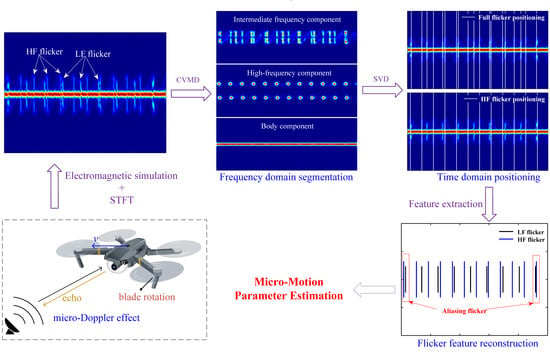
It is of great significance to detect drones in airspace due to the substantial increase and regrettable misuse in the consumer market. In this paper, we establish a micro-motion theoretical model of a drone and analyze the micro-Doppler signature of rotor targets and the flicker mechanisms of the multi-rotor targets. Hence, for the target recognition problem of multi-rotor drones, a multi-rotor target micro-Doppler parameter estimation method is proposed. Firstly, a signal frequency domain segmentation method is proposed based on the complex variational mode decomposition (CVMD) to separate the high-frequency part of the high-frequency flicker in the frequency domain. Secondly, for the signal after frequency domain segmentation, a flicker time domain position method based on singular value decomposition (SVD) is proposed. Finally, by integrating CVMD frequency domain segmentation and SVD time domain positioning, the reconstruction of multi-rotor target scintillation at different speeds is realized, and the micro-motion parameters of rotor blades are successfully estimated. The simulation results show that the method has high accuracy in estimating the micro-motion parameters of a multi-rotor, which makes up for the shortage of the traditional method in estimating the micro-motion parameters of the multi-rotor target.

1. Introduction

With the development of drone technology, commercial drones have gained huge popularity in recent times, due to their ease of operation, robust performances, and low costs. Drones have been widely used in agricultural operations, video shooting, logistic transport, environmental monitoring, and rescue assistance [1]. Along with their advantages, the usability of drones also brings significant potential safety hazards, especially “black flight” and illegal activity. Small drones usually have the characteristics of low-altitude flights, small radar cross-sections (RCSs), and slow speeds (“low, small, slow”), and have very similar radar characteristics to some large birds and other jamming targets. It is difficult to distinguish these targets using traditional radar detection methods [2].

Research on the micro-Doppler effect provides a practical technical approach for identifying drones. The micro-Doppler theory was first proposed by V. C. Chen from the US Naval Laboratory [3]; it is used to represent the Doppler effect caused by the micro-motion of the various components within a target. Nowadays, micro-Doppler signatures are widely used in radar target recognition and micro-motion parameter estimation [4,5,6]. The micro-motion of the drone is generated by the propeller blade rotation, and the bird is due to the flapping of the wings. These two micro-motion forms are entirely different, so there is apparent diversity in their micro-Doppler characteristics [7]. The study of micro-Doppler signatures is hence of great importance in this context [8].

The rotation of the rotor target will produce periodic modulation of the radar signal. When the rotor is at its maximum RCS position, the echo signal peaks, causing periodic flickering of the echo signal received by the radar. The flickering signal is displayed in a time–frequency spectrum as a series of equidistant flicker bands with a specific frequency domain width. This flicker band is a typical micro-Doppler signature of rotor targets. The micro-motion parameters can be estimated by analyzing the flickering time, flickering interval, flickering width, et al. At this time, it is essential to construct a reasonable and reliable mathematical model to represent the mathematical relationships visually [9,10,11]. The most classic echo model of the rotor target is the scattering point integral model proposed by V. C. Chen [12]. This echo model does not involve electromagnetic scattering properties, and the target characteristics are inherent in the echo amplitude and phase [13]. In addition, some researchers use electromagnetic simulations to obtain echo data to obtain more reliable simulation data [14]. Arne Schröder et al. [15,16] used the electromagnetic simulation software HFSS to conduct a detailed study on the electromagnetic characteristics of the multi-rotor drone. The results show that the multi-rotor drone body component only increases the contribution of the spectral zero-frequency component of the echo signal. Furthermore, the multiple rotors result in the superposition of flickering with different initial phases.

After investigation, we classified the micro-motion parameter estimation method of the rotor target into two types: parametric and non-parametric. The parametric method constructs the mathematical expression of the target’s micro-Doppler characteristics through prior knowledge of the target’s micro-motion form. It obtains the target’s micro-Doppler parameters through an optimal parametric search. Related methods in the literature include orthogonal matching pursuit (OMP) [17], phase compensation [18], the optimal estimation of the demodulation operator [19], and the Hough transform [20]. This class of algorithms relies on the optimal model’s accuracy. It is easy to fall into the optimal local solution, and high-dimensional parameters lead to excessive calculation amounts. The non-parametric method mainly obtains the micro-Doppler parameter information directly by analyzing the target echo signal and time–frequency spectrum. The most basic non-parametric method involves directly labeling the time–frequency spectrum and the Doppler frequency spectrum [21]. This method has a significant error, is easily affected by subjective factors, and is not suitable for processing large amounts of data. Other methods, such as the sum of cadence velocity diagram (SCVD) [22] and chopping frequency analysis [23], can be applied to estimate the rotor rotation frequency. The SVD left singular vector analysis and the Doppler frequency spectrum bandwidth analysis can be rented for the Doppler bandwidth [24]. However, these methods depend on the target’s stable rotational speed and long-term echo accumulation. In addition, the cepstrum [25] and auto-correlation cepstrum [26] are used to estimate the rotor velocity. For the target with multiple rotors, its micro-Doppler signature has more flicker. Moreover, the corresponding flicker will show different frequency domain bandwidths when the blades rotate at different speeds. These phenomena will significantly increase the difficulty of the micro-motion parameter estimation. It is difficult to estimate the micro-motion parameters of the multi-rotor target using traditional non-parametric parameter estimation methods.

Regarding the problem of achieving multi-rotor drone parameter estimation, this paper proposes a parameter estimation method based on CVMD and SVD according to the flicker feature of the multi-rotor. Firstly, the paper constructs the theoretical echo model of the multi-rotor drone and analyzes and verifies the mechanism and characteristics of the flicker caused by the rotation of the multi-rotor. Secondly, CVMD is used for the frequency domain segmentation of the blade flicker, which can separate the high-frequency part of the high-frequency flicker in the frequency domain according to the frequency domain characteristics of the signal. Then, by feature extraction of the right singular vector obtained by SVD, the accurate estimation of the scintillation time domain position is realized. Finally, the proposed method is verified by theoretical simulation and electromagnetic simulation data. The experimental results show that the proposed method can accurately estimate the multi-rotor blade parameters, including the flicker period, maximum micro-Doppler frequency, and blade length.

The structure of this paper is as follows. In Section 2, the flickering mechanism of the multi-rotor target is analyzed through the micro-motion model of the rotor target. Section 3 presents a method for estimating micro-motion parameters of multi-rotor targets. Section 4 analyzes and tests the proposed algorithm. Section 5 analyzes and discusses the algorithm’s performance. The last, Section 6 concludes the paper and provides an outlook for future research.

2. Analysis of Flickering Mechanism of Multi-Rotor Drone

In this section, the relationship between the flicker mechanism of the multi-rotor drone and the state of the rotor blades is analyzed in detail. The relationship between the motion dynamics and radar echo signal induced by the rotating blades of the drone is presented firstly. After that, the flicker mechanism of the multi-rotor micro-Doppler signature is analyzed in detail using the theoretical simulation results of the echo model. Moreover, the electromagnetic simulation is used to verify the correctness of the theoretical simulation results.

2.1. Echo Mathematical Model of a Flying Drone

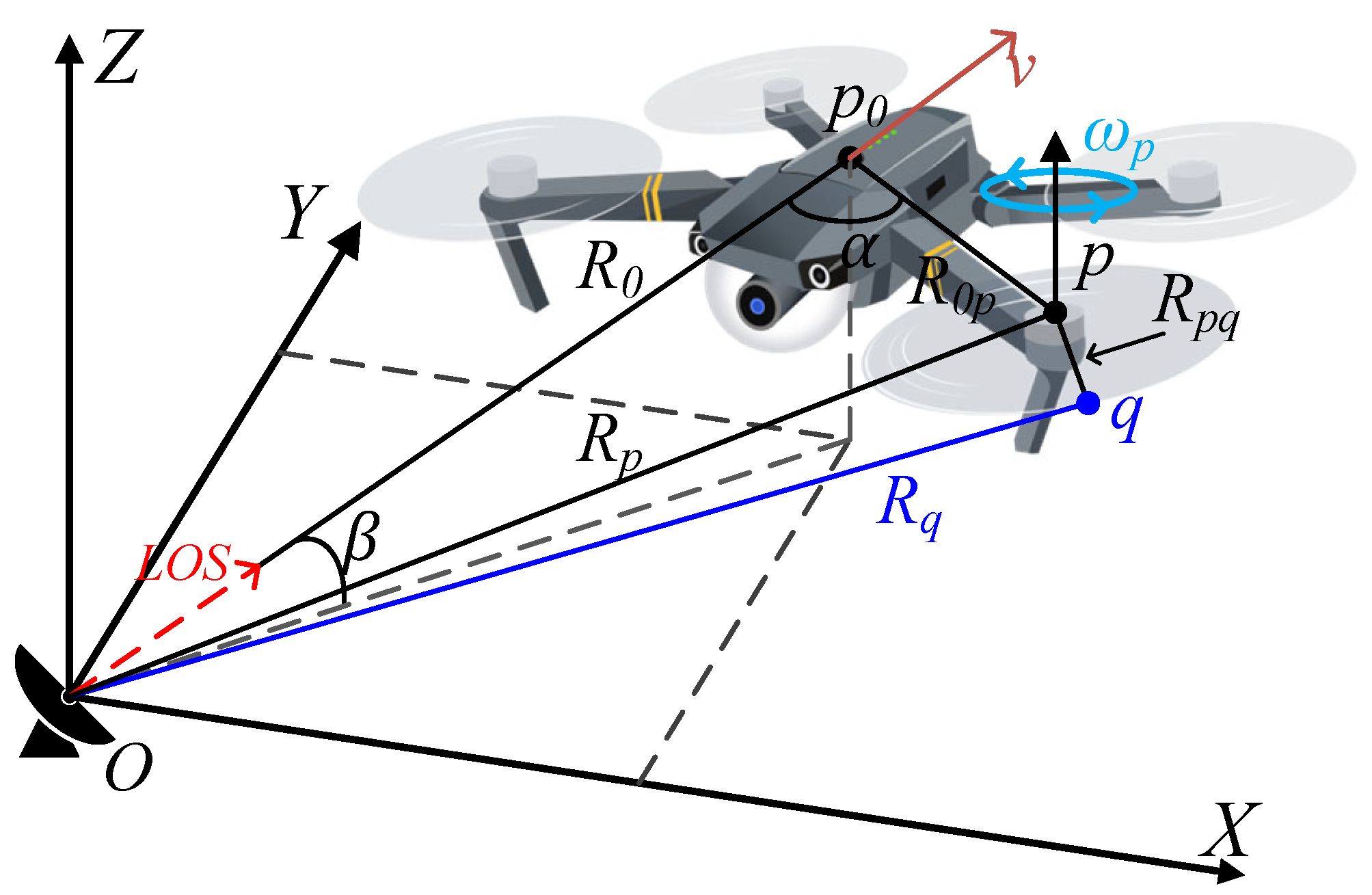
The dynamic geometric relationship between the rotor drone with its rotating blades and the radar is shown in Figure 1. The radar is located at the origin of the $XYZ$ coordinate system, $R_0$ is the distance from the radar center along the radar line of sight (LOS) to the drone center $p_0$ at the initial moment, and $\beta$ is the angle between $R_0$ and the $XOY$ plane. The distance between the rotor center p and the drone center $p_0$ is $R_{0p}$, and the angle between $R_0$ and $R_p$ is $\alpha$. It is assumed that the drone’s main body and micro-motion of its blades can be modeled using the constant radial velocity v and constant angular velocity ${\omega }_p$. Referring to [23], the echo signal received from the entire drone can be expressed in the time domain as

$$s\left(t\right)=\overline{A}·s_T\left(t\right)+\overline{B}·s_T\left(t\right)·s_M\left(t\right),$$

(1)

where

$$\overline{A}=\sum _{k=1}^K{A}_{k}exp\left\{-j\frac{4\pi }{\lambda }\left(R_0-R_{k}cos\alpha \right)\right\},$$

(2)

$${\overline{B}}_{pq}=B_{pq}exp\left\{-j\frac{4\pi }{\lambda }\left(R_0-R_{p}cos\alpha \right)\right\},$$

(3)

$$s_T\left(t\right)=exp\left\{-j2\pi \left(f_0+\frac{2v}{\lambda }\right)t\right\},$$

(4)

$$s_M\left(t\right)=\sum _{p=1}^P\sum _{q=1}^Q{\overline{B}}_{pq}exp\left\{-j\frac{4\pi }{\lambda }{r}_{pq}cos(R_k+{\omega }_{p}t)cos\beta \right\},$$

(5)

in which $f_0$ is the radar carrier frequency and $\lambda$ is the wavelength. K is the number of body scatters, $A_k$ is the scattering intensity of the kth scatterer, and $R_p$ is the distances between scatters k, p, and $p_0$. ${\alpha }_k$ is the angle between $O{p}_0$ and $p_{0}k$. P is the number of drone rotor blades, Q is the number of scattering points on the blade, $B_{pq}$ is the scattering intensity of the scattering point q on the rotor p, and $R_{pq}$ is the distance between the blade scattering point q on the rotor p and the rotor axis of p. ${\phi }_{0pq}$ is the initial phase of the scattering point q on the rotor p, ${\phi }_{0p}$ is the initial phase of the rotor p, N is the number of rotor blades, and ${\phi }_{0pq}$ satisfies

$${\phi }_{0pq}={\phi }_{0p}+2\pi (n-1)/N,n=1,\cdots ,N-1.$$

(6)

The frequency domain analysis can be obtained by taking the Fourier transform (FT) of the time domain echo:

$$S\left(f\right)=A·\delta (f+f_0+\frac{2v}{\lambda })+\delta (f+f_0+\frac{2v}{\lambda })*S_M\left(f\right),$$

(7)

where * is the convolution operation, and $\delta (·)$ is the Dirac function. Expanding $s_M\left(t\right)$ with a Fourier series and referring to the Bessel function of the first kind, Equation (7) can be approximately expressed as

$$S\left(f\right)\approx A·\delta (f+\frac{2v}{\lambda })+\sum _{p=1}^P\sum _{q=1}^Q\sum _{-\infty }^{\infty }{\overline{B}}_{pq}{C}_{pq}\left(Nm\right)\delta (f+\frac{2v}{\lambda }-\frac{N{\omega }_p}{2\pi }m),$$

(8)

where

$$C_{pq}\left(m\right)=J_m(\frac{4\pi }{\lambda }{r}_{pq}cos\beta )exp\left\{jm({\phi }_{0pq}-\frac{\pi }{2})\right\},$$

(9)

where $J_m(·)$ is the mth-order Bessel function of the first kind. Referring to Equation (9), it can be known that the Doppler frequency range of the echo signal is

$$\left[f_{dmin},f_{dmax}\right]=\frac{2}{\lambda }\left[-v-R_{pq}{\omega }_{p}cos\beta ,-v+R_{pq}{\omega }_{p}cos\beta \right].$$

(10)

2.2. Theoretical Simulation Analysis of Flicker Mechanism and Electromagnetic Simulation Verification

In this paper, the simulation of the quad-rotor echo is based on the continuous wave (CW) radar with a carrier frequency of 10 GHz and a pulse repetition frequency of 20 kHz, and the blade scatters are regarded as a scattering line segment composed of a series of scattering points. Assume that the radar and the drone are on the same horizontal altitude; that is, the LOS angle $\beta$ is $0^{\circ }$, the initial distance $R_0$ is 50 m, and the length of the blade is $0.1\sqrt{2}$ m. In addition, to analyze the flicker features, it is assumed that the Doppler frequency shift caused by the translation motion of the drone is compensated. The simulation includes two typical motion states, hovering and horizontal uniform motion. In other drone states, considering the short observation time, the drone’s blades can be approximately regarded as rotating at a uniform speed. At this time, the state of the drone can be approximately regarded as one of these two basic states. The setting parameters of the drone are shown in

Table 1. Drone simulation parameters in different states.

Type	Attitude Angle $\mathit{\theta }{(}^{\circ })$	Rotors Rotating Velocity ${\mathit{\omega }}_{\mathit{p}}/2\mathit{\pi }$ (rad/s)	Blade Phase ${\mathit{\phi }}_0{(}^{\circ })$
1	0	50	45
2	0	[50, −50, −50, 50]	[45, 45, 45, 45]
3	0	[50, −50, −50, 50]	[45, 135, 135, 45]
4	0	[50, −50, −50, 50]	[0, 45, 45, 0]
5	0	[50, −50, −50, 50]	[45, 60, 90, −25]
6	30	[45, −61, −45, 61]	[45, 135, 135, 45]
7	0	[45, −61, −45, 61]	[0, 25, 127, 100]
8	60	[60, −80, −60, 80]	[45, 135, 135, 45]

.

The parameter settings in Table 1 are based on the consideration of the essential force balance of the drone. (1) The sum of rotational inertia generated by the rotation of all the rotors of the drone is zero. The general control model sets the steering of the angular rotors to be the same and the steering of the adjacent rotors to be opposite. (2) The lift generated by the drone under various attitudes can balance its gravity. Assume that the quadratic sum of the rotation speed required for the hovering state of the drone is $\mathrm{\Omega }$. Then the blade rotating velocity satisfies the following relationship:

$$\left\{\begin{array}{c}{\omega }_1+{\omega }_2+{\omega }_3+{\omega }_4=0\\ \left({\omega }_1^2+{\omega }_2^2+{\omega }_3^2+{\omega }_4^2\right)cos\theta =\mathrm{\Omega }\end{array}\right.$$

(11)

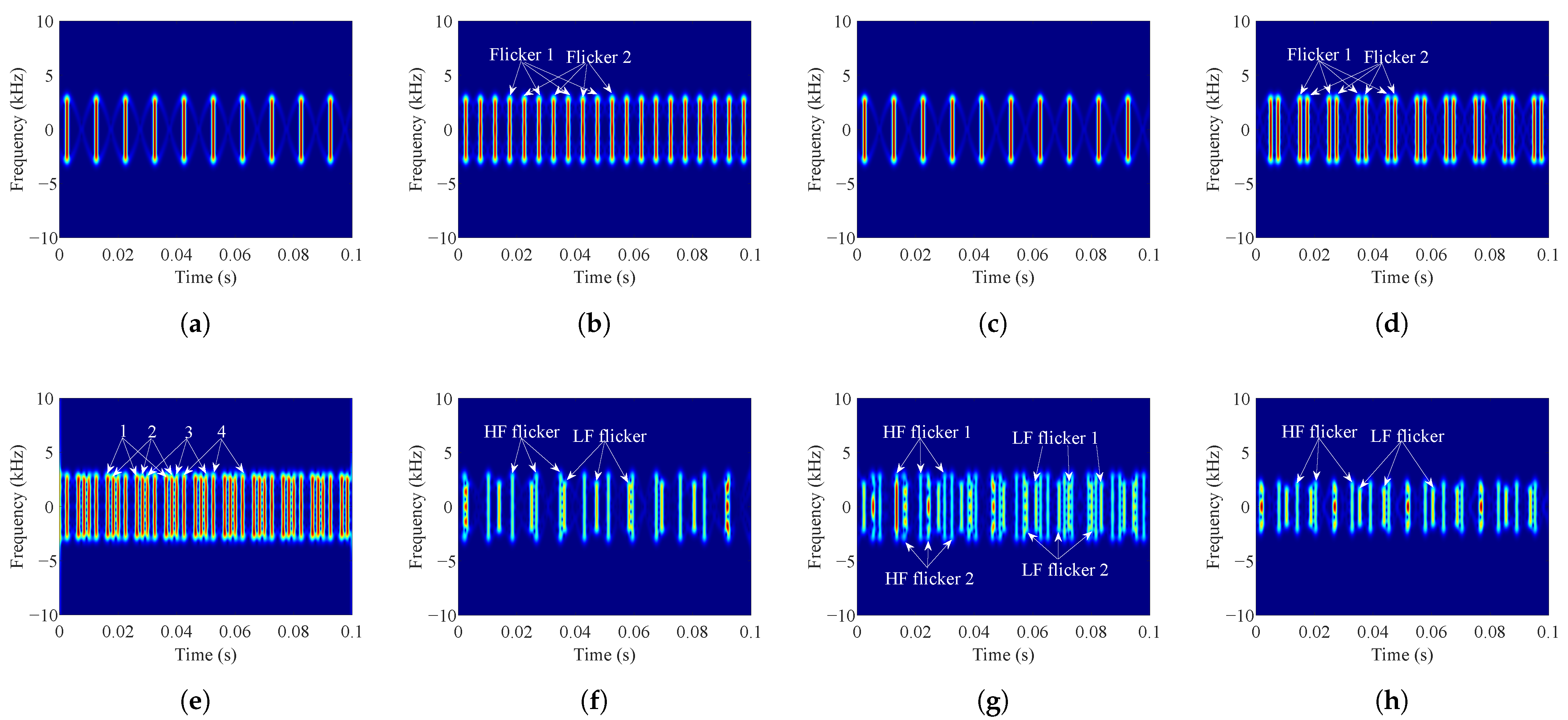
The time–frequency spectrum obtained by the short-time Fourier transform (STFT) of the quad-rotor blades echo simulation results in Table 1 is shown in Figure 2. The frequency spectrum simulation of a single-rotor blade is mainly used for the comparative experiment of multi-rotor simulation, which consists of a group of periodic flickers (shown in Figure 2a). Comparing Figure 2a–d, it can be seen that the quad-rotor echo frequency spectrum can be seen as composed of two groups of flickers. The diagonal rotor-corresponding flickers are completely coincident and caused by the same rotating velocity and initial phase. To analyze the relationship between the relative position changes of the two groups and the initial phase of the blades, the two groups of the rotor blade’s initial phase and the positions ${\phi }_{01}$, ${\phi }_{02}$, perpendicular to the radar line of sight, are introduced, as well as the evaluation parameter $\xi$.

$$\xi =\left|2\epsilon -{\phi }_{01}-{\phi }_{02}\right|-⌊\left|2\epsilon -{\phi }_{01}-{\phi }_{02}\right|/\phantom{\left|2\epsilon -{\phi }_{01}-{\phi }_{02}\right|180}180⌋·180\epsilon ,{\phi }_{01},{\phi }_{02}\in \left[0,180\right),$$

(12)

where $⌊·⌋$ means to round down, and this simulation $\epsilon =90$.

When $\xi =0$, the two groups of flickers coincide and are consistent with the flicker of a single-rotor. With the increase of $\xi$, the two groups of flickers will gradually separate. Until the interval between the two groups of flickers reaches the maximum $\xi =90$, all flickers are distributed at equal time intervals. The flicker interval is half of the single-rotor flicker interval. When the initial positions of the diagonal rotors are inconsistent, there will be four groups of flickers in the time spectrum (as shown in Figure 2e), which is very likely to cause severe aliasing due to the excessive flicker. The severity of aliasing depends on the difference in the initial position of the blade and the resolution of the time–frequency analysis method. When the aliasing is too severe, there will be no value in the parameter estimation.

When the drone moves at a horizontal uniform motion (equivalent to the constant radial velocity translational motion in this geometric model), there must be a difference in the rotational angular speed between the rotors. Comparing Figure 2f–h, when the initial position of the diagonal rotor blades satisfies $\xi =0$, the time spectrum will be composed of two groups of flickers with different Doppler bandwidths and periods. When the initial phases of the quad-rotors are all random, the flicker will consist of two groups of flickers with varying bandwidths of Doppler in Figure 2d, in which case, the probability of severe aliasing of the flickers will be significantly increased. Moreover, we found two significant difficulties in estimating the micro-motion parameters of multi-rotor targets by comprehensively analyzing, including flicker multi-component aliasing and different component Doppler bandwidth estimations.

To study the accuracy of the theoretical simulation analysis results and expand the data sources, the electromagnetic simulation software FEKO was used to simulate the flicker features of the drone. References [15,27] built a simplified 3D model of the drone as shown in Figure 3. The simulation was divided into a fuselage component multi-attitude simulation and blade multi-attitude dynamic simulation. The blade dynamic simulation was completed by compiling and modifying the parameters of the EDITFEKO compiled file to control the rotation of the model. Finally, the time domain echo of the complete drone was constructed by the sum of the far-field electric field values of the fuselage and the blades obtained by the simulation.

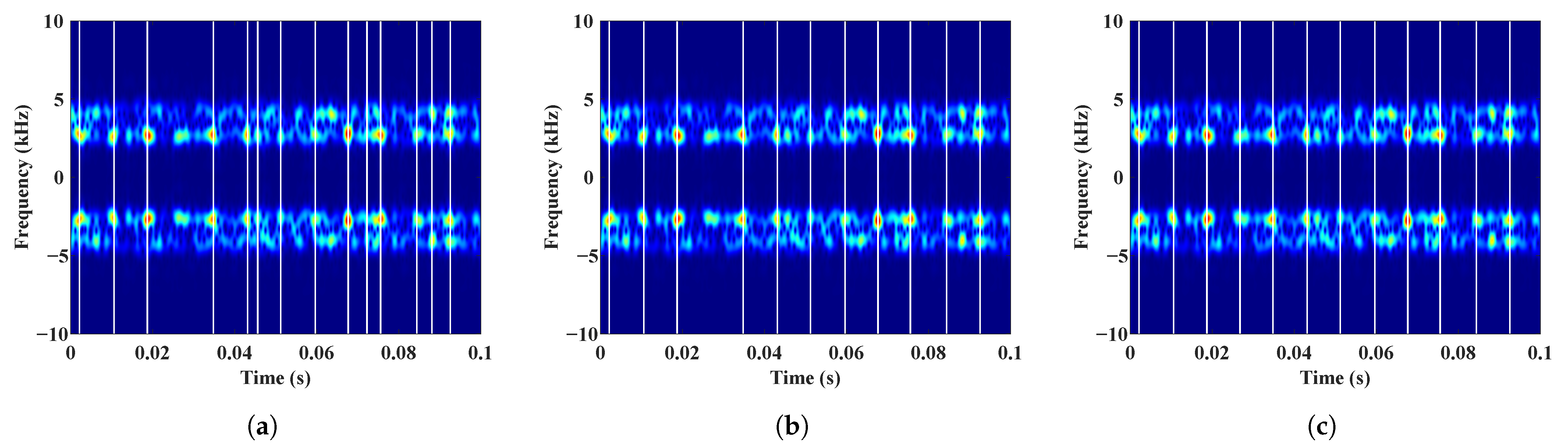
The simulation also adopts the state of the drone set in Table 1. Figure 4 shows the change of the time domain echo time–frequency spectrum of the single rotor with the attitude of the drone and Figure 5 offers the time–frequency spectrum of the quad-rotor in different states. Compared to Figure 2, it can be seen that the essential features of the electromagnetic simulation and the theoretical simulation are entirely consistent, which proves the reliability of the previous theoretical simulation analysis results.

3. Micro-Motion Parameter Estimation Algorithm Based on CVMD and SVD

For the micro-Doppler signature of multi-rotor drones, the flicker corresponding to each rotor is very likely to have aliasing. It is unrealistic to extract micro-motion parameters from the flicker with severe aliasing. The proposed algorithm takes the two groups of flickers with different frequencies, shown in Figure 5c and d; the basic process of parameter extraction is demonstrated in Figure 6. When the flickering of the quad-rotors can be distinguished, it is only necessary to make a distinction after the high and low-frequency flickers are completed (not considered in this study). In addition, the target translational motion will cause the echo signal to produce a Doppler frequency shift. At present, the mainstream method uses translation compensation to remove the influence of the target translation [19,28,29]. The algorithm in this paper is aimed at the signal that has undergone translation compensation.

3.1. CVMD Frequency Domain Segmentation

VMD was first proposed in [30], a solution process for the variational problem based on the Wiener filter, Hilbert transform, and mixed frequencies. It is assumed that the target signal consists of a specified number of band-limited intrinsic mode functions (BLIMFs) $u_k$, each of which corresponds to a center frequency ${\omega }_k$ and is closely clustered around the respective center frequency. Therefore, the key to realizing VMD is solving each mode’s center frequency and bandwidth. The calculation result is affected by the number of decomposition layers K. The basic idea of this method is to transform the solution process of the modal bandwidth and central frequency into a constrained optimization process. The original signal is finally transformed into K BLIMFs with special sparsity and independence by iteratively searching for the optimal solution of the constrained variational model.

In view of the characteristic that VMD decomposes the signal according to the center frequency, this paper proposes using VMD to separate the high-frequency components of the high-frequency flicker in the echo signal separately. Referring to the basic principle of VMD, the VMD solution process needs to first perform the Hilbert transform on the original signal. However, the Hilbert transform can only be applied to process and preserve the complete information of the real signal. For a complex signal whose spectrum is single-sided and asymmetric, such as radar echo, half of the spectrum structure of the reconstructed signal would be lost after the Hilbert transform. Therefore, the VMD cannot directly process the radar echo signal.

In response to the defect that VMD cannot directly handle complex signals, the authors of [31,32] extended the empirical mode decomposition (EMD) method to the complex domain and successfully realized the VMD reconstruction of complex signals. The basic process of decomposing and reconstructing radar echo signals concerning CVMD is shown in Figure 7. The number of decomposed modes K needs to be modified according to different target signals.

Using the above CVMD reconstruction process, the signal is decomposed into K BLIMFs $\{u_1,u_2,\cdots ,u_K\}$, and each BLIMF will correspond to a different center frequency. At this time, the spectrum obtained by FT or the time–frequency spectrum obtained by STFT can be used to sort the BLIMF according to the size of the center frequency. In this paper, the time–frequency spectrum is used to analyze the center frequency to facilitate the selection of suitable BLIMFs for combination. Finally, the frequency domain segmentation of the signal can be completed by combining the BLIMFs according to the desired purpose.

3.2. SVD Time Domain Positioning

SVD is a well-known technical means. It can be used to reduce the cross-terms in the high-resolution time–frequency distributions. It can also use the obtained singular vector as the target feature to reduce the dimension of the feature space. There are many applications in classifying “low, small, slow” objects [25,33,34]. The SVD of matrix M can be expressed as

$$M=U\Sigma V^T.$$

(13)

Among them, $\mathrm{\Sigma }$ is a diagonal matrix, the diagonal elements correspond to the singular values of X, and U and V represent the left singular vector and the right singular vector, respectively.

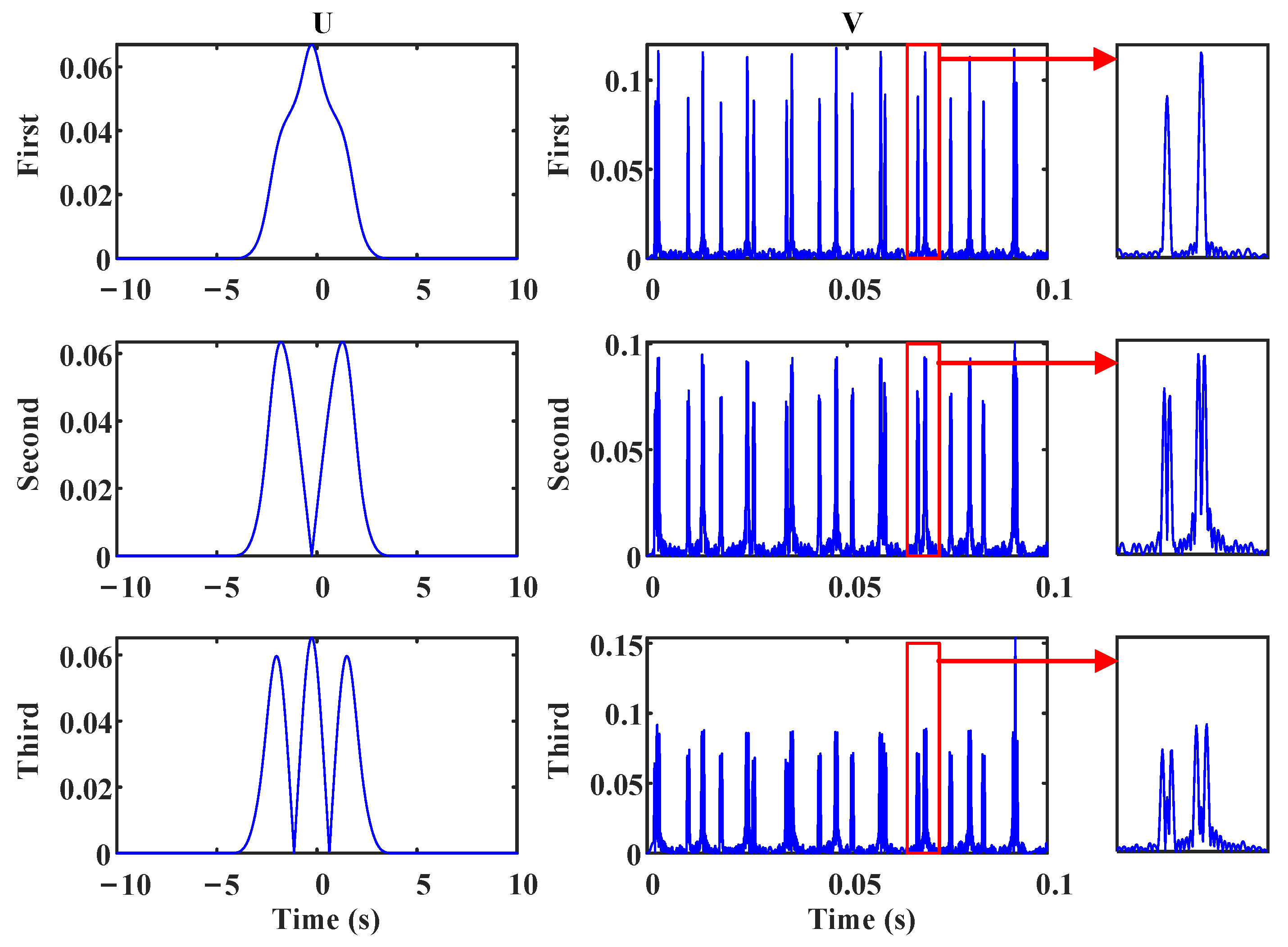
Reference [34] shows that if SVD is used for a complete time–frequency spectrum, the time and frequency information of the original spectrogram will be decoupled and projected onto the left singular vector and the right singular vector. At this time, the left singular vector U will represent the frequency information of the spectrogram, and the right singular vector V will be able to represent the time information of the spectrogram.

Considering that the singular vectors obtained by SVD are arranged according to the corresponding eigenvalues from large to small, most of the information in the time spectrum is contained in the first few singular vectors. The first three singular vectors obtained using the spectral matrix SVD of Figure 2f are shown in Figure 8. The results show that the left singular vectors can roughly reflect the micro-Doppler frequency range of the flicker band, and the frequency domain ranges of the first three left singular vectors are roughly the same. The peak of the right singular vector protrusion is very close to the time domain position of each flicker in the time–frequency spectrum. The first right singular vector is the most obvious, and the second and third right singular vectors will form multiple bifurcations near the peak of the first singular vector, which is very unfavorable for the extraction of the peak time domain position. Under careful consideration, the first singular vector obtained by SVD is applied to analysis and research.

In order to obtain the temporal position of the flicker directly from the right singular vector, a thresholded peak detection method is proposed. First, a Gaussian smoothing process is performed on the first right singular vector to prevent the influence of individual Burr points to the extraction results. The length of the Gaussian smoothing window should not be too large to ensure that the influence on the elements in the original vector is minimized. Then adopt the method of peak detection to detect all the peak points in the first right singular vector. Assuming that the numerical sequence of singular vectors is $\left\{x_1,x_2,\cdots ,x_n\right\}$, calculate the difference between adjacent elements $\mathrm{\Delta }{x}_i$

$$\mathrm{\Delta }{x}_i=x_{i+1}-x_i,i=1,2,\cdots ,n-1.$$

(14)

$$\mathrm{\Delta }{x}_i>0;\mathrm{\Delta }{x}_{i+1}<0.$$

(15)

When Equation (15) is satisfied, the element can be determined as the peak point. Finally, the non-target points are eliminated through the threshold, and the threshold $Th$ is set as

$$Th=\delta ·max\left(V_1\right).$$

(16)

Among them, $\delta$ is the threshold factor, which needs to be adjusted according to the strength of the error component, generally taking 0.6. $V_1$ is the first right singular vector, and $max\left(V_1\right)$ represents the maximum value of $V_1$. The thresholding analysis method is widely used in digital image processing, and it will also be used in the subsequent estimation of flicker micro-Doppler parameters.

3.3. Process of the Algorithm

Combined with CVMD frequency domain segmentation and SVD time domain positioning, extracting the micro-Doppler parameters of multi-rotor targets will be straightforward. The specific steps of the proposed algorithm are as follows:

• Signal frequency domain segmentation and reconstruction. Select the appropriate number of decomposition layers K to perform CVMD frequency domain segmentation on the signal. Decompose the signal into three parts: body component, high-frequency component, and intermediate frequency component, where the intermediate frequency component is the sum of the functions of the residual mode, except the high-frequency component and the body component.
• Flicker time domain positioning. Using the SVD time domain positioning method proposed in Section 3.2, the complete flicker time domain coordinate set A and the high-frequency flicker time domain coordinate set B are obtained from the intermediate frequency and high-frequency components.
• High-frequency flicker time domain coordinate correction. Calculate the distance between the adjacent coordinate elements $\mathrm{\Delta }B$.

$$\begin{array}{cc}\hfill \mathrm{\Delta }B& =\left\{\mathrm{\Delta }{b}_1,\cdots ,\mathrm{\Delta }{b}_{n-1}\right\}\hfill \\ \hfill & =\left\{b_2-b_1,\cdots ,b_n-b_{n-1}\right\},b_1,\cdots b_n\in B,\hfill \end{array}$$

(17)

where $b_i,i=1,\cdots ,n$ are all elements in set B, and n is the number of elements in the coordinate set.

If $\left|max\left(\mathrm{\Delta }B\right)-min\left(\mathrm{\Delta }B\right)\right|>1.1·min\left(\mathrm{\Delta }B\right)$, it is considered that there is a wrong positioning point; execute $1)$ to set the erroneous points deleted. If $\left|max\left(\mathrm{\Delta }B\right)-min\left(\mathrm{\Delta }B\right)\right|>1.1·min\left(\mathrm{\Delta }B\right)$, it means that there is no wrong positioning point in set B; it is necessary to complete the possible missing points in set B and execute b. If the b execution condition is established, then loop a operation until the b operation condition is satisfied, and then execute b. The flowchart of this time domain coordinate correction process is shown in the Figure 9.

(a)

Solve for the label $E_k$ of the wrong coordinate in B, and delete the coordinate element $b_{E_k}$ in set B.

$$E_k=\left\{\begin{array}{c}arg\left(\mathrm{\Delta }{b}_{argmin\left(\mathrm{\Delta }B\right)-1}\right)+1,\mathrm{\Delta }{b}_{argmin\left(\mathrm{\Delta }B\right)-1}<\mathrm{\Delta }{b}_{argmin\left(\mathrm{\Delta }B\right)+1}\hfill \\ arg\left(\mathrm{\Delta }{b}_{argmin\left(\mathrm{\Delta }B\right)+1}\right)-1,\mathrm{\Delta }{b}_{argmin\left(\mathrm{\Delta }B\right)-1}\ge \mathrm{\Delta }{b}_{argmin\left(\mathrm{\Delta }B\right)+1}\hfill \end{array}\right.$$

(18)

(b)

Calculate the coordinate interval evaluation factor ${\zeta }_i$

$${\zeta }_i=[\mathrm{\Delta }{b}_i/min\left(\mathrm{\Delta }B\right)],i=1,\cdots ,n-1$$

(19)

where $\left[·\right]$ means approximate rounding. If ${\zeta }_i>1$, add ${\zeta }_i-1$ elements between $b_i$ and $b_{i+1}$ to make the interval $\left[b_i,b_{i+1}\right]$ do ${\zeta }_i$ equal division, and update set B. After completing all missing supplementary points, use the mean value of $\mathrm{\Delta }B$$\mathrm{\Delta }\overline{B}$ to determine whether there are elements missing at the left and right ends of the set, and if so, use $\mathrm{\Delta }\overline{B}$ as an interval to complete the missing elements.

4.

High-frequency flicker micro-Doppler parameter estimation. The $\mathrm{\Delta }\overline{B}$ solved after the correction in step 2 is the estimated value of the flicker interval. In addition, in order to solve the Doppler bandwidth of the flicker, calculate the sum of $F{S}_B$ of the $5n$ frequency domain vectors with a radius of 2 and all time domain coordinates in B

$$F{S}_B=\sum _{i=1}^n\sum _{k=b_i-2}^{b_i+2}T{F}_{f_k},$$

(20)

where $T{F}_{f_k}$ represents the frequency domain vector whose time domain coordinate is k in the time–frequency spectrum. Then do the same threshold segmentation as formula Equation (16) with the vector $F{S}_B$. At this time, the threshold generally takes $\delta =0.5$. After segmentation, the frequency domain width of a high-frequency flicker is the estimated value of its Doppler bandwidth $B_{BW}$.

$$B_{BW}=max\left(arg\left(F{S}_B>\delta ·max\left(F{S}_B\right)\right)\right)-min\left(arg\left(F{S}_B>\delta ·max\left(F{S}_B\right)\right)\right).$$

(21)

5.

The nearest neighbors difference set. Delete the point $a_{argmin\left(\left|A-b_i\right|\right)}$ in set A that is closest to the element position in set B to obtain a low-frequency flickering time domain coordinate set C.

6.

Low-frequency flicker micro-Doppler parameter estimation.

(a)

Use the same method as step 3b to process set B to complete the missing points of set C.

(b)

Use the method of step 4 to estimate the micro-Doppler parameters $C_{BW}$ and $\mathrm{\Delta }\overline{C}$ of low-frequency flicker. In order to avoid the influence of the high-frequency flicker on the estimation result of the low-frequency flicker Doppler bandwidth, the flicker point set $C_0$, which is relatively far away from the high-frequency flicker in set C is selected to estimate the Doppler bandwidth. Calculate the point $a_{argmin\left(\left|C-b_i\right|\right)}$ and the corresponding shortest distance $min\left(\left|C-b_i\right|\right)$, delete all points in set C that satisfy Equation (22) to obtain set $C_0$.

$$min\left(\left|C-b_i\right|\right)<len/2,$$

(22)

in which $len$ means the window length used in STFT.

(c)

In order to prevent periodic missing in low-frequency flicker coordinate positioning results—use to replace ${\zeta }_i$ as the interval evaluation factor to perform the step 3b operation to make a second correction to set C.

$${\zeta }^{\prime }=\frac{B_{BW}·\mathrm{\Delta }\overline{B}}{C_{BW}·\mathrm{\Delta }\overline{C}}.$$

(23)

7.

Micro-motion parameter estimation. Referring to Equations (8) and (10), the rotor blade rotational frequency $f_r$ and blade length L can be estimated

$$f_r=f_s/(N·\mathrm{\Delta }\overline{X}),$$

(24)

$$L=\lambda X_{BW}/8\pi f_{r}cos\theta ,$$

(25)

where $f_s$ represent the pulse repetition frequency, $\mathrm{\Delta }\overline{X}$ and $X_{BW}$ represent the estimated flicker interval and flicker Doppler bandwidth of the two groups of flickers.

4. Results

4.1. Analysis of Algorithm Simulation

The proposed algorithm’s purpose and the theoretical parameter estimation process have been shown in the previous subsection. In this section, we will verify the algorithm’s effectiveness for estimating micro-motion parameters of multi-rotor targets. In addition, to demonstrate the specific signal processing process by the proposed algorithm, the processing process of each step of the algorithm is analyzed and displayed by taking the electromagnetic simulation results; see Figure 5c as an example.

The proposed algorithm firstly performs CVMD frequency domain segmentation on the signal after translation compensation. The key to this process is to select the appropriate number of decomposition layers K to decompose and reconstruct the original signal. In order to improve efficiency, the minimum number of decomposition layers that can separate high-frequency components is generally selected for processing. After frequency domain segmentation, the modal functions can be combined according to the time–frequency spectrum obtained by the modal function STFT. The signal will be divided into three parts: body component, high-frequency component, and intermediate frequency component. The time–frequency spectrum of the three components is shown in Figure 10.

At this time, the SVD time domain positioning of Figure 10b,c can be used to obtain the complete flicker and the high-frequency flicker coordinate set corresponding to the flicker in the figure. The body component is separated when performing frequency domain segmentation to reduce the influence of the body component on flicker positioning. In general, the electromagnetic scattering of the body is much stronger than that of the blades, and the flicker feature in the right singular vector obtained by SVD is easily overwhelmed by the body component. Moreover, the more significant the difference between the scattering intensity of the body component and the rotor component, the more serious the contamination will be. Figure 11 shows the comparison of the first singular vector obtained before and after removing the body component. The results show that if the body component is not removed, the convex peak characterizing the flicker feature in the first right singular vector will be completely contaminated.

As shown in Figure 10c, the high-frequency components contain very few signal components. When the signal-to-noise ratio (SNR) is low, the signal pollution’s influence on the time domain localization of the high-frequency flicker will be more obvious. If the coordinate set obtained from the high-frequency components is not preprocessed, the anti-noise ability of the entire parameter extraction algorithm will be significantly reduced. Figure 12a shows the flicker time domain coordinates of the high-frequency components acquired at an SNR of -2dB. Due to noise pollution, the flicker time domain location results have false detection points and missing points. The algorithm proposed in this paper adds step 3 to correct the obtained high-frequency flickering coordinates. After the first correction, the wrong coordinates will be removed (see Figure 12a). The second correction step is then performed to supplement the missed coordinates, and the final flicker coordinates detection result is shown in Figure 12c. After testing, the proposed correction strategy can obtain the correct flicker time domain coordinates as long as the obtained coordinates reflect the periodic flicker without continuous missing.

The time domain coordinates of all low-frequency flickers except the aliasing flicker can be obtained through the nearest neighbor difference processing of the time domain coordinate sets of complete and high-frequency flickers. Figure 13 shows the effects of marking the high-frequency flicker coordinates and the low-frequency flicker coordinates in the time–frequency spectrum of the original signal. Due to the influence of aliasing flicker, the low-frequency flicker obtained after the difference set will be partially missing. At this time, it is also necessary to correct the low-frequency flicker coordinate set. Since the differentiated intermediate frequency components have a much more significant proportion than the high-frequency components in the original signal, its noise adaptability is more robust than the high-frequency flicker localization. On the premise that the coordinates of the high-frequency flicker can be accurately extracted, and the location results of the full flicker coordinates are accurate. The correction to the coordinates of the low-frequency flicker is aimed at complementing the missing coordinates of the aliased flicker.

After obtaining the complete flicker time domain position, the estimation of micro-Doppler parameters can be completed according to steps 4 and 6 of the proposed algorithm. Figure 14 shows the flicker reconstruction results obtained using the estimated micro-Doppler parameters. Observing the two aliased flickering areas originally in Figure 13, we found the double flickering areas in the original flickering area, which were both correctly reconstructed.

4.2. Results of Parameter Estimation

In addition to the most apparent flicker, the micro-Doppler characteristics of multi-rotor targets also have sinusoidal envelopes that represent the Doppler characteristics of the blade tip scattering points. The number of these sinusoids corresponds to the number of blades. Combined with the micro-Doppler curve of the flicker parameters, such as the range, the blade rotation period, and the time domain position of the initial flicker, the reconstruction of these sinusoidal envelopes can be realized. Using high-frequency flickering envelopes as an example, the mathematical expression $f_{envelope}$ can be expressed as

$$f_{en}=\pm B_{BW}sin\left(2\pi f_r(t+b_1)+\pi /2\right)$$

(26)

Figure 15 shows the effect of drawing the reconstructed flicker and sinusoidal envelope of Figure 4c and d in the original time–frequency spectrum. It is observed that the reconstructed micro-Doppler curve is in good agreement with the micro-Doppler signatures in the original time–frequency spectrum. In order to compare the accuracy of the final extraction results,

Table 2. Micro-Doppler parameter estimation and real value comparison.

		Type 6		Type 8
		Estimated Value	Actual Value	Estimated Value	Actual Value
Flickering cycle (ms)	High-frequency flicker	8.2500	8.1967	6.2467	6.2500
	Low-frequency flicker	11.1000	11.1111	8.3500	8.3333
Rotor rotation frequency (Hz)	High-frequency flicker	60.6061	61.0000	80.0427	80.0000
	low-frequency flicker	45.0450	45.0000	59.8892	60.0000
Doppler bandwidth (kHz)	High-frequency flicker	6.3332	6.2632	4.7824	4.7424
	low-frequency flicker	4.5723	4.6204	3.6618	3.5568
Blade length (m)	High-frequency flicker	0.1439	0.1414	0.1425	0.1414
	Low-frequency flicker	0.1398	0.1414	0.1459	0.1414

lists the comparison between the estimated and actual values of the fretting parameters obtained using Figure 4c,d. The results show that the proposed algorithm accurately estimates the micro-motion parameters.

5. Discussions

5.1. The Influence of Noise on Parameter Estimation

To evaluate the robustness of the proposed algorithm, we test the algorithm’s probability of correctly detecting the localization flicker at different SNRs and the accuracy of parameter estimation. The test uses the theoretical simulation results of type 6 and type 7 in Table 1 for parameter estimation and performs 100 Monte Carlo experiments on the simulated signals under each SNR. The proposed algorithm relies on the ability of SVD to locate the flicker time domain location. The SVD time domain location includes the high-frequency flicker time domain location of the high-frequency component and the intermediate frequency component’s complete flicker time domain location. We also counted the correct detection probability (CDP) of these two flicker localizations. Figure 16 shows the probability statistics of complete flicker localization, high-frequency flicker localization, and the final reconstruction of all flickers in the parameter estimation process. The results show that the proposed algorithm can complete the flicker reconstruction when the signal SNR is larger than −2 dB.

Figure 17 shows the mean relative error (MRE) statistics of the rotor rotating frequency, the flicker Doppler bandwidth, and blade length estimation by the proposed algorithm under different SNRs, in which the parameter estimation results that correctly complete the flicker reconstruction are selected for the error evaluation. The blade length estimate of the algorithm is calculated from the flicker period and Doppler bandwidth estimation results. Since the estimated flicker period accuracy can be very high when the flicker is correctly located, the primary source of error in the blade length estimation is the Doppler bandwidth estimation. Therefore, the MRE of the two groups of rotor blade lengths in Figure 17 are consistent with the Doppler bandwidth estimation results. With a comprehensive analysis of the CDP and MRE statistical results, the algorithm can effectively accomplish the micro-motion parameter estimation when the SNR is larger than −2 dB.

5.2. Strengths and Weaknesses

As summarized in the following paragraphs, this paper’s main strengths can be summed up as follows:

(1)

This paper analyzes the relationship between the multi-rotor micro-Doppler characteristics and the initial position of the rotor in detail. This work will provide a specific theoretical basis for researching the multi-rotor target micro-Doppler characteristics.

(2)

The proposed CVMD frequency domain segmentation method broadens the application of VMD in radar signal processing. According to the basic idea of the proposed method, the signal with obvious frequency domain distinction can be divided into frequency domains according to different purposes.

(3)

The proposed SVD time domain localization method can quickly obtain the time domain position of the flicker in the time–frequency spectrum. This method can be extended to the feature extraction of time domain images with obvious time domain distinction.

(4)

The proposed method can directly and automatically obtain the micro-Doppler parameter information of the multi-rotor target without other redundant operations, which makes up for the problem that the existing non-parametric parameter estimation methods are difficult to obtain the complete parameters of the multi-rotor.

In addition, the method proposed in this paper has some shortcomings, mainly the following:

(1)

The frequency domain segmentation idea of CVMD relies on the stable frequency domain distinction of the signal. When the position of the target signal in the frequency domain changes according to time, the frequency domain segmentation effect of this method will decrease rapidly.

(2)

Generally, the rotor speed difference of the multi-rotor drone is not particularly large, and the extracted high-frequency components will contain very few signal components. Therefore, the signal-to-noise ratio that the proposed method can adapt to is limited.

(3)

Although the proposed method solves the flicker reconstruction in the case of weak aliasing, the aliasing situation will be dire when there are many flicker components. Therefore, it was necessary for us to introduce a time–frequency analysis method with higher resolution (especially temporal resolution) in the following research.

6. Conclusions

For the multi-rotor target, this paper uses the scattering point integral model to complete the construction of the theoretical echo mathematical model of the rotor drone. It completes the analysis and verification of the multi-rotor drone flicker characteristics through theoretical and electromagnetic simulations. Regarding the difficulties brought by the multi-rotor and multi-speed multi-rotor drone in estimating the micro-motion parameters, this paper takes a non-parametric parameter estimation method based on CVMD and SVD. The simulation results show that the proposed algorithm can successfully extract the micro-motion parameters of the multi-rotor target. Finally, to test the performance of the proposed algorithm, the probability of correctly detecting the position of the flicker in the time domain and the error of the parameter estimation under different SNRs were statistically analyzed. Tests show that the algorithm can complete the stable estimation of micro-motion parameters when the SNR is larger than −2dB. In follow-up research, we will consider studying the use of Doppler features of drone targets to classify their motion states. At this point, we can obtain the movement trend of the target to evaluate its risk factor. Thus, effective response strategies can be formulated in advance to avoid accidents with potential threat targets. This work will provide technical support for preventing and controlling rotary-wing drones.

References

- Fan, B.; Li, Y.; Zhang, R.; Fu, Q. Review on the technological development and application of UAV systems. Chin. J. Electron. 2020, 29, 199–207. [Google Scholar] [CrossRef]
- Gong, J.; Yan, J.; Li, D.; Kong, D.; Hu, H. Interference of Radar Detection of Drones by Bird. Prog. Electromagn. Res. M 2019, 81, 1–11. [Google Scholar] [CrossRef] [Green Version]
- Chen, V.C.; Qian, S. Joint time-frequency transform for radar range-Doppler imaging. IEEE Trans. Aerosp. Electron. Syst. 1998, 34, 486–499. [Google Scholar] [CrossRef]
- Zhao, C.; Luo, G.; Wang, Y.; Chen, C.; Wu, Z. UAV Recognition Based on Micro-Doppler Dynamic Attribute-Guided Augmentation Algorithm. Remote Sens. 2021, 13, 1205. [Google Scholar] [CrossRef]
- Hanif, A.; Muaz, M.; Hasan, A.; Adeel, M. Micro-Doppler based Target Recognition with Radars: A Review. IEEE Sens. J. 2022, 22, 2948–2961. [Google Scholar] [CrossRef]
- Chen, X.; Zhang, H.; Song, J.; Guan, J.; Li, J.; He, Z. Micro-Motion Classification of Flying Bird and Rotor Drones via Data Augmentation and Modified Multi-Scale CNN. Remote Sens. 2022, 14, 1107. [Google Scholar] [CrossRef]
- Ritchie, M.; Fioranelli, F.; Griffiths, H. Monostatic and bistatic radar measurements of birds and micro-drone. In Proceedings of the 2016 IEEE Radar Conference (RadarConf), Philadelphia, PA, USA, 2–6 May 2016. [Google Scholar] [CrossRef] [Green Version]
- Rahman, S.; Robertson, D.A. Radar micro-Doppler signatures of drones and birds at K-band and W-band. Sci. Rep. 2018, 8, 17396. [Google Scholar] [CrossRef] [PubMed]
- Tahmoush, D. Detection of Small UAV Helicopters Using Micro-Doppler. In Proceedings of the SPIE Defense + Security, Baltimore, MD, USA, 29 May 2014. [Google Scholar] [CrossRef]
- Fang, X.; Lu, C.; Zhang, M.; Min, R. Detection of Small UAV Helicopters Using Micro-Doppler. In International Conference in Communications, Signal Processing, and Systems; Springer: Singapore, 2017. [Google Scholar] [CrossRef]
- Chen, J.; Zhang, J.; Jin, Y.; Yu, H.; Liang, B.; Yang, D.G. Real-Time Processing of Spaceborne SAR Data with Nonlinear Trajectory Based on Variable PRF. IEEE Trans. Geosci. Remote Sens. 2021, 60, 1–12. [Google Scholar] [CrossRef]
- Chen, V.C.; Li, F.; Ho, S.-S.; Wechsle, H. Micro-Doppler effect in radar: Phenomenon, model, and simulation study. IEEE Trans. Aerosp. Electron. Syst. 2006, 42, 2–21. [Google Scholar] [CrossRef]
- Torvik, B.; Olsen, K.E.; Griffiths, H. Classification of Birds and UAVs Based on Radar Polarimetry. IEEE Geosci. Remote Sens. Lett. 2016, 13, 1305–1309. [Google Scholar] [CrossRef]
- Li, T.; Wen, B.; Tian, Y.; Wang, S.; Yin, Y. Optimized Radar Waveform Parameter Design for Small Drone Detection Based on Echo Modeling and Experimental Analysis. IEEE Access 2019, 7, 101527–101538. [Google Scholar] [CrossRef]
- Schröder, A.; Aulenbacher, U.; Renker, M.; Böniger, U.; Oechslin, R.; Murk, A.; Wellig, P. Numerical RCS and micro-Doppler investigations of a consumer UAV. In Proceedings of the SPIE Security + Defence, Edinburgh, UK, 24 October 2016. [Google Scholar] [CrossRef]
- Speirs, P.J.; Schröder, A.; Renker, M.; Wellig, P.; Murk, A. Comparisons between simulated and measured X-band signatures of quad-, hexa-and octocopters. In Proceedings of the 15th European Radar Conference (EuRAD), Madrid, Spain, 29 November 2018. [Google Scholar] [CrossRef]
- Li, Y.; Yi, J.; Wan, X.; Liu, Y.; Zhan, W. Helicopter rotor parameter estimation method for passive radar. J. Radars 2018, 7, 313–319. [Google Scholar] [CrossRef]
- Zhou, Z.; Zhang, C.; Xia, S.; Xu, D.; Gao, Y.; Zeng, X. Feature Extraction of Rotor Blade Targets Based on Phase Compensation in a Passive Bistatic Radar. J. Radars 2021, 10, 929–943. [Google Scholar] [CrossRef]
- Ji, G.; Song, C.; Huo, H. Detection and identification of low-slow-small rotor unmanned aerial vehicle using micro-Doppler information. IEEE Access 2021, 9, 99995–100008. [Google Scholar] [CrossRef]
- Liu, J.; Ai, X.; Feng, Z.; Wu, Q. Motion estimation of micro-motion targets with translational motion. In Proceedings of the IET International Radar Conference 2015, Hangzhou, China, 14–16 October 2015. [Google Scholar] [CrossRef]
- Gannon, Z.; Tahmoush, D. Measuring UAV propeller length using micro-Doppler signatures. In Proceedings of the IEEE International Radar Conference (RADAR), Washington, DC, USA, 28–30 April 2020. [Google Scholar] [CrossRef]
- Zhang, W.; Li, G. Detection of Multiple Micro-Drones via Cadence Velocity Diagram Analysis. Electron. Lett. 2018, 54, 441–443. [Google Scholar] [CrossRef]
- Kang, K.; Choi, J.; Cho, B.; Lee, J.; Kim, K. Analysis of micro-Doppler signatures of small UAVs based on Doppler spectrum. IEEE Trans. Aerosp. Electron. Syst. 2021, 57, 3252–3267. [Google Scholar] [CrossRef]
- Wu, Q.; Zhao, J.; Zhang, Y.; Huang, Y. Radar Micro-Doppler Signatures Model Simulation and Feature Extraction of Three Typical LSS Targets. In Proceedings of the International Conference on Information Science and Control Engineering (ICISCE), Shanghai, China, 20–22 December 2019. [Google Scholar] [CrossRef]
- Harmanny, R.I.A.; de Wit, J.J.M.; Prémel Cabic, G. Radar micro-Doppler feature extraction using the spectrogram and the cepstrogram. In Proceedings of the 11th European Radar Conference, Rome, Italy, 18 December 2014. [Google Scholar] [CrossRef] [Green Version]
- Song, C.; Zhou, L.; Wu, Y.; Ding, C. An Estimation Method of Rotation Frequency of Unmanned Aerial Vehicle Based on Auto-correlation and Cepstrum. J. Electron. Inf. Technol. 2019, 41, 255–261. [Google Scholar] [CrossRef]
- Huizing, A.; Heiligers, M.; Dekker, B.; de Wit, J.J.M.; Cifola, L.; Harmanny, R. Deep Learning for Classification of Mini-UAVs Using Micro-Doppler Spectrograms in Cognitive Radar. IEEE Aerosp. Electron. Syst. Mag. 2019, 34, 46–56. [Google Scholar] [CrossRef]
- Gu, F.F.; Fu, M.H.; Liang, B.S.; Li, K.M.; Zhang, Q. Translational motion compensation and micro-Doppler feature extraction of space spinning targets. IEEE Geosci. Remote Sens. Lett. 2018, 15, 1550–1554. [Google Scholar] [CrossRef]
- Chen, J.; Yu, H.; Liang, B.; Peng, J.; Sun, G.C. Motion compensation/autofocus in airborne synthetic aperture radar: A review. IEEE Geosci. Remote Sens. Mag. 2021, 10, 1109. [Google Scholar] [CrossRef]
- Dragomiretskiy, K.; Zosso, D. Variational mode decomposition. IEEE Trans. Signal Process. 2013, 62, 531–544. [Google Scholar] [CrossRef]
- Wang, Y.; Liu, F.; Jiang, Z.; He, S.; Mo, Q. Complex variational mode decomposition for signal processing applications. Mech. Syst. Signal Process. 2017, 86, 75–85. [Google Scholar] [CrossRef]
- Tanaka, T.; Mandic, D.P. Complex empirical mode decomposition. IEEE Signal Process. Lett. 2007, 14, 101–104. [Google Scholar] [CrossRef]
- De Wit, J.J.M.; Harmanny, R.I.A.; Molchanov, P. Radar micro-Doppler feature extraction using the Singular Value Decomposition. In Proceedings of the 2014 International Radar Conference, Lille, France, 13–17 October 2014. [Google Scholar] [CrossRef]
- Ritchie, M.; Fioranelli, F.; Borrion, H.; Griffiths, H. Multistatic micro-Doppler radar feature extraction for classification of unloaded/loaded micro-drones. IET Radar Sonar Navig. 2017, 11, 116–124. [Google Scholar] [CrossRef] [Green Version]
Figure 1.
The geometric relationship between the radar and drone.
Figure 2.
Drone echo time–frequency spectrum in different states. (a) Type 1. (b) Type 2. (c) Type 3. (d) Type 4. (e) Type 5. (f) Type 6. (g) Type 7. (h) Type 8.
Figure 3.
The 3D model of drone electromagnetic simulation.
Figure 4.
Blade spin time–frequency spectrum electromagnetic simulation in different radar observation angles (Type 1). (a) . (b) . (c) . (d) .
Figure 5.
Drone time–frequency spectrum electromagnetic simulation in different states. (a) Type 2. (b) Type 4. (c) Type 6. (d) Type 8.
Figure 6.
Basic process of multi-rotor micro-motion parameter extraction. In which HF means high-frequency, IF means intermediate frequency, and LF means low-frequency.
Figure 7.
Basic process of radar echo CVMD reconstruction.
Figure 8.
The first three singular vectors of the spectral matrix SVD.
Figure 9.
Process of the high-frequency flicker time domain coordinate correction.
Figure 10.
The three components obtained by CVMD. (a) Body component. (b) Intermediate frequency component. (c) High-frequency component.
Figure 11.
The first singular vector comparison before and after removal of the body component signal.
Figure 12.
High-frequency flicker correction schematic diagram. (a) Before correction. (b) First correction. (c) Complete correction.
Figure 13.
Time–frequency spectrum full flashing time domain location tag diagram.
Figure 14.
Figure 15.
High-frequency flicker correction schematic diagram. (a) Figure 5c reconstruction result. (b) Figure 5d reconstruction result.
Figure 16.
CDP of the SVD time domain location.
Figure 17.
The average relative error of the parameter estimation under a different SNR. FRRF stands for flicker rotor rotating frequency, FDB stands for flicker Doppler bandwidth, and RBL stands for rotor blade length.