
Spatial and Spectral-Channel Attention Network for Denoising on Hyperspectral Remote Sensing Image

1
School of Science, Xihua University, Chengdu 610039, China
2
School of Information Engineering, Zhejiang Ocean University, Zhoushan 316022, China
3
Key Laboratory of Oceanographic Big Data Mining and Application of Zhejiang Province, Zhoushan 316022, China
4
School of Mathematical Sciences, University of Electronic Science and Technology of China, Chengdu 611731, China
*
Author to whom correspondence should be addressed.
Remote Sens. 2022, 14(14), 3338; https://0-doi-org.brum.beds.ac.uk/10.3390/rs14143338
Submission received: 28 May 2022
/
Revised: 3 July 2022
/
Accepted: 7 July 2022
/
Published: 11 July 2022
(This article belongs to the Special Issue Machine Vision and Advanced Image Processing in Remote Sensing)
Abstract
:Hyperspectral images (HSIs) are frequently contaminated by different noises (Gaussian noise, stripe noise, deadline noise, impulse noise) in the acquisition process as a result of the observation environment and imaging system limitations, which makes image information lost and difficult to recover. In this paper, we adopt a 3D-based SSCA block neural network of U-Net architecture for remote sensing HSI denoising, named SSCANet (Spatial and Spectral-Channel Attention Network), which is mainly constructed by a so-called SSCA block. By fully considering the characteristics of spatial-domain and spectral-domain of remote sensing HSIs, the SSCA block consists of a spatial attention (SA) block and a spectral-channel attention (SCA) block, in which the SA block is to extract spatial information and enhance spatial representation ability, as well as the SCA block to explore the band-wise relationship within HSIs for preserving spectral information. Compared to earlier 2D convolution, 3D convolution has a powerful spectrum preservation ability, allowing for improved extraction of HSIs characteristics. Experimental results demonstrate that our method holds better-restored results than other compared approaches, both visually and quantitatively.
1. Introduction
Numerous continuous bands are present in each spatial position of the natural scene in hyperspectral images (HSIs), from visible band to infrared band, and are rich in spatial and spectral information, providing richer scene information than RGB images.
The high representation ability of HSIs can substantially increase how well perform in computer vision tasks , such as classification [1,2], detection [3], tracking [4] and unmixing [5,6]. However, real-world HSIs are frequently tainted by different noises [7] (such Gaussian noise, stripe noise, and impulse noise) in the acquisition process [8], because of the restrictions of the observing environment and imaging system. These annoying noises limit the performance of all of the above processing tasks. Therefore, HSI denoising has become an essential pretreatment for HSI applications and has attracted extensive attention. And our visual result is shown in Figure 1.
A large number of denoising methods for HSIs have been proposed until now, which may be roughly divided into two categories, i.e., traditional methods and deep learning (DL)-based methods. The traditional methods, mainly including filtering-based techniques and optimization-based techniques, are dominated in the early period. As one of the most famous filtering-based techniques, BM3D [10] realizes the amazing 2D image denoising results by block-matching and filtering strategies. Extending the idea of BM3D, BM4D [11] may be directly applied to HSI denoising with the similar block-matching and filtering strategies. Peng et al. proposed a method for tensor dictionary learning (TDL) model [12], allowing consideration of global correlation along spectral (GCS) and non-local self-similarity (NSS) in HSIs, and achieved good performance. On this basis, low-rank tensor-based, ITS-REG [13], and LLRT models [14], as well as a new iterative projection denoising algorithm NMoG [9], were proposed. They explored the inherent characteristics of HSIs and conducted fine modeling, and further ameliorated the denoising effect. These methods take into account potential features in HSIs to achieve denoising results. However, because they rely on human cognition and observation, they may be limited by inaccurate priors and developed algorithms, thus sometimes can not yield promising results.
The effect of the traditional method will be surpassed by the DL methods employing sufficient parameter fitting in the case of good convergence. The ability of a large number of network parameters to fit data is typically better and powerful than that of traditional methods. Especially, these network parameters of DL-based methods can be updated and learned under the large-scale dataset, which can promise the better ability of parameter fitting comparing with traditional non-DL approaches. In deep learning methods, Zhang et al. [15] proposed a modern deep structure DnCNN through embedding batch normalization [16] and residual learning [17]. Meantime, Mao et al. also present a comprehensive convolutional encoding and decoding framework for image denoising and super-resolution recovery. Compared with the highly engineered benchmark BM3D [10], both methods obtain better results and shorter computation time in Gaussian denoising. Along this line of thought, more work has been put forward to investigate the intricate architectural design of image denoising. Despite the fact that all of these networks can be directly extended to the context of HSIs, none of them particularly take into account HSI domain knowledge.
In this paper, we propose a 3D-based SSCA block neural network of U-Net architecture [18] with spatial attention and spectral attention for remote sensing HSI denoising, which can reinforce useful information and suppress invalid information. To accommodate HSIs with any number of bands, we use 3D convolution instead of 2D convolution for better feature extraction, especially the better spectral feature extraction since the 3D convolution increases one more dimension of the feature extraction comparing 2D convolution along channel direction. To take both traditional GCS and NSS priors into account, we introduce two attention mechanisms, i.e., spatial attention and spectral attention, to approximate the effect of GCS and NSS, respectively, aiming to benefit both advantages of traditional and DL methods. To approximate the NSS of HSI, the spatial attention (SA) block [19] is employed to model the connection of different spatial regions (or pixels) by adaptively learning spatial weights. To model the GCS of HSIs, the spectral-channel attention (SCA) block is used to model the global correlation along spectral dimension also by adaptively learning the spectral weights [20]. Particularly, we find that exchanging the dimensions of channels and bands before global average pooling can better promote the effectiveness of attention on a channel. Finally, the SSCA block that integrates SA and SCA is applied in U-Net architecture for extracting structural spatial spectral correlation and avoiding information redundancy.
The following list summarizes this paper’s significant contributions:
- For spatial-domain and spectral-domain, we not only apply 3D convolution based on U-Net architecture to adapt to the diversity of band numbers of hyperspectral images and extract spatial features and spectral features but also utilize SSCA block to avoid information redundancy and enhance features for HSI denoising.
- Considering that an effective feature kernel can be better learned and some feature kernels can only be effective in a specific band, we propose a band-wise spectral-channel in the SSCA block to improve the effectiveness of attention and a more comprehensive denoising ability by exchanging the dimensions of band and channel.
- We compare the proposed model with state-of-the-art (SOTA) remote sensing HSI denoising methods. Experimental results show the SSCANet makes full use of spatial-domain and spectral-domain information to greatly improve the image denoising effect. Our method significantly outperforms these SOTA methods.
2. Method
In the following, we will introduce related works to our method, then discuss the motivation of this paper which inspires us to propose the SSCANet for hyperspectral image denoising.
2.1. Related Works
This section will introduce the most related research in the field of remote sensing HSI denoising. According to the different denoising methods, we can divide remote sensing HSI denoising into two categories: traditional methods [21,22,23,24,25,26] and deep-learning methods [27,28,29,30].
For the traditional methods, one of the commonly effective techniques is to treat the HSI denoising problem as an ill-posed problem which can be modeled via the variational optimization approach. The main issue in HSI denoising is spectral preservation because there are so many HSI bands. One of preliminary ideas is to treat the HSI as many 2D images along the spectral dimension, thus implementing the denoising method to each 2D image (band by band) and finally obtaining the reconstructed 3D HSI [10,31]. However, denoising in this way may lead to a loss of spectral information since the correlation between spectral bands has been ignored via the 2D-based processing, limiting the spectral information recovery, e.g., losing the continuity along spectral direction. Thus, to handle this issue, recent HSI denoising methods, jointly considering the preservation of spatial and spectral information, directly treat the HSI as a 3D data cube for modeling from the perspective of better exploring image priors, such as non-local self-similarity across space (NSS) (Non-local self-similarity (NSS) across space is to explore the spatial similarity among image patches (even pixels).), global correlation along spectral (GCS) Global correlation along spectral (GCS) mainly focuses on depicting the relationship among features along spectral direction [12,13], low-rank tensors [9,14], sparse coding [32,33,34], etc. [35]. Compared to 2D-based (i.e., band by band) approaches, the developed methods can produce improved restoration performance thanks to these priors that could jointly leverage the spatial and spectral properties. Note that these priors actually have been proven being generally existing in various images, e.g., remote sensing images, natural RGB images, videos, etc. Besides, since these mentioned priors can be viewed as the essential characteristics, thus the traditional optimization methods could get promising ability of data generalization comparing with DL-based methods. In summary, optimization-based modeling methods could produce robust and promising HSI denoising results, but they (1) may not generate the best results comparing DL-based method due to the large-scale data training, (2) may suffer from slow speed due to the large number of iterations, (3) are not easy to represent the multiscale information within the manner of optimization modeling.
With the improvements of hardware and convolutional neural networks (CNN) in image processing applications, deep learning (DL)-based methods represent the emerging methods of image processing [36,37,38,39,40,41,42,43,44,45,46,47,48,49]. Denoising methods [36,37] for modeling HSIs by 2D convolutions are effective, but sacrifice the ability of the model to extract GCS knowledge and flexibility with spectral dimensions. These methods require retraining the network to accommodate HSIs with mismatched spectral dimensions [50]. To address this issue, Wei et al. [51] proposed a 3D Conv-based alternating directional 3D quasi-recurrent neural network, which can effectively embed spatial and spectral domain knowledge. However, 3D Conv would produce a large number of training parameters, and there would be spectral information redundancy during the image restoration process, which affects feature extraction. Thus, we think there should be different weight to depict each spectral band in HSI, thus the attention mechanism that may adaptively adjust the weight for each spectral channel is a potential strategy for this issue.
2.2. Motivation
Based on above related works, we may think about the improved method from the following points: (1) the involved shortages of optimization-based methods mainly fall into relatively weak performance, slow speed and not utilizing multiscale information; but the advantages of this type of methods can fully consider some essential properties such as GCS and NSS, thus obtain robust and competitive results. (2) the involved DL methods based on 2D convolution ignore the feature extraction along spectral (or channel) dimension, thus they are not suitable the HSI application whose spectral preservation is quite crucial. Also, the DL methods based on 3D convolution pay efforts to the whole 3D data cubic (including spectral dimension), but we think different spectral band should have different importance (or weight). However, DL-based methods could get excellent performance due to the training of large-scale datasets, in the meanwhile, the multiscale structure is also easy to realize in the network architecture.
By the above analysis, they motivate us to develop a new DL-based approach which could benefit both the advantages of traditional and DL-based techniques. In the network architecture, we intend to exploit spatial attention to approximate the traditional NSS prior which is to depict the spatial similarity property, and utilize spectral attention to model the importance (weight) across global spectral bands. Besides, 3D convolution with learnable weight obtained by spectral attention is also considered for better feature extraction. Finally, all above mentioned modules are incorporated into a U-Net architecture that can effectively extract multiscale information in the learning process.
In what follows, we will introduce the proposed network architecture detailedly based on the motivation mentioned above.
2.3. Overall Network Architecture
The observed noisy HSIs where H and W are the spatial height and width of the image, respectively, and B is the number of spectral bands, may be described as follows from a generative perspective:
where is the noise-free HSIs, and is the addictive noise [9], i.e., Gaussian noise, sparse noise (e.g., stripe, deadline, impulse), or a mixture of them [52]. According to the above noise model formula, we will introduce the network architecture and design ideas.
The foundation of SSCANet is the U-Net architecture. There are four reasons to do so. Firstly, hyperspectral remote sensing image data is relatively difficult to obtain, the data scale is small, the U-Net can be well applied to this situation and have a good training effect. Secondly, as the HSI noise has a fixed structure and lacks semantic information, high-level semantic information and low-level features are essential. Thirdly, because of its skip-connection and U-shaped structure, U-Net can gather data at several scales, ensuring that the characteristics recovered through upsampling are not coarse but rather more precise. It is successful in natural image restoration tasks (such [53,54]) and makes up for information lost during coding. Last but not least, the U-Net network topology is straightforward and straightforward to implement compared to other more sophisticated and complex deep networks.
The shallow feature layer, the main body, and the reconstruction layer make up SSCANet, that can be seen in Figure 2. The main body is a convolutional neural network composed of four layers of mirror-symmetric encoder and decoder. Before the main body, the shallow feature layer first uses 3D convolution (Conv) of three cascades with kernel sizes of , , and for shallow feature extraction to obtain the feature map of 64 channels, which are given by:
where is the input of hyperspectral noisy images with S batch size, is the shallow feature of hyperspectral noise images with C channels, and function is the three convolutional group mentioned above. The denoised image is produced using the reconstruction layer in the manner described below:
where function is the main body of SSCANet, and function is a 3D Conv with kernel size of .
2.4. 3D Convolution
3D Conv has been demonstrated to be a successful way of investigating geometric data in deep learning. And it is commonly used in medical fields (CT influence) and video processing fields (detection of motion and character behavior). However, 3D Conv can also play a good role in HSIs.
Denoising methods for feature extraction of HSIs with 2D Conv are always not satisfying, because 2D Conv only considers the spatial information of HSIs, resulting in loss of spectral information or even spectral distortion. Therefore, we consider modeling HSIs with 3D Conv instead of 2D Conv. As shown in Figure 3, in denoising tasks, unlike the 2D Conv kernel, the 3D Conv kernel introduces spectral dimension. It can slide over B bands of one channel of HSIs, making it possible to extract both spatial and spectral features of HSIs. In addition, 3D Conv is more convenient than 2D Conv because it is universal for HSIs with different band numbers.
2.5. SSCA Block
Just like the mentioned points in Section 2.2, to take both traditional NSS and GCS priors into account in the network, we introduce two attention mechanisms, i.e., spatial attention and spectral attention [55,56,57,58] which could approximate the NSS and GCS characteristics in a sense, respectively. Specifically, NSS across space is to investigate the spatial similarity between image patches (even pixels). In the DL, spatial attention mechanism, whose goal is to depict the spatial relationship, could effectively approximate the NSS prior. Besides, GCS in traditional methods mainly focuses on depicting the relationship among features along spectral direction. In the field of DL, spectral attention is to describe the importance (depicting by learnable weight) along spectral dimension, thus we could use spectral attention to approximate GCS. In this work, we propose a spatial and spectral-channel attention block (SSCA) that integrates spatial attention and channel attention for the specific HSI application. Especially, SSCA block further extracts spatial and spectral details from the feature maps output by the shallow feature extraction layer to obtain the required information.
Figure 4 shows the structure of SSCA block. The first Conv is the 3D Conv with stride = 2 to downsample the feature map in the encoding layer. While the first Conv is the 3D Deconv with stride = 2 to upsample the feature image in the decoding layer. By the way, we expand the receptive field in the spatial domain as well as the receptive field in the spectral domain of HSIs. To prevent under-fitting, Conv and ReLU are used, which not only reduce the number of parameters to a certain extent but also promote the extraction of spatial attention and spectral-channel attention more effectively.
For the NSS of HSIs, the spatial attention block (SA) is used for spatial information, enabling the network to focus on the Gaussian and other complex noise areas, as shown in the blue area in Figure 4. In the extraction of spatial details, we use a Conv to extract spatial features, and a parallel Conv with a sigmoid function to extract spatial features weights. Finally, we obtain weights with the same dimension as the input feature and multiply by the extracted new features to enhance areas important for denoising. The specific formula is as follows:
Then, for the GCS of HSIs, we design the spectral-channel attention block (SCA). To better extract spectral-channel information, pay attention to the critical denoising bands, and ignore the calculation of inconsequential bands and features, we consider the 2D/3D global average pooling (GAP) and whether the input characteristics of the attention block should be dimensional transformation, and get three versions for block design. Next, we will focus on the three versions of the block and their respective functions and advantages. The details are as follows:
- Feature maps with 3D GAP and dimensions of before pooling, called Channel Attention block (CA) and the corresponding network named SCANet. The obtained attention can express the significance of the Conv kernel, as illustrated on the left of Figure 5, but it has some restrictions in terms of weight distribution and band feature extraction. When the feature weight in is large, under the feature group will increase at the same time, which easily leads to the enhancement of invalid information as well as important features. In addition, although such attention can extract important features, it ignores the particularity of different bands and cannot accurately extract important features of each band.
- Feature maps with 2D GAP and dimensions of before pooling, called Channel-Spectral Attention block (CSA) and the corresponding network named SCSANet. The attention we received can express the significance of in features, as shown in the middle of Figure 5. It is more flexible in weight allocation, but similar to CA, it focuses more on which bands are more distributed in a certain noise feature and ignores the learning of the particularity of different bands by the neural network.
- Feature maps with 2D GAP and dimensions of before pooling, called Spectral-Channel Attention block (SCA) and the corresponding network named SSCANet. The attention we received can indicate the significance of in band, as shown to the right of Figure 5. Similar to CSA, it is more flexible in weight allocation. At the same time, it makes up for the deficiency of learning the particularity of different bands in the three models. It can not only pay attention to the important noise bands but also get important features according to the particularity of the bands.
In summary, we chose the SCA block as the spectral attention block, which switches the dimensions of bands and channels before 2D GAP to get attention . The SCA block is more flexible in weight allocation and overcomes the problem of distraction. In the SCA block, we can focus on the features of each band on the channel, avoiding the invalid attention caused by the invalid feature kernel.
After the fourth encoding layer, we enter the decoding part of U-Net. Corresponding to the encoding part, the first decoding layer and the result of the last encoding layer will be skip-connection to complete the fusion and be transmitted to the next decoding layer. After completing the encoding and decoding of U-Net, we use an 3D Conv for reconstruction to obtain our final denoising HSIs.
2.6. Feature Data Analysis
To better verify the accuracy of our idea of designing an SSCA block, we use the network to extract the characteristics of the first coding layer in spectral attention block (the yellow region in Figure 4), and select the most typical data for analysis and explanation.
There are four charts Figure 6, Figure 7, Figure 8 and Figure 9. Figure 6 reflects the different importance of the same feature kernel in different bands, that is, the particularity of bands. Figure 7 shows the defects of distracting attention when using 2D GAP only. Compared with the Figure 8 and Figure 9, it is suggested that switching band and channel dimensions in the process of 2D GAP can compensate for the defect of distraction. The details are as shown in the below:
As shown in Figure 6, the CSA using 2D GAP has the same characteristic as the SCA. For the same feature kernel, the weight divergence of different bands is mostly between 0 and 0.2, indicating that the importance of the same feature kernel in different bands is similar. In other words, the importance of most of the feature kernel does not change with the change of band. However, there are a few feature kernels, and the importance of each band has a large difference. These few bands with significant differences indicate that this feature is evident only in the specified bands, and this phenomenon is called the specificity of bands. In the CA block using 3D GAP, it is often easy to ignore such special bands, which are considered insignificant bands, resulting in poor noise removal in individual bands.
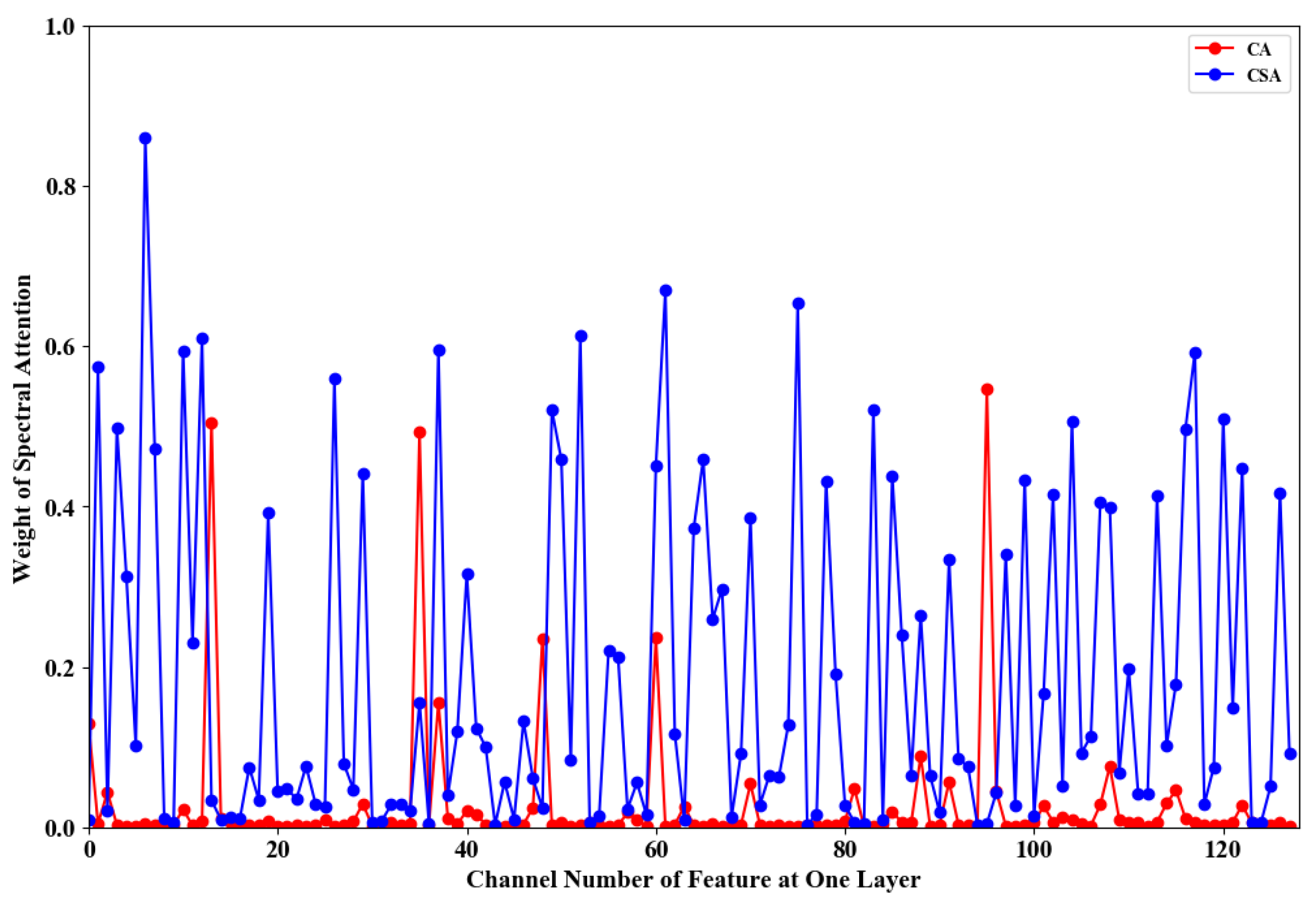
Although 2D GAP can calculate the specificity of the band, it pays far less attention to the channel than 3D GAP, as illustrated in Figure 7. While 3D GAP can better extract the five most crucial feature kernels, ignore the unnecessary features in Figure 7, which is accurate and efficient. Besides, from the outcome of CSA, it is clear that its higher weights distribute everywhere, which is viewed as not suitable for attention.
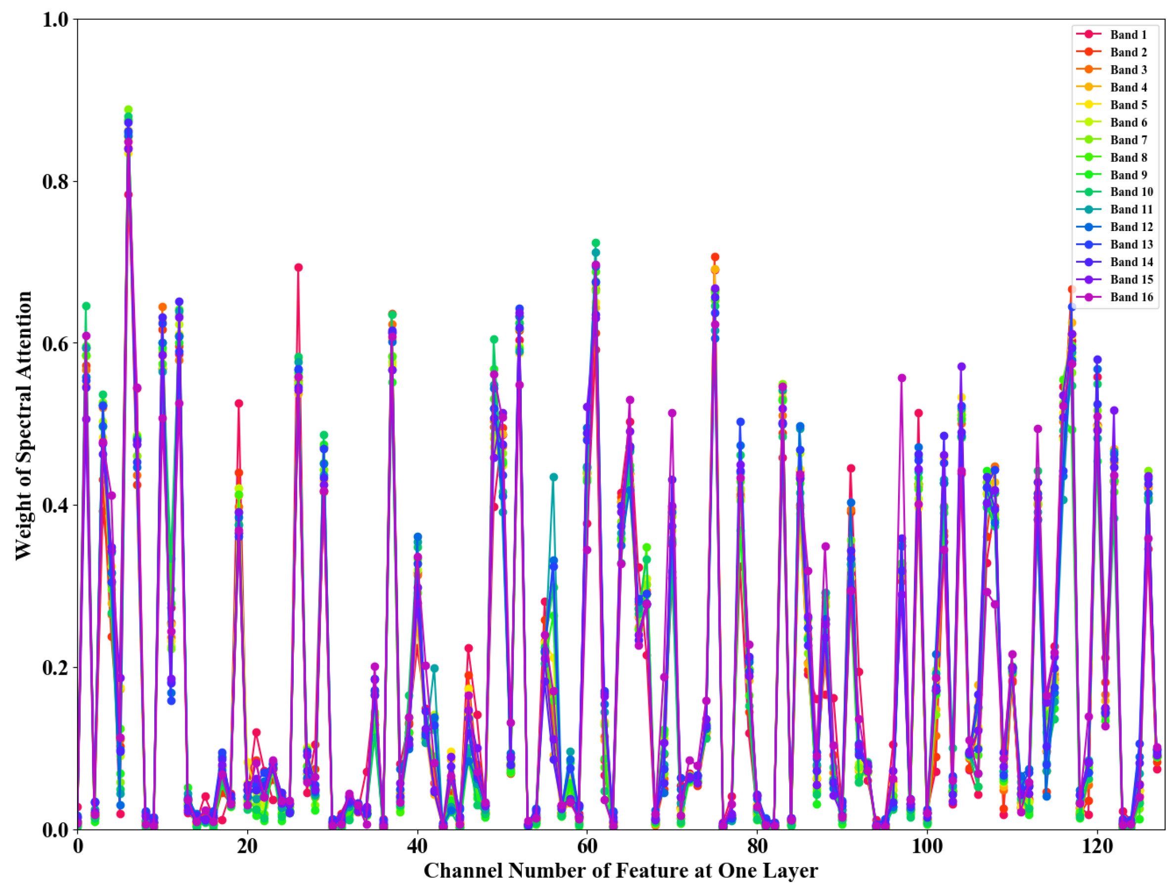
As shown in Figure 8, we can not only clearly see the dispersion of attention, but also the clustering in the figure reflects that the importance of most feature kernels is not changed by the change of band. In theory, 2D GAP can well avoid the limitations of 3D GAP in weight distribution and grasp the specificity of bands. However, if there is no a certain extent restriction, channel attention distribution will be dispersed and unbalanced with 2D GAP, and insignificant features will be extracted, which will hinder the improvement of the denoising ability of the model. This problem is that 2D GAP extracts local band information and pays more attention to the particularity of crawling bands. In contrast, the 3D GAP makes use of the global band information, so the former is difficult to accurately extract the effective features. The latter can be marvelous for grasping important noise reduction features.
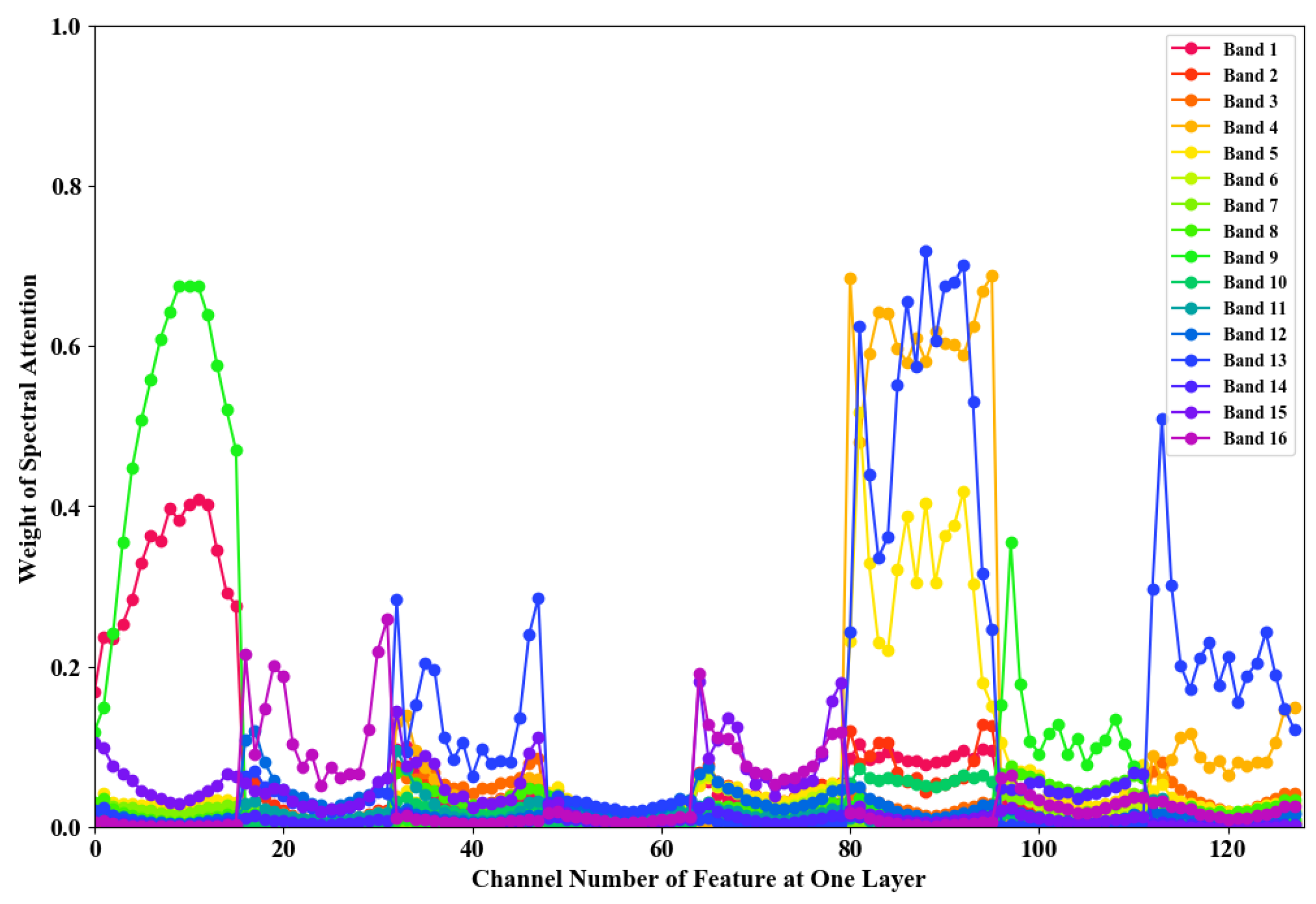
As shown in Figure 9, to capture band particularity by 2D GAP and avoid the defects, we exchange the dimensions of channel and band. After this, our neural network can not only comprehensively use all features extracted from local bands but also extract the importance of features. The more important features exist in the band, the more important the band can be well-reflected. 2D GAP after dimensional transformation can well focus on important bands and corresponding important features.
2.7. Loss Function
loss function is used for training proposed network, and it can be described as follows:
where represents the loss function of remote sensing HSIs. represents the result of SSCANet, represents the corresponding Ground-Truth in the dataset.
3. Result
3.1. Datasets
3.1.1. Synthetic Datasets
The lack of published remote sensing datasets is difficult to use directly for training. We are going to train with ICVL [59], a hyperspectral image dataset of natural scenery, and then use Pavia remote sensing dataset for transfer learning. In ICVL hyperspectral dataset [59], 201 images with a spatial resolution of are collected in 31 spectral bands (some sample images of ICVL are shown in Figure 10). Like QRNN3D [51], the training set consists of 100 images, 5 validation images, and the remaining images for testing. To extend the training set, we chopped a lot of overlapping volumes from the training HSIs and used each volume as a training sample. When a roll is planted, it has a spatial dimension of 64 by 64 and a spectral size of 31 to keep the whole spectrum of an HSI. Around 50,000 training samples are employed, and methods for enhancing the data, such as rotation and scaling, are also applied. In the test set, we used a rectangle to clip the center of each image.
In addition, we evaluated the sturdiness and adaptability of our model on hyperspectral datasets for remote sensing such as the Pavia Centre with 102 spectral bands and Pavia University with 103 spectral bands, both collected by the ROSIS sensor.
3.1.2. Real-World Datasets
In this section, we used real HSI Urban to validate our model. Urban collected data with a 210-band HYDICE hyperspectral system. It has been applied in practical HSI denoising experiments.
3.1.3. Metrics
To evaluate the performance of the above methods, we use five indicators widely used for HSI recovery, namely (I) Mean Peak signal-to-noise ratio (MPSNR), which is a classic cross-band average PSNR measure [60]; (ii) Mean Structural Similarity Index Measurement (MSSIM), based on The SSIM Measurement [60]; (iii) Mean Feature Similarity Index Measurement (MFSIM) introduced in [61]; (iv) Average ERGAS [62] and (v) average spectral angel mapper [63]. We use MPSNR and MSSIM in major papers.
3.2. Implementation Details
Prior to the training, we performed data enhancement, randomly clipped patches, and randomly flipped each image horizontally or vertically. The noise of the training dataset is set as non-i.i.d. and Mixture noise, the network hyperparameter Batch Size = 16, the initial Learning Rate = , and 50 epochs are iterated by cosine annealing algorithm [64]. All the DL-based methods are trained using Python 3.8.5, Pytorch 1.8.0, and an NVIDIA GPU GeForce GTX 3090 on the Ubuntu operating system.
Noise Setting
The most prevalent noise, i.e., Gaussian noise, impulse noise, deadline noise, and stripe noise [9,65,66], are typically present in real HSI. Using five different types of compound noise:
- Case 1: Non-i.i.d. Gaussian noise. Zero-mean Gaussian noise has distorted all bands with intensities ranging from 10 to 70.
- Case 2: Gaussian + Stripe noise. Non-i.i.d. Gaussian noise corrupts all bands as in Case 1. For the ICVL dataset, three out of ten bands are randomly selected to introduce stripe noise (5% to 15% percentages of columns).
- Case 3: Gaussian + Deadline noise. Except for the stripe noise being replaced by the deadline, the noise creation procedure is almost identical to Case 2.
- Case 4: Gaussian + Impulse noise. Each band is tainted by Gaussian noise, as in Case 1. Impulse noise with intensities ranging from 10% to 70% is randomly added to one-third of the bands.
- Case 5: Mixture noise. At least one of the noise types specified in Cases 1-4 corrupts each band at random.
3.3. Results of Synthetic Datasets
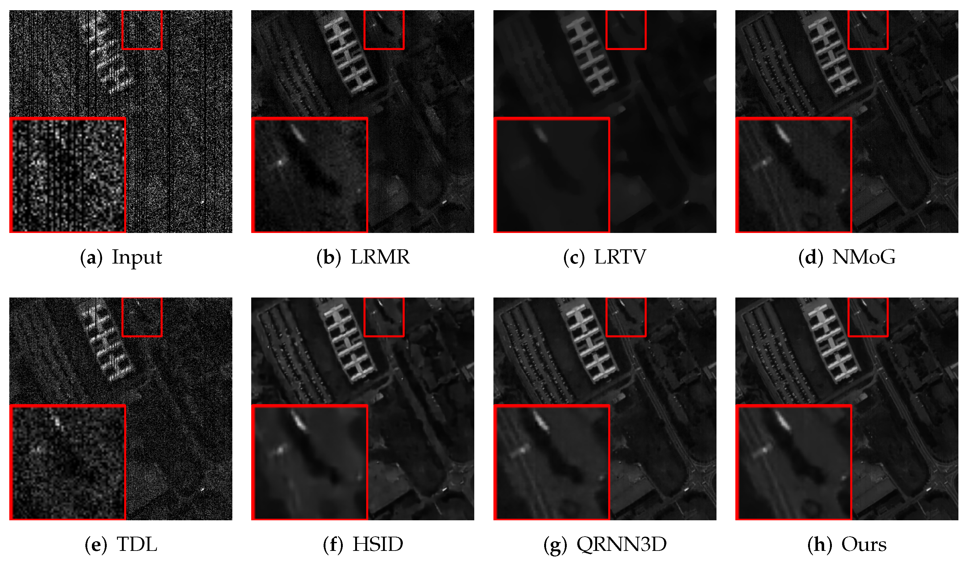
We contrasted six current SOTA denoising methods (namely LRMR [66], LRTV [67], NMoG [9], TDL [12], HSID [37] and QRNN3D [51]) with the proposed SSCANet on ICVL [59] composite images qualitatively or quantitatively, and Figure 11 and Table 1 display the outcomes, respectively:
Obviously, our visualization results have almost no residual noise compared to other approaches, and the PSNR and SSIM values are superior to those of different methods in the synthetic dataset ICVL.
To validate our method’s sturdiness using a simulated hyperspectral remote sensing dataset PaviaU, we also provide the visual results in Figure 12. While the other approaches still contain some visible noise, our method produces the most apparent outcome.
3.4. Results of Real Datasets
The quantitative outcomes are displayed in Figure 13 in this section, which compares these approaches using Urban datasets. We can observe that our approach also performs admirably for natural images.
As shown in Figure 13, our method is clearly superior to conventional approaches. And compared with the deep learning method, we are obviously superior to HSID in texture protection. The stripe noise at the bottom of the image is not removed by QRNN3D’s output, but our approach is more effective.
3.5. Ablation Study
Ablation studies on the proposed network’s components are presented to demonstrate the rationality of our network structure in this section.
First, the most basic U-Net based on 3D Conv is taken as the baseline. Then the SSCA block designed by us is added to strengthen the denoising effect of the network. Finally, the effect of using 2D Conv for the same structure is also verified in this part. For a fair comparison, these versions of networks are trained on the ICVL dataset for 30 epochs with mixture noise, and the quantitative outcomes are displayed in Table 2.
Effectiveness of the SCSA block. To analyze the impact of the SCSA block, which has the same structure as the SSCA block in our model, we describe ablation experiments. The only difference is that the dimension in the GAP process is . And we replace the SCSA basic block in SCSANet with a normal U-Net basic block, called UNet3D. Experimental data show that the basic block of the SCSA has been improved by 2.29 dB, which also indicates that it is important to design the network of structural spatio-spectral correlation and GCS for remote sensing characteristics.
Effectiveness of the SSCA block. We conducted ablation experiments to evaluate how the SSCA block affects our model, in which the dimension in the GAP process is . Experimental data shows that the SSCA block is 0.59 dB higher than the SCSA block.
Effectiveness of 3D Conv. To prove the contribution of the 3D Conv in our model, we conducted ablation experiments. We replace the 3D version of the SCA block with the 2D version, called the SCA2DNet. Experimental data shows that the 3D SCA block improves by 6.23 dB more than the 2D SCA block.
4. Discussion
Here, the suggested approach’s convergence and the features’ analysis will be covered. Please note that to keep this section’s discussion concise, we will use the ICVL dataset as our test example.
4.1. Convergence Analysis
To illustrate the implemented SSCANet’s convergence property, in Figure 14, we show the relationshipcurve between the quantity of training epochs and the value of the loss function defined in Section 2.7. This figure makes it clear that the suggested network can converge as the number of iterations rises.
4.2. Feature Analysis
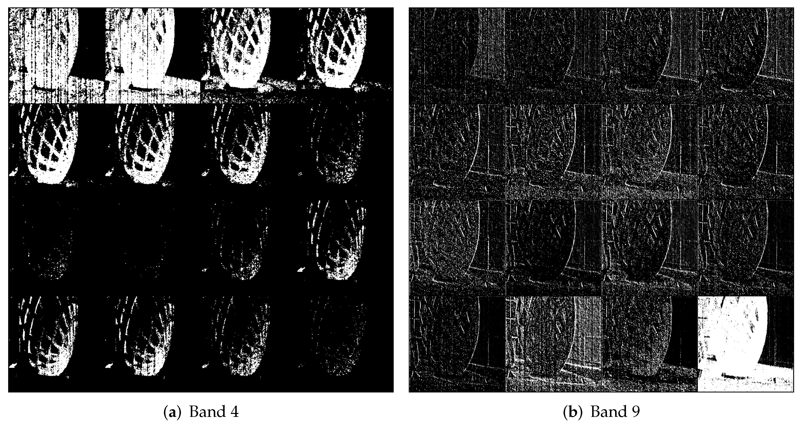
To illustrate the function of the proposed SSCANet more directly, we selected the feature map with the highest 16 weights in Band 9 and Band 4, respectively, according to the line chart in Figure 9. In addition, the feature map in Figure 15 is extracted by the SSCA block in the first encoding level of U-Net.
The analysis of the two figures mainly reflects three features of the SSCA block, as follows:
- Continuity of feature kernel extraction. In Figure 9, the serial numbers of feature kernels with high weight are continuous. The feature maps in Figure 15a,b also show similar feature extraction, respectively. Figure 15a mostly contains texture information, and Figure 15b mostly contains edge information.
- Selectivity of feature kernel extraction. SSCA block can select properties of different bands and extract corresponding features. For example, if there are many texture features in the current band, the weight of feature kernel related to texture will be considerable.
- Differences in feature kernel extraction. The feature kernel extracted by the SSCA block extracts a certain kind of similar features in a specific serial number intervals and different kinds of features in different serial number intervals. For example, the essential feature kernels in Figure 15a are concentrated in the range of , and the feature images are mostly different texture information; the vital feature kernels in Figure 15b are concentrated in the range of , and the feature maps are mostly different edge information.
5. Conclusions
Considering the importance of spatial-domain and spectral-domain to remote sensing HSI denoising, this paper designs an SSCANet based on U-Net network architecture. We apply 3D Conv to adapt to the diversity of band number of HSIs and extract spatial features and spectral features. In order to suppress the redundant information extracted by 3D Conv and strengthen the spatial and spectral domain features, we construct the SSCA block. This block begins by employing spatial attention to extract spatial information. Then we develop a spectral channel attention block to enhance the accuracy of attention, which can not only extract the specificity of the bands but also identify important noise bands and features. To ensure that the features recovered by upsampling are not coarse but rather more refined, we use U-Net with skip connections and a U-shaped structure to gather multi-scale information. Experimental results, both quantitative and qualitative, demonstrate that the SSCA block fully utilizes the spatial and spectral domain information, which greatly improves the image denoising effect, and both actual and synthetic datasets show noticeably better final outcomes.
In this work, the importance of different bands of the same feature kernel is almost the same, and only a small part of them differ greatly, but they have also been improved to some extent. For future work, if the importance of different B in the same feature kernels fluctuates greatly, the effect may be better in other domains.
Author Contributions
Conceptualization, H.-X.D.; formal analysis, H.-Z.S.; Methodology, X.-M.P.; project administration, C.W.; software, X.-M.P.; supervision, L.-J.D.; validation, X.-M.P.; visualization, X.-M.P.; writing—original draft, X.-M.P.; writing—review and editing, H.-Z.S. and L.-J.D. All authors have read and agreed to the published version of the manuscript.
Funding
This work is supported by the research start-up funding of Xihua University (RZ2000002862), and Basic Public Welfare Research in Zhejiang Province of China (LGG22F020036).
Institutional Review Board Statement
Not applicable.
Informed Consent Statement
Not applicable.
Data Availability Statement
The datasets generated during the study are available from the corresponding author on reasonable request.
Conflicts of Interest
The authors declare no conflict of interest.
Abbreviations
The following abbreviations are used in this manuscript:
| SSCA | Spatial and Spectral-Channel Attention |
| SCA | Spatial and Channel Attention |
| HSI | Hyperspectral Image |
| GAP | Global Average Pooling |
| DL | Deep Learning |
| 2D | 2-dimension |
| 3D | 3-dimension |
| Conv | convolution |
References
- Bourennane, S.; Fossati, C.; Cailly, A. Improvement of Classification for Hyperspectral Images Based on Tensor Modeling. IEEE Geosci. Remote Sens. Lett. 2010, 7, 801–805. [Google Scholar] [CrossRef]
- Li, Y.; Zhang, H.; Shen, Q. Spectral–Spatial Classification of Hyperspectral Imagery with 3D Convolutional Neural Network. Remote Sens. 2017, 9, 67. [Google Scholar] [CrossRef] [Green Version]
- Sun, W.; Tian, L.; Xu, Y.; Du, B.; Du, Q. A Randomized Subspace Learning Based Anomaly Detector for Hyperspectral Imagery. Remote Sens. 2018, 10, 417. [Google Scholar] [CrossRef] [Green Version]
- Xiong, F.; Zhou, J.; Qian, Y. Material Based Object Tracking in Hyperspectral Videos. IEEE Trans. Image Process. 2020, 29, 3719–3733. [Google Scholar] [CrossRef] [PubMed]
- Bioucas-Dias, J.M.; Plaza, A.; Dobigeon, N.; Parente, M.; Du, Q.; Gader, P.; Chanussot, J. Hyperspectral Unmixing Overview: Geometrical, Statistical, and Sparse Regression-Based Approaches. IEEE J. Sel. Top. Appl. Earth Obs. Remote Sens. 2012, 5, 354–379. [Google Scholar] [CrossRef] [Green Version]
- Huang, J.; Huang, T.Z.; Zhao, X.L.; Deng, L.J. Nonlocal Tensor-Based Sparse Hyperspectral Unmixing. IEEE Trans. Geosci. Remote Sens. 2021, 59, 6854–6868. [Google Scholar] [CrossRef]
- Rasti, B.; Chang, Y.; Dalsasso, E.; Denis, L.; Ghamisi, P. Image restoration for remote sensing: Overview and toolbox. arXiv 2021, arXiv:2107.00557. [Google Scholar] [CrossRef]
- Rasti, B.; Scheunders, P.; Ghamisi, P.; Licciardi, G.; Chanussot, J. Noise Reduction in Hyperspectral Imagery: Overview and Application. Remote Sens. 2018, 10, 482. [Google Scholar] [CrossRef] [Green Version]
- Chen, Y.; Cao, X.; Zhao, Q.; Meng, D.; Xu, Z. Denoising hyperspectral image with non-iid noise structure. IEEE Trans. Cybern. 2017, 48, 1054–1066. [Google Scholar] [CrossRef] [Green Version]
- Dabov, K.; Foi, A.; Katkovnik, V.; Egiazarian, K. Image denoising by sparse 3-D transform-domain collaborative filtering. IEEE Trans. Image Process. 2007, 16, 2080–2095. [Google Scholar] [CrossRef]
- Maggioni, M.; Katkovnik, V.; Egiazarian, K.; Foi, A. Nonlocal transform-domain filter for volumetric data denoising and reconstruction. IEEE Trans. Image Process. 2013, 22, 119–133. [Google Scholar] [CrossRef] [PubMed]
- Peng, Y.; Meng, D.; Xu, Z.; Gao, C.; Yang, Y.; Zhang, B. Decomposable nonlocal tensor dictionary learning for multispectral image denoising. In Proceedings of the IEEE Conference on Computer Vision and Pattern Recognition (CVPR), Columbus, OH, USA, 23–28 June 2014; pp. 2949–2956. [Google Scholar]
- Xie, Q.; Zhao, Q.; Meng, D.; Xu, Z.; Gu, S.; Zuo, W.; Zhang, L. Multispectral images denoising by intrinsic tensor sparsity regularization. In Proceedings of the IEEE Conference on Computer Vision and Pattern Recognition, Las Vegas, NV, USA, 27–30 June 2016; pp. 1692–1700. [Google Scholar]
- Chang, Y.; Yan, L.; Zhong, S. Hyper-laplacian regularized unidirectional low-rank tensor recovery for multispectral image denoising. In Proceedings of the IEEE Conference on Computer Vision and Pattern Recognition, Honolulu, HI, USA, 21–26 July 2017; pp. 4260–4268. [Google Scholar]
- Zhang, K.; Zuo, W.; Chen, Y.; Meng, D.; Zhang, L. Beyond a gaussian denoiser: Residual learning of deep cnn for image denoising. IEEE Trans. Image Process. 2017, 26, 3142–3155. [Google Scholar] [CrossRef] [PubMed] [Green Version]
- Ioffe, S.; Szegedy, C. Batch normalization: Accelerating deep network training by reducing internal covariate shift. In Proceedings of the International Conference on Machine Learning, PMLR, Lille, France, 7–9 July 2015; pp. 448–456. [Google Scholar]
- He, K.; Zhang, X.; Ren, S.; Sun, J. Deep residual learning for image recognition. In Proceedings of the IEEE Conference on Computer Vision and Pattern Recognition, Las Vegas, NV, USA, 27–30 June 2016; pp. 770–778. [Google Scholar]
- Ronneberger, O.; Fischer, P.; Brox, T. U-net: Convolutional networks for biomedical image segmentation. In Proceedings of the International Conference on Medical Image Computing and Computer-Assisted Intervention, Munich, Germany, 5–9 October 2015; Springer: New York, NY, USA, 2015; pp. 234–241. [Google Scholar]
- Woo, S.; Park, J.; Lee, J.Y.; Kweon, I.S. Cbam: Convolutional block attention module. In Proceedings of the European Conference on Computer Vision (ECCV), Munich, Germany, 8–14 September 2018; pp. 3–19. [Google Scholar]
- Vu, D.T.; Gonzalez, J.L.; Kim, M. Exploiting Global and Local Attentions for Heavy Rain Removal on Single Images. arXiv 2021, arXiv:2104.08126. [Google Scholar]
- Zhang, Z.; Ely, G.; Aeron, S.; Hao, N.; Kilmer, M. Novel Methods for Multilinear Data Completion and De-noising Based on Tensor-SVD. In Proceedings of the IEEE Conference on Computer Vision and Pattern Recognition (CVPR), Columbus, OH, USA, 23–28 June 2014. [Google Scholar]
- He, W.; Zhang, H.; Shen, H.; Zhang, L. Hyperspectral Image Denoising Using Local Low-Rank Matrix Recovery and Global Spatial–Spectral Total Variation. IEEE J. Sel. Top. Appl. Earth Obs. Remote Sens. 2018, 11, 713–729. [Google Scholar] [CrossRef]
- Zhuang, L.; Bioucas-Dias, J.M. Hyperspectral image denoising based on global and non-local low-rank factorizations. In Proceedings of the 2017 IEEE International Conference on Image Processing (ICIP), Beijing, China, 7–20 September 2017; pp. 1900–1904. [Google Scholar]
- Zhuang, L.; Bioucas-Dias, J.M. Fast hyperspectral image denoising and inpainting based on low-rank and sparse representations. IEEE J. Sel. Top. Appl. Earth Obs. Remote Sens. 2018, 11, 730–742. [Google Scholar] [CrossRef]
- Peng, C.; Chen, Y.; Kang, Z.; Chen, C.; Cheng, Q. Robust principal component analysis: A factorization-based approach with linear complexity. Inf. Sci. 2020, 513, 581–599. [Google Scholar] [CrossRef]
- Peng, C.; Liu, Y.; Chen, Y.; Wu, X.; Cheng, A.; Kang, Z.; Chen, C.; Cheng, Q. Hyperspectral Image Denoising Using Non-convex Local Low-rank and Sparse Separation with Spatial-Spectral Total Variation Regularization. arXiv 2022, arXiv:2201.02812. [Google Scholar]
- Maffei, A.; Haut, J.M.; Paoletti, M.E.; Plaza, J.; Bruzzone, L.; Plaza, A. A single model CNN for hyperspectral image denoising. IEEE Trans. Geosci. Remote Sens. 2019, 58, 2516–2529. [Google Scholar] [CrossRef]
- Zhang, Q.; Yuan, Q.; Li, J.; Liu, X.; Shen, H.; Zhang, L. Hybrid noise removal in hyperspectral imagery with a spatial–spectral gradient network. IEEE Trans. Geosci. Remote Sens. 2019, 57, 7317–7329. [Google Scholar] [CrossRef]
- Zhang, T.; Fu, Y.; Li, C. Hyperspectral Image Denoising with Realistic Data. In Proceedings of the IEEE/CVF International Conference on Computer Vision, Montreal, BC, Canada, 11–17 October 2021; pp. 2248–2257. [Google Scholar]
- Zhao, Y.; Zhai, D.; Jiang, J.; Liu, X. Adrn: Attention-based deep residual network for hyperspectral image denoising. In Proceedings of the ICASSP 2020—2020 IEEE International Conference on Acoustics, Speech and Signal Processing (ICASSP), Barcelona, Spain, 4–8 May 2020; pp. 2668–2672. [Google Scholar]
- Buades, A.; Coll, B.; Morel, J.M. A non-local algorithm for image denoising. In Proceedings of the 2005 IEEE Computer Society Conference on Computer Vision and Pattern Recognition (CVPR’05), San Diego, CA, USA, 20–26 June 2005; Volume 2, pp. 60–65. [Google Scholar] [CrossRef]
- Zhao, Y.Q.; Yang, J. Hyperspectral Image Denoising via Sparse Representation and Low-Rank Constraint. IEEE Trans. Geosci. Remote Sens. 2015, 53, 296–308. [Google Scholar] [CrossRef]
- Liu, S.; Jiao, L.; Yang, S. Hierarchical Sparse Learning with Spectral-Spatial Information for Hyperspectral Imagery Denoising. Sensors 2016, 16, 1718. [Google Scholar] [CrossRef] [PubMed] [Green Version]
- Song, X.; Wu, L.; Hao, H.; Xu, W. Hyperspectral Image Denoising Based on Spectral Dictionary Learning and Sparse Coding. Electronics 2019, 8, 86. [Google Scholar] [CrossRef] [Green Version]
- Xue, T.; Wang, Y.; Chen, Y.; Jia, J.; Wen, M.; Guo, R.; Wu, T.; Deng, X. Mixed Noise Estimation Model for Optimized Kernel Minimum Noise Fraction Transformation in Hyperspectral Image Dimensionality Reduction. Remote Sens. 2021, 13, 2607. [Google Scholar] [CrossRef]
- Chang, Y.; Yan, L.; Fang, H.; Zhong, S.; Liao, W. HSI-DeNet: Hyperspectral image restoration via convolutional neural network. IEEE Trans. Geosci. Remote Sens. 2018, 57, 667–682. [Google Scholar] [CrossRef]
- Yuan, Q.; Zhang, Q.; Li, J.; Shen, H.; Zhang, L. Hyperspectral image denoising employing a spatial—Spectral deep residual convolutional neural network. IEEE Trans. Geosci. Remote Sens. 2018, 57, 1205–1218. [Google Scholar] [CrossRef] [Green Version]
- Wang, C.; Zhang, L.; Wei, W.; Zhang, Y. When Low Rank Representation Based Hyperspectral Imagery Classification Meets Segmented Stacked Denoising Auto-Encoder Based Spatial-Spectral Feature. Remote Sens. 2018, 10, 284. [Google Scholar] [CrossRef] [Green Version]
- Fu, X.; Wang, W.; Huang, Y.; Ding, X.; Paisley, J. Deep Multiscale Detail Networks for Multiband Spectral Image Sharpening. IEEE Trans. Neural Netw. Learn. Syst. 2020, 32, 2090–2104. [Google Scholar] [CrossRef]
- Yang, J.; Fu, X.; Hu, Y.; Huang, Y.; Ding, X.; Paisley, J. PanNet: A Deep Network Architecture for Pan-Sharpening. In Proceedings of the 2017 IEEE International Conference on Computer Vision (ICCV), 2017, Venice, Italy, 22–29 October 2017; pp. 1753–1761. [Google Scholar] [CrossRef]
- Zhuang, P.; Liu, Q.; Ding, X. Pan-GGF: A probabilistic method for pan-sharpening with gradient domain guided image filtering. Signal Process. 2019, 156, 177–190. [Google Scholar] [CrossRef]
- Guo, P.; Zhuang, P.; Guo, Y. Bayesian Pan-Sharpening with Multiorder Gradient-Based Deep Network Constraints. IEEE J. Sel. Top. Appl. Earth Obs. Remote Sens. 2020, 13, 950–962. [Google Scholar] [CrossRef]
- Yang, Y.; Lu, H.; Huang, S.; Tu, W. Pansharpening Based on Joint-Guided Detail Extraction. IEEE J. Sel. Top. Appl. Earth Obs. Remote Sens. 2021, 14, 389–401. [Google Scholar] [CrossRef]
- Yang, Y.; Wu, L.; Huang, S.; Wan, W.; Tu, W.; Lu, H. Multiband Remote Sensing Image Pansharpening Based on Dual-Injection Model. IEEE J. Sel. Top. Appl. Earth Obs. Remote Sens. 2020, 13, 1888–1904. [Google Scholar] [CrossRef]
- Cao, X.; Yao, J.; Xu, Z.; Meng, D. Hyperspectral Image Classification with Convolutional Neural Network and Active Learning. IEEE Trans. Geosci. Remote Sens. 2020, 58, 4604–4616. [Google Scholar] [CrossRef]
- Cao, X.; Fu, X.; Xu, C.; Meng, D. Deep Spatial-Spectral Global Reasoning Network for Hyperspectral Image Denoising. IEEE Trans. Geosci. Remote Sens. 2021, 60, 1–14. [Google Scholar] [CrossRef]
- Dian, R.; Li, S.; Guo, A.; Fang, L. Deep hyperspectral image sharpening. IEEE Trans. Neural Netw. Learn. Syst. 2018, 29, 5345–5355. [Google Scholar] [CrossRef] [PubMed]
- Dian, R.; Li, S.; Fang, L. Learning a low tensor-train rank representation for hyperspectral image super-resolution. IEEE Trans. Neural Netw. Learn. Syst. 2019, 30, 2672–2683. [Google Scholar] [CrossRef] [PubMed]
- Hong, D.; Gao, L.; Yokoya, N.; Yao, J.; Chanussot, J.; Du, Q.; Zhang, B. More Diverse Means Better: Multimodal Deep Learning Meets Remote-Sensing Imagery Classification. IEEE Trans. Geosci. Remote Sens. 2021, 59, 4340–4354. [Google Scholar] [CrossRef]
- Zhang, T.J.; Deng, L.J.; Huang, T.Z.; Chanussot, J.; Vivone, G. A Triple-Double Convolutional Neural Network for Panchromatic Sharpening. IEEE Trans. Neural Netw. Learn. Syst. 2022. [Google Scholar] [CrossRef]
- Wei, K.; Fu, Y.; Huang, H. 3-D Quasi-Recurrent Neural Network for Hyperspectral Image Denoising. IEEE Trans. Neural Netw. Learn. Syst. 2020, 32, 363–375. [Google Scholar] [CrossRef] [Green Version]
- Aggarwal, H.K.; Majumdar, A. Mixed Gaussian and impulse denoising of hyperspectral images. In Proceedings of the 2015 IEEE International Geoscience and Remote Sensing Symposium (IGARSS), Milan, Italy, 26–31 July 2015; pp. 429–432. [Google Scholar]
- Dong, W.; Wang, P.; Yin, W.; Shi, G.; Wu, F.; Lu, X. Denoising prior driven deep neural network for image restoration. IEEE Trans. Pattern Anal. Mach. Intell. 2018, 41, 2305–2318. [Google Scholar] [CrossRef] [Green Version]
- Li, G.; He, X.; Zhang, W.; Chang, H.; Dong, L.; Lin, L. Non-locally enhanced encoder-decoder network for single image de-raining. In Proceedings of the 26th ACM international conference on Multimedia, Seoul, Korea, 22–26 October 2018; pp. 1056–1064. [Google Scholar]
- Jin, Z.R.; Zhang, T.J.; Jiang, T.X.; Vivone, G.; Deng, L.J. LAGConv: Local-context Adaptive Convolution Kernels with Global Harmonic Bias for Pansharpening. In Proceedings of the AAAI Conference on Artificial Intelligence (AAAI), Virtual, 22 February–1 March 2022. [Google Scholar]
- Hu, J.F.; Huang, T.Z.; Deng, L.J.; Jiang, T.X.; Vivone, G.; Chanussot, J. Hyperspectral Image Super-Resolution via Deep Spatiospectral Attention Convolutional Neural Networks. IEEE Trans. Neural Netw. Learn. Syst. 2021. [Google Scholar] [CrossRef]
- Ni, J.; Wu, J.; Tong, J.; Wei, M.; Chen, Z. SSCA-Net: Simultaneous Self-and Channel-Attention Neural Network for Multiscale Structure-Preserving Vessel Segmentation. BioMed Res. Int. 2020, 2021, 6622253. [Google Scholar] [CrossRef]
- Wu, X.; Huang, T.Z.; Deng, L.J.; Zhang, T.J. Dynamic Cross Feature Fusion for Remote Sensing Pansharpening. In Proceedings of the IEEE/CVF International Conference on Computer Vision (ICCV), Montreal, BC, Canada, 11–17 October 2021; pp. 14687–14696. [Google Scholar]
- Arad, B.; Ben-Shahar, O. Sparse recovery of hyperspectral signal from natural RGB images. In Proceedings of the European Conference on Computer Vision, Amsterdam, The Netherlands, 11–14 October 2016; Springer: New York, NY, USA, 2016; pp. 19–34. [Google Scholar]
- Wang, Z.; Bovik, A.C.; Sheikh, H.R.; Simoncelli, E.P. Image quality assessment: From error visibility to structural similarity. IEEE Trans. Image Process. 2004, 13, 600–612. [Google Scholar] [CrossRef] [PubMed] [Green Version]
- Zhang, L.; Zhang, L.; Mou, X.; Zhang, D. FSIM: A feature similarity index for image quality assessment. IEEE Trans. Image Process. 2011, 20, 2378–2386. [Google Scholar] [CrossRef] [Green Version]
- Wald, L. Quality of high resolution synthesised images: Is there a simple criterion? In Proceedings of the Third Conference “Fusion of Earth Data: Merging Point Measurements, Raster Maps and Remotely Sensed Images”, SEE/URISCA, Sophia Antipolis, France, 26–28 January 2000; pp. 99–103. [Google Scholar]
- Yuhas, R.H.; Goetz, A.F.; Boardman, J.W. Discrimination among semi-arid landscape endmembers using the spectral angle mapper (SAM) algorithm. In Proceedings of the n JPL, Summaries of the Third Annual JPL Airborne Geoscience Workshop, California, CA, USA, 1–5 June 1992; Volume 1, pp. 147–149. [Google Scholar]
- Loshchilov, I.; Hutter, F. Sgdr: Stochastic gradient descent with warm restarts. arXiv 2016, arXiv:1608.03983. [Google Scholar]
- He, K.; Zhang, X.; Ren, S.; Sun, J. Delving deep into rectifiers: Surpassing human-level performance on imagenet classification. In Proceedings of the IEEE International Conference on Computer Vision, Santiago, Chile, 7–13 December 2015; pp. 1026–1034. [Google Scholar]
- Zhang, H.; He, W.; Zhang, L.; Shen, H.; Yuan, Q. Hyperspectral image restoration using low-rank matrix recovery. IEEE Trans. Geosci. Remote Sens. 2014, 52, 4729–4743. [Google Scholar] [CrossRef]
- He, W.; Zhang, H.; Zhang, L.; Shen, H. Total-variation-regularized low-rank matrix factorization for hyperspectral image restoration. IEEE Trans. Geosci. Remote Sens. 2016, 54, 178–188. [Google Scholar] [CrossRef]
Figure 1.
An evaluation between our algorithm and the state-of-the-art NMoG denoising method [9].
Figure 1.
An evaluation between our algorithm and the state-of-the-art NMoG denoising method [9].

Figure 2.
Architecture of our model SSCANet. The digit below the block indicates the block’s matching output channels.
Figure 2.
Architecture of our model SSCANet. The digit below the block indicates the block’s matching output channels.

Figure 3.
2D and 3D Conv schematics. H, W, B represent image height, image width, and image band, respectively. In 2D Conv, the kernel number must manually adapt to the band number of the input HSI. 3D Conv can auto-adapt to bands of HSI and simultaneously extract spatial-domain and spectral-domain information.

Figure 4.
An illustration of the SSCA block, which mainly includes two attentions, i.e., spatial attention (SA) in blue area and spectral attention in yellow area. For the latter spectral attention, we build three versions (see more details from Figure 5) and finally select the SCA with the best performance as the module.

Figure 5.
The three different versions of the spectral attention, i.e., CA block, CSA block and SCA block. We finally select the SCA with the best performance as the module of SSCA block.
Figure 5.
The three different versions of the spectral attention, i.e., CA block, CSA block and SCA block. We finally select the SCA with the best performance as the module of SSCA block.

Figure 6.
The bar chart of kernel weight divergence between different bands of CSA and SCA. The horizontal axis Weight Divergence indicates , and the vertical axis Number indicates the number of weight divergence.
Figure 6.
The bar chart of kernel weight divergence between different bands of CSA and SCA. The horizontal axis Weight Divergence indicates , and the vertical axis Number indicates the number of weight divergence.

Figure 7.
The line chart of kernel weight distribution of CA and CSA. The horizontal axis “Channel Number of Feature at One Layer” is also equal to the number of feature kernels, and the vertical axis “Weight of Spectral Attention” indicates the weight learned from spectral attention. In addition, the five highest in the CA red line are considered to be the five most important feature kernels. And the weight of CSA blue line is calculated by the mean of each band. From the outcome of CSA, it is clear that its high weights distribute everywhere, which is viewed as being not good for attention.

Figure 8.
The line chart of kernel weight learned by CSA. The dimension of the feature kernel obtained by 3D Conv is , so the quantity of bands can be changed by the feature kernel of the network, which is not necessarily equal to the number of bands in the HSI. CSA that only uses 2D GAP is more flexible in weight allocation, but its line chart is very confused due to its lack of concentration (i.e., distribute everywhere). It is not as good as the SCA line chart to clearly see important bands and the corresponding interval of important feature channel numbers.

Figure 9.
The line chart of kernel weight learned by SCA. The network extracts the four most important bands, i.e., band 1, band 4, band 5, and band 9. The high weights of band 9 and band 4 are concentrated between [0, 20] and [80, 100], respectively, indicating that the attention of the network is relatively concentrated. Feature maps (see more details in Section 4.2) also show that the feature types in the connected interval are similar.

Figure 10.
This is the ICVL Dataset.

Figure 11.
Qualitative comparison of the six denoising methods on the ICVL dataset, where the first column is noisy HSI, and the last column is the corresponding GT.
Figure 11.
Qualitative comparison of the six denoising methods on the ICVL dataset, where the first column is noisy HSI, and the last column is the corresponding GT.

Figure 12.
Visual results of competing denoising methods on Pavia University dataset.

Figure 13.
A comparison of our method using the Urban real dataset.

Figure 14.
The convergence curve of the proposed SSCANet.

Figure 15.
16 important feature maps in the Band 4 and 9.


Table 1.
Quantitative results of different methods in five complex noise cases on ICVL dataset. Best and second best scores are highlighted and underlined.
Table 1.
Quantitative results of different methods in five complex noise cases on ICVL dataset. Best and second best scores are highlighted and underlined.
| Noisy HSI | LRMR [66] | LRTV [67] | NMoG [9] | TDL [12] | HSID [37] | QRNN3D [51] | Ours | |
|---|---|---|---|---|---|---|---|---|
| Case 1: Non-i.i.d. Gaussian | ||||||||
| PSNR | 18.25 | 32.80 | 33.62 | 34.51 | 28.55 | 38.63 | 41.75 | 43.44 |
| SSIM | 0.168 | 0.719 | 0.905 | 0.812 | 0.470 | 0.981 | 0.989 | 0.993 |
| Case 2: Gaussian + Stripe | ||||||||
| PSNR | 17.80 | 32.62 | 33.49 | 33.87 | 34.60 | 38.34 | 41.49 | 43.25 |
| SSIM | 0.159 | 0.717 | 0.905 | 0.799 | 0.807 | 0.981 | 0.988 | 0.992 |
| Case 3: Gaussian + Deadline | ||||||||
| PSNR | 17.61 | 31.83 | 32.37 | 32.87 | 34.26 | 37.81 | 41.47 | 43.42 |
| SSIM | 0.155 | 0.709 | 0.895 | 0.797 | 0.821 | 0.980 | 0.988 | 0.993 |
| Case 4: Gaussian + Impulse | ||||||||
| PSNR | 14.80 | 29.70 | 31.56 | 28.60 | 28.69 | 35.95 | 39.60 | 40.99 |
| SSIM | 0.114 | 0.623 | 0.871 | 0.652 | 0.624 | 0.966 | 0.975 | 0.978 |
| Case 5: Mixture | ||||||||
| PSNR | 14.08 | 28.68 | 30.47 | 27.31 | 27.43 | 34.43 | 38.63 | 40.28 |
| SSIM | 0.099 | 0.608 | 0.858 | 0.632 | 0.604 | 0.964 | 0.973 | 0.978 |
Table 2.
Analysis of the impact of the suggested network architecture. Best and second best scores are highlighted and underlined.
Table 2.
Analysis of the impact of the suggested network architecture. Best and second best scores are highlighted and underlined.
| SCSA | SCA | SSCA | 3D | PSNR | SSIM | |
|---|---|---|---|---|---|---|
| UNet3D | ✓ | 37.13 | 0.968 | |||
| SCSANet | ✓ | ✓ | 39.42 | 0.975 | ||
| SCANet | ✓ | ✓ | 39.82 | 0.978 | ||
| SSCANet | ✓ | ✓ | 40.01 | 0.978 | ||
| SCA2DNet | ✓ | 33.59 | 0.948 |
Publisher’s Note: MDPI stays neutral with regard to jurisdictional claims in published maps and institutional affiliations. |
© 2022 by the authors. Licensee MDPI, Basel, Switzerland. This article is an open access article distributed under the terms and conditions of the Creative Commons Attribution (CC BY) license (https://creativecommons.org/licenses/by/4.0/).
Share and Cite
MDPI and ACS Style
Dou, H.-X.; Pan, X.-M.; Wang, C.; Shen, H.-Z.; Deng, L.-J. Spatial and Spectral-Channel Attention Network for Denoising on Hyperspectral Remote Sensing Image. Remote Sens. 2022, 14, 3338. https://0-doi-org.brum.beds.ac.uk/10.3390/rs14143338
AMA Style
Dou H-X, Pan X-M, Wang C, Shen H-Z, Deng L-J. Spatial and Spectral-Channel Attention Network for Denoising on Hyperspectral Remote Sensing Image. Remote Sensing. 2022; 14(14):3338. https://0-doi-org.brum.beds.ac.uk/10.3390/rs14143338
Chicago/Turabian StyleDou, Hong-Xia, Xiao-Miao Pan, Chao Wang, Hao-Zhen Shen, and Liang-Jian Deng. 2022. "Spatial and Spectral-Channel Attention Network for Denoising on Hyperspectral Remote Sensing Image" Remote Sensing 14, no. 14: 3338. https://0-doi-org.brum.beds.ac.uk/10.3390/rs14143338
Note that from the first issue of 2016, this journal uses article numbers instead of page numbers. See further details here.