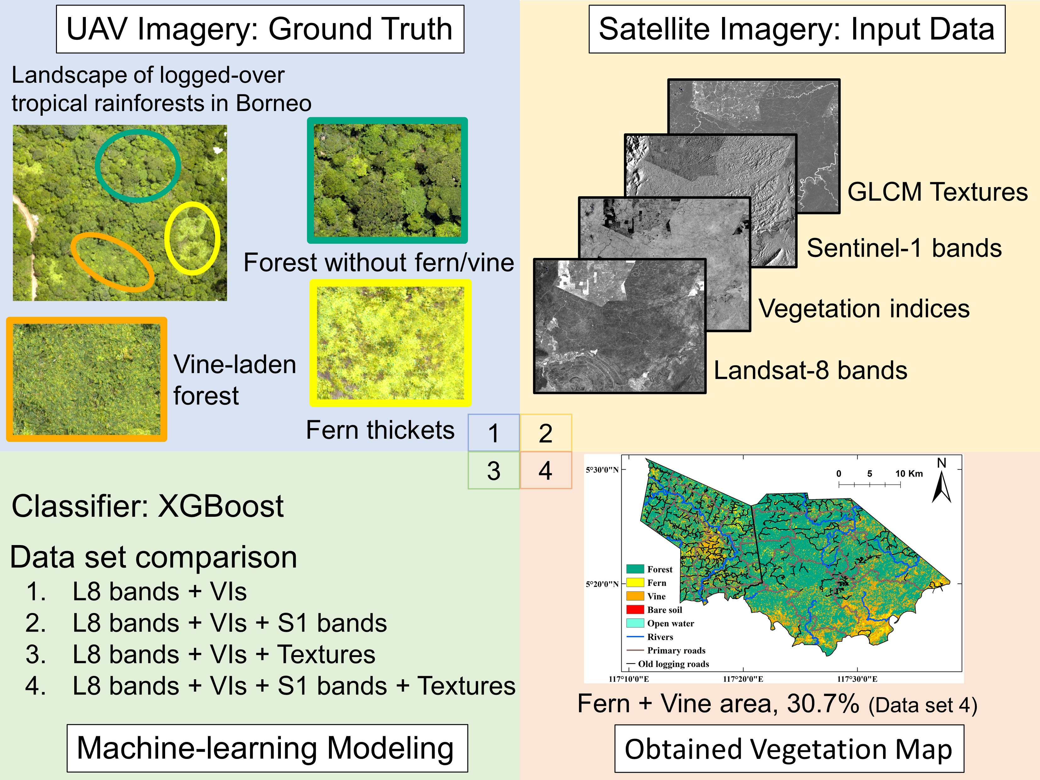
Mapping the Spatial Distribution of Fern Thickets and Vine-Laden Forests in the Landscape of Bornean Logged-Over Tropical Secondary Rainforests

Abstract

Forest degradation has been most frequently defined as an anthropogenic reduction in biomass compared with reference biomass in extant forests. However, so-defined “degraded forests” may widely vary in terms of recoverability. A prolonged loss of recoverability, commonly described as a loss of resilience, poses a true threat to global environments. In Bornean logged-over forests, dense thickets of ferns and vines have been observed to cause arrested secondary succession, and their area may indicate the extent of slow biomass recovery. Therefore, we aimed to discriminate the fern thickets and vine-laden forests from those logged-over forests without dense ferns and vines, as well as mapping their distributions, with the aid of Landsat-8 satellite imagery and machine learning modeling. During the process, we tested whether the gray-level co-occurrence matrix (GLCM) textures of Landsat data and Sentinel-1 C-band SAR data were helpful for this classification. Our study sites were Deramakot and Tangkulap Forest Reserves—commercial production forests in Sabah, Malaysian Borneo. First, we flew drones and obtained aerial images that were used as ground truth for the supervised classification. Subsequently, a machine-learning model with a gradient-boosting decision tree was iteratively tested in order to derive the best model for the classification of the vegetation. Finally, the best model was extrapolated to the entire forest reserve and used to map three classes of vegetation (fern thickets, vine-laden forests, and logged-over forests without ferns and vines) and two non-vegetation classes (bare soil and open water). The overall classification accuracy of the best model was 86.6%; however, by combining the fern and vine classes into the same category, the accuracy was improved to 91.5%. The GLCM texture variables were especially effective at separating fern/vine vegetation from the non-degraded forest, but the SAR data showed a limited effect. Our final vegetation map showed that 30.7% of the reserves were occupied by ferns or vines, which may lead to arrested succession. Considering that our study site was once certified as a well-managed forest, the area of degraded forests with a high risk of loss of resilience is expected to be much broader in other Bornean production forests.

1. Introduction

Tropical forests play an important role in providing ecosystem services, such as carbon sequestration and biodiversity conservation [1,2,3]; however, the provision of ecosystem services is highly threatened by forest degradation. One of the most widely used definitions of forest degradation is related to the decline of above-ground biomass (AGB) derived from human activity, sensu IPCC’s [4]. According to such definitions, extant forests with anthropogenically reduced biomass compared with reference biomass are defined as “degraded forests”. However, so-defined “degraded forests” may widely vary in terms of recoverability; some forests recover steadily, while others may not. A prolonged loss of recoverability, commonly described as the loss of resilience, poses true threats to the global environment, as it entails the perpetuated loss of carbon stock and biodiversity. Therefore, it is necessary to evaluate forest degradation in terms of recoverability, and to identify where interventions are needed to enhance resilience.

Recent plot-scale (e.g., 1–100 ha) studies have revealed that the recoverability of tropical forests after anthropogenic disturbance varies greatly, depending on the past land-use [5], edaphic conditions [6], seed dispersal limitations [7], climate [8], and invasion of herbaceous plants or woody vines [9,10,11,12]. Considering that a landscape consists of a matrix of vegetation patches with variable recoverability, landscape-level assessment should be necessary. There are, however, a few studies that have evaluated the recoverability of tropical forests at the landscape scale [13] because it is difficult to directly evaluate or predict the recoverability based on physical vegetation attributes on the ground.

In this study, we focused on ferns or vines as an indicator of forest degradation, which may pose a risk of slow biomass recovery. In Borneo, commercial selective logging has been repeated in a short-term for timber production, and it has been observed that the patches which experienced harsh logging did not recover for decades [14]. Remnant stands are often covered by dense ferns (e.g., Dicranopteris spp.) or vine thickets (e.g., lianas such as Uncaria spp. or climbing bamboo Dinochloa spp. [10,15]; Figure 1c). Previous studies of other regions have suggested that the invasion of ferns or vines can arrest the early phase of the succession and retard tropical forest recovery by competing against the remanent trees and recruited seedlings in the Neotropics [9], Afro-tropical [16], and other regions in Asia [10,12,17]. This has also been observed in the logged-over secondary forest in Borneo: the coverage of ferns or vines retarded the AGB recovery by changing forest dynamic processes, reducing the growth, survival, and recruitment of the remanent trees ([18]; Takeshige unpublished data). Due to their strong negative effect on recovery, the presence of ferns or vines can be used as an indicator of forest degradation with retarded biomass recovery.

The vine distribution in tropical forests has been examined through the use of hyper-spectral data combined with an airborne platform [19,20,21]. These techniques may be rather limited, in terms of applicability, due to their high cost and limited availability. To overcome this problem, optical satellite data which are open to the public, such as Landsat or Sentinel series imageries, can be used instead. Matongera et al. [22] have demonstrated the possibility of mapping the distribution of bracken fern (Pteridium spp.) thickets by using Landsat 8 imagery, and Chandler et al. [23] have mapped the vine-laden forest by using the Sentinel-2 imagery of Bornean tropical rainforests. However, no study has classified both vegetation types, which together threaten forest recovery, within the same landscape. Fern thickets and vine-laden stands often form a continuum of vegetation. Therefore, we tested whether fern thickets and vine-laden forests can be discriminated from each other within the same landscape using optical satellite data.

The wavelength regions that are important for distinguishing ferns or vines from trees have been reported variously. For canopy-level separation between vines and trees in tropical forests, detailed studies using hyperspectral spectroscopy have been conducted and two wavelength regions have been reported to be important [24]: the visible green region, which represents the characteristics of chlorophyll and carotenoid concentration [21,25,26,27], and the shortwave infrared (SWIR) region, which represents water content [26,27]. When using a multispectral optical satellite sensor, the visible green region of Sentinel-2 is especially helpful [23]. Ferns represent more distinct spectral characteristics from trees than vines do, and the visible green [28] and near-infrared (NIR) wavelength regions [29,30,31] have been shown to be useful for separating bracken ferns from trees in multispectral satellite imagery. In addition to the surface reflectance, vegetation indices have been used to enhance the optical properties of the ferns or vines [22,23,28]. For vegetation classification, besides vegetation indices, information of the gray-level co-occurrence matrix (GLCM) texture measures [32] and synthetic aperture radar (SAR) have also been commonly used to improve the classification accuracy [33,34,35,36]; however, no studies have applied either GLCM textures or SAR data to classify fern thickets or vine-laden forests.

In this study, we aimed to map the spatial distribution of the degraded forests, indicated by fern or vine coverage, by using remote sensing techniques on medium-resolution satellite imagery and machine learning modeling. The best machine learning classifier model obtained was spatially extrapolated and used to map the vegetation, in order to show the distribution of fern thickets and vine-laden forests. During the process, we compared which of the following variables were particularly useful for separating fern thickets and/or vines from trees: the surface reflectance of Landsat-8, vegetation indices, GLCM texture measures, and Sentinel-1 C-band SAR data.

2. Materials and Methods

2.1. Study Site

This study was conducted in two adjacent forest reserves in Sabah, Malaysian Borneo: Deramakot (5°14′–28′N, 117°20′–38′E, 55,083 ha) and Tangkulap Forest Reserve (5°18′–31′N, 117°11′–22′E, 27,550 ha) (Figure 1a). The climate of this region is humid equatorial. The mean annual temperature of this area is 25–27 °C and the mean annual precipitation is 2300–3000 mm, with slight seasonal variations. The altitude in the large parts of the reserves ranges between 20–300 m above sea level. Nearly the entire area of the forest reserves was originally covered with lowland dipterocarp forests [37].

The logging history of the two forest reserves differs [38]. Deramakot and Tangkulap were initially logged in 1956 and the 1970s, respectively, and conventional logging was carried out there. In 1989, the logging activities of Deramakot were suspended for regrowth. Then, a long-term management plan with reduced-impact logging was introduced in 1995. In 1997, Deramakot was certified as “well-managed” by an international certification body, the Forest Stewardship Council (FSC), for the first time regarding tropical natural forests [39]. On the other hand, Tangkulap was repeatedly logged using conventional techniques until 2002, after which all logging activities were suspended for regrowth. Previous studies have reported that much heavier logging was conducted over greater areas in Tangkulap, compared with Deramakot, in the 1990s [40,41].

As a result of the past logging activities, the forests in the reserves are in various stages of development, from well-developed forest patches, pioneer tree species-dominated patches, to highly degraded forest patches with ferns and/or vines ([14,42], as seen in Figure 1c). The fern thickets are mainly composed of pure colonies of Dicranopteris linearis, one of the most common ferns in the wetter parts of tropical and sub-tropical regions in the Old World [43]. These thickets were mainly observed in the open canopy forest with low AGB. The vine-laden forests are composed of trees with lianas (e.g., Uncaria spp.) or climbing bamboo (e.g., Dinochloa spp.), accompanied by herbaceous plants such as Scleria spp., Rubus spp., or Etlingera spp. (wild ginger). When compared to forests with fern thickets, vine-laden forests tend to present a wider range of AGB, from relatively developed forests to open-canopy forests. In particular, in an open-canopy forest, fern thickets and vine-laden stands often form a continuum of vegetation.

2.2. Mapping Procedure

Mapping consisted of three parts; the workflow is shown in Figure 2. First, we obtained photographs using drones, which were used as supervised data for the subsequent mapping. Second, we pre-processed satellite imagery and calculated some variables for constructing a classification model. Finally, we trained the machine learning vegetation classification model and obtained the objective vegetation map by extrapolating the tuned classification model to the satellite imagery.

2.2.1. UAV Imagery Processing

We flew unmanned aerial vehicles (UAVs; Mavic 2 Pro and Phantom4 Pro, DJI) and obtained aerial photography in August and September 2019 as ground-truth vegetation data. We took pictures of the 18 plots of Kitayama et al. [44], 11 plots of Langner et al. [45], two plots of Imai et al. [46], and some of the abandoned logging roads (see Figure 1b). The total flight area was about 820 ha. We used the UgCS PRO v3.3 software (SPH Engineering, Latvia) as the operational software for the UAV. For each flight, we set various flight parameters. For the flights over the plots, we set forward overlap as 90%, side overlap as 80%, and flight height as 100 m from the ground, as indicated by the digital elevation model of the Shuttle Radar Topography Mission (SRTM). For the flights over the abandoned logging roads, we set forward overlap as 80%, side overlap as 70%, and flight height as 120 m from the ground.

From the aerial pictures, we constructed orthomosaic photos using the SfM software, Metashape Professional v1.53 (Agisoft, Russia). We extracted forests without ferns or vines, fern thickets, vine-laden forests, bare soil, and open water by visual inspection from the orthomosaic photos using Arc Map v10.6.1 (ESRI, U.S.). The extracted shapes were grid-segmented along with the Landsat pixels, and the area of each class within a grid was calculated. Only grids with 33% or greater coverage of a given class (i.e., 0.30 ha) were selected as supervised data for the classification model. As a result, we obtained 1242 grid segments, which were used for the modeling process. The size of each land-cover class is provided in Table S1.

2.2.2. Satellite Imagery Processing

We used Landsat-8 and Sentinel-1 satellite imagery data for landscape-level mapping. L-band (1–2 GHz) SAR satellites have been widely used, compared to C-band (4–8 GHz) SAR, for the vegetation classification of dense tropical rainforests, because a longer wavelength is able to penetrate deeper into the dense vegetation [47] and is generally more suitable for observing higher biomass vegetation; however, using C-band SAR imagery is superior from the view of data availability, as the European Space Agency provides Sentinel-1 C-band SAR imagery free of charge. Therefore, we tested whether Sentinel-1 C-band SAR imagery is useful for vegetation classification in dense tropical rainforests.

We utilized Google Earth Engine [48] for satellite imagery pre-processing. We used products of Landsat-8 Level 2 Collection 2 tier 1 data (pre-processed imagery of surface reflectance) and Sentinel-1 C-band SAR GRD log-scaled data (pre-processed imagery of back-scattered signal of the interferometric wide swath mode of Sentinel-1; resolution, 5 × 20 m; bands, VV–VH multi-polarization). To reduce the effect of clouds and cloud shadows as much as possible, we set the target period to two years (1 July 2018–30 June 2020), and selected images in which the total cloud coverage was less than 60% only for Landsat imagery. As a result, we used a total of 59 images from Landsat-8 and 116 images from Sentinel-1.

We selected six bands of the Landsat-8 surface reflectance data (see

Table 1. List of the used satellite-derived variables.

Satellite	Name	Abbreviation	Wave Length (nm)/Equation
Landsat-8	Blue		450–515
	Green		525–600
	Red		630–680
	Near infrared	NIR	845–885
	Short wave infrared 1	SWIR1	1560–1660
	Short wave infrared 2	SWIR2	2100–2300
	Normalized burn ratio	NBR	(NIR − SWIR2)/(NIR + SWIR2)
	Normalized difference water index	NDWI	(Green − NIR)/(Green + NIR)
	Enhanced vegetation index	EVI	$2.5\times$(NIR − Red)/[(NIR + 6 × Red − 7.5 × Blue) + 1]
	GLCM dissimilarity	_diss	$${\displaystyle \sum }_{i,j=0}^{N-1}{P}_{i,j}\times \left|i-j\right|$$
	GLCM correlation	_corr	$${\displaystyle \sum }_{i,j=0}^{N-1}{P}_{i,j}\times \left[\left(i-{\mu }_i\right)\left(j-{\mu }_j\right)÷\sqrt{\left({\sigma }_i^2\right)\left({\sigma }_j^2\right)}\right]$$
Sentinel-1	Vertical transmit and Vertical receive	VV
	Vertical transmit and Horizontal receive	VH

Notes: $P_{i,j}$ is the probability of values i and j occurring in adjacent pixels of the original image within the window that defines the neighborhood (in this study, we set 3 for dissimilarity and 7 for correlation as a window size), where i and j are the columns and rows of the GLCM, respectively. $\mu$ and ${\sigma }^2$ represent the GLCM mean and GLCM variation, respectively. The GLCM mean and variation are defined by the following equations; ${\mu }_i={\displaystyle \sum }_{i,j=0}^{N-1}{P}_{i,j}\times i$, ${\mu }_j={\displaystyle \sum }_{i,j=0}^{N-1}{P}_{i,j}\times j$, ${\sigma }_i^2={\displaystyle \sum }_{i,j=0}^{N-1}{P}_{i,j}\times {\left(i-{\mu }_i\right)}^2$, ${\sigma }_j^2={\displaystyle \sum }_{i,j=0}^{N-1}{P}_{i,j}\times {\left(j-{\mu }_j\right)}^2$, where N is the number of rows or columns.

) and pre-processed them to obtain some variables for the construction of the classifier. We first applied a terrain correction function based on the Sun-Canopy-Sensor + C method [49], in order to reduce the topographic effect on the surface reflectance. As elevation data, we used the SRTM digital elevation model version 3, with 30 m resolution. Next, we removed cloud and cloud-shadow-affected pixels from each image, based on the pixel quality attributes generated from the CFMASK algorithm [50], and composited the median value of each band among the cloud-free pixels into a cloud-free imagery. After this pre-processing, we calculated three vegetation indices (NBR, NDWI, EVI; see Table 1), which have been used in previous studies considering forest vegetation classification or related topics [51,52,53,54,55,56]. We also calculated texture measures derived from the GLCM (Table 1). We selected reflectance values of some bands and vegetation indices based on the results of the permutation feature importance of the base data set described in Section 3.3 (i.e., green, SWIR2, NBR, and NDWI). As GLCM texture measures, we selected dissimilarity and correlation, which have been reported as being particularly helpful for vegetation classification [57]. We used window sizes of 3 × 3 and 7 × 7 pixels for calculating the GLCM dissimilarity and correlation, respectively, based on the results of a preliminary analysis (results not shown). For Sentinel-1 data, we used two bands (see Table 1). We first composited each band’s median value, then resampled it based on the average value of each pixel to match the 30 m Landsat resolution. We stacked all 19 variables (six Landsat surface reflectance bands, three vegetation indices, two Sentinel back-scattered bands, and eight GLCM texture measures) into an image and masked the pixels near the primary roads and main river with a 50 m buffer. We split the masked stacked image into four different combinations of the variables for the following process. The combinations of variables and the identification codes of the corresponding data sets are given in

Table 2. Codes for the data sets used in this study and the variables used for each data set. These code names are used in the following text and figures.

Data Set Code	The Number of the Variables	Variable Used for Each Data Set
VI (base data set)	9	Landsat surface reflectance + vegetation indices
VI_SAR	11	Landsat surface reflectance + vegetation indices + Sentinel back-scatter signal
VI_TEX	17	Landsat surface reflectance + vegetation indices + GLCM texture variables
VI_TEX_SAR	19	Landsat surface reflectance + vegetation indices + GLCM texture variables + Sentinel back-scatter signal

.

2.2.3. Machine Learning Processing

We conducted all of the machine learning processes in R version 4.04 (R Core Team., [58]) and, unless otherwise noted, we used the “terra” package [59] to handle spatial data. As a classifier, we used the gradient-boosting decision tree method, implemented by the XGBoost algorithm [60,61], which has been reported to have high predictive performance in land-cover classification [62,63].

Model Training and Evaluation Process

We conducted double cross-validation to train and evaluate the machine learning model. This method is especially suitable when using a small number of samples, in order to yield a high predictive performance with adequate generalization performance [64]. This method includes two cross-validation processes: an outer process for testing the model generalization performance, and an inner process for tuning the model and maximizing the predictive performance. For the outer cross-validation, we conducted 4-fold cross-validation; that is, we divided the supervised samples into four folds, took 75% for training the model and 25% for testing the performance of the model, and repeated the process by changing the combination of the folds. For the inner cross-validation, we also conducted 4-fold cross-validation; that is, we further divided the training sample of the outer cross-validation process into four folds and constructed the training sample of the inner cross-validation process and the validation sample, 75% for the training and 25% for the validation sample (i.e., 56.25 and 18.75% of the whole supervised samples, respectively), and repeated the process. The number of training and validation samples for each land-cover class for the outer and inner cross-validation are given in Tables S1 and S2, respectively. For each fold of the outer cross-validation, we obtained four different classifiers constructed in the inner cross-validation process, and their predictive performance was evaluated using the same test sample. As a result, 16 different classifiers were obtained.

In each deviation step of the cross-validation process, we split the data set based on stratified group sampling. The stratified sampling method divides the samples such that the proportion of each class between the training sample and validation or test sample is approximately equal to that of the original supervised data. Furthermore, considering the hierarchical structure of the samples, the training samples and test or validation samples were divided such that they did not contain the pixels originally belonging to the same connected object. By doing so, this sampling method can reduce the bias, variance, and spatial autocorrelation between the subsets [65,66], thus enhancing and correcting the evaluation of the extrapolation capability of the model [67]. To construct each fold in the inner cross-validation, we conducted down-sampling on the validation sample, such that the ratio of each land-cover type in the validation sample could be closer to that of the training sample. On the other hand, to construct each fold of the outer cross-validation, we did not conduct down-sampling of the test sample, in order to ensure that the test sample size was as large as possible.

We tuned hyper-parameters in the inner cross-validation process. The hyper-parameters are the controlling parameters that should be specified before constructing a machine learning model, in order to balance model complexity and generalization performance. We used the multi-class cross-entropy loss value as a loss function and tuned the following parameters using the grid search method: the shrinkage of the model (eta), the depth of each tree (Max_depth), the weight of each leaf (min_child_weight), the number of samples and features (subsample, colsample_bytree), and the number of the trees (nrounds). The candidates for each hyper-parameters are shown in

Table 3. Description of each tuned hyper-parameter and candidate value for the grid search. We constructed the model with all parameter combinations, calculated the multi-class cross-entropy value, and adopted the combination of the parameters that resulted in the smallest multi-class cross-entropy value. Table S3 shows the combination of the tuned hyper-parameters for the models constructed using the VI_TEX_SAR data set, which achieved the highest classification accuracy in this study.

Hyper-Parameter	Description of Each Parameter	Candidate Values
eta	Shrinkage of each step	0.01, 0.05, 0.1, 0.2, 0.3
subsample	The ratio of sub-sampling of the number of samples at each tree	0.5, 0.7, 0.9, 1.0
colsample_bytree	The ratio of sub-sampling of the number of variables at each tree	0.5, 0.7, 0.9, 1.0
max_depth	Maximum depth of each tree	2, 4, 8, 10, 20
min_child_weight	The threshold of the weight of the terminal node	0, 1, 2, 5, 10, 20
nrounds	The number of trees	Set 50,000 as default and sequentially determined based on the multi-class cross-entropy loss value. We adopted the number of trees when the metric was minimized within 100 trials before and after.

and the tuned parameters for the VI_TEX_SAR data set, which achieved the highest classification accuracy in this study, are provided in Table S3.

In the outer cross-validation process, the model performance was evaluated based on the confusion matrix obtained by applying the test sample to the model with tuned hyper-parameters. We calculated the overall accuracy and Kappa coefficient [68] to evaluate the overall classification performance. In addition, we calculated the user’s accuracy (precision) and producer’s accuracy (recall) for each land-cover class. In order to enhance the predictive performance, we conducted the simplest ensemble learning method, namely, voting. For every four models of each outer cross-validation process of the double cross-validation, we voted the results of every single model and adopted the classification result of the majority class within four single models as the classification result of the voted model. If there was an equal number of classification results in each class at the time of voting, the result of the model with the highest Kappa value in a single model was adopted.

To understand how much each variable contributes to the classification results, we attempted a posterior interpretation of the models using the “iml” package [69]. We calculated the feature importance by the permutation importance (Breiman, 2001), based on the difference between the overall accuracy of the original model and that of the model in which the value of the target variable is randomly permutated. If the target variable is important for the classification, the difference should be bigger. We repeated this process 100 times for each tuned model. We aggregated the results of each model and calculated the mean and 95% confidence interval for each variable of each data set.

Comparison of the Data Set, Learning Method, and Creation of Vegetation Maps

We conducted multiple comparisons with the one-tailed Dunnett’s test [70], in order to determine whether C-band SAR satellite imagery (VI_SAR data set), GLCM texture variables (VI_TEX data set), or the combination of both (VI_TEX_SAR data set) improved the classification accuracy when compared to the base VI data set. We used a linear mixed model to deal with the nested structure of the data. We also tested whether ensemble learning can improve the overall accuracy and Kappa coefficient for the overall classification when compared to the single model, in the same way. We used the “lme4” package to construct the linear mixed model and the “multicomp” package to conduct multiple comparisons in R [71,72]. Based on the comparison results, we determined the best data set–method combination for producing the vegetation map. We extrapolated the selected model to the satellite images and produced a vegetation map of the forest reserves.

We combined the original fern and vine classes into a single class, the fern–vine continuum class, because they often formed a continuum on the ground. Subsequently, we reproduced the vegetation map with three vegetation classes: the fern–vine continuum class combined the original fern and vine classes, the non-vegetation class, including the original bare soil and open water classes, and the original forest class. To assess the classification accuracy of the reproduced map, we also applied the composite classes to the original confusion matrix of the best model and calculated the overall accuracy and Kappa coefficient of the model and producer’s and user’s accuracies for each composite class.

3. Results

3.1. The Overall Classification Performance of Each Data Set and Learning Method

The overall accuracy of the model was significantly increased when the GLCM texture measures were added to the base VI data set (Figure 3a,b; mean of the effect size, 0.014; 95% CI, 0.0054–). Although adding only the SAR bands to the base VI data set did not result in a significant improvement (mean, 0.0022; 95% CI, −0.0006–), by combining them with the GLCM texture, the classification accuracy was significantly improved (mean, 0.018; 95% CI, 0.009–). The highest overall classification accuracy of a single model was obtained when we constructed the model using the VI_TEX_SAR data set (OA, 0.856; SD, 0.027), but there was little difference (mean, 0.009; 95% CI, 0.002–) between it and the model constructed with the VI_TEX data set (OA, 0.851; SD, 0.036). The results for the two metrics—that is, overall accuracy and Kappa coefficient—showed the same overall trend (Figure 3).

The simple ensemble learning (i.e., voting) enhanced the mean overall classification accuracy when compared to the single models; this trend was consistent for every data set (Figure 3a). The highest average overall classification accuracy for both single and voted models was achieved when we used the VI_TEX_SAR data set with the voting method (OA, 0.866; SD, 0.030), but there was little difference (mean, 0.008; 95% CI, −0.0004–) from the voted model with VI_TEX data set (OA, 0.858; SD, 0.034).

3.2. The Classification Performance for Each Vegetation Type

The results related to the user’s accuracy are shown in Figure 4a,b. The user’s accuracy for the forest class was significantly improved when adding GLCM texture or both SAR bands and texture to the base VI data set (mean, 0.043; 95% CI, 0.028–; and mean, 0.049; 95% CI, 0.034–, respectively), but adding only SAR bands showed a limited effect (mean, 0.015; 95% CI, −0.0007–). Adding both SAR bands and GLCM texture to the base data set significantly improved the user’s accuracy for the vine class (mean, 0.026; 95% CI, 0.005–), while adding only the GLCM texture showed a smaller effect (mean, 0.018; 95% CI, −0.0025–) and SAR bands showed little effect (mean, 0.0029; 95% CI, −0.015–). The trend for the fern class was different from that of the forest or vine classes; the accuracy was highest in the base data set and adding GLCM textures, SAR bands, or both of them showed a negative effect (mean, −0.021; 95% CI, −0.041–; mean, −0.029; 95% CI, −0.050–; mean, −0.018; 95% CI, −0.038–, respectively). For the bare soil class, adding SAR bands, GLCM texture, and both to the base data set significantly improved the mean user’s accuracy (mean, 0.021; 95% CI, 0.002–; mean, 0.021; 95% CI, 0.002–; mean, 0.020; 95% CI, 0.0007–, respectively). The user’s accuracy for the open water class was significantly improved by adding GLCM texture to the base data set (mean, 0.027; 95% CI, 0.001–).

The producer’s accuracy results are shown in Figure 4c,d. The producer’s accuracy for the forest class was significantly improved by adding both SAR bands and GLCM textures to the base data set (mean 0.016; 95% CI, 0.003–). In both fern and vine classes, adding GLCM textures and both SAR bands and GLCM textures significantly improved the producer’s accuracy (mean, 0.035; 95% CI, 0.016–; mean, 0.037; 95% CI, 0.018– for the fern class; mean, 0.027; 95% CI, 0.004–; mean, 0.037; 95% CI, 0.013– for the vine class,). There were no significant producer’s accuracy improvements in the bare soil and open water classes with the addition of the SAR bands or GLCM texture to the base data set.

3.3. Feature Importance of the Classification Model

The results of the permutation feature importance of the model for each data set are shown in Figure 5. We regarded the top four variables of the VI data set (NDWI, NBR, SWIR2, and green) as important variables for the classification issue (Figure 5a) and calculated GLCM texture measures thereafter. VH was more important than VV for the feature importance of the model constructed with the VI_SAR data set, but their importance was not high (Figure 5b). For the feature importance of the model constructed with the VI_TEX data set, the importance of each GLCM dissimilarity metric was greater than the GLCM correlation. In particular, the NBR dissimilarity and SWIR2 dissimilarity were greater than other GLCM texture measures (Figure 5c). Regarding the feature importance of the model constructed with the VI_TEX_SAR data set, the trend of the importance of each variable was generally the same as that for the VI_SAR and VI_TEX data sets (Figure 5d).

3.4. The Vegetation Maps

The produced vegetation map is shown in Figure 6a. The overall accuracy of the classification is 0.866 (SD 0.030) with a Kappa coefficient = 0.825 (SD 0.042) (see “Original” in Figure 7a,b). The producer’s accuracy of the five land-cover types ranged from 0.759 to 0.926, with the lowest value found in the vine type (Figure 7c). The user’s accuracy ranged from 0.798 to 0.934 (Figure 7e). Although the classification accuracies for the forest, bare soil, and open water were relatively high in terms of both the producer’s and user’s accuracies, those for the fern and vine types were not as high.

The map of the fern–vine continuum is shown in Figure 6b. The classification accuracy was drastically improved by combining the original fern and vine classes into one fern–vine continuum class and the bare soil and open water classes into one non-vegetation class. The overall classification performance was 0.915 (SD 0.033) for the overall accuracy (Figure 7a “Modified”) and 0.868 (SD 0.052) for the Kappa coefficient (Figure 7b “Modified”). The classification accuracy for each of the composite classes was higher than the corresponding original producer’s and user’s accuracy; in particular, the fern–vine continuum class was substantially improved, with a producer’s accuracy of 0.888 (SD 0.056) and a user’s accuracy of 0.907 (SD 0.057) when compared to the original fern and vine classes (Figure 7d,f).

The area of each vegetation type is given in

Table 4. The area of each land-cover type in Deramakot and Tangkulap Forest Reserve.

Forest Reserve	Land-Cover Type					Total (ha)
	Forest (ha, %)	Fern (ha, %)	Vine (ha, %)	Bare Soil (ha, %)	Open Water (ha, %)
Deramakot	36,564.0 (70.8)	1662.1 (3.2)	13,090.6 (25.3)	59.7 (0.1)	277.5 (0.5)	51,653.9
Tangkulap	16,083.3 (63.3)	2258.6 (8.9)	6654.4 (26.2)	127.1 (0.5)	291.9 (1.1)	25,415.2
Overall	52,608.9 (68.3)	3916.5 (5.1)	19,733.8 (25.6)	186.8 (0.2)	568.5 (0.7)	77,014.4

. It can be seen that 30.7% of the total area of the two reserves was covered by fern thickets or vine-laden forests. The coverage of fern thickets and vine-laden forests in Tangkulap (35.1%) was higher than that in Deramakot (28.5%). Ferns and vines were especially distributed in the center part of Tangkulap and the southeast part of Deramakot.

4. Discussion

4.1. Redefining Forest Degradation Mapping

We successfully mapped the spatial distribution of fern thickets, vine-laden forests, and forest patches without ferns or vines in a Bornean logged-over secondary forest landscape with high accuracy. Plot-based studies have indicated that the rate of secondary succession of logged-over forest with ferns and/or vines may be extremely slow, as these vegetation types increase the mortality of remnant trees while retarding tree recruitment ([18]; Takeshige, unpublished data). Based on the findings, we suggest that the area demarcated as fern thickets and vine-laden forests on the vegetation map (Figure 6a) is a potentially risky area, where vegetation recovery may be arrested. As the separability of the two vegetation classes (i.e., fern thickets and vine-laden forest) is relatively low, the two classes are better merged into a single fern–vine continuum class, as shown in Figure 6b, which potentially suggests risky areas.

Nearly the entire area of our study sites has been conventionally described as “degraded”, with reduced above-ground biomass due to past logging activities, as forest degradation has been commonly defined as the anthropogenic reduction of above-ground biomass. However, forest degradation can be defined in a context-dependent manner. If biomass recovery rate (not extant biomass per se) is paid attention to, then degraded forests can be defined as areas where secondary succession is arrested. Our vegetation map in Figure 6b elucidates the extent of the fern–vine continuum, which may pose a risk of arrested succession. Conversely, conventionally defined “degraded forests” with reduced above-ground biomass, but without ferns/vines (the green legend on the map of Figure 6b), may not pose a risk of loss of arrested succession.

By mapping the fern–vine continuum, we are not only mapping the degraded forest but also its composition. This information can provide insights on biomass recovery rates or the capacity of the forest to reach successional stages typical of a late secondary forest. The phenomenon that anthropogenically derived thickets of ferns or vines retard secondary succession has been reported pan-tropically [9,10,12,16,17,18]. Thus, the concept of mapping fern and/or vine thickets as an indicator of the arrested succession and our mapping algorithms may be appliable elsewhere in the tropics.

Our map demonstrates that the fern–vine continuum, which may pose a risk of arrested succession, occupies 30.7% of the entire area of the two reserves. In Deramakot Forest Reserve, the extent of the fern–vine continuum reached 28.5% of the reserve. This ratio is consistent with a local field inventory report, which shows that 25% of the reserve is in a difficult condition for natural regeneration [14]. On the other hand, Tangkulap Forest Reserve, which experienced harsher logging and a lower AGB recovery rate than Deramakot (0.8 MgC ha⁻¹ year⁻¹ [44]), was occupied by a larger fern–vine continuum area (35.1%). It is likely that the mode of logging in Tangkulap represents a business-as-usual condition in many parts of Borneo, as Deramakot was certified as a well-managed forest by the FSC. If so, the area with high risk of loss of resilience is probably much broader than 30% of the entire production forests in Borneo. Considering that these over-logged forests are expected to sequester carbon during regrowth [73,74,75], their actual sequestration capacity may be much lower than expected.

The spatial distribution pattern of the fern–vine continuum may reflect the disturbance history of each reserve. Patches of this vegetation mainly occur along old logging roads (Figure 6a), representing the strong relationship between the vegetation and past logging activity. This trend is especially distinctive in the central part of Tangkulap, where past logging was extensive and intensive [40]. The fern–vine continuum densely occurs also in the southeast part of Deramakot. The logging activity of Deramakot first started from the southeast region, and those areas experienced at least twice as intense logging before the beginning of the sustainable management scheme with reduced-impact logging in 1995 [14]. In addition to the logging activity, forest fires may be involved in forming the fern–vine continuum. The Deramakot official document reported that a forest fire occurred in Deramakot during the dry period in 1982–1983, after which the remanent trees and the forest floor were covered by climbing bamboos or wild gingers (Etlingera brevilabrum), forming pure thickets which might have arrested the secondary succession [38,76].

4.2. The Important Variables for Detecting the Fern–Vine Continuum in a Landscape of Logged-Over Forest

Our results indicated that green and shortwave infrared wavelength regions were especially important for detecting the ferns and vines within the dense vegetation of tropical rainforests (Figure 5). This result is consistent with the previous reports that showed the potential of the visible green wavelength or shortwave infrared region to separate liana or fern from trees [21,23,24,25,26,28,77]. On the other hand, the individual near-infrared wavelength region was less important, but vegetation indices calculated based on near-infrared regions with green (NDWI) or SWIR2 (NBR) were effective. This result indirectly supports the previous studies that showed the importance of the near-infrared wavelength region for separating ferns from trees [29,30,31]. These two vegetation indices contain the three key wavelength regions for separating ferns or vines from trees, which may be the reason why these two indices were found to be important. Our results also support a previous study suggesting that differences in canopy traits, such as chlorophyll concentration or water content, can be used to separate vine-laden trees from unladen trees when using medium-resolution optical satellite imagery [23].

The overall classification accuracy was improved by adding GLCM texture metrics (Figure 3); the user’s accuracy for the forest and vine classes was improved, and the producer’s accuracy for vines and ferns was improved (Figure 4). However, the user’s accuracy for the fern class was not improved. Dissimilarity textures derived from NBR or SWIR2 were regarded as more important than those from green and NDWI (Figure 5c,d). Lu et al. [78] have concluded that the SWIR wavelength region is closely related to forest structure in tropical forests with complex structures, but not in forests with simple structures. Given that the vines are distributed widely, from open canopy forest in logged-over tropical rainforests, in the relatively developed forests, the edge between trees and vines became clearer in the relatively developed forest when adding the GLCM metrics derived from SWIR alone (i.e., SWIR2 derived texture) or the combination of SWIR with another wavelength (i.e., NBR-derived texture), thus enhancing the user’s accuracy of the forest and vine classes. As to the producer’s accuracy for vines and ferns, the edge between the fern–vine continuum and the trees in relatively open areas became more distinct when adding GLCM textures, leading to improved producer’s accuracy. However, the separability between fern and vine classes was not improved even if GLCM textures were added because they formed a continuum on the ground, explaining the minor improvement of the user’s accuracy of the fern class. Our results suggest that, within medium-resolution optical satellite data, it is difficult to strictly separate the ferns from vines in the fern–vine continuum, which abuts the open-canopy forests.

Sentinel-1 C-band SAR data marginally contributed to improving the classification accuracy (Figure 3 and Figure 4). Although the feature importance of the VH cross-polarized wave data was greater than VV-like polarized wave data (Figure 5b,d), as shown in a previous study that has shown the importance of the cross-polarized wave for vegetation classification [47], its contribution to enhancing the classification accuracy was limited in our study. However, we did not test some metrics derived from SAR data, such as the VV/VH ratio or the GLCM texture of the SAR band, which have been reported to enhance the classification accuracy [35,36]. Further studies are needed to determine the effect of the combination of Sentinel-1 data on the classification accuracy in dense tropical rainforests.

4.3. Future Prospects and Implications for Forest Management

Our mapping method paves the way for landscape-scale evaluation of the resilience of logged-over tropical secondary forests, through the use of the fern–vine continuum, which is the precursor of arrested secondary succession. Plot-scale studies have shown that various confounding factors, such as the availability of soil nutrients and seeds, in addition to fern/vine occupation, affect the rate of secondary succession [5,6]. By combining the corresponding GIS data of each confounding variable with appropriate statistical modeling, it may be possible to predict the recovery rate of logged-over forests.

Secondly, thanks to the accessibility of Landsat data, this mapping method is helpful for land managers to design optimal management plans with minimal cost, provided that ground-truth data are available. Vine cutting is one of the essential silvicultural post-logging treatments [39,79,80], and the spatial distribution information of vine-laden forests is surely helpful for that purpose.

Our map can provide fundamental information for the precise estimation of carbon sequestration or the biodiversity conservation potential of tropical secondary forests, which is essential for tackling global environmental change. Forest degradation has been commonly defined in terms of a reduction in the AGB, and so-defined degraded forests are often expected to sequester carbon during regrowth; however, due to heavy vine coverage, some of them may not recover [9]. We redefined forest degradation in terms of recoverability and succeeded in separating vine-laden forests from non-infected forests. Considering that the fern–vine continuum is widespread in the landscape of human-modified tropical rainforests, maps constructed based on our algorithm can provide critical information for the identification of site where we need to deliberately plan positive management options to release “degraded” forests from arrested succession.

5. Conclusions

We mapped the spatial extent of the fern–vine continuum in logged-over tropical rainforests in north Borneo with the aid of machine learning modeling using Landsat-8 and Sentinel-1 images. We demonstrated that green and short-wave infrared wavelength regions, vegetation indices (NDWI and NBR), and GLCM textures derived from Landsat-8 were especially helpful in distinguishing ferns or vines from the forests without ferns and vines. The overall classification accuracy in our final tuned model was 86.6%. Whether the inclusion of metrics derived from Sentinel-1 SAR data, such as the ratio of multi-polarization bands or the GLCM texture of the SAR bands, improves the classification accuracy needs to be tested in the near future. The obtained vegetation map showed that 30.7% of the study site was covered by the fern–vine continuum, which might pose a risk of arrested succession. Considering our study site is regarded as “well-managed”, the extent of such thickets must be much broader in other forest management areas. The fern–vine continuum corresponds to the area where active human interventions are required to enhance forest recovery, and our map is helpful for identifying such areas.

References

1. Pan, Y.; Birdsey, R.A.; Fang, J.; Houghton, R.; Kauppi, P.E.; Kurz, W.A.; Phillips, O.L.; Shvidenko, A.; Lewis, S.L.; Canadell, J.G.; et al. A Large and Persistent Carbon Sink in the World’s Forests. Science 2011, 333, 988–993. [Google Scholar] [CrossRef] [Green Version]
2. Liu, Y.Y.; van Dijk, A.I.J.M.; de Jeu, R.A.M.; Canadell, J.G.; McCabe, M.F.; Evans, J.P.; Wang, G. Recent Reversal in Loss of Global Terrestrial Biomass. Nat. Clim. Chang. 2015, 5, 470–474. [Google Scholar] [CrossRef]
3. Lewis, S.L.; Edwards, D.P.; Galbraith, D. Increasing Human Dominance of Tropical Forests. Science 2015, 349, 827–832. [Google Scholar] [CrossRef]
4. Penman, J.; Gytarsky, M.; Hiraishi, T.; Krug, T.; Kruger, D.; Pipatti, R.; Buendia, L.; Miwa, K.; Ngara, T.; Tanabe, K.; et al. Definitions and Methodological Options to Inventory Emissions from Direct Human-Induced Degradation of Forests and Devegetation of Other Vegetation Types; IPCC National Greenhouse Gas Inventories Programme: Hayama, Japan, 2003; ISBN 4-88788-004-9. [Google Scholar]
5. Jakovac, C.C.; Peña-Claros, M.; Kuyper, T.W.; Bongers, F. Loss of Secondary-forest Resilience by Land-use Intensification in the Amazon. J. Ecol. 2015, 103, 67–77. [Google Scholar] [CrossRef]
6. Becknell, J.M.; Powers, J.S. Stand Age and Soils as Drivers of Plant Functional Traits and Aboveground Biomass in Secondary Tropical Dry Forest. Can. J. For. Res. 2014, 44, 604–613. [Google Scholar] [CrossRef]
7. Flores, B.M.; Holmgren, M. Why Forest Fails to Recover after Repeated Wildfires in Amazonian Floodplains? Experimental Evidence on Tree Recruitment Limitation. J. Ecol. 2021, 109, 3473–3486. [Google Scholar] [CrossRef]
8. Poorter, L.; Bongers, F.; Aide, T.M.; Zambrano, A.M.A.; Balvanera, P.; Becknell, J.M.; Boukili, V.; Brancalion, P.H.S.; Broadbent, E.N.; Chazdon, R.L.; et al. Biomass Resilience of Neotropical Secondary Forests. Nature 2016, 530, 211–214. [Google Scholar] [CrossRef]
9. Tymen, B.; Réjou-Méchain, M.; Dalling, J.W.; Fauset, S.; Feldpausch, T.R.; Norden, N.; Phillips, O.L.; Turner, B.L.; Viers, J.; Chave, J. Evidence for Arrested Succession in a Liana-infested Amazonian Forest. J. Ecol. 2016, 104, 149–159. [Google Scholar] [CrossRef]
10. Goldsmith, G.R.; Comita, L.S.; Chua, S.C. Evidence for Arrested Succession within a Tropical Forest Fragment in Singapore. J. Trop. Ecol. 2011, 27, 323–326. [Google Scholar] [CrossRef]
11. Flores, B.M.; Fagoaga, R.; Nelson, B.W.; Holmgren, M. Repeated Fires Trap Amazonian Blackwater Floodplains in an Open Vegetation State. J. Appl. Ecol. 2016, 53, 1597–1603. [Google Scholar] [CrossRef]
12. Cohen, A.L.; Singhakumara, B.M.P.; Ashton, P.M.S. Releasing Rain Forest Succession: A Case Study in the Dicranopteris Linearis Fernlands of Sri Lanka. Restor. Ecol. 1995, 3, 261–270. [Google Scholar] [CrossRef]
13. Dupuis, C.; Lejeune, P.; Michez, A.; Fayolle, A. How Can Remote Sensing Help Monitor Tropical Moist Forest Degradation?—A Systematic Review. Remote Sens. 2020, 12, 1087. [Google Scholar] [CrossRef] [Green Version]
14. Ong, R.; Langner, A.; Imai, N.; Kanehiro, K. Management History of the Study Sites: The Deramakot and Tangkulap Forest Reserves. In Co-Benefits of Sustainable Forestry: Ecological Studies of a Certified Bornean Rain Forest (Ecological Research Monographs); Ecological Research Monographs; Kitayama, K., Ed.; Springer: Tokyo, Japan, 2013; ISBN 978-4-431-54141-7. [Google Scholar]
15. Yap, S.W.; Chak, C.V.; Majuakim, L.; Anuar, M.; Putz, F.E. Climbing Bamboo (Dinochloa Spp.) in Deramakot Forest Reserve, Sabah: Biomechanical Characteristics, Modes of Ascent and Abundance in a Logged-over Forest. J. Trop. For. Sci. 1995, 8, 196–202. [Google Scholar]
16. Ssali, F.; Moe, S.R.; Sheil, D. A First Look at the Impediments to Forest Recovery in Bracken-Dominated Clearings in the African Highlands. For. Ecol. Manag. 2017, 402, 166–176. [Google Scholar] [CrossRef]
17. Chua, S.; Ramage, B.S.; Potts, M.D. Soil Degradation and Feedback Processes Affect Long Term Recovery of Tropical Secondary Forests. J. Veg. Sci. 2016, 27, 800–811. [Google Scholar] [CrossRef]
18. Sawada, Y.; Imai, N.; Takeshige, R.; Kitayama, K. Relationships between Tree-Community Composition and Regeneration Potential of Shorea Trees in Logged-over Tropical Rain Forests. J. For. Res. 2022, 27, 222–229. [Google Scholar] [CrossRef]
19. Foster, J.R.; Townsend, P.A.; Zganjar, C.E. Spatial and Temporal Patterns of Gap Dominance by Low-Canopy Lianas Detected Using EO-1 Hyperion and Landsat Thematic Mapper. Remote Sens. Environ. 2008, 112, 2104–2117. [Google Scholar] [CrossRef]
20. Marvin, D.C.; Asner, G.P.; Schnitzer, S.A. Liana Canopy Cover Mapped throughout a Tropical Forest with High-Fidelity Imaging Spectroscopy. Remote Sens. Environ. 2016, 176, 98–106. [Google Scholar] [CrossRef] [Green Version]
21. Chandler, C.J.; van der Heijden, G.M.F.; Boyd, D.S.; Cutler, M.E.J.; Costa, H.; Nilus, R.; Foody, G.M. Remote Sensing Liana Infestation in an Aseasonal Tropical Forest: Addressing Mismatch in Spatial Units of Analyses. Remote Sens. Ecol. Conserv. 2021, 7, 397–410. [Google Scholar] [CrossRef]
22. Matongera, T.N.; Mutanga, O.; Dube, T.; Sibanda, M. Detection and Mapping the Spatial Distribution of Bracken Fern Weeds Using the Landsat 8 OLI New Generation Sensor. Int. J. Appl. Earth Obs. Geoinf. 2017, 57, 93–103. [Google Scholar] [CrossRef]
23. Chandler, C.J.; van der Heijden, G.M.F.; Boyd, D.S.; Foody, G.M. Detection of Spatial and Temporal Patterns of Liana Infestation Using Satellite-Derived Imagery. Remote Sens. 2021, 13, 2774. [Google Scholar] [CrossRef]
24. Heijden, G.M.F.; Proctor, A.D.C.; Calders, K.; Chandler, C.J.; Field, R.; Foody, G.M.; Moorthy, S.M.K.; Schnitzer, S.A.; Waite, C.E.; Boyd, D.S. Making (Remote) Sense of Lianas. J. Ecol. 2022, 110, 498–513. [Google Scholar] [CrossRef]
25. Sánchez-Azofeifa, G.A.; Castro-Esau, K. Canopy Observations on the Hyperspectral Properties of a Community of Tropical Dry Forest Lianas and Their Host Trees. Int. J. Remote Sens. 2006, 27, 2101–2109. [Google Scholar] [CrossRef]
26. Kalacska, M.; Bohlman, S.; Sanchez-Azofeifa, G.A.; Castro-Esau, K.; Caelli, T. Hyperspectral Discrimination of Tropical Dry Forest Lianas and Trees: Comparative Data Reduction Approaches at the Leaf and Canopy Levels. Remote Sens. Environ. 2007, 109, 406–415. [Google Scholar] [CrossRef]
27. Asner, G.P.; Martin, R.E. Spectral and Chemical Analysis of Tropical Forests: Scaling from Leaf to Canopy Levels. Remote Sens. Environ. 2008, 112, 3958–3970. [Google Scholar] [CrossRef]
28. Odindi, J.; Adam, E.; Ngubane, Z.; Mutanga, O.; Slotow, R. Comparison between WorldView-2 and SPOT-5 Images in Mapping the Bracken Fern Using the Random Forest Algorithm. J. Appl. Remote Sens. 2014, 8, 083527. [Google Scholar] [CrossRef]
29. Schneider, L.C.; Fernando, D.N. An Untidy Cover: Invasion of Bracken Fern in the Shifting Cultivation Systems of Southern Yucatán, Mexico. Biotropica 2010, 42, 41–48. [Google Scholar] [CrossRef]
30. Holland, J.; Aplin, P. Super-Resolution Image Analysis as a Means of Monitoring Bracken (Pteridium Aquilinum) Distributions. ISPRS J. Photogramm. Remote Sens. 2013, 75, 48–63. [Google Scholar] [CrossRef]
31. Fernández, G.F.C.; Silva, B.; Gawlik, J.; Thies, B.; Bendix, J. Bracken Fern Frond Status Classification in the Andes of Southern Ecuador: Combining Multispectral Satellite Data and Field Spectroscopy. Int. J. Remote Sens. 2013, 34, 7020–7037. [Google Scholar] [CrossRef]
32. Haralick, R.M.; Shanmugam, K.; Dinstein, I. Textural Features for Image Classification. IEEE Trans. Syst. Man Cybern. 1973, 6, 610–621. [Google Scholar] [CrossRef] [Green Version]
33. Laurin, G.V.; Puletti, N.; Hawthorne, W.; Liesenberg, V.; Corona, P.; Papale, D.; Chen, Q.; Valentini, R. Discrimination of Tropical Forest Types, Dominant Species, and Mapping of Functional Guilds by Hyperspectral and Simulated Multispectral Sentinel-2 Data. Remote Sens. Environ. 2016, 176, 163–176. [Google Scholar] [CrossRef] [Green Version]
34. Erinjery, J.J.; Singh, M.; Kent, R. Mapping and Assessment of Vegetation Types in the Tropical Rainforests of the Western Ghats Using Multispectral Sentinel-2 and SAR Sentinel-1 Satellite Imagery. Remote Sens. Environ. 2018, 216, 345–354. [Google Scholar] [CrossRef]
35. Alban, J.D.T.D.; Connette, G.M.; Oswald, P.; Webb, E.L. Combined Landsat and L-Band SAR Data Improves Land Cover Classification and Change Detection in Dynamic Tropical Landscapes. Remote Sens. 2018, 10, 306. [Google Scholar] [CrossRef] [Green Version]
36. Attarchi, S.; Gloaguen, R. Classifying Complex Mountainous Forests with L-Band SAR and Landsat Data Integration: A Comparison among Different Machine Learning Methods in the Hyrcanian Forest. Remote Sens. 2014, 6, 3624–3647. [Google Scholar] [CrossRef] [Green Version]
37. Imai, N.; Seino, T.; Aiba, S.; Takyu, M.; Titin, J.; Kitayama, K. Effects of Selective Logging on Tree Species Diversity and Composition of Bornean Tropical Rain Forests at Different Spatial Scales. Plant Ecol. 2012, 213, 1413–1424. [Google Scholar] [CrossRef] [Green Version]
38. Sabah-Forestry-Department. Forest Management Plan 2: Deramakot Forest Reserve, Forest Management Unit No. 19; Sabah-Forestry-Department: Sandakan, Malaysia, 2005. [Google Scholar]
39. Lagan, P.; Mannan, S.; Matsubayashi, H. Sustainable Use of Tropical Forests by Reduced-Impact Logging in Deramakot Forest Reserve, Sabah, Malaysia. Ecol. Res. 2007, 22, 414–421. [Google Scholar] [CrossRef]
40. Imai, N.; Samejima, H.; Langner, A.; Ong, R.C.; Kita, S.; Titin, J.; Chung, A.Y.C.; Lagan, P.; Lee, Y.F.; Kitayama, K. Co-Benefits of Sustainable Forest Management in Biodiversity Conservation and Carbon Sequestration. PLoS ONE 2009, 4, e8267. [Google Scholar] [CrossRef]
41. Langner, A.; Titin, J.; Kitayama, K. The Application of Satellite Remote Sensing for Classifying Forest Degradation and Deriving Above-Ground Biomass Estimates. In Co-Benefits of Sustainable Forestry: Ecological Studies of a Certified Bornean Rain Forest (Ecological Research Monographs); Ecological Research Monographs; Kitayama, K., Ed.; Springer: Tokyo, Japan, 2013; ISBN 9784431541400. [Google Scholar]
42. Aoyagi, R.; Imai, N.; Kitayama, K. Ecological Significance of the Patches Dominated by Pioneer Trees for the Regeneration of Dipterocarps in a Bornean Logged-over Secondary Forest. Forest Ecol. Manag. 2013, 289, 378–384. [Google Scholar] [CrossRef]
43. Holttum, R.E.; van Steenis, C.G.G.J. Flora Malesiana. Series II, Pteridophyta: Ferns and Fern Allies; Noordhoff: Leyden, The Netherlands, 1959. [Google Scholar]
44. Kitayama, K.; Fujiki, S.; Aoyagi, R.; Imai, N.; Sugau, J.; Titin, J.; Nilus, R.; Lagan, P.; Sawada, Y.; Ong, R.; et al. Biodiversity Observation for Land and Ecosystem Health (BOLEH): A Robust Method to Evaluate the Management Impacts on the Bundle of Carbon and Biodiversity Ecosystem Services in Tropical Production Forests. Sustainability 2018, 10, 4224. [Google Scholar] [CrossRef] [Green Version]
45. Langner, A.; Samejima, H.; Ong, R.C.; Titin, J.; Kitayama, K. Integration of Carbon Conservation into Sustainable Forest Management Using High Resolution Satellite Imagery: A Case Study in Sabah, Malaysian Borneo. Int. J. Appl. Earth Obs. Geoinf. 2012, 18, 305–312. [Google Scholar] [CrossRef]
46. Imai, N.; Sugau, J.B.; Pereira, J.T.; Titin, J.; Kitayama, K. Impacts of Selective Logging on Spatial Structure of Tree Species Composition in Bornean Tropical Rain Forests. J. Forest Res. 2019, 24, 335–340. [Google Scholar] [CrossRef]
47. Kasischke, E.S.; Melack, J.M.; Dobson, M.C. The Use of Imaging Radars for Ecological Applications—A Review. Remote Sens. Environ. 1997, 59, 141–156. [Google Scholar] [CrossRef]
48. Gorelick, N.; Hancher, M.; Dixon, M.; Ilyushchenko, S.; Thau, D.; Moore, R. Google Earth Engine: Planetary-Scale Geospatial Analysis for Everyone. Remote Sens. Environ. 2017, 202, 18–27. [Google Scholar] [CrossRef]
49. Soenen, S.A.; Peddle, D.R.; Coburn, C.A. SCS+C: A Modified Sun-Canopy-Sensor Topographic Correction in Forested Terrain. IEEE Trans. Geosci. Remote Sens. 2005, 43, 2148–2159. [Google Scholar] [CrossRef]
50. Foga, S.; Scaramuzza, P.L.; Guo, S.; Zhu, Z.; Dilley, R.D.; Beckmann, T.; Schmidt, G.L.; Dwyer, J.L.; Hughes, M.J.; Laue, B. Cloud Detection Algorithm Comparison and Validation for Operational Landsat Data Products. Remote Sens. Environ. 2017, 194, 379–390. [Google Scholar] [CrossRef] [Green Version]
51. Van Wagtendonk, J.W.; Root, R.R.; Key, C.H. Comparison of AVIRIS and Landsat ETM+ Detection Capabilities for Burn Severity. Remote Sens. Environ. 2004, 92, 397–408. [Google Scholar] [CrossRef]
52. Kennedy, R.E.; Yang, Z.; Cohen, W.B. Detecting Trends in Forest Disturbance and Recovery Using Yearly Landsat Time Series: 1. LandTrendr—Temporal Segmentation Algorithms. Remote Sens. Environ. 2010, 114, 2897–2910. [Google Scholar] [CrossRef]
53. Langner, A.; Miettinen, J.; Kukkonen, M.; Vancutsem, C.; Simonetti, D.; Vieilledent, G.; Verhegghen, A.; Gallego, J.; Stibig, H.-J. Towards Operational Monitoring of Forest Canopy Disturbance in Evergreen Rain Forests: A Test Case in Continental Southeast Asia. Remote Sens. 2018, 10, 544. [Google Scholar] [CrossRef] [Green Version]
54. McFeeters, S.K. The Use of the Normalized Difference Water Index (NDWI) in the Delineation of Open Water Features. Int. J. Remote Sens. 1996, 17, 1425–1432. [Google Scholar] [CrossRef]
55. Chaves, M.E.D.; Picoli, M.C.A.; Sanches, I.D. Recent Applications of Landsat 8/OLI and Sentinel-2/MSI for Land Use and Land Cover Mapping: A Systematic Review. Remote Sens. 2020, 12, 3062. [Google Scholar] [CrossRef]
56. Huete, A.; Didan, K.; Miura, T.; Rodriguez, E.P.; Gao, X.; Ferreira, L.G. Overview of the Radiometric and Biophysical Performance of the MODIS Vegetation Indices. Remote Sens. Environ. 2002, 83, 195–213. [Google Scholar] [CrossRef]
57. Hall-Beyer, M. Practical Guidelines for Choosing GLCM Textures to Use in Landscape Classification Tasks over a Range of Moderate Spatial Scales. Int. J. Remote Sens. 2017, 38, 1312–1338. [Google Scholar] [CrossRef]
58. R-Core-Team. R: A Language and Environment for Statistical Computing; R Foundation for Statistical Computing: Vienna, Austria, 2021. [Google Scholar]
59. Hijmans, R.J. Terra: Spatial Data Analysis; CRAN: Vienna, Austria, 2021. [Google Scholar]
60. Friedman, J.H. Greedy Function Approximation: A Gradient Boosting Machine. Ann. Stat. 2001, 29, 1189–1232. [Google Scholar] [CrossRef]
61. Chen, T.; Guestrin, C. XGBoost. In Proceedings of the 22nd ACM SIGKDD International Conference on Knowledge Discovery and Data Mining, San Francisco, CA, USA, 13–17 August 2016; pp. 785–794. [Google Scholar] [CrossRef] [Green Version]
62. John, E.; Bunting, P.; Hardy, A.; Silayo, D.S.; Masunga, E. A Forest Monitoring System for Tanzania. Remote Sens. 2021, 13, 3081. [Google Scholar] [CrossRef]
63. Abdi, A.M. Land Cover and Land Use Classification Performance of Machine Learning Algorithms in a Boreal Landscape Using Sentinel-2 Data. GIScience Remote Sens. 2019, 57, 1–20. [Google Scholar] [CrossRef] [Green Version]
64. Filzmoser, P.; Liebmann, B.; Varmuza, K. Repeated Double Cross Validation. J. Chemometr. 2009, 23, 160–171. [Google Scholar] [CrossRef]
65. Kohavi, R. A Study of Cross-Validation and Bootstrap for Accuracy Estimation and Model Selection. In Proceedings of the Fourteenth International Joint Conference on Artificial Intelligence, Montreal, QC, Canada, 20–25 August 1995; Volume 14, pp. 1137–1145. [Google Scholar]
66. Sechidis, K.; Tsoumakas, G.; Vlahavas, I. On the Stratification of Multi-Label Data. In Proceedings of the Machine Learning and Knowledge Discovery in Database, PT III, Athens, Greece, 5–9 September 2011; Springer: Berlin, Germany, 2011; Volume 6913, pp. 145–158. [Google Scholar] [CrossRef] [Green Version]
67. Roberts, D.R.; Bahn, V.; Ciuti, S.; Boyce, M.S.; Elith, J.; Guillera-Arroita, G.; Hauenstein, S.; Lahoz-Monfort, J.J.; Schröder, B.; Thuiller, W.; et al. Cross-validation Strategies for Data with Temporal, Spatial, Hierarchical, or Phylogenetic Structure. Ecography 2017, 40, 913–929. [Google Scholar] [CrossRef]
68. Cohen, J. A Coefficient of Agreement for Nominal Scales. Educ. Psychol. Meas. 1960, 20, 37–46. [Google Scholar] [CrossRef]
69. Molnar, C. Iml: An R Package for Interpretable Machine Learning. J. Open Source Softw. 2018, 3, 786. [Google Scholar] [CrossRef] [Green Version]
70. Dunnett, C.W. A Multiple Comparison Procedure for Comparing Several Treatments with a Control. J. Am. Stat. Assoc. 1955, 50, 1096. [Google Scholar] [CrossRef]
71. Bates, D.; Mächler, M.; Bolker, B.; Walker, S. Fitting Linear Mixed-Effects Models Using Lme4. J. Stat. Softw. 2014, 67, 1–48. [Google Scholar] [CrossRef]
72. Hothorn, T.; Bretz, F.; Westfall, P. Simultaneous Inference in General Parametric Models. Biom. J. 2008, 50, 346–363. [Google Scholar] [CrossRef] [PubMed] [Green Version]
73. Requena-Suarez, D.; Rozendaal, D.M.A.; Sy, V.D.; Phillips, O.L.; Alvarez-Dávila, E.; Anderson-Teixeira, K.; Araujo-Murakami, A.; Arroyo, L.; Baker, T.R.; Bongers, F.; et al. Estimating Aboveground Net Biomass Change for Tropical and Subtropical Forests: Refinement of IPCC Default Rates Using Forest Plot Data. Glob. Chang. Biol. 2019, 25, 3609–3624. [Google Scholar] [CrossRef] [PubMed]
74. Asner, G.P.; Brodrick, P.G.; Philipson, C.; Vaughn, N.R.; Martin, R.E.; Knapp, D.E.; Heckler, J.; Evans, L.J.; Jucker, T.; Goossens, B.; et al. Mapped Aboveground Carbon Stocks to Advance Forest Conservation and Recovery in Malaysian Borneo. Biol. Conserv. 2018, 217, 289–310. [Google Scholar] [CrossRef]
75. Rutishauser, E.; Hérault, B.; Baraloto, C.; Blanc, L.; Descroix, L.; Sotta, E.D.; Ferreira, J.; Kanashiro, M.; Mazzei, L.; d’Oliveira, M.V.N.; et al. Rapid Tree Carbon Stock Recovery in Managed Amazonian Forests. Curr. Biol. 2015, 25, R787–R788. [Google Scholar] [CrossRef] [PubMed] [Green Version]
76. Sabah-Forestry-Department. 3rd Forest Management Plan: Deramakot Forest Reserve, Forest Management Unit No. 19; Sabah-Forestry-Department: Sandakan, Malaysia, 2014. [Google Scholar]
77. Asner, G.P.; Martin, R.E. Canopy Phylogenetic, Chemical and Spectral Assembly in a Lowland Amazonian Forest. New Phytol. 2011, 189, 999–1012. [Google Scholar] [CrossRef]
78. Lu, D.; Mausel, P.; Brondízio, E.; Moran, E. Relationships between Forest Stand Parameters and Landsat TM Spectral Responses in the Brazilian Amazon Basin. For. Ecol. Manag. 2004, 198, 149–167. [Google Scholar] [CrossRef]
79. O’Brien, M.J.; Philipson, C.D.; Reynolds, G.; Dzulkifli, D.; Snaddon, J.L.; Ong, R.; Hector, A. Positive Effects of Liana Cutting on Seedlings Are Reduced during El Niño-induced Drought. J. Appl. Ecol. 2019, 56, 891–901. [Google Scholar] [CrossRef]
80. Lussetti, D.; Kuljus, K.; Ranneby, B.; Ilstedt, U.; Falck, J.; Karlsson, A. Using Linear Mixed Models to Evaluate Stand Level Growth Rates for Dipterocarps and Macaranga Species Following Two Selective Logging Methods in Sabah, Borneo. For. Ecol. Manag. 2019, 437, 372–379. [Google Scholar] [CrossRef]
Figure 1. Description of the study sites: (a) Location of Deramakot and Tangkulap Forest Reserve; (b) The locations where we flew UAVs. The orange label represents 18 plots of Kitayama et al., the green label represents 11 plots of Langner et al., the blue label represents two plots of Imai et al., the purple label represents some of the abandoned logging roads, the pink line represents main roads, the black line represents old logging roads, and the blue line represents rivers. Main roads, old logging roads, and rivers were detected from the aerial imagery; (c) Pictures of fern thickets and vine-laden forests. Both the aerial imagery and panorama photo were taken in a plot of Kitayama et al., and represent the extent of the fern and/or vine thickets in the landscape. The red and yellow circles on the drone imagery show the locations of ferns and vines, respectively.
Remotesensing 14 03354 g001
Figure 2. Flow chart of the vegetation classification and mapping algorithms in this study.
Remotesensing 14 03354 g002
Figure 3. Comparison of the overall model classification performance according to the different data set and learning method combinations. Data sets are indicated with code names explained in Table 2. The box plots represent the distribution of the (a) overall accuracy and (c) Kappa coefficient for each model and learning method. Blue and red represent the results of the single and voted models, respectively, and dots represent the mean value of each metric for each data set. The interval plots represent the results of multiple comparisons (Dunnett’s test) with the linear mixed model for (b) overall accuracy and (d) Kappa coefficient. The y-axis of the interval plot represents the combination of the objective and reference data set/method; the former is the objective and the latter is the reference. Dots represent the effect size of each data set/method for the objective data set/method, compared to the reference data set/method. The error bar represents the lower limit of the 95% confidence interval in the one-tailed test. The result for the single model is a summary of the sixteen single models, and that for the voted model is a summary of the four voted models.
Remotesensing 14 03354 g003
Figure 4. Comparison of the classification accuracy of each land-cover type among different data sets. Data sets are indicated with code names explained in Table 2. The interval plots of the user’s accuracy (a) and producer’s accuracy (c) are presented. Dots represent the mean value of each metric for each land-cover type, and the error bar represents the standard error (n = 16). Green represents forest, yellow represents fern, orange represents vine, red represents bare soil, and blue represents open water class. The interval plots of the multiple comparisons (Dunnett’s test) with the linear mixed model of user’s accuracy (b) and producer’s accuracy (d) are also given. The Y-axis represents the combination of the objective and reference data set for each land-cover type; the former is the objective and the latter is the reference. Dots represent the effect size of the objective data set, compared to the reference data set, and the error bar represents the lower limit of the 95% confidence interval in the one-tailed test.
Remotesensing 14 03354 g004
Figure 5. The permutation feature importance of the models constructed with the (a) VI, (b) VI_SAR, (c) VI_TEX, and (d) VI_TEX_SAR data sets. The permutation importance was calculated based on the overall classification accuracy difference between the original and permutated models. Dots represent the mean difference of 100 trials for each hyper-parameter-tuned model (n = 16), and error bars represent the 95% confidence interval of the difference.
Remotesensing 14 03354 g005
Figure 6. (a) The vegetation map of Deramakot and Tangkulap Forest Reserve as of 2019. This map was obtained by spatial extrapolation of the best model (VI_TEX_SAR data set with the voting method). Green represents forest, yellow represents fern, orange represents vine, red represents bare soil, and blue represents open water class, the pink line represents main roads, the black line represents old logging roads, and the blue line represents rivers; (b) the modified vegetation map of the forest reserves. This map was obtained by reclassifying the original five land-cover types into three. Green represents forest without ferns or vines, pink represents the fern–vine continuum, and white represents the non-vegetation class, the blue line represents rivers, and the pink line represents main roads. The overall classification accuracy, producer’s accuracy, and user’s accuracy for each land-cover type are shown in Figure 7, and the area of each land-cover type is provided in Table 4.
Remotesensing 14 03354 g006
Figure 7. Classification accuracies for the obtained two vegetation maps; “original” indicates the originally developed map with five land-cover types depicted in Figure 6a, and “modified” indicates the modified map with three vegetation types depicted in Figure 6b. (a) The overall accuracy and (b) Kappa coefficient of each map, (c) the producer’s and (e) user’s accuracies of the original vegetation map, and (d) the producer’s and (f) user’s accuracies of the reclassified modified map. Dots represent the mean value of each metric.
Remotesensing 14 03354 g007