Spatiotemporal Changes in Ecological Quality and Its Associated Driving Factors in Central Asia

Abstract

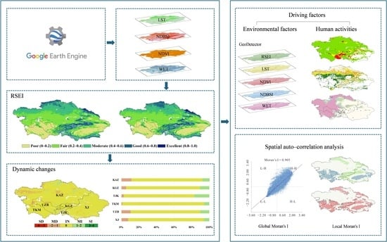
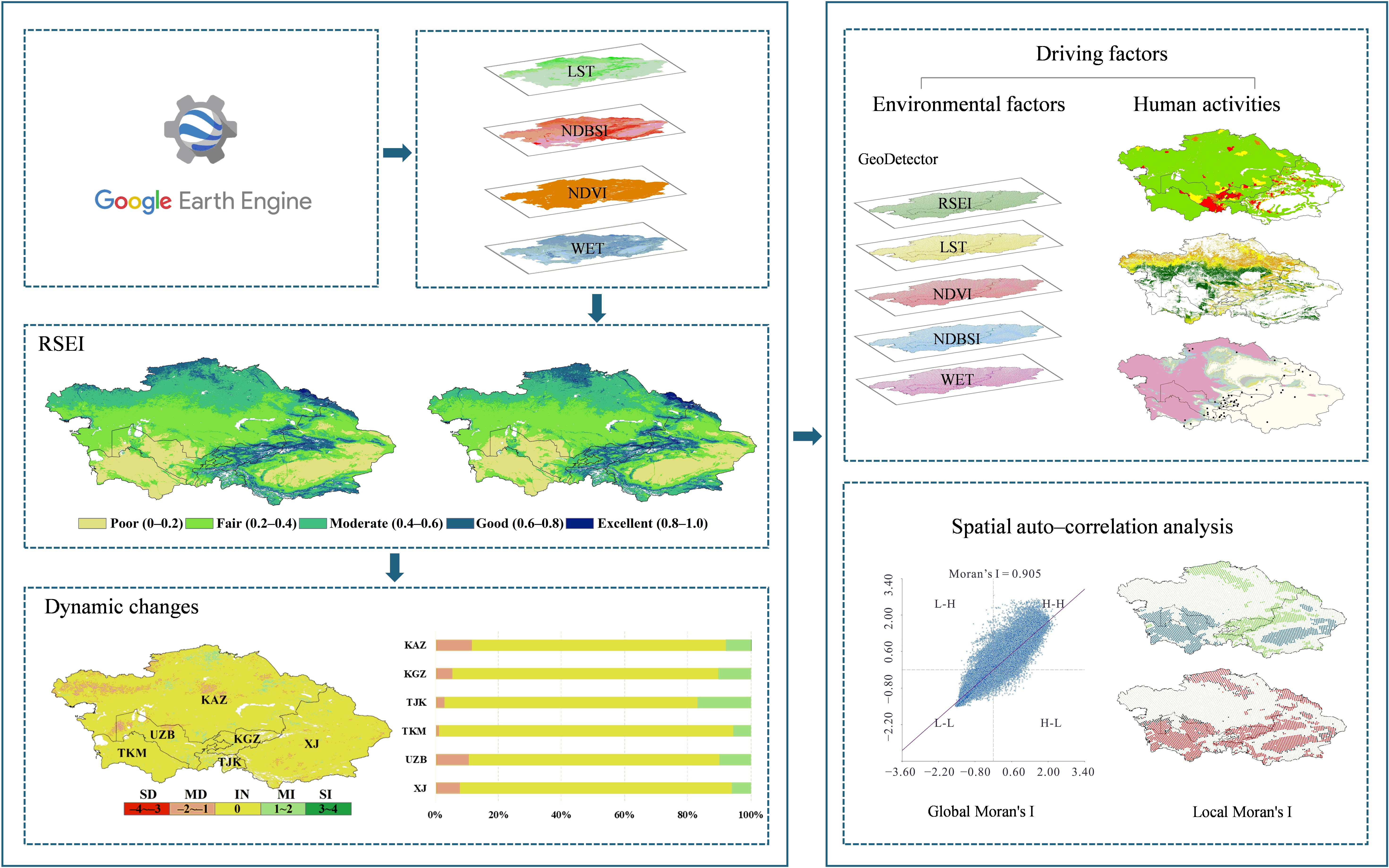
Maintaining the ecological security of arid Central Asia (CA) is essential for the sustainable development of arid CA. Based on the moderate-resolution imaging spectroradiometer (MODIS) data stored on the Google Earth Engine (GEE), this paper investigated the spatiotemporal changes and factors related to ecological environment quality (EEQ) in CA from 2000 to 2020 using the remote sensing ecological index (RSEI). The RSEI values in CA during 2000, 2005, 2010, 2015, and 2020 were 0.379, 0.376, 0.349, 0.360, and 0.327, respectively; the unchanged/improved/deteriorated areas during 2000–2005, 2005–2010, 2010–2015, and 2015–2020 were about 83.21/7.66%/9.13%, 77.28/6.68%/16.04%, 79.03/11.99%/8.98%, and 81.29/2.16%/16.55%, respectively, which indicated that the EEQ of CA was poor and presented a trend of gradual deterioration. Consistent with the RSEI trend, Moran’s I index values in 2000, 2005, 2010, 2015, and 2020 were 0.905, 0.893, 0.901, 0.898, and 0.884, respectively, revealing that the spatial distribution of the EEQ was clustered rather than random. The high–high (H-H) areas were mainly located in mountainous areas, and the low–low (L-L) areas were mainly distributed in deserts. Significant regions were mainly located in H-H and L-L, and most reached the significance level of 0.01, indicating that EEQ exhibited strong correlation. The EEQ in CA is affected by both natural and human factors. Among the natural factors, greenness and wetness promoted the EEQ, while heat and dryness reduced the EEQ, and heat had greater effects than the other three indexes. Human factors such as population growth, overgrazing, and hydropower development are important factors affecting the EEQ. This study provides important data for environmental protection and regional planning in arid and semi-arid regions.

1. Introduction

Ongoing rapid climate change and intensifying human activities have significant impacts on the global ecosystem, especially in vulnerable dryland ecosystems [1,2,3]. Therefore, the environment in arid and semi-arid areas has received significant attention [4,5,6,7]. Ecological environment quality (EEQ) evaluation is an important tool to quantitatively evaluate the environment and also serves as a criterion for formulating sustainable plans or measures for regional environmental management.

Numerous methods have been used to evaluate the EEQ in recent years [8,9,10,11,12,13,14]. However, methods that use only one indicator in the evaluation of the EEQ usually fail to include the complexity and diversity of the eco-environment and make the evaluation incomprehensive [15]. To achieve a comprehensive understanding of the EEQ, composite indicators have been widely used in the evaluation of the EEQ in recent years [16,17,18]. Among these composite indicators, the environmental index based on remote sensing information [17], named the remote sensing ecological index (RSEI), has been widely accepted and used for ecological monitoring and evaluation [19,20,21,22,23]. The RSEI reflects the regional environment by integrating the greenness, humidity, heat, and dryness of the eco-environment through principal component transformation, which overcomes the limitation of using a single index and can quickly realize the comprehensive evaluation of regional environments [17]. However, it is complex and time consuming when applying the RSEI to large-scale environments and long-term changes. Therefore, previous studies on the RSEI mostly focused on small areas within a short time range [19,20,21,22,23].

The Google Earth Engine (GEE), a free cloud platform that can quickly process massive images, has become a good choice in recent years for large-scale and long-time calculation of the RSEI, and it has been found to be effective in different regions and ecosystems [24,25,26]. For example, based on the GEE platform, Yang et al. analyzed the spatiotemporal change of the EEQ of the Yangtze River Basin (1.8 × 10⁶ km²) in China in the past 20 years (2001–2019) [24]; Yang et al. analyzed the EEQ in the Yellow River Basin (0.8 × 10⁶ km²) in China during 1990–2019 [25], and Ji et al. analyzed the EEQ of the whole of China (9.6 × 10⁶ km²) during 2001–2020 [26]. Therefore, it is feasible to calculate the RSEI for large-scale and long-time EEQ evaluation based on the GEE platform.

Central Asia (CA) is one of the largest arid and semi-arid regions in the Northern Hemisphere [27] and also contains some of the most vulnerable and sensitive terrestrial ecosystems in the world [28,29]. In recent years, climate change and anthropogenic activities have caused unprecedented damage to the ecosystems there, threatening environmental sustainability [30,31,32,33]. As one of the world’s greatest ecological disasters, the Aral Sea crisis in CA, in which the Aral Sea shrunk and largely disappeared after water was diverted for irrigation, led to desertification, and the resulting reduction in biodiversity has caused serious damage to the surrounding ecosystem [34,35]. Therefore, maintaining ecological security is of great significance to the ecological environment construction of arid CA and even the world. On the above basis, the objectives of this study were: (1) to construct the RSEI efficiently by MODIS sensing data based on the GEE platform; (2) to monitor spatial–temporal changes of the EEQ in CA from 2000 to 2020; and (3) to explore the spatial autocorrelation and identify the driving factors of the EEQ in CA. Our study provides a practical and economical approach for assessing spatial–temporal changes of the ecological environment quality based on RSEI and GEE.

2. Study Area

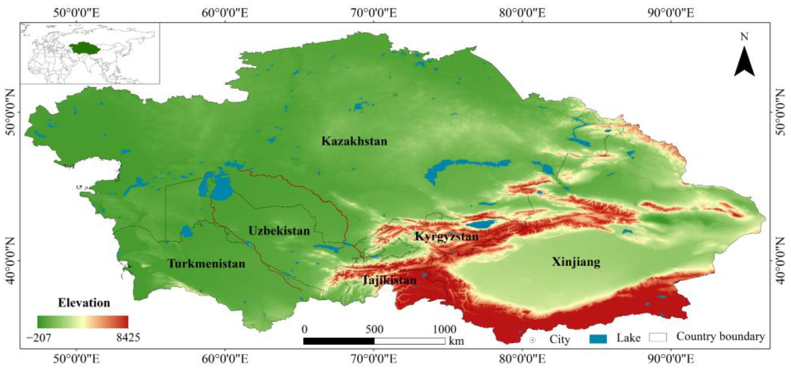
The CA region (46.50°E–87.35°E and 35.10°N–55.45°N) consists of the Xinjiang Uygur Autonomous Region (XJ) in northwest China and the five post-Soviet Union republics, namely, Kazakhstan (KAZ), Kyrgyzstan (KGZ), Tajikistan (TJK), Turkmenistan (TKM), and Uzbekistan (UZB). These nations and regions have a total area of 5.63 × 10⁶ km² and share the same ecological systems (Figure 1). Far from oceans, the CA region is characterized by a typical continental arid and semi-arid climate [36]. The annual average precipitation varies from 155 mm to 270 mm, whereas the annual average evaporation is between 900 mm and 1500 mm [37].

3. Data and Methodology

3.1. Data Collection

The products of MOD09A1 V6, MOD11A2 V6, and MOD13A1 V6 covering CA from June to September of 2000, 2005, 2010, 2015, and 2020 were obtained to map the RSEI. The Global Reservoir and Dam Database (GRanD) v1.3 (http://globaldamwatch.org/grand/, accessed on 8 May 2022), the Gridded Population of the World (GPW) v4 (https://0-doi-org.brum.beds.ac.uk/10.7927/H4F47M65, accessed on 8 May 2022), and the utilization intensity index of the main grazing grasslands in Eurasia (https://www.chinageoss.cn/geoarc/2021/index.html, accessed on 8 May 2022) were used to analyze the influence caused by associated driving factors.

3.2. Methods

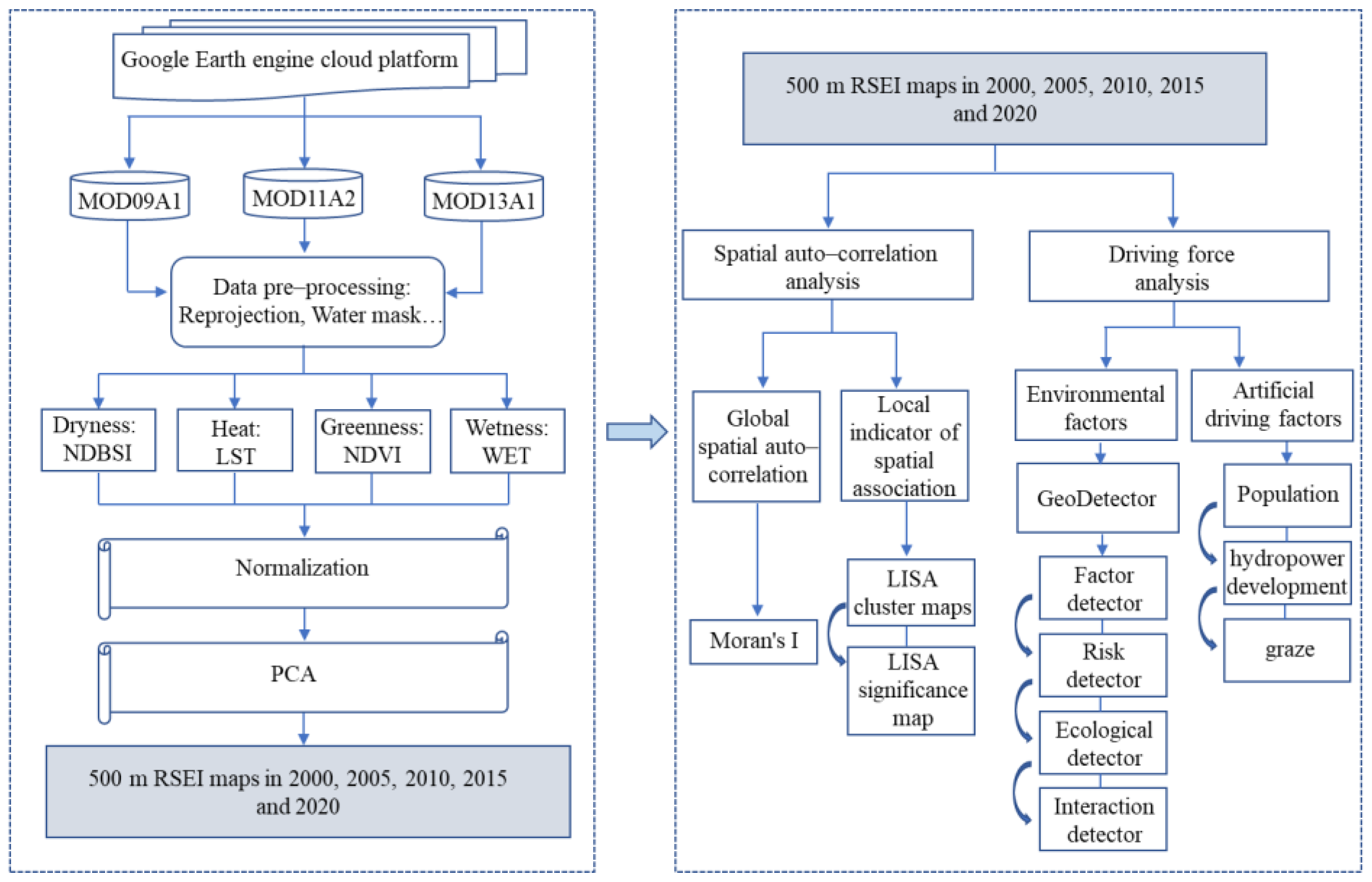
The study workflow is shown in Figure 2. The process used was as follows: (1) based on the GEE, four remote sensing indicators were calculated, namely, the land surface temperature (LST), the normalized difference impervious surface index (NDBSI), the normalized difference vegetation index (NDVI), and the wetness (WET); (2) spatial and temporal distributions of RSEIs for CA in 2000, 2005, 2010, 2015, and 2020 were generated using the principal component analysis (PCA) module in GEE; and (3) spatial auto-correlation analysis was applied to analyze the spatial correlation, and the geographical detector model (GDM) was used to quantitatively analyze the driving factors.

3.2.1. Methods of RSEI

As a recently developed comprehensive ecological index, the RSEI is specifically used to assess the EEQ with remote sensing data because it can reflect the pressures on the environment caused by human activities (i.e., urbanization), changes in the environmental state (i.e., vegetation coverage), and the climate change responses (i.e., temperatures and humidity) [11]. In this process, we calculated four component indicators (heat (LST), dryness (NDBSI), greenness (NDVI), and wetness (WET)) using MODIS data [38] and the GEE cloud platform.

The MODIS data were preprocessed to remove clouds and mask the water body before being processed. The NDVI was selected from the MOD13A1 product, the LST was selected from the MOD11A2 product, and the WET and NDBSI were calculated by the MOD09A1 image band [38].

Considering that the units and magnitudes of above indicators are not uniform, these indicators are normalized by Equation (1) before PCA, and their values are normalized to [0, 1]. After normalization, the four indicators were synthesized into new images, and the initial RSEI₀ was calculated by Equation (2). To facilitate the comparison of the four indicators, RSEI₀ can also be normalized with Equation (3) [17]. Equations (1) through (3) are as follows:

$${\mathit{NI}}_i{=(I}_i-I_{\mathit{min}}{)/(I}_{\mathit{max}}-I_{\mathit{min}})$$

(1)

$${\mathit{RSEI}}_0=1-{\mathit{PC}}_1\left[f\right(\mathit{Greenness},\mathit{Wetness},\mathit{Dryness},\mathit{Heat}\left)\right]$$

(2)

$${\mathit{RSEI}=(\mathit{RSEI}}_0-{\mathit{RSEI}}_{0_{\mathit{min}}}{)/(\mathit{RSEI}}_{0_{\mathit{max}}}-{\mathit{RSEI}}_{0_{\mathit{min}}})$$

(3)

where NI_i is the image standardization result of the indicator, I_i is the i pixel value of the indicator, I_max is the maximum value of the indicator in the target year, I_min is the minimum value of the indicator in the target year, PC1 is the first principal component, f is the forward normalization of the four indicators, and ${\mathit{RSEI}}_{0_{\mathit{max}}}$ and ${\mathit{RSEI}}_{0_{\mathit{min}}}$ are the maximum and minimum values of RSEI₀ for the target year, respectively.

3.2.2. Spatial Auto-Correlation Analysis

Spatial auto-correlation measures and tests the correlation between an element’s attribute value and that of its adjacent space [39,40]. This reveals an attribute eigenvalue correlation between the spatial reference unit and the adjacent spatial unit. In this paper, we analyzed the global and local spatial correlation of the RSEI using Global Moran’s I and Local Moran’s I separately [19].

3.2.3. GDM

The GDM integrates various statistical methods to detect the driving forces of factors, and it has been widely used in the detection of geographical environmental or human factors responsible for the changes of the EEQ [41,42,43,44]. In this study, the GDM was used to quantify the impacts of the LST, NDVI, NDBSI, and WET and their interactions on the RSEI of CA. A detailed description of the GDM was published by Wang and Xu [45].

4. Results

This paper used the GEE platform’s PCA module to quantitatively invert the RSEI for every 5 years during 2000–2020 of CA. The PCA results of CA and its six regions (

Table 1. Results of PCA for four indicators.

Year	Indicator	CA	KAZ	KGZ	TJK	TKM	UZB	XJ
2000	LST	−0.87	−0.71	0.97	0.94	−0.84	−0.75	−0.95
	NDBSI	0.00	−0.15	0.00	0.00	−0.04	−0.05	−0.01
	NDVI	0.45	0.66	0.00	0.13	0.27	0.44	0.27
	WET	0.19	0.21	−0.23	−0.33	0.48	0.50	0.16
	EV1	0.04	0.05	0.05	0.01	0.03	0.06	0.05
	EV2	0.00	0.02	0.02	0.00	0.01	0.01	0.01
	ECR1	79.51	85.67	68.30	70.54	62.95	74.12	80.35
	ECR2	17.05	8.92	26.96	22.22	21.51	16.30	15.66
2005	LST	−0.82	−0.70	−0.97	0.93	−0.80	−0.76	−0.92
	NDBSI	0.00	−0.01	0.00	0.01	−0.01	−0.02	−0.01
	NDVI	0.53	0.68	−0.07	0.12	0.32	0.47	0.34
	WET	0.21	0.22	0.23	−0.36	0.51	0.46	0.21
	EV1	0.04	0.05	0.06	0.01	0.03	0.06	0.05
	EV2	0.00	0.03	0.02	0.00	0.01	0.02	0.01
	ECR1	76.97	87.52	60.84	69.79	65.31	78.67	76.00
	ECR2	19.57	8.96	34.55	23.93	19.06	13.77	18.86
2010	LST	−0.87	−0.70	−0.95	0.90	−0.72	−0.70	−0.92
	NDBSI	0.00	−0.12	0.00	0.01	−0.06	−0.02	0.00
	NDVI	0.44	0.65	−0.15	0.23	0.32	0.53	0.33
	WET	0.24	0.27	0.29	−0.37	0.61	0.48	0.21
	EV1	0.03	0.05	0.07	0.02	0.04	0.06	0.04
	EV2	0.00	0.03	0.03	0.00	0.01	0.02	0.01
	ECR1	76.58	85.33	60.63	67.51	67.26	78.84	75.82
	ECR2	19.61	10.04	33.76	26.80	20.57	14.08	19.30
2015	LST	−0.83	−0.72	−0.95	0.93	−0.74	−0.70	−0.89
	NDBSI	0.00	−0.03	0.00	0.01	−0.01	0.00	−0.01
	NDVI	0.49	0.65	−0.04	0.12	0.35	0.51	0.38
	WET	0.25	0.24	0.31	−0.34	0.58	0.50	0.24
	EV1	0.04	0.05	0.06	0.02	0.04	0.06	0.05
	EV2	0.00	0.02	0.02	0.01	0.01	0.02	0.01
	ECR1	77.97	89.10	64.07	65.64	66.14	78.87	74.23
	ECR2	18.01	7.42	29.99	27.60	22.03	13.01	20.35
2020	LST	−0.78	−0.64	−0.87	−0.84	−0.55	−0.58	−0.83
	NDBSI	0.00	−0.19	0.00	0.00	0.00	0.00	0.00
	NDVI	0.45	0.63	−0.04	−0.07	0.27	0.43	0.39
	WET	0.42	0.39	0.49	0.53	0.79	0.69	0.41
	EV1	0.04	0.06	0.07	0.02	0.05	0.06	0.05
	EV2	0.00	0.02	0.02	0.01	0.01	0.01	0.01
	ECR1	76.11	82.65	63.50	70.12	70.55	79.99	72.00
	ECR2	14.71	8.73	25.29	18.84	21.83	12.38	15.91

Note: EV1: eigenvalue of Principal Component 1; EV2: eigenvalue of Principal Component 2; ECR1: contribution rate of Principal Component 1; ECR2: contribution rate of Principal Component 2; The values correspond to indicators is the result of eigenvectors.

) showed that (1) the sum of the first principal component (PC1) and the second principal component (PC2) eigen contribution rates for CA and its six regions exceeded 80. Therefore, the weighted superposition of the results of the first two principal components can be represented by most features of the LST, NDBSI, NDVI, and WET; (2) the PC contribution rate of CA was consistent with its six regions, indicating that the RSEI obtained from MODIS images was fit for large-scale EEQ evaluation; and (3) NDVI and WET promoted the ecological benefits; however, the NDBSI and LST do the opposite.

4.1. Dynamic Changes in the EEQ of CA

According to the classification labels reported by Xu [17], during the monitoring period (2000, 2005, 2010, 2015, and 2020), the EEQ levels of CA were mainly poor, fair, and moderate (Figure 3a–f,

Table 2. Area and percentage change of each RSEI level in CA and its six regions.

	RSEI Level	2000	2005	2010	2015	2020
CA	poor	20.90%	21.75%	22.16%	23.94%	28.50%
	fair	37.67%	38.37%	45.56%	39.71%	39.91%
	moderate	29.11%	27.00%	21.02%	23.99%	23.59%
	good	11.66%	11.89%	10.27%	11.52%	7.84%
	excellent	0.66%	0.99%	0.98%	0.85%	0.17%
KAZ	poor	2.99%	3.25%	5.18%	6.31%	11.66%
	fair	47.22%	51.74%	66.79%	55.85%	56.11%
	moderate	39.98%	34.42%	22.89%	28.18%	27.14%
	good	9.25%	9.43%	4.32%	8.54%	4.85%
	excellent	0.57%	1.17%	0.82%	1.11%	0.24%
KGZ	poor	0.00%	0.00%	0.00%	0.02%	0.09%
	fair	10.21%	7.45%	4.49%	11.50%	11.59%
	moderate	31.17%	32.88%	27.90%	34.97%	36.11%
	good	55.76%	56.23%	60.99%	51.62%	51.60%
	excellent	2.86%	3.44%	6.61%	1.88%	0.61%
TJK	poor	4.61%	3.02%	2.78%	4.59%	6.06%
	fair	24.18%	20.28%	15.80%	20.61%	25.54%
	moderate	49.93%	48.63%	42.35%	46.68%	49.84%
	good	21.25%	27.84%	37.39%	28.00%	18.54%
	excellent	0.03%	0.23%	1.68%	0.13%	0.02%
TKM	poor	79.86%	77.01%	82.95%	82.09%	84.83%
	fair	17.89%	19.26%	13.87%	14.41%	12.70%
	moderate	2.24%	3.72%	3.16%	3.46%	2.36%
	good	0.01%	0.02%	0.02%	0.04%	0.10%
	excellent	0.00%	0.00%	0.00%	0.00%	0.00%
UZB	poor	48.22%	53.36%	57.85%	59.00%	63.25%
	fair	35.90%	26.75%	22.48%	23.25%	19.78%
	moderate	15.34%	18.36%	17.84%	16.69%	16.22%
	good	0.54%	1.52%	1.83%	1.06%	0.74%
	excellent	0.00%	0.00%	0.01%	0.00%	0.00%
XJ	poor	29.74%	31.72%	26.85%	30.89%	35.46%
	fair	32.14%	29.69%	32.60%	29.29%	30.67%
	moderate	20.71%	21.42%	21.59%	22.00%	22.45%
	good	16.40%	16.13%	17.82%	16.99%	11.29%
	excellent	1.01%	1.03%	1.13%	0.83%	0.13%

). The RSEI in CA presented obvious spatial differentiation (Figure 3f); fair EEQ levels were found in the largest area, accounting for 40.25% of the total area, while moderate and poor EEQ levels accounted for 24.94% and 23.45% of the total area, respectively. The proportion of good EEQ levels was relatively small at 10.63%, and excellent EEQ levels accounted for only 0.73% of the total area. As shown in Table 2, from 2000 to 2020, the proportion of areas of the poor and fair was gradually increasing, and the proportion of areas below fair was over 87%, indicating that the overall ecological level of CA was poor and exhibited a deterioration trend.

Among the six regions in CA (Figure 3a–f, Table 2), (1) KGZ and TJK had the best ecological status, with high proportions of excellent, good, and moderate ecological quality and over 68.40% of their combined total areas classified as moderate or better; (2) TKM and UZB, located in the southwest of CA, had the worst ecological conditions, with poor ecological quality predominating in the majority of areas and accounting for 81.35% and 56.34% of TKM and UZB, respectively; and (3) KAZ and XJ had a high proportion of fair and moderate ecological quality areas, lending them overall moderate ecological status.

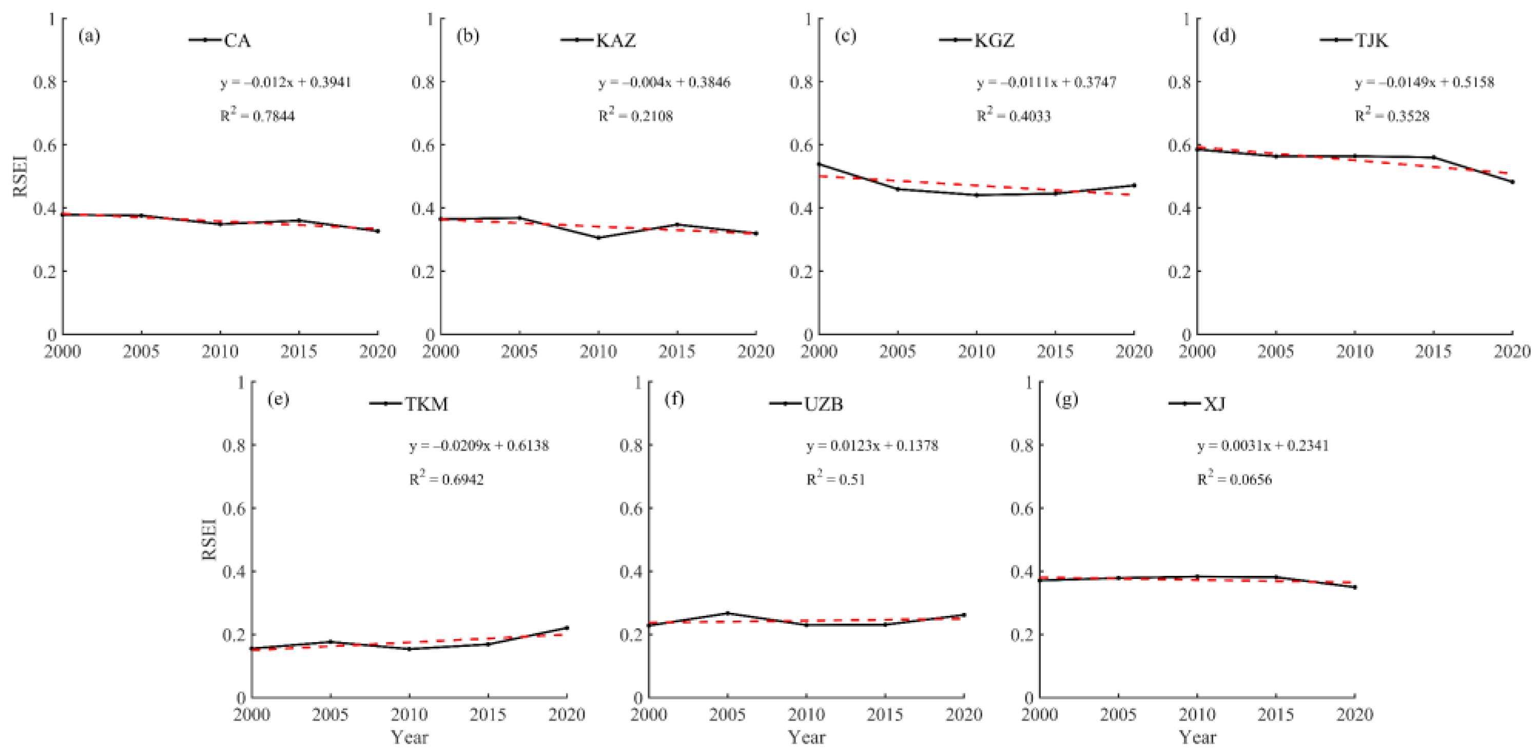
The mean values of the RSEI in CA and its six regions were calculated (Figure 4), with the following findings: (1) the level of ecological status in CA from 2000 to 2020 was fair, and the average value of the RSEI was between 0.327 and 0.394, with a decrease rate of 0.027/year, suggesting that the environment in CA was deteriorating (Figure 4a); (2) the EEQ grades of KGZ (0.471) and TJK (0.551) were moderate, the EEQ grades of KAZ (0.341), UZB (0.243), and XJ (0.373) were fair, and the EEQ grade of TKM was poor (0.175) (Figure 4b–g); (3) in the past 20 years, the RSEI of UZB and XJ showed an upward trend with increase rates of 0.012/year and 0.003/year, respectively, indicating that the ecological status improved (Figure 4f–g). KAZ, KGZ, TJK, and TKM showed a decreasing trend with decrease rates of 0.011/year, 0.020/year, 0.004/year, and 0.014/year, respectively, indicating that the ecological status was deteriorating (Figure 4b–e).

4.2. Spatiotemporal Characteristics of RSEI Evolution in CA

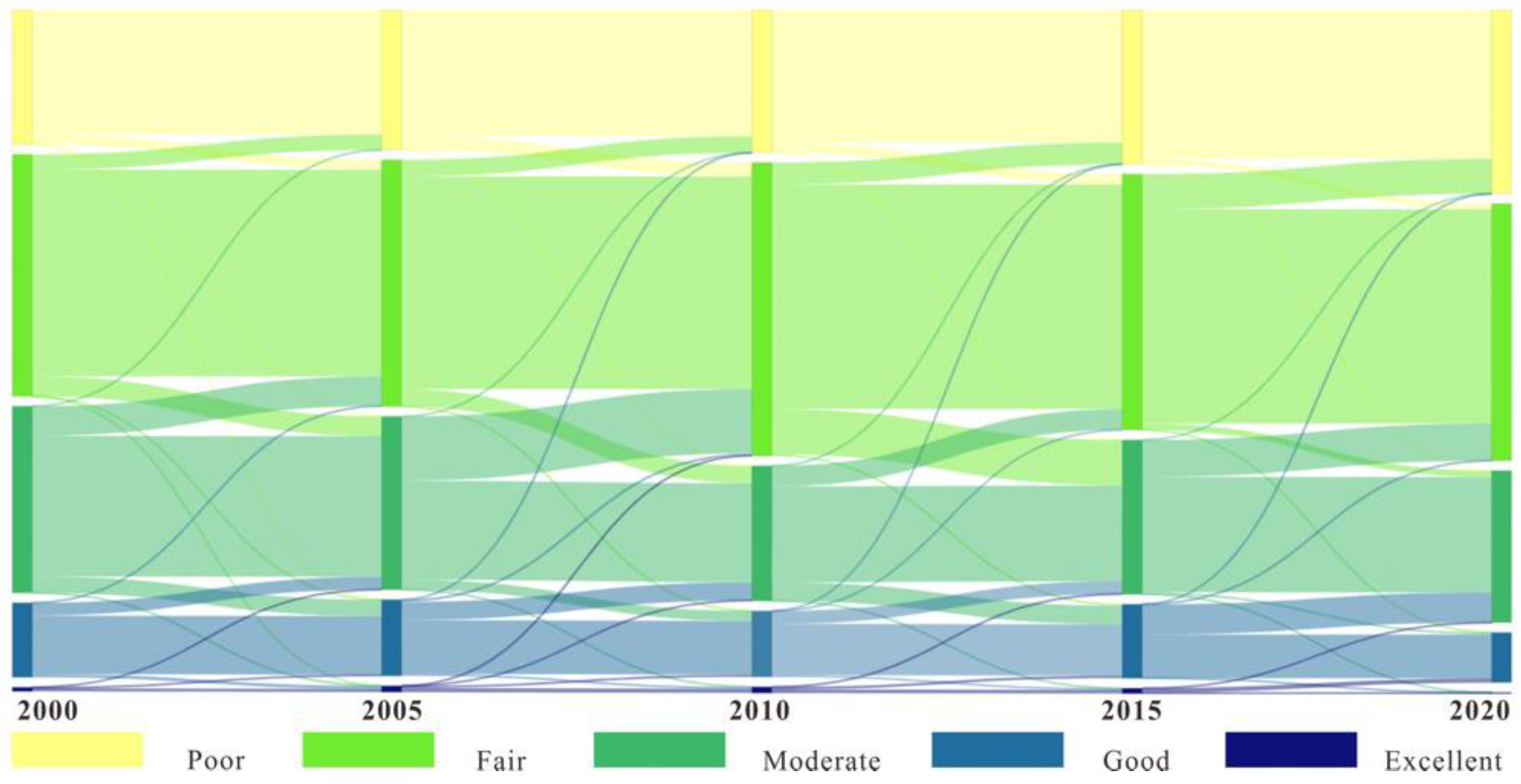
The spatiotemporal differences of the EEQ in CA were analyzed over four periods at 5-year intervals (2000–2005, 2005–2010, 2010–2015, and 2015–2020). The proportion of areas in which the RSEI remained unchanged in CA from 2000 to 2020 at about 80% (Figure 5). The proportions of improved areas in 2000–2005, 2005–2010, 2010–2015, and 2015–2020 were 7.66%, 6.68%, 11.99%, and 2.16%, respectively, showing a trend of decline. The proportions of deteriorated areas showed an opposite trend to that of improved areas, at 9.13%, 16.04%, 8.98%, and 16.55%, respectively. Although the overall EEQ of CA showed an unchanged trend from 2000 to 2020, more areas exhibited deterioration than improved areas, indicating that the EEQ of CA showed a gradual deterioration trend in recent years.

From the spatial distribution change of EEQ, although the EEQ in CA mainly remained unchanged in the four periods (2000–2005, 2005–2010, 2010–2015, and 2015–2020), the spatial distribution showed different characteristics in various periods (Figure 6a–d,

Table 3. Spatial distribution of changes in the EEQ of CA and its six regions in various periods.

Period	Region	SD	MD	IN	MI	SI
2000–2005	CA	0.00%	6.55%	83.97%	9.48%	0.00%
	KAZ	0.00%	11.62%	80.40%	7.98%	0.00%
	KGZ	0.00%	5.40%	84.33%	10.27%	0.00%
	TJK	0.00%	2.84%	80.24%	16.92%	0.00%
	TKM	0.00%	1.11%	93.32%	5.57%	0.00%
	UZB	0.00%	10.57%	79.36%	10.07%	0.00%
	XJ	0.00%	7.76%	86.16%	6.08%	0.00%
2005–2010	CA	0.00%	8.12%	83.04%	8.83%	0.00%
	KAZ	0.00%	27.78%	68.50%	3.72%	0.00%
	KGZ	0.00%	1.55%	83.09%	15.36%	0.00%
	TJK	0.00%	0.75%	81.07%	18.17%	0.00%
	TKM	0.00%	7.34%	91.95%	0.71%	0.00%
	UZB	0.00%	7.27%	90.45%	2.28%	0.00%
	XJ	0.00%	4.05%	83.20%	12.75%	0.00%
2010–2015	CA	0.00%	12.64%	81.90%	5.46%	0.00%
	KAZ	0.00%	6.73%	73.57%	19.70%	0.00%
	KGZ	0.00%	27.04%	72.00%	0.96%	0.00%
	TJK	0.00%	21.29%	78.35%	0.36%	0.00%
	TKM	0.00%	1.83%	95.05%	3.13%	0.00%
	UZB	0.01%	6.26%	91.52%	2.21%	0.00%
	XJ	0.00%	12.69%	80.90%	6.41%	0.00%
2015–2020	CA	0.00%	13.14%	84.42%	2.44%	0.00%
	KAZ	0.00%	18.37%	79.61%	2.01%	0.00%
	KGZ	0.00%	8.65%	86.01%	5.34%	0.00%
	TJK	0.00%	19.40%	78.78%	1.82%	0.00%
	TKM	0.00%	5.15%	93.60%	1.25%	0.00%
	UZB	0.00%	7.25%	91.03%	1.73%	0.00%
	XJ	0.00%	20.04%	77.49%	2.47%	0.00%

).

From 2000 to 2005, the areas of slight deterioration and slight improvement in CA showed sporadic distribution, and the area of slight improvement was larger than slight deterioration. The proportions of slightly deteriorated and slightly improved areas in KAZ, KGZ, TJK, TKM, UZB, and XJ were 11.62%/7.98%, 5.40%/10.27%, 2.84%/16.92%, 1.11%/5.57%, 10.57%/10.07%, and 7.76%/6.0, respectively (Figure 6a, Table 3).

Mild deterioration mainly occurred in northern KAZ from 2005 to 2010, and the areas of slight improvement were mainly located in KGZ, TJK, and XJ. The proportion of slightly deteriorated and slightly improved areas in KAZ, KGZ, TJK, TKM, UZB, and XJ was 27.78%/3.72%, 1.55%/15.36%, 0.75%/18.17%, 7.34%/0.71%, 7.27%/2.28%, and 4.05%/12.75, respectively (Figure 6b, Table 3).

From 2010 to 2015, slight improvement was mainly concentrated in northern KAZ, and the areas with mild deterioration were mainly located in KGZ, TJK, and XJ. In KAZ, KGZ, TJK, TKM, UZB, and XJ, the proportions of slightly deteriorated and slightly improved areas were 6.73%/19.70%, 27.04%/0.96%, 21.29%/0.36%, 1.83%/3.13%, 6.26%/2.21%, and 12.69%/6.41, respectively (Figure 6c, Table 3).

The spatial–temporal distribution of EEQ in CA during 2015–2020 showed similar sporadic distribution characteristics to that from 2000 to 2005, but the areas with slight deterioration were all larger than those with slight improvement. In KAZ, KGZ, TJK, TKM, UZB, and XJ, the proportions of slightly deteriorated and slightly improved areas were 18.37%/2.01%, 8.65%/5.34%, 19.40%/1.82%, 5.15%/1.25%, 7.25%/1.73%, and 20.04%/2.47%, respectively (Figure 6d, Table 3).

5. Discussion

5.1. Spatial Autocorrelation Analysis of EEQ

Spatial statistical analysis helps to understand ecological patterns and regional agglomerations [15,19]. In this study, the pixel size of the RSEI images from 2000, 2005, 2010, 2015, and 2020 were resampled to a 5 km × 5 km scale, and a total of 225,449 sample points were collected to determine whether the variables were spatially correlated and their extent. The spatial autocorrelation was analyzed using Moran’s I index and LISA diagram.

Figure 7 shows Moran’s I scatter diagram of the RSEI, which is mainly distributed in the first and third quadrants of each year, indicating a strong positive spatial correlation of environmental quality in the study area. Moran’s I index values for 2000, 2005, 2010, 2015, and 2020 were 0.905, 0.893, 0.901, 0.898, and 0.884, respectively, indicating that the spatial distribution of EEQ in the whole CA was clustered rather than random over the years. Moran’s I value decreased gradually from 2000 to 2020, which was consistent with the change of the EEQ grade (Figure 5).

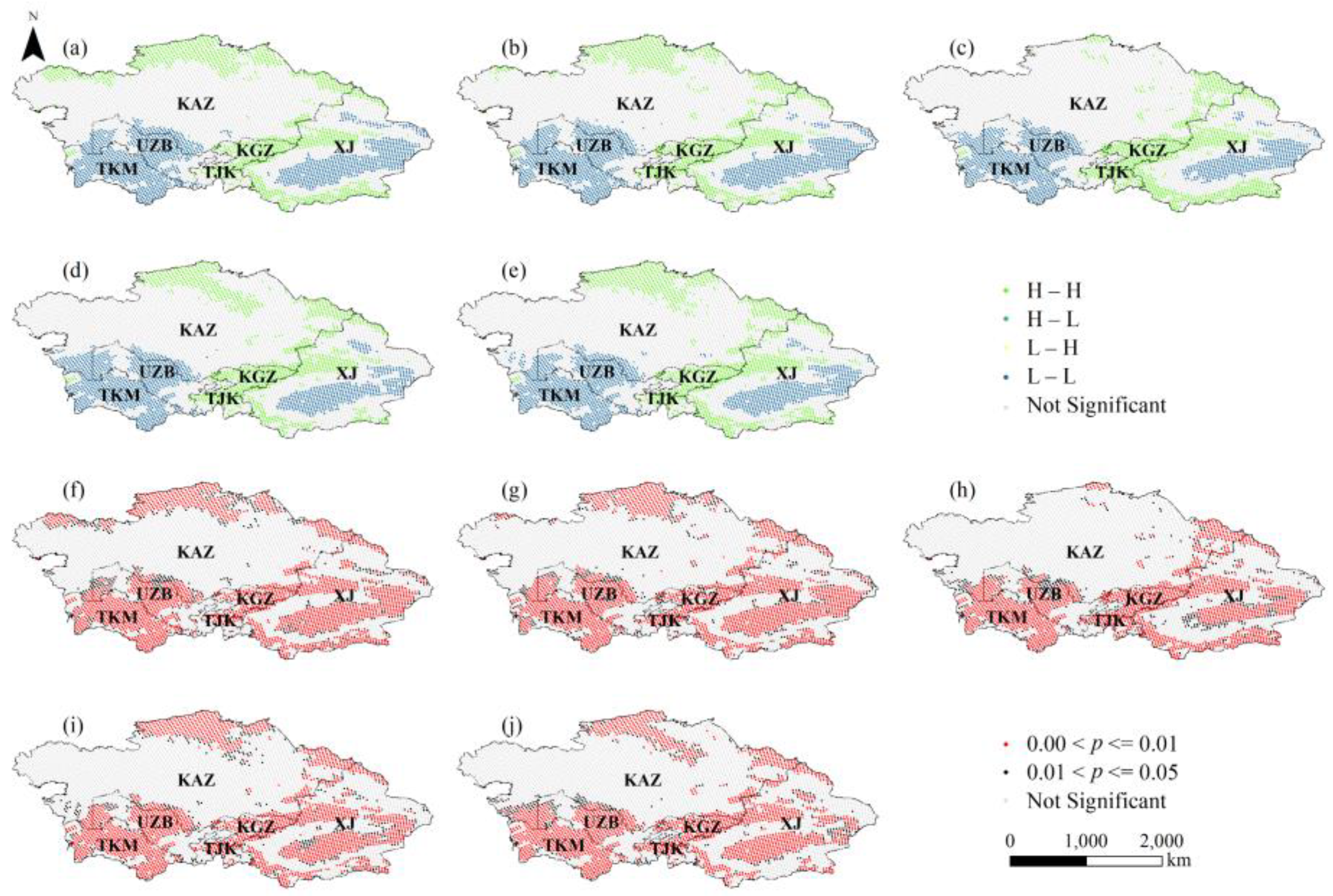
The local spatial correlation patterns of the EEQ were analyzed by the LISA cluster and the LISA significance level. As shown in the LISA clustering diagram (Figure 8), insignificant areas were mainly concentrated in the central and southern areas of KAZ and in the edge region of XJ. The high–high (H-H) clustering regions were mainly concentrated in the mountainous areas of KAZ, KGZ, TGK, and XJ. In 2010, the H-H distribution area of KAZ decreased, and the EEQ was poor. From 2015 to 2020, the H-H agglomeration area increased, and the ecological environment was good. The low–low (L-L) areas were mainly distributed in desert areas, such as the Taklimakan Desert in XJ, the Kyzyl-Kum Desert in UZB, and the Karakum Desert in TKM. These areas are characterized by scarce precipitation, high evaporation, and poor EEQ. The LISA cluster map directly reflected the spatial distribution of “H-H,” “L-L,” “high–low (H-L),” and “low–high (L-H),” and the LISA significant level map reflected the spatial significance level of environmental quality. The significant regions for 2000–2020 were mainly located in the H-H and L-L regions, most of which reached a significance level of 0.01, indicating a strong correlation of EEQ.

5.2. Impacts of Driving Factors on RSEI

The RSEI has been widely used to evaluate the EEQ in a variety of landscapes. RSEI values vary from landscape to landscape. Reported RSEI values include 0.18 in areas of severe soil erosion [46], 0.24 in desert areas [47,48], 0.27–0.68 in cities [11], 0.43–0.54 in tableland regions [49], 0.45–0.61 in islands [50], 0.49–0.69 in floodplains or the basins of large rivers [51], over 0.63 in forested/dense vegetation areas, and over 0.83 in good farmland [52]. In the present study, the RSEI ranged from 0.327 to 0.394. This value was at or near the values found in desert areas or cities, which correspond to the actual situation. The mean RSEI of CA ranged from 0.327 to 0.394 during 2000–2020, which might be closely related to changes in environmental factors and human interference.

5.2.1. Impacts of Natural Factors on RSEI

The GDM was applied to further reveal the dominant natural factors for the changes in the EEQ. The specific operation steps were as follows: four indicator images in the monitoring years (2000, 2005, 2010, 2015, and 2020) were resampled to 5 km × 5 km, and 225,449 points were generated in each image; the RSEI was taken as the independent variable, and four indicators were selected as the dependent variables; factor detection, ecological detection, interactive detection, and risk detection were carried out by matching the RSEI points with four index factor (LST, NDBSI, NDVI, and WET) points.

Factor detection was used to calculate the p-value of each factor to explore whether each factor had an impact on RSEI and its contribution rate [45]. According to the factor detection results, the p-values of the four indicators in CA and the six regions were less than 0.01, passing the significance test. The contribution rate of the LST was over 90%, which was higher than the other three factors (about 50%). Therefore, while the NDVI, NDBSI, LST, and WET all have significant effects on the EEQ of CA and its six regions, the LST is the main factor.

Ecological detectors were used to determine if there was a significant difference between two factors of the RSEI [45]. The results showed that although the difference between the two factors was significant in different years, the spatial distributions of the RSEI in CA and the six regions were mostly affected by the LST.

By calculating the p-value of the interaction between two natural factors, the interactive detector analyzes whether the two natural factors interact or are independent [45]. The interaction results of each of the two main influencing factors in CA and its six regions exhibited two-factor enhancement, and there was no independent factor, indicating that there was an interaction between two factors and it was not a simple superposition.

The risk detector can determine the best range partition or feature through which different factors promote RSEI growth, with a confidence level of 95%. The risk detection results of each factor could be divided into two parts: the statistical difference between different regions and the mean value of the RSEI [45]. The results showed that the mean value of the RSEI was negatively correlated with the LST and NDBSI, that is, the smaller the range of the LST and NDBSI, the larger the RSEI value. In contrast, the RSEI was positively correlated with the NDVI and WET; in other words, the larger the range of the NDVI and WET, the greater the RSEI value. This was consistent with the PCA results. In addition, statistical tests showed that the optimal region of the RSEI for each factor was significantly different from other regions, which further demonstrated that each factor could better promote the growth of the RSEI in the optimal region.

5.2.2. Impacts of Human Activities on RSEI

CA is typically arid and semi-arid and consists of a very fragile ecological environment, making it particularly sensitive and vulnerable to human disturbance [53,54]. Previous studies have shown primarily shrinkage in the Aral Sea basin due to diversion of rivers for agricultural irrigation [55] and construction of reservoirs [56]. Wang et al. confirmed a greater impact of human activities than climate change [57].

In recent years, large-scale human activities in CA have had an important impact on the local environment. For example, the population of CA and its six regions has shown a continuous growth trend, especially TJK and UZB, with population growth rates of 5.67 persons/km²/y and 5.17 persons/km²/y, respectively (Figure 9a). According to the Global Reservoir and Dam Database (GranD) v1.3, more than 40 large dams and reservoirs have been built over the last 30 years in CA (Figure 9a), significantly affecting the surrounding ecosystem [58]. The spatial distribution of the utilization intensity index of the main grazing grasslands in CA also showed an increasing trend. Areas with high utilization intensity index were mainly distributed in the north and east of KAZ, and low-utilization areas were mainly distributed in the south of KAZ, the southeast of UZB, and central TKM, which was consistent with areas of degraded ecological quality (Figure 9b). Environmental protection measures have played a positive role in promoting the improvement of local EEQ. For example, the improvement of the EEQ in XJ in recent years was related to a series of local ecological protection measures [19].

5.3. Limitations and Future Work

In this paper, the rapid and efficient comparative analysis of the regional environment was achieved by integrating multi-source remote sensing data and using the GEE cloud platform. This method can provide support for regional development planning and the formulation of environmental protection measures. However, the environment in arid areas is fragile, and the environmental quality is sensitive to changes in natural environmental factors and human activities [57,59,60,61,62,63]. In addition to the LST, NDBSI, NDVI, and WET, global warming, soil erosion, desertification, a decrease in biodiversity, population surges, and the intensification of urbanization will all damage the environmental balance. In addition to these factors, the Tienshan Mountains in CA, are known as the “water tower of CA” [64]. However, the RSEI calculations did not take the effects of glacial change into account. In addition, to prevent the interference of large areas of water with actual surface humidity conditions, a water mask was adopted in the RSEI calculation process, as water areas play a crucial role in the environmental development in arid areas [65,66,67]. Therefore, the evaluation of the environment in CA should be conducted while considering local conditions to obtain more comprehensive and scientific evaluation results.

6. Conclusions

Based on the GEE cloud platform and MODIS data, the RSEI was used to study the spatiotemporal dynamics and changes of EEQ in CA and its six regions during 2000–2020 to explore the spatial correlation and the driving factors of the EEQ. The results were as follows.

(1)

The RSEI values in CA during 2000, 2005, 2010, 2015, and 2020 were 0.379, 0.376, 0.349, 0.360, and 0.327, respectively, revealing that the EEQ was at a poor level and showed a deteriorating trend. Among the six regions of CA, although UZB and XJ had medium EEQ grades of fair, both of these regions showed a trend of improvement. KGZ and TJK had the best EEQ grades of moderate, KAZ had a medium EEQ grade of fair, and TKM had the worst EEQ grade of poor; all of these regions showed a trend of deterioration.

(2)

During 2000–2005, 2005–2010, 2010–2015, and 2015–2020, the unchanged/improved/deteriorated areas in CA were about 83.21/7.66%/9.13%, 77.28/6.68%/16.04%, 79.03/11.99%/8.98%, and 81.29/2.16%/16.55%, respectively, indicating that the overall EEQ in CA gradually deteriorated in recent years. The six regions of CA exhibited similar characteristics.

(3)

Analysis from Moran’s I index indicated that the spatial distribution of the EEQ in CA was clustered rather than random. Areas of H-H were mainly concentrated in mountainous areas, and L-L areas were mainly distributed in desert areas; the significant regions were mainly located in H-H and L-L areas, and most of them reached the significance level of 0.01, indicating that environmental quality had a strong correlation.

(4)

The results of the GDM revealed the influence of natural factors on the EEQ in CA. The findings showed that, although all factors had an impact on the RSEI in CA and its six regions, LST was the main factor. The impacts of various factors on the RSEI were not a simple superposition process but rather a mutual enhancement. The LST and NDBSI had a negative correlation with the RSEI, whereas the NDVI and WET had a positive correlation with the RSEI. In addition, human activities, such as population growth, overgrazing, and hydropower development, had an important impact on the EEQ.

By writing programs in the GEE platform to directly access databases for data processing and analysis, the problem of low-efficiency steps such as local downloading, storage, and pre-processing can be overcome, and index calculation can be conducted quickly in the GEE cloud. Therefore, GEE can be used as a computing platform to evaluate the EEQ, and its application can be extended to evaluate the EEQ by the RSEI over a large range and long time series.

References

- Li, D.; Wu, S.; Liu, L.; Zhang, Y.; Li, S. Vulnerability of the global terrestrial ecosystems to climate change. Glob. Chang. Biol. 2018, 24, 4095–4106. [Google Scholar] [CrossRef]
- Huang, J.; Zhang, G.; Zhang, Y.; Guan, X.; Wei, Y.; Guo, R. Global desertification vulnerability to climate change and human activities. Land Degrad. Dev. 2020, 31, 1380–1391. [Google Scholar] [CrossRef]
- Mahmoud, S.H.; Gan, T.Y. Impact of anthropogenic climate change and human activities on environment and ecosystem services in arid regions. Sci. Total Environ. 2018, 633, 1329–1344. [Google Scholar] [CrossRef] [PubMed]
- Yeilagi, S.; Rezapour, S.; Asadzadeh, F. Degradation of soil quality by the waste leachate in a Mediterranean semi-arid ecosystem. Sci. Rep. 2021, 11, 11390. [Google Scholar] [CrossRef] [PubMed]
- Li, C.; Wang, Y.; Wu, X.; Cao, H.; Li, W.; Wu, T. Reducing human activity promotes environmental restoration in arid and semi-arid regions: A case study in Northwest China. Sci. Total Environ. 2021, 768, 144525. [Google Scholar] [CrossRef]
- Wu, Z.; Lei, S.; Yan, Q.; Bian, Z.; Lu, Q. Landscape ecological network construction controlling surface coal mining effect on landscape ecology: A case study of a mining city in semi-arid steppe. Ecol. Indic. 2021, 133, 108403. [Google Scholar] [CrossRef]
- Kumar, R.; Pande, V.C.; Bhardwaj, A.K.; Dinesh, D.; Bhatnagar, P.R.; Dobhal, S.; Sharma, S.; Verma, K. Long-term impacts of afforestation on biomass production, carbon stock, and climate resilience in a degraded semi-arid ravine ecosystem of India. Ecol. Eng. 2022, 177, 106559. [Google Scholar] [CrossRef]
- Sullivan, C.A.; Skeffington, M.S.; Gormally, M.J.; Finn, J.A. The ecological status of grasslands on lowland farmlands in western Ireland and implications for grassland classification and nature value assessment. Biol. Conserv. 2010, 143, 1529–1539. [Google Scholar] [CrossRef]
- Ochoa-Gaona, S.; Kampichler, C.; de Jong, B.H.J.; Hernandez, S.; Geissen, V.; Huerta, E. A multi-criterion index for the evaluation of local tropical forest conditions in Mexico. For. Ecol. Manag. 2010, 260, 618–627. [Google Scholar] [CrossRef]
- Wu, X.X.; Lv, M.; Jin, Z.Y.; Michishita, R.; Chen, J.; Tian, H.Y.; Tu, X.B.; Zhao, H.M.; Niu, Z.G.; Chen, X.L.; et al. Normalized difference vegetation index dynamic and spatiotemporal distribution of migratory birds in the Poyang Lake wetland, China. Ecol. Indic. 2014, 47, 219–230. [Google Scholar] [CrossRef]
- Hu, X.; Xu, H. A new remote sensing index for assessing the spatial heterogeneity in urban ecological quality: A case from Fuzhou City, China. Ecol. Indic. 2018, 89, 11–21. [Google Scholar] [CrossRef]
- Shan, W.; Jin, X.B.; Ren, J.; Wang, Y.C.; Xu, Z.G.; Fan, Y.T.; Gu, Z.M.; Hong, C.Q.; Lin, J.H.; Zhou, Y.K. Ecological environment quality assessment based on remote sensing data for land consolidation. J. Clean. Prod. 2019, 239, 118126. [Google Scholar] [CrossRef]
- Singh, R.K.; Khand, K.; Kagone, S.; Schauer, M.; Senay, G.B.; Wu, Z. A novel approach for next generation water-use mapping using Landsat and Sentinel-2 satellite data. Hydrol. Sci. J. J. Des Sci. Hydrol. 2020, 65, 2508–2519. [Google Scholar] [CrossRef]
- Wen, C.; Zhan, Q.; Zhan, D.; Zhao, H.; Yang, C. Spatiotemporal Evolution of Lakes under Rapid Urbanization: A Case Study in Wuhan, China. Water 2021, 13, 1171. [Google Scholar] [CrossRef]
- Xiong, Y.; Xu, W.; Lu, N.; Huang, S.; Wu, C.; Wang, L.; Dai, F.; Kou, W. Assessment of spatial-temporal changes of ecological environment quality based on RSEI and GEE: A case study in Erhai Lake Basin, Yunnan province, China. Ecol. Indic. 2021, 125, 107518. [Google Scholar] [CrossRef]
- Sun, D.; Zhang, J.; Zhu, C.; Hu, Y.; Zhou, L. An Assessment of China’s Ecological Environment Quality Change and Its Spatial Variation. Acta Geogr. Sin. 2012, 67, 1599–1610. [Google Scholar] [CrossRef]
- Xu, H. A remote sensing index for assessment of regional ecological changes. China Environ. Sci. 2013, 33, 889–897. [Google Scholar] [CrossRef]
- Yue, A.; Zhang, Z. Analysis and research on ecological situation change based on EI value. J. Green Sci. Technol. 2018, 14, 182–184. [Google Scholar] [CrossRef]
- Jing, Y.; Zhang, F.; He, Y.; Kung, H.-T.; Johnson, V.C.; Arikena, M. Assessment of spatial and temporal variation of ecological environment quality in Ebinur Lake Wetland National Nature Reserve, Xinjiang, China. Ecol. Indic. 2020, 110, 105874. [Google Scholar] [CrossRef]
- Yuan, B.; Fu, L.; Zou, Y.; Zhang, S.; Chen, X.; Li, F.; Deng, Z.; Xie, Y. Spatiotemporal change detection of ecological quality and the associated affecting factors in Dongting Lake Basin, based on RSEI. J. Clean. Prod. 2021, 302, 126995. [Google Scholar] [CrossRef]
- Liu, C.; Yang, M.; Hou, Y.; Zhao, Y.; Xue, X. Spatiotemporal evolution of island ecological quality under different urban densities: A comparative analysis of Xiamen and Kinmen Islands, southeast China. Ecol. Indic. 2021, 124, 107438. [Google Scholar] [CrossRef]
- Boori, M.S.; Choudhary, K.; Paringer, R.; Kupriyanov, A. Spatiotemporal ecological vulnerability analysis with statistical correlation based on satellite remote sensing in Samara, Russia. J. Environ. Manag. 2021, 285, 112138. [Google Scholar] [CrossRef] [PubMed]
- Ariken, M.; Zhang, F.; Liu, K.; Fang, C.L.; Kung, H.T. Coupling coordination analysis of urbanization and eco-environment in Yanqi Basin based on multi-source remote sensing data. Ecol. Indic. 2020, 114, 106331. [Google Scholar] [CrossRef]
- Yang, X.; Meng, F.; Fu, P.; Zhang, Y.; Liu, Y. Spatiotemporal change and driving factors of the Eco-Environment quality in the Yangtze River Basin from 2001 to 2019. Ecol. Indic. 2021, 131, 108214. [Google Scholar] [CrossRef]
- Yang, Z.; Tian, J.; Li, W.; Su, W.; Guo, R.; Liu, W. Spatio-temporal pattern and evolution trend of ecological environment quality in the Yellow River Basin. Acta Ecol. Sin. 2021, 41, 7627–7636. [Google Scholar] [CrossRef]
- Ji, J.; Tang, Z.; Zhang, W.; Liu, W.; Jin, B.; Xi, X.; Wang, F.; Zhang, R.; Guo, B.; Xu, Z.; et al. Spatiotemporal and Multiscale Analysis of the Coupling Coordination Degree between Economic Development Equality and Eco-Environmental Quality in China from 2001 to 2020. Remote Sens. 2022, 14, 737. [Google Scholar] [CrossRef]
- Cowan, P.J. Geographic usage of the terms middle Asia and Central Asia. J. Arid. Environ. 2007, 69, 359–363. [Google Scholar] [CrossRef]
- Yao, J.; Hu, W.; Chen, Y.; Huo, W.; Zhao, Y.; Mao, W.; Yang, Q. Hydro-climatic changes and their impacts on vegetation in Xinjiang, Central Asia. Sci. Total Environ. 2019, 660, 724–732. [Google Scholar] [CrossRef] [PubMed]
- Bai, J.; Shi, H.; Yu, Q.; Xie, Z.; Li, L.; Luo, G.; Jin, N.; Li, J. Satellite-observed vegetation stability in response to changes in climate and total water storage in Central Asia. Sci. Total Environ. 2019, 659, 862–871. [Google Scholar] [CrossRef] [PubMed]
- Zhou, Y.; Zhang, L.; Fensholt, R.; Wang, K.; Vitkovskaya, I.; Tian, F. Climate Contributions to Vegetation Variations in Central Asian Drylands: Pre- and Post-USSR Collapse. Remote Sens. 2015, 7, 2449–2470. [Google Scholar] [CrossRef] [Green Version]
- Li, Z.; Chen, Y.N.; Li, W.H.; Deng, H.J.; Fang, G.H. Potential impacts of climate change on vegetation dynamics in Central Asia. J. Geophys. Res. Atmos. 2015, 120, 12345–12356. [Google Scholar] [CrossRef]
- Xu, H.; Wang, X.; Zhang, X. Decreased vegetation growth in response to summer drought in Central Asia from 2000 to 2012. Int. J. Appl. Earth Obs. Geoinf. 2016, 52, 390–402. [Google Scholar] [CrossRef]
- Jiang, L.L.; Jiapaer, G.; Bao, A.M.; Guo, H.; Ndayisaba, F. Vegetation dynamics and responses to climate change and human activities in Central Asia. Sci. Total Environ. 2017, 599, 967–980. [Google Scholar] [CrossRef] [PubMed]
- Wang, X.X.; Chen, Y.N.; Li, Z.; Fang, G.H.; Wang, F.; Liu, H.J. The impact of climate change and human activities on the Aral Sea Basin over the past 50 years. Atmos. Res. 2020, 245, 105125. [Google Scholar] [CrossRef]
- Berdimbetov, T.; Ma, Z.G.; Shelton, S.; Ilyas, S.; Nietullaeva, S. Identifying Land Degradation and its Driving Factors in the Aral Sea Basin from 1982 to 2015. Front. Earth Sci. 2021, 9, 834. [Google Scholar] [CrossRef]
- Lioubimtseva, E.; Cole, R.; Adams, J.; Kapustin, G. Impacts of climate and land-cover changes in arid lands of Central Asia. J. Arid. Environ. 2005, 62, 285–308. [Google Scholar] [CrossRef]
- Qin, J.; Hao, X.; Hua, D.; Hao, H. Assessment of ecosystem resilience in Central Asia. J. Arid. Environ. 2021, 195, 104625. [Google Scholar] [CrossRef]
- He, Y.; You, N.; Cui, Y.; Xiao, T.; Hao, Y.; Dong, J. Spatio-temporal changes in remote sensing-based ecological index in China since 2000. J. Nat. Resour. 2021, 36, 1176–1185. [Google Scholar] [CrossRef]
- Fan, G.Y.; Cowley, J.M. Auto-correlation analysis of high resolution electron micrographs of near-amorphous thin films. Ultramicroscopy 1985, 17, 345–355. [Google Scholar] [CrossRef]
- Martin, D. An assessment of surface and zonal models of population. Int. J. Geogr. Inf. Syst. 1996, 10, 973–989. [Google Scholar] [CrossRef]
- Liu, X.; Wang, H.; Wang, X.; Bai, M.; He, D. Driving factors and their interactions of carabid beetle distribution based on the geographical detector method. Ecol. Indic. 2021, 133, 108393. [Google Scholar] [CrossRef]
- Zhao, F.; Zhang, S.; Du, Q.; Ding, J.; Luan, G.; Xie, Z. Assessment of the sustainable development of rural minority settlements based on multidimensional data and geographical detector method: A case study in Dehong, China. Socio-Econ. Plan. Sci. 2021, 78, 101066. [Google Scholar] [CrossRef]
- Li, L.; Fan, Z.; Feng, W.; Yuxin, C.; Keyu, Q. Coupling coordination degree spatial analysis and driving factor between socio-economic and eco-environment in northern China. Ecol. Indic. 2022, 135, 108555. [Google Scholar] [CrossRef]
- Xiao, Z.; Liu, R.; Gao, Y.; Yang, Q.; Chen, J. Spatiotemporal variation characteristics of ecosystem health and its driving mechanism in the mountains of southwest China. J. Clean. Prod. 2022, 345, 131138. [Google Scholar] [CrossRef]
- Wang, J.; Xu, C. Geodetector: Principle and prospective. Acta Geogr. Sin. 2017, 72, 116–134. [Google Scholar] [CrossRef]
- Song, H.M.; Xue, L. Dynamic monitoring and analysis of ecological environment in Weinan City, Northwest China based on RSEI model. Chin. J. Appl. Ecol. 2016, 27, 3913–3919. [Google Scholar] [CrossRef]
- Jiang, C.L.; Wu, L.; Liu, D.; Wang, S.M. Dynamic monitoring of eco-environmental quality in arid desert area by remote sensing: Taking the Gurbantunggut Desert China as an example. Chin. J. Appl. Ecol. 2019, 30, 877–883. [Google Scholar] [CrossRef]
- Eyring, V.; Cox, P.M.; Flato, G.M.; Gleckler, P.J.; Abramowitz, G.; Caldwell, P.; Collins, W.D.; Gier, B.K.; Hall, A.D.; Hoffman, F.M.; et al. Taking climate model evaluation to the next level. Nat. Clim. Chang. 2019, 9, 102–110. [Google Scholar] [CrossRef] [Green Version]
- Sun, C.; Li, X.; Zhang, W.; Li, X. Evolution of ecological security in the tableland region of the Chinese Loess Plateau Using a remote-sensing-based index. Sustainability 2020, 12, 3489. [Google Scholar] [CrossRef] [Green Version]
- Wen, X.; Ming, Y.; Gao, Y.; Hu, X. Dynamic Monitoring and Analysis of Ecological Quality of Pingtan Comprehensive Experimental Zone, a New Type of Sea Island City, Based on RSEI. Sustainability 2020, 12, 21. [Google Scholar] [CrossRef] [Green Version]
- Zhu, Q.; Guo, J.; Guo, X.; Xu, Z.; Ding, H.; Han, Y. Spatial variation of ecological environment quality and its influencing factors in Poyang Lake area, Jiangxi, China. Chin. J. Appl. Ecol. 2019, 30, 4108–4116. [Google Scholar] [CrossRef]
- Wang, S.; Zhang, X.; Zhu, T.; Yang, W.; Zhao, J. Assessment of ecological environment quality in the Changbai Mountain Nature Reserve based on remote sensing technology. Prog. Geogr. 2016, 35, 1269–1278. [Google Scholar] [CrossRef]
- Loboda, T.V.; Giglio, L.; Boschetti, L.; Justice, C.O. Regional fire monitoring and characterization using global NASA MODIS fire products in dry lands of Central Asia. Front. Earth Sci. 2012, 6, 196–205. [Google Scholar] [CrossRef]
- Chen, T.; Tang, G.; Yuan, Y.; Guo, H.; Xu, Z.; Jiang, G.; Chen, X. Unraveling the relative impacts of climate change and human activities on grassland productivity in Central Asia over last three decades. Sci. Total Environ. 2020, 743, 140649. [Google Scholar] [CrossRef] [PubMed]
- Beek, T.A.D.; Voss, F.; Florke, M. Modelling the impact of Global Change on the hydrological system of the Aral Sea basin. Phys. Chem. Earth 2011, 36, 684–695. [Google Scholar] [CrossRef]
- Hall, J.W.; Grey, D.; Garrick, D.; Fung, F.; Brown, C.; Dadson, S.J.; Sadoff, C.W. Coping with the curse of freshwater variability. Science 2014, 346, 429–430. [Google Scholar] [CrossRef]
- Wang, J.; Liu, D.; Ma, J.; Cheng, Y.; Wang, L. Development of a large-scale remote sensing ecological index in arid areas and its application in the Aral Sea Basin. J. Arid. Land 2021, 13, 40–55. [Google Scholar] [CrossRef]
- Huang, W.; Duan, W.; Chen, Y. Rapidly declining surface and terrestrial water resources in Central Asia driven by socio-economic and climatic changes. Sci. Total Environ. 2021, 784, 147193. [Google Scholar] [CrossRef]
- Li, J.; Chen, Y.; Xu, C.; Li, Z. Evaluation and analysis of ecological security in arid areas of Central Asia based on the emergy ecological footprint (EEF) model. J. Clean. Prod. 2019, 235, 664–677. [Google Scholar] [CrossRef]
- Bi, X.; Chang, B.; Hou, F.; Yang, Z.; Fu, Q.; Li, B. Assessment of Spatio-Temporal Variation and Driving Mechanism of Ecological Environment Quality in the Arid Regions of Central Asia, Xinjiang. Int. J. Environ. Res. Public Health 2021, 18, 7111. [Google Scholar] [CrossRef]
- Yang, L.; Shi, L.; Wei, J.; Wang, Y. Spatiotemporal evolution of ecological environment quality in arid areas based on the remote sensing ecological distance index: A case study of Yuyang district in Yulin city, China. Open Geosci. 2021, 13, 1701–1710. [Google Scholar] [CrossRef]
- Sun, L.; Yu, Y.; Gao, Y.; He, J.; Yu, X.; Malik, I.; Wistuba, M.; Yu, R. Remote Sensing Monitoring and Evaluation of the Temporal and Spatial Changes in the Eco-Environment of a Typical Arid Land of the Tarim Basin in Western China. Land 2021, 10, 868. [Google Scholar] [CrossRef]
- Wu, S.; Gao, X.; Lei, J.; Zhou, N.; Guo, Z.; Shang, B. Ecological environment quality evaluation of the Sahel region in Africa based on remote sensing ecological index. J. Arid. Land 2022, 14, 14–33. [Google Scholar] [CrossRef]
- Chen, Y.N.; Li, W.H.; Deng, H.J.; Fang, G.H.; Li, Z. Changes in Central Asia’s Water Tower: Past, Present and Future. Sci. Rep. 2016, 6, 35458. [Google Scholar] [CrossRef] [PubMed]
- Zhang, Y.; Liu, W.; Cai, Y.; Khan, S.U.; Zhao, M. Decoupling analysis of water use and economic development in arid region of China-Based on quantity and quality of water use. Sci. Total Environ. 2021, 761, 143275. [Google Scholar] [CrossRef]
- Wang, X.Y.; Peng, S.Z.; Ling, H.B.; Xu, H.L.; Ma, T.T. Do Ecosystem Service Value Increase and Environmental Quality Improve due to Large-Scale Ecological Water Conveyance in an Arid Region of China? Sustainability 2019, 11, 6586. [Google Scholar] [CrossRef] [Green Version]
- He, T.M.; Wang, C.X.; Wang, Z.L.; He, X.L.; Liu, H.G.; Zhang, J. Assessing the Agricultural Water Savings-Economy-Ecological Environment System in an Arid Area of Northwest China Using a Water Rights Transaction Model. Water 2021, 13, 1233. [Google Scholar] [CrossRef]
Figure 1.
Central Asian region. The world and country borders are from the National Platform for Common Geospatial Information Services (https://www.tianditu.gov.cn/, accessed on 4 May 2022; GS(2021)5443), the lake outlines are from the Natural Earth Data (http://www.naturalearthdata.com/, accessed on 4 May 2022).
Figure 2.
Study workflow.
Figure 3.
RSEI variation in CA ((a–f) are 2000, 2005, 2010, 2015, 2020, and the mean of 2000–2020, respectively).
Figure 4.
Interannual variation in the mean RSEI throughout CA and its six regions ((a–g) are CA, KAZ, KGZ, TJK, TKM, UZB, and XJ, respectively).
Figure 5.
Sankey diagram of EEQ grade transfer matrix of CA from 2000 to 2020.
Figure 6.
Spatial distribution of changes in the EEQ of CA and its six regions from 2000 to 2020 (SD, MD, IN, MI, and SI correspond to significant degeneration, mild degeneration, invariability, mild improvement, and significant improvement, respectively).
Figure 7.
Moran scatter plots of the RSEI in CA ((a–e) are 2000, 2005, 2010, 2015, and 2020, respectively).
Figure 8.
LISA map ((a–e) and (f–j) are the LISA cluster maps and LISA significance maps of 2000, 2005, 2010, 2015, and 2020, respectively).
Figure 9.
Impact of human activities ((a). population density and dams and reservoirs in CA; (b). the utilization intensity index of the main grazing grasslands in CA).