Article

High-Resolution Regional Digital Elevation Models and Derived Products from MESSENGER MDIS Images

1
School of Earth and Space Exploration, Arizona State University, 1100 South Cady Mall, Tempe, AZ 85287, USA
2
School of Computing and Augmented Intelligence, Arizona State University, 1100 South Cady Mall, Tempe, AZ 85287, USA
3
Astrogeology Science Center, United States Geological Survey, 2255 North Gemini Dr., Flagstaff, AZ 86001, USA
4
Lunar and Planetary Laboratory, University of Arizona, Tucson, AZ 85721, USA
5
Planetary Science Institute, Lakewood, CO 80401, USA
6
Planetary Exploration Group, Johns Hopkins Applied Physics Laboratory, Laurel, MD 20723, USA
*
Author to whom correspondence should be addressed.
Remote Sens. 2022, 14(15), 3564; https://0-doi-org.brum.beds.ac.uk/10.3390/rs14153564
Submission received: 7 June 2022 / Revised: 16 July 2022 / Accepted: 20 July 2022 / Published: 25 July 2022
(This article belongs to the Special Issue Planetary Geologic Mapping and Remote Sensing)

Abstract

:
The Mercury Dual Imaging System (MDIS) on the Mercury Surface, Space ENvironment, GEochemistry, and Ranging (MESSENGER) spacecraft has provided global images of Mercury’s surface. A subset of off-nadir observations acquired at different times resulted in near-global stereo coverage and enabled the creation of local area digital elevation models (DEMs). We derived fifty-seven DEMs covering nine sites of scientific interest and tied each to a geodetic reference derived from Mercury Laser Altimeter (MLA) profiles. DEMs created as part of this study have pixel scales ranging from 78 m/px to 500 m/px, and have vertical precisions less than the DEM pixel scale. These DEMs allow detailed characterizations of key Mercurian features. We present a preliminary examination of small features called “hollows” in three DEM sites. Depth measurements from the new DEMs are consistent with previous shadow and stereo measurements.

1. Introduction

The Mercury Dual Imaging System (MDIS) onboard the Mercury Surface, Space ENvironment, GEochemistry, and Ranging (MESSENGER) spacecraft has provided a variety of observations to investigate the origin and evolution of the innermost planet. One of the primary objectives of the MDIS experiment was the acquisition of high-resolution images of significant landforms [1]. The MDIS experiment consisted of a Narrow-Angle Camera (NAC) and a Wide-Angle Camera (WAC) [1,2]. Although MDIS is not a stereo camera, off-nadir observations acquired at different times resulted in near-global stereo coverage [1,3]. In addition, specific high-priority targets were imaged in stereo at a higher resolution than the global campaign, enabling the creation of local area Digital Elevation Models (DEMs).
The orbit of the spacecraft was close to polar and highly eccentric, with a periapsis that varied from 200 to 506 km and an apoapsis of 10,000 to 15,000 km; the periapsis occurred within 30° to 6° from the north pole [4,5,6]. Its orbital period was 12 h from entry into orbit around Mercury on 8 March 2011 until March 2012, when the orbit was lowered, resulting in an 8 h period. Then, beginning in mid-June 2014, a series of maneuvers resulted in periapsis varying from 15 to 200 km until MESSENGER impacted Mercury on 30 April 2015 [4,5]. These later mission periods enabled the acquisition of higher-resolution NAC observations (~1 m to ~300 m pixel scales) of regions of interest [2,6,7].
This paper describes the production of high-resolution regional MDIS NAC DEMs with an uncertainty analysis. It also demonstrates how these products can be helpful for scientific investigation with a topographic analysis of hollows, an enigmatic landform found only on Mercury [8,9,10].

2. Data Sources

The DEMs were computed from MDIS NAC images, with elevation profiles from the Mercury Laser Altimeter (MLA) [11] serving as a geodetic reference frame. When no MLA data directly covered the NAC DEMs, MDIS WAC images controlled to MLA profiles bridged the gaps in coverage.

2.1. Mercury Dual Imaging System (MDIS)

The NAC was an off-axis reflector with a 1.5° field of view (FOV), providing images with a pixel scale of 5 m at an altitude of 200 km. The WAC was a four-element refractor with a 10.5° FOV and 12-position filter wheel, providing images with a pixel scale of 36 m at an altitude of 200 km. Each camera had an identical 1024 × 1024 charge-coupled device (CCD) detector. The two cameras were mounted and co-aligned on a pivoting platform with a 90° range of motion about the +z axis (the boresight of most of the MESSENGER instruments). This alignment allowed off-nadir image acquisition without affecting the pointing of other instruments or misalignment of the sunshade, enabling the acquisition of stereo observations [1,12].

2.2. Mercury Laser Altimeter (MLA)

We used altimetry obtained from the MLA to increase the absolute accuracy of NAC DEMs. MLA was a time-of-flight altimeter that measured the shape of Mercury by using pulse detection and pulse edge timing to precisely determine the range from the spacecraft to the surface [11]. The MLA pulse width was ~6 ns (FWHM), taken at a rate of 8 Hz with a 20 mJ laser pulse energy at a wavelength of 1064.3 nm [5]. MLA ranging observations were only available for latitudes between 90°N and 18°S due to MESSENGER’s highly elliptical orbit and periapsis at high northern latitudes, with measurements becoming sparser with decreasing latitude. At the time of this work, the best available MLA profiles were the version archived in volume MESSMLA_2001; we downloaded these from the PDS and filtered them to use only channel 0 [13]. These version 1 tracks have not been crossover-corrected. While these MLA measurements’ horizontal accuracies are not well constrained, they had a radial precision of <1 m and a radial accuracy of <20 m with respect to Mercury’s center of mass [14]. Additionally, the spacecraft position was known to within a few tens of meters [15].

3. Methodology

High-resolution regional WAC and local-scale NAC DEM processing were completed using a combination of Integrated Software for Imagers and Spectrometers (ISIS) [16,17,18] and SOCET SET from BAE Systems [19,20]. Although there are important differences (e.g., framing vs. pushbroom camera systems), the DEM processing for MDIS DEMs is similar to the process used for the Lunar Reconnaissance Orbiter Camera (LROC) NAC DEM production described by Henriksen et al. [21] and for the High-Resolution Imaging Science Experiment (HiRISE) DEM production of Mars reported by Kirk et al. [22] and Sutton et al. [23].
Other regional MDIS DEMs at comparable resolutions have been created using various methods. Fassett [24] generated 96 DEMs at 45–245 m/pixel using the Ames Stereo Pipeline. Ostrach and Dundas [25] created 11 DEMs using SOCET SET (made by USGS Astrogeology). Tenthoff et al. [26] adapted a shape-from-shading method for use on MDIS images to extract eight DEMs with pixel scales as low as 3.3 m; in addition, Weirich et al. [27] used stereophotoclinometry to create four DEMs at 20–120 m/px. At the km scale, Preusker et al. [28] divided the Mercurian surface into 15 quadrangles and is producing 222 m/pixel DEMs by photogrammetrically processing thousands of images. To date, 4 quadrangles have been published [29]. We compare our DEMs to the available co-located products in Section 4.3.
DEM production is described in the following sections and summarized in Figure 1. After determining appropriate stereo pairs based on acquisition conditions and image overlap, images were calibrated and formatted for ingestion into SOCET SET using ISIS. Once imported into SOCET SET, each image was corrected for relative orientation to all other images in the stereo model and then for absolute orientation using MLA profiles. When the stereo model bundle-adjustment achieved a root mean square error (RMSE) < 0.5 pixels, we extracted a final DEM for each stereo pair. DEMs were manually edited, as needed, to minimize artifacts. Geometrically correct orthorectified maps, or orthophotos, were then generated from the edited DEM. Final orthophotos and DEMs were exported from SOCET SET and post-processed using ISIS for release into the Planetary Data System. Uncertainty analysis was performed, and additional products were created and released.

3.1. Stereo Image Selection

We selected stereo images via a two-step process. First, we filtered all the images over the desired target area for favorable acquisition conditions and then identified specific stereo pairs. As proposed by Becker et al. [30], we adapted eight criteria, covering illumination conditions, resolution, parallax angle, and image overlap. The search was performed using the USGS isisminer application [16,17]. We initially limited the searches to NAC images; if the site had sufficiently complete NAC stereo coverage, we checked for MLA profile overlap. If NAC-MLA overlap did not exist, we then searched for WAC stereo images that crossed MLA profiles. Due to MESSENGER’s highly elliptical orbit, NAC images used for DEM production could range in pixel scale from less than 5 m to over 150 m, and image illumination conditions and spacecraft geometries varied greatly. The amount of overlap and the actual footprint of the DEMs were affected by the topography and acquisition parameters.
We first sorted the images covering the target region to ensure adequate lighting, viewing conditions, and spatial resolution. The criteria used in this sorting process are summarized in Figure 2a,b. The incidence angle is between the Sun and the normal surface vector (ideally between 40° and 65°). The emission angle is between the normal surface vector and the camera boresight intercept point; we selected images with emission angles between 0° and 40° to include images acquired during the so-called nadir (emission = 0°) mosaic imaging campaign [30]. Additionally, the native pixel scale of the images was taken into consideration as any final DEMs would have a ground sampling distance of at least three times the coarsest pixel scale of the stereo pair. For the DEMs we created, images had pixel scales of ~150 m or better.
After vetting the images on acquisition parameters, images were evaluated for suitability as part of a stereo pair (Figure 2c–g). Image pairs were first filtered to those that shared at least a 30% overlap of common surface coverage. These overlapping regions were then assessed based on pixel scale ratio, stereo strength, and illumination compatibility. Strength of stereo is calculated as a ratio of the parallax between the two images over unit height and illumination compatibility is obtained by measuring the shadow tip distance, or the distance between the tips of the shadows in two images for a hypothetical post of unit height [30]. Additionally, the absolute difference in the solar azimuth angle was required to be less than 50° (optimally ≤ 20°) [30].
Ultimately, we created DEMs covering nine different sites (see Appendix A and Appendix B). Among the stereo pairs we used to create these DEMs, images had pixel scales ranging from 19 m–150 m. Incidence angles ranged from 30°–64° (all Catullus crater, Cunningham crater, and Kuiper crater images had incidence angles between 30°–40°; images used for Kertész crater, Paramour Rupes, and Sander crater DEMs all had incidence angles > 41°). Emission angles ranged from 1°–50°. Except for those used in the Sander DEM, all pairs had stereo strength values between 0.37 and 0.65 (Table 1).
After all the acceptable stereo pairs in a region were identified, we then selected pairs that would give us the desired coverage for the site (Figure 3). These pairs were controlled together and ultimately mosaicked in ISIS to create the final DEM. Because some of the pairs were acquired serendipitously rather than systematically, often from substantially different orbits, the coverage in regions of interest could vary significantly in resolution and overlap between pairs [31]. We selected stereo pairs to provide optimal coverage of the region; however, because we sampled our DEMs at 3× the pixel scale of the lowest resolution image, and because controlling images with drastically different pixel scales is more difficult, we selected stereo pairs with similar pixel scales wherever possible. Individual images were frequently used in more than one stereo pair to maximize coverage while minimizing production time.

3.2. Image Pre-Processing

The selected stereo pairs were ingested into ISIS, radiometrically calibrated, and initialized with position and orientation parameters stored in SPICE kernels using the planetary kernel pck00010_msgr_v21.tpc with a reference radius of 2439.4 km. This kernel was used by all the products archived in the PDS volume MESSDEM1001 [32]. The kernel parameters were then converted to a format compatible with SOCET SET 5.6 and imported into SOCET SET. Finally, the images were converted to a 16-bit Tagged Interchange File Format (TIFF) and imported into SOCET SET using an off-axis framing camera sensor model developed by the USGS Astrogeology Science Center to accommodate the MDIS NAC off-axis refractor [16,21].

3.3. Relative Orientation

An element of uncertainty is always present in spacecraft positioning and pointing; therefore, it is necessary to correct for relative positional and pointing offsets, or the orientation of one image compared to that of the other images being used [33]. All overlapping images were linked together with at least nine equally distributed “tie” points, manually selected by matching pixels between stereo images. We added additional points for large areas or those with a complex topography. For each stereo pair, we started by putting in nine points, and then added more until we had sufficient coverage to extract a precise model that accurately followed the topography. For mosaics, where multiple stereo pairs were used to build up coverage, we also added points to tie together each area of stereo pair overlap. The images were then bundle-adjusted using a multi-sensor triangulation (MST) algorithm to align the images in the Mercury body-fixed system [33,34].
A priori spacecraft and camera parameters were used as inputs into the MST algorithm (Table 2) [21]. These parameters are loose constraints to help optimize the bundle-adjustment solution. They were empirically selected based on estimates of the spacecraft uncertainties and refined by iteratively adjusting values and examining the detailed bundle adjustment output. For MDIS images, we used a set of three parameters for camera position and three for camera pointing. These parameters were applied to every image except the nadir-most image, which was temporarily held constant to prevent an overly large (km-scale) shift from occurring due to the bundle adjustment. Following bundle-adjustment, we examined individual tie point residuals and adjusted the points until an adequate overall RMSE was reached (ideally less than 0.2 pixels, although under 0.5 pixels was acceptable) [21].

3.4. Absolute Orientation

Absolute orientation describes the relationship between the features in the image and their corresponding locations on the surface of Mercury. Here, absolute control was achieved by adding ground points specifying exact ground (x, y, z) coordinates for given pixel locations in the image. For MDIS DEMs, we extracted these ground coordinates from MLA profiles covering the same areas.
Once an acceptable bundle adjustment solution for relative orientation was found, the NAC images could be controlled directly to the MLA profiles. Ground control points were created by identifying one or more points along individual profiles (which can be overlaid over the images in SOCET SET by importing them as shapefiles) and visually identifying their corresponding locations in the images. Using a stereo monitor to view the images and profiles in 3D, users can select these corresponding locations by identifying distinct topographic features that appear in both datasets. Ground points were added or adjusted iteratively until we reached a state where we could visually observe that the MLA profiles aligned well with the DEM topography. Therefore, while relatively few ground control points were added (3 to 10), the rest of the overlying profiles acted as visual check points.
We then ran a new bundle adjustment that included both the ground control and tie points to triangulate absolute orientation. We used the same parameters as the initial bundle adjustment but with the nadir image no longer held constant. Because the bundle adjustment now also included ground control points, we now had RMSE values for latitude, longitude, and elevation in addition to the overall RMSE. These latitude, longitude, and elevation RMSEs were considered acceptable when they fell within the known accuracies of the MLA profiles.
Ideally, the NAC images would be co-registered directly to overlapping MLA profiles. However, MLA profiles are relatively sparse, especially at southern latitudes. Occasionally, a NAC image had insufficient or no MLA coverage (a minimum of three control points are necessary to triangulate ground). For our Catullus crater and Paramour Rupes DEM mosaics, where the sparsity of MLA points prevented direct control, a WAC stereo pair was chosen that overlapped with the NAC stereo pair and MLA profiles. The WAC images had resolutions ranging from 235 to 475 m/px, and were used to create DEMs of 1337 m/px and 1589 m/px. Following the method described in Section 3.3, the two WAC images were tied to each other and to the NAC images, and a bundle adjustment solution was performed. This solution was evaluated by the same standards described in Section 3.3, with an additional check to ensure the vertical offset between the WAC and NAC stereo models was less than the expected precision for a DEM created from the WAC images. Then, ground control points were added to control the WAC images to MLA profiles. Finally, by bundle-adjusting the WACs and NACs together with these ground control points, the NAC DEM could be indirectly controlled to the MLA profiles (Figure 4).

3.5. DEM Extraction

The sensor model contained a bug that resulted in errors when calculating extents for image overlap. Therefore, it could not be used to directly extract a DEM. As a work-around, we generated a cubic rational polynomial (CRP) approximation of the sensor model for each controlled image; these approximations have residual errors of less than 0.01 pixels. We used the Next Generation Automatic Terrain Extraction (NGATE) program in SOCET SET to extract elevations pixel by pixel from the CRP images; the program then downsampled the results to create a DEM at a pixel scale that is a factor of three greater than the largest pixel scale of an image in a stereo pair [35,36]. NGATE can be customized to a certain degree using a strategy file that defines several correlation parameters, window size parameters, and ways to filter the correlation results. We used strategy files customized for the MDIS images. See [21] for more details about NGATE.
Despite the robust image matching techniques used by NGATE, the automatically extracted DEM can contain some artifacts, or blunders, especially near edges, areas of steep topography, or particularly homogenous areas (shadows can also cause DEM artifacts; however, our images were selected to avoid shadows). Artifacts were identified visually and from the confidence map generated by SOCET SET for the DEM and were removed using SOCET SET interactive tools that allow the user to cut out sections of the DEM. Then, using NGATE, new DEM “patches” were generated to cover these missing areas and were merged back into the original DEM. These small DEM patches were regenerated using boundary coordinates in stereo that finely delineated the overlap between the images and accounted for local changes in topography. Constraining the stereo algorithm to a small portion of each image as defined by these boundaries forced the algorithm to compare identical locations and yielded good correlation results. SOCET SET also offers interactive tools that allow a user to manually adjust the heights of individual points, but we did not use these tools for these DEMs [21]. The final confidence map product maps the per-pixel results of the NGATE correlations to a small number of integer values (1–15) to enable user evaluation of the DEM. A look-up table is provided in the Readme for each DEM.
The final DEM underwent a last comparison to MLA to ensure that there were no remaining systematic offsets. If any were detected, we then went back to the bundle adjustment step to adjust the ground control and tie points.

3.6. Orthophoto Generation

Once a final DEM was corrected and checked for errors, it was used to orthorectify the 16-bit NAC images used in its creation. This process, performed within SOCET SET, uses the elevations given by the DEM to correct image distortion by calculating and correcting for shifts in pixel location due to camera obliquity and terrain relief [34]. The resulting orthophotos are free from distortion (within the limits of the DEM accuracy) caused by topography and camera viewing angle, allowing direct and accurate distance measurements between pixels [37]. Orthophotos were generated at both the DEM pixel scale and the native image pixel scale.

3.7. Planetary Data System (PDS) Products and Derived Products

In addition to the DEM, which was converted to IMG format using ISIS, several derived products were created and made available through the PDS (Figure 5). A confidence map and orthophotos of each image in the stereo pair are provided at both the pixel scale of the DEM and the largest native pixel scale from the stereo pair. A terrain-shaded relief map, a color-shaded relief map, a slope map, and corresponding legends are also provided at the pixel scale of the DEM in the EXTRAS directory of the PDS in GeoTIFF format, as well as a 32-bit GeoTIFF of the DEM. GeoTIFF products were created using the Geospatial Data Abstraction Library (GDAL) [38]. For sites where multiple stereo pairs were used to build up coverage, the overlapping products were mosaicked using the ISIS program automos and released in addition to the individual products.

4. Results: Uncertainty Analysis

The DEMs were evaluated based on qualitative and quantitative error analyses. Contour intervals created from the DEMs were compared to the images using a stereo viewer to confirm a close match with the terrain. The overlapping stereo pairs were also compared to the available MLA elevation points to ensure that there was no tilt present in the DEM and that the profiles closely aligned with the images in stereo. Here, we report quantitative metrics for precision and accuracy for each site (Table 3), and compare them to other regional DEMs.

4.1. Relative Linear Error

The SOCET SET software calculates precision as a relative error at a 90% confidence level, meaning that 90% of the errors in elevation measurements will be equal to or less than the reported value [34,37]. The vertical precision for each DEM is reported as relative linear error (Table 3) and is expected to be less than the pixel scale of the DEM [21,39]. The horizontal precision of the DEM is reported to be equal to the pixel scale of the DEM, as the pixel scale is consistently greater than the relative circular (or horizontal) error at 90% confidence, as reported by SOCET SET [34,37].

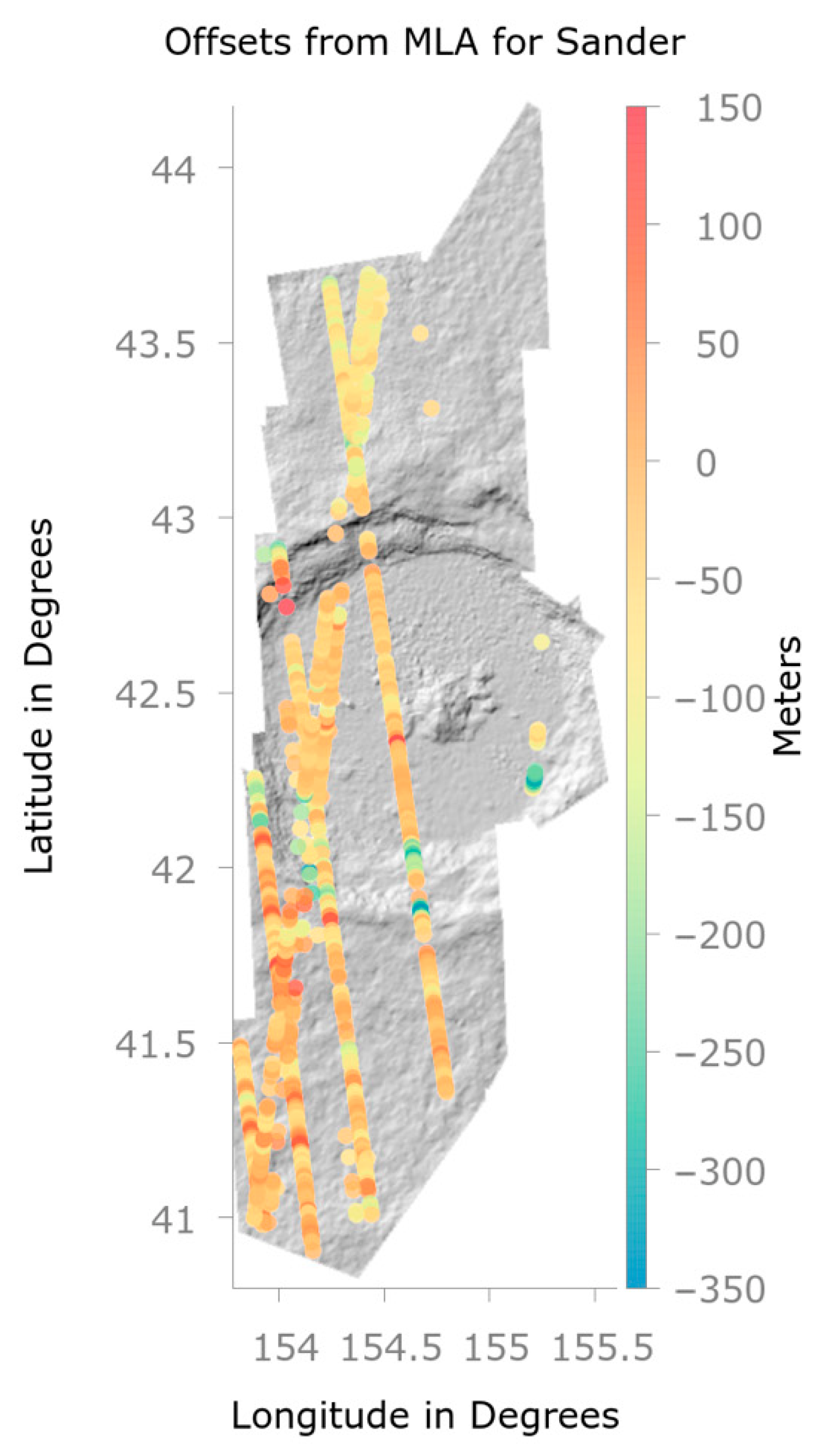
4.2. Offsets from MLA

Positional accuracy was evaluated by comparing DEM elevations with MLA elevations. Wherever MLA profiles directly crossed the DEM, the mean, median, and standard deviation of the offsets were evaluated (Figure 6). However, if, due to the highly elliptical orbit of MESSENGER and the sparse MLA coverage, no co-located profiles were available, then offsets were reported from the broader area WAC DEMs (controlled to MLA profiles). Some DEMs in the southern hemisphere had no MLA coverage; these products were not absolutely controlled, and for these we report only the relative precision.
With the range accuracy of MLA better than 20 m, ideally the measured differences between the DEMs and MLA profiles would also be <20 m. However, despite ongoing refinement of both our error analysis and DEM processing methods, consistently obtaining this level of accuracy remained challenging; manual alignment in stereo was made more difficult by varying image resolutions within stereo pairs. The seven DEMs we controlled to MLA had a median mean offset of −9 m. These offsets are also affected by horizontal errors due to uncertainty in position and orientation for MLA profiles [28]. Nevertheless, in all but one case, we were able to achieve mean offsets less than the pixel scale of the DEM (Table 3).

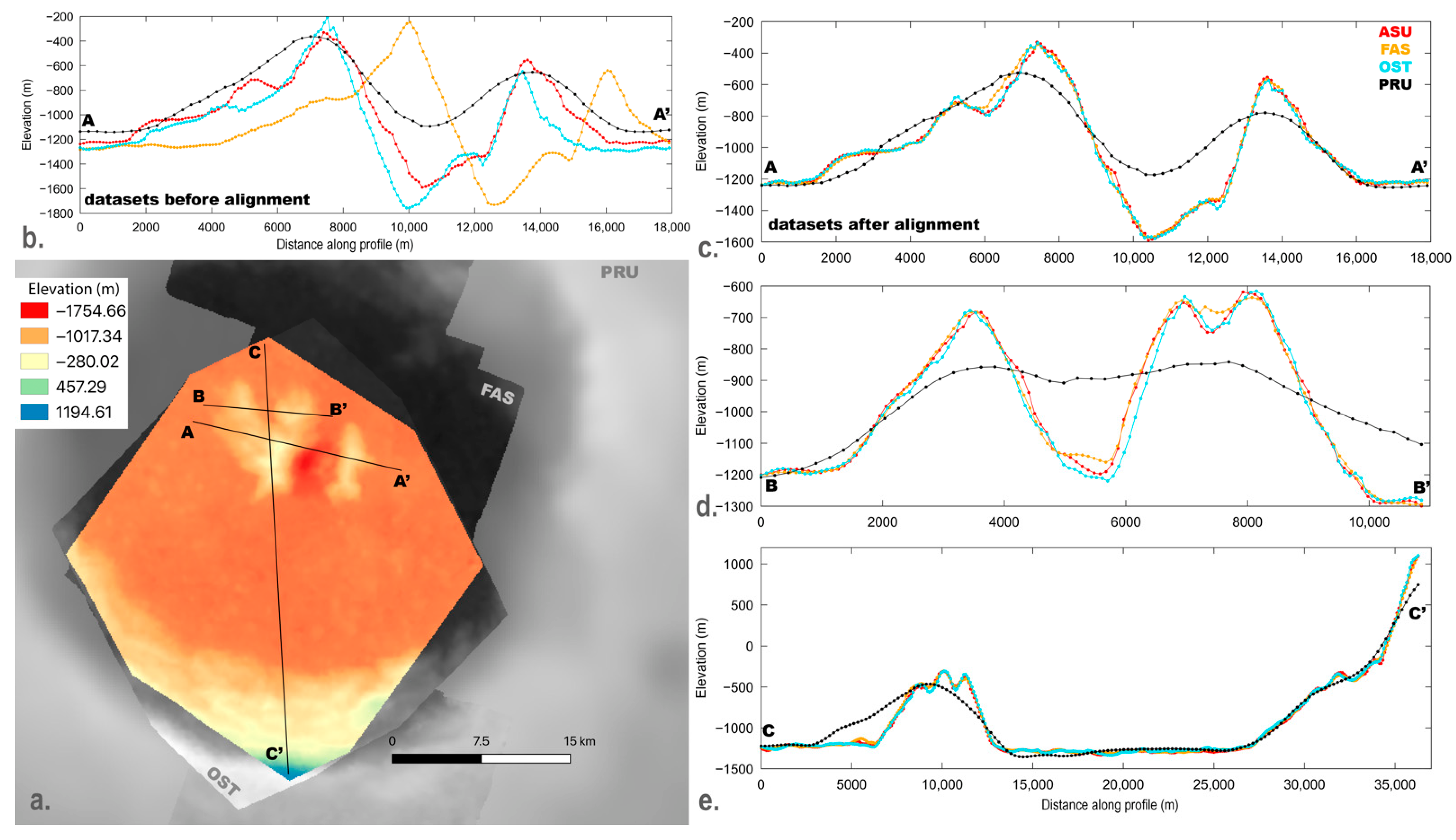
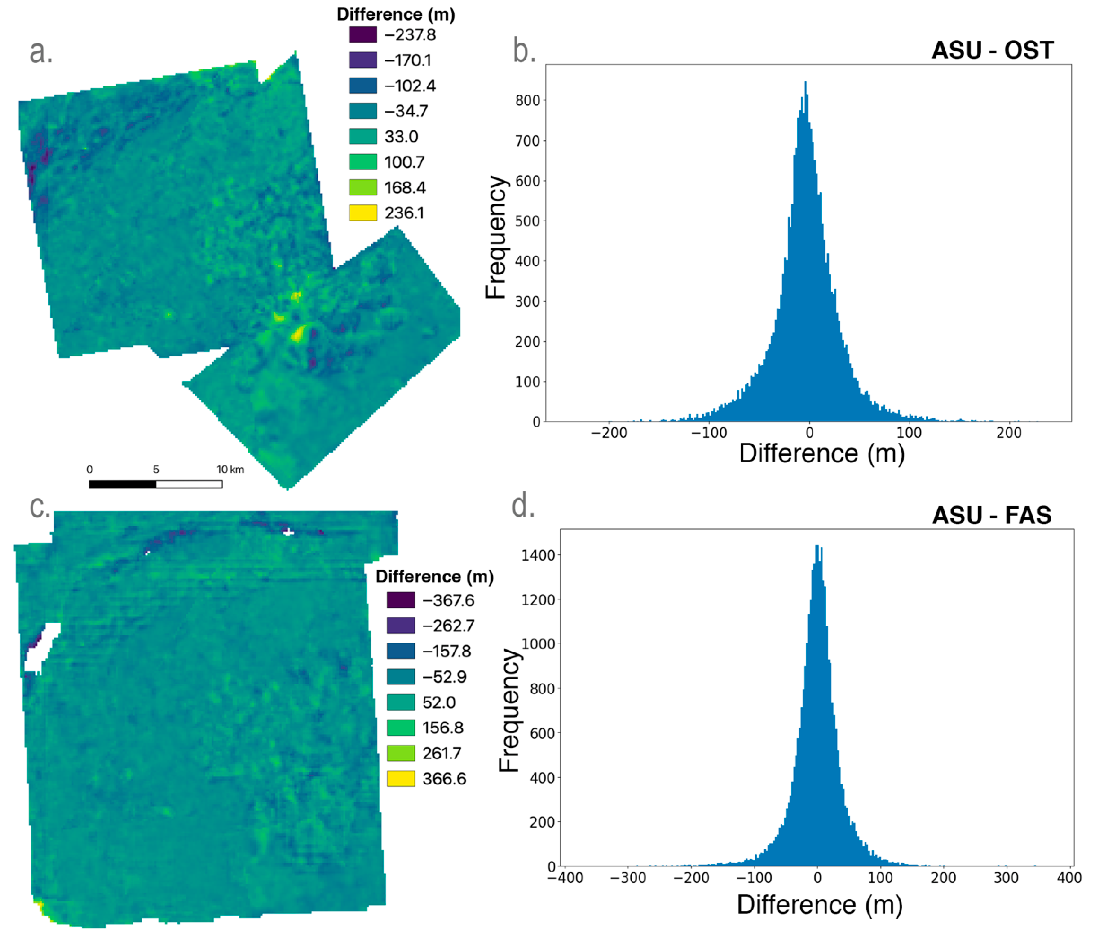
4.3. Comparison to Other Regional Topographic Products

The sparse MLA data does not allow us to fully evaluate the level of detail captured in the DEMs; therefore, we compared our products to overlapping DEMs from other publicly available regional datasets with overlapping DEMs and similar pixel scales (Table 4; Fassett [24]; Ostrach and Dundas [25]; and Preusker et al. [28]). Of the other high-resolution MDIS DEM datasets, we shared no overlapping DEMs with Tenthoff et al. [26], and Weirich et al.’s [27] DEMs are not yet publicly available.
Because the Ostrach and Dundas [25] (“OST”) and Fassett [24] (“FAS”) DEMs used reference radii of 2440.0 km, we added 600 m to these DEMs to adjust them to the 2439.4 km radii used by us (“ASU”) and by Preusker et al. [28] (“PRU”). The FAS and OST DEMs were also produced using version 2 (crossover-corrected) of the MLA profiles, whereas only version 1 of the MLA profiles was available when our DEMs were created. In the regions we examined, there was a km-scale shift between the two versions of the MLA. To account for any remaining offsets, we applied translations produced by running the pc_align tool from the Ames Stereo Pipeline [40].
To collect profiles for comparison, all the DEMs were loaded into QGIS [41]. The QGIS Profile Tool plugin was used to simultaneously collect profiles across the overlapping DEMs [42]. These profiles were then exported for analysis.
The translations from pc_align were predominantly horizontal (see Figure 7b,c). The horizontal offsets originate at least partially from differences between the two versions of MLA data used; other minor factors are the sparseness of the MLA profiles and the fact that each product was controlled to different profiles and numbers of MLA points.
The remaining differences between the DEMs are largely due to the differing pixel scales, as expected. The 222 m/px PRU DEMs are significantly smoother and shallower than the ASU (90–97 m) Degas DEMs when observing small features (e.g., the central peaks; Figure 7c,d), but elevation ranges agree well over longer baselines (e.g., crater diameter; Figure 7e). The detail captured by our Degas DEM most closely matches the detail from OST, which was produced using the same method. Minor differences between ASU and FAS likely originated from the different extraction algorithms, as well as some remaining misalignment.
Profiles over Sander crater’s central peak show that ASU, FAS, and OST DEMs capture similar features, but that the ASU mosaic, with approximately twice the pixel scale of FAS and OST, has more outliers and captures less fine detail (Figure 8). For the Sander site, we also viewed the DEMs as contour lines over an ASU DEM orthophoto (Figure 8b). For this small area, features in FAS are somewhat more smoothed out than in OST and ASU, while the ASU, as expected, contains more noise (see Figure 8c).
Our DEM of Kuiper crater was not controlled to MLA at all, as MLA becomes extremely sparse south of the equator. However, it does overlap with the PRU H06 quadrangle, which extends from 22.5°S to 22.5°N and therefore has MLA coverage over its northern half; its RMS vertical offset from MLA is 88 m [28]. We used pc_align to co-register the ASU Kuiper DEM to H06 and found a 934.4 m vertical offset, but a relatively good horizontal alignment (the optimal horizontal translation was <1 px for the ASU DEM) (Figure 9). At 270 m/px, the ASU DEM is a lower resolution than the 222 m/px quadrangle; however, more fine detail is captured in the ASU profile, likely due to differences in methodology and product coverage.
To more comprehensively evaluate the residual offsets between the DEMs, we created difference maps by subtracting the pc_aligned DEMs produced by FAS, OST, and PRU from the overlapping ASU DEMs. Table 5 shows the statistical summaries of these maps. The mean differences are within 4 m with the exception of three outliers; all are within 20 m. The means of the absolute differences are all less than 65 m. Larger mean absolute differences are associated with larger differences in pixel scales between the two DEMs. The standard deviations indicate fairly tight distributions; however, the minimums and maximums can be quite large, with total ranges between 285 m and 1226 m.
Following Bland et al., 2021 [43], we also created histograms of the difference maps to examine the distribution of offsets between the DEMs. They were approximately normally distributed, but with abnormally large tails. As a generally representative example, we show difference maps and histograms of Sander crater in Figure 10. Figure 10a,c show that the largest residual offsets are concentrated at the areas of most extreme topography: along the crater walls and at the steepest points of the central peak. Both FAS and OST here have an approximately 2× finer pixel scale than ASU, which may account for some of the residual offsets.
Our comparisons with other regional DEMs show that once large offsets are removed, products have comparable elevation ranges. Most discrepancies in the small-scale features captured are attributable to differences in DEM pixel scale, although minor horizontal misalignment and noise are also factors. The ASU, FAS, and OST DEMs, which have similar areas of coverage and numbers of input images, capture similar amounts of detail when they have roughly the same pixel scales.

5. Discussion: Scientific Application

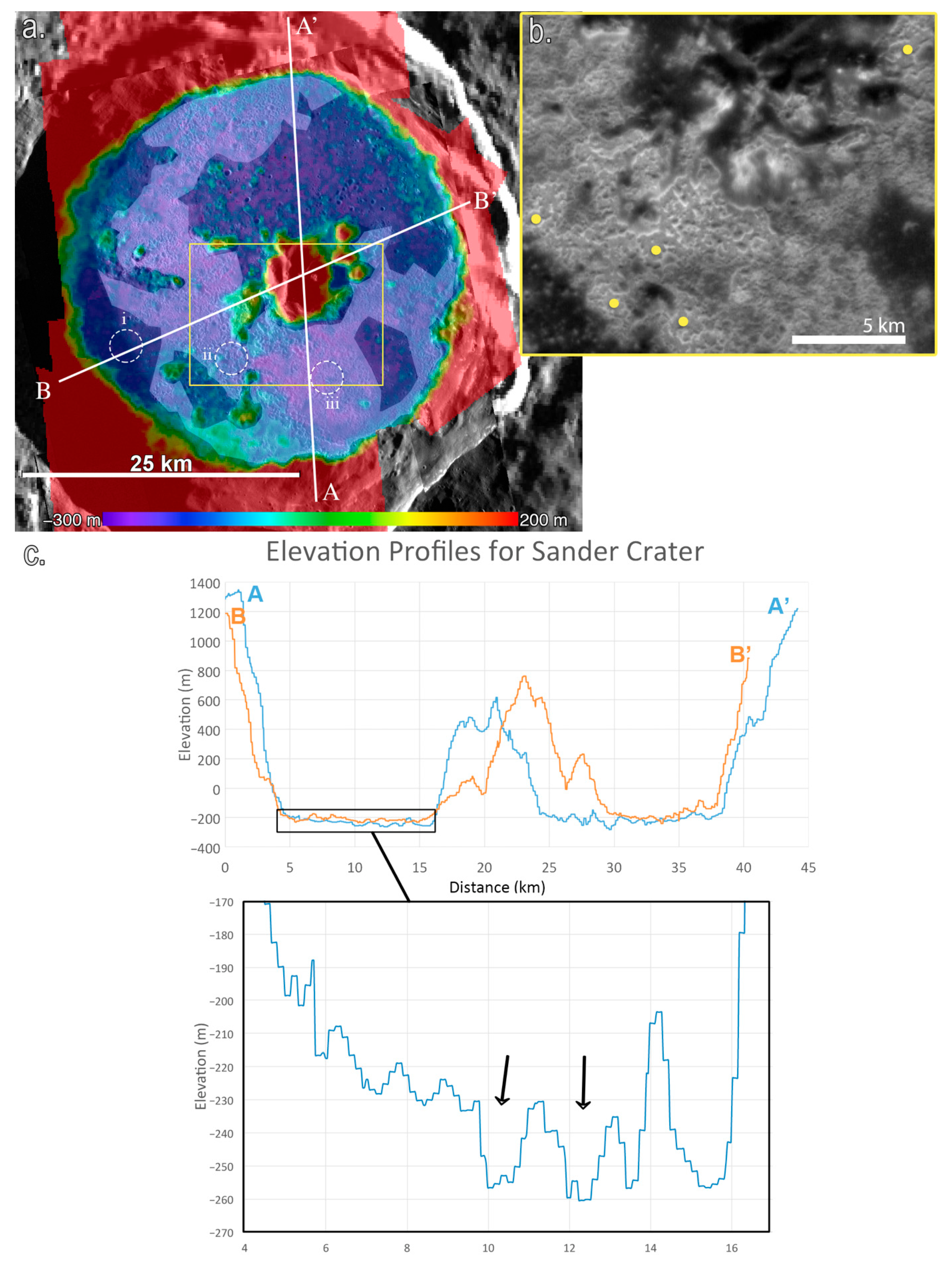
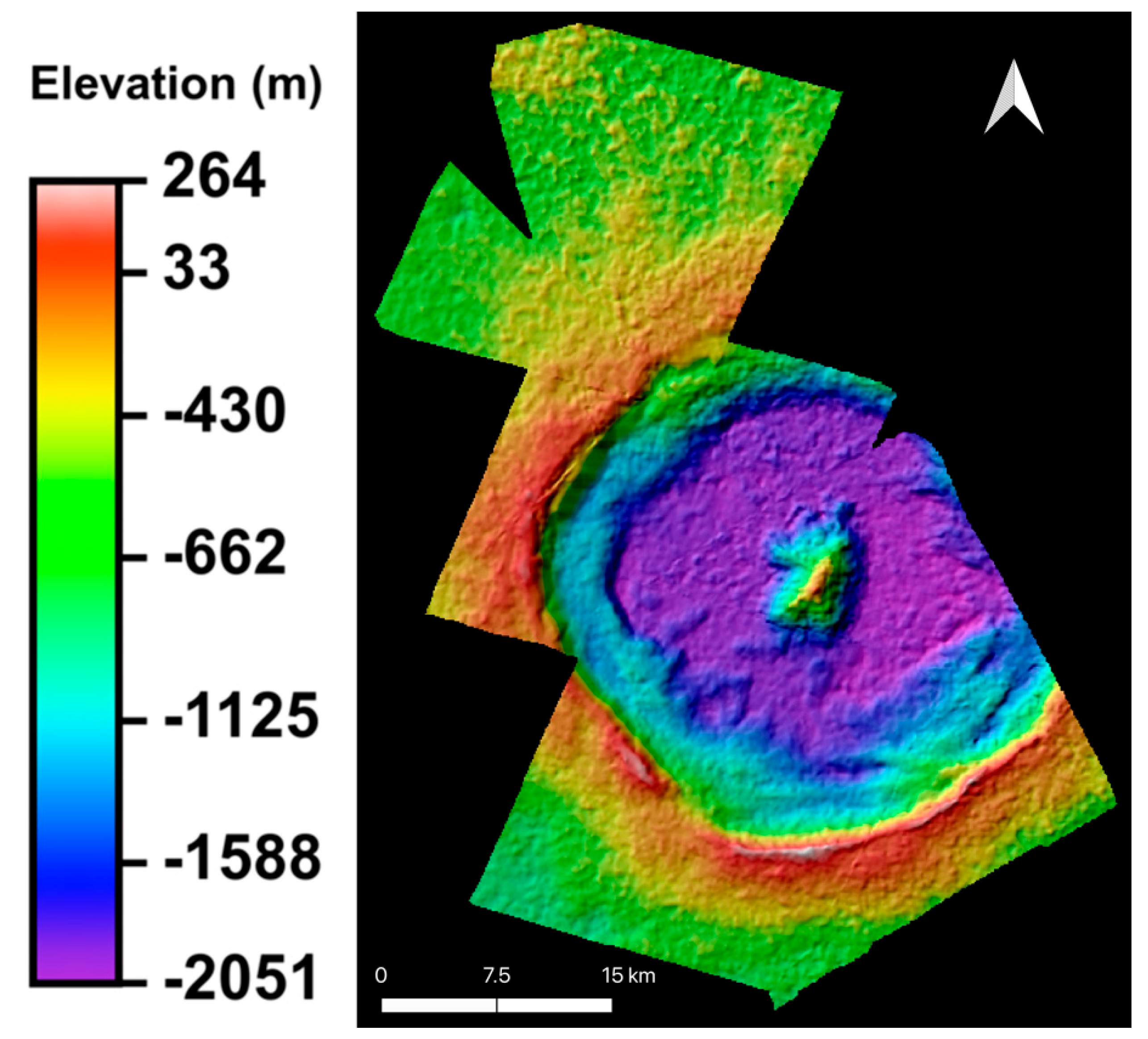
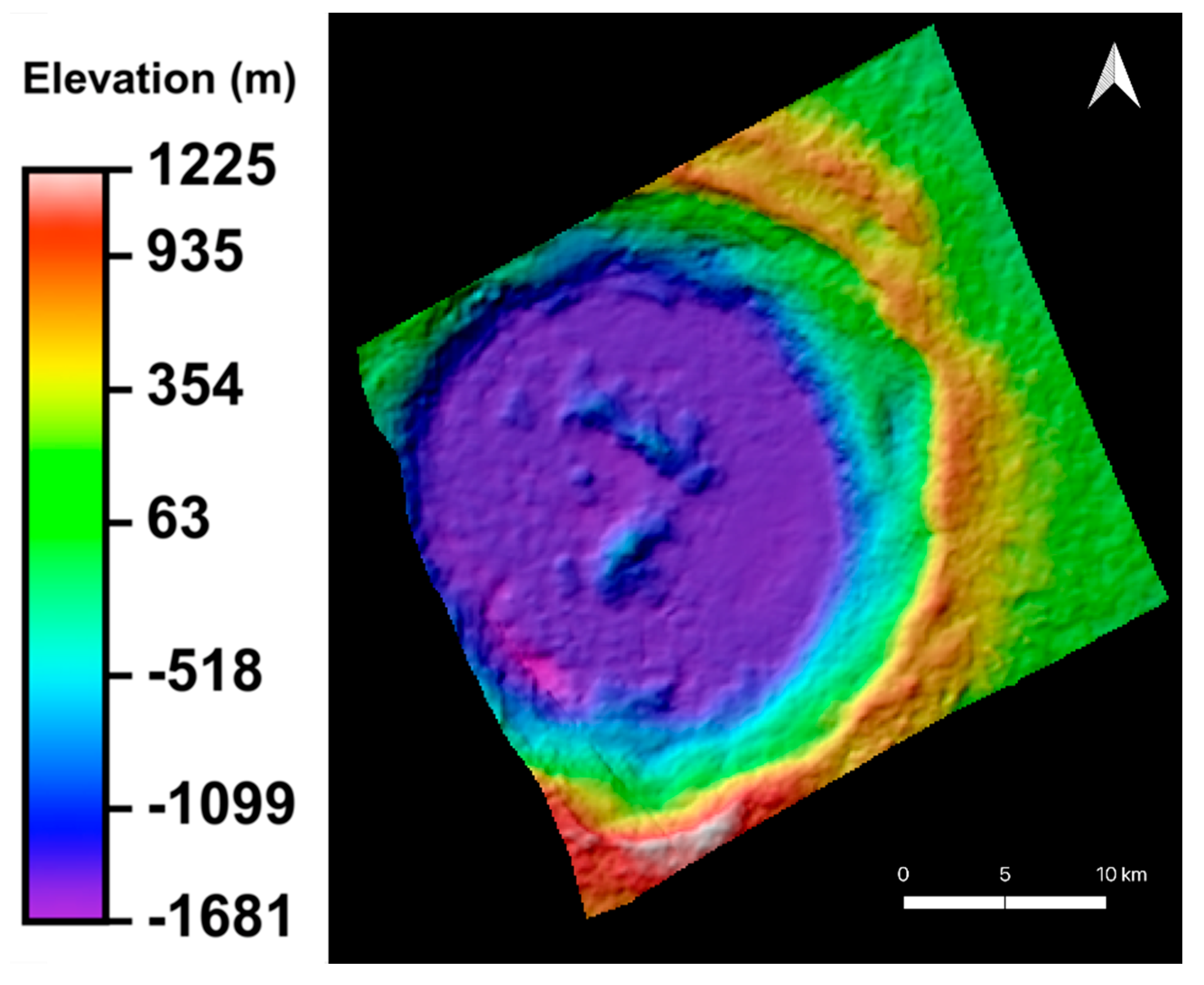
5.1. Anomalous High-Reflectance Regions in Kertész and Sander Craters

Blewett et al. [8,10,44,45] characterized distinctive features called “hollows” composed of relatively blue (433 nm to 559 nm ratio) and high-reflectance material. Hollows are shallow, rimless, irregularly shaped depressions, are distributed globally, and appear to form preferentially on crater floors, central peaks, and peak rings. The new DEMs of Sander crater, Kertész crater, and Raditladi basin presented here, all of which host hollows, provide the means to investigate formation theories proposed by previous studies.

5.2. Formation Hypotheses

Current hypotheses proposed to explain hollow formation agree that a volatile component is being lost, resulting in a collapse of the weakened matrix [10]. Several possibilities for the loss mechanism and the source of volatiles have been proposed. Vaughan et al. [46] suggested that sulfides or chlorides in differentiated impact melt could sublimate at surface temperatures. Blewett et al. [8,44] proposed that space weathering (sputtering by solar-wind ions, bombardment by micrometeoroids, exposure to solar heating, and ultraviolet fluxes) could cause the destruction and loss of volatile-bearing phases, such as sulfides. Alternately, Blewett et al. [8,44] noted that sequestered magmatic volatiles or fumarolic minerals from volcanic activity could later be exposed by impacts and lost by solar heating. Thomas et al. [9] suggested that endogenic heating of volatiles in upper crustal rocks could lead to sublimation. Phillips et al. [47] proposed a model in which thermal decay of sulfide minerals resulted in fumarolic systems that altered the near-surface and drove hollow formation. Measurements of hollow depths in high-resolution images have shown that hollows consistently have depths of tens of meters [8,9,24,45,46]. The mechanisms proposed generally posit that hollows grow in depth until either the material is exhausted or a lag deposit reaches sufficient thickness to halt the volatile loss [10].
For Kertész and Sander craters, we investigate three distinct floor units that are not observed in Raditladi: smooth sheet, pitted sheet, and bright knob/deep floor materials (Figure 11, Figure 12 and Figure 13). Vaughan et al. [46] defined these units and proposed that they represent the progression of hollow formation from smooth sheet to pitted sheet to the final stage, where the lowest elevation of the deep floor represents the maximum depth of the hollow-forming layer. Because the Kertész hollows are larger and more sharply defined than those in Sander crater, and the Kertész DEM, at 120 m/px, has a finer pixel scale than Sander (162 m/px) or Raditladi (180 m/px), we focused our investigation primarily on Kertész crater.

5.3. Findings: Kertész Crater

Kertész is a 33 km diameter crater with a depth of 2.2 km. It has two central peaks, with heights of 550 m and 600 m from the surrounding crater floor. A slump is present on the south wall, and abutting the crater wall on the southwest side of the floor just west of the slump is a pit ~360 m deeper than the surrounding crater floor. Hollows are distributed over the entire crater floor, extending in some areas to slumped units in the crater walls and onto lower regions of the central peaks (Figure 11).
In a sample of Kertész’s most well-defined hollows (six on the north/northwest side of the crater, four on the east/southeast sides; both regions defined by Vaughan et al. [46] as bright knob/deep floor), we calculated depth by subtracting minimum elevation on the hollow floor from the average hollow rim elevation. Measurements were taken in SOCET SET from the stereo pair released as KERTS01 using a stereo viewer (see Appendix C for red–blue anaglyphs of Kertész, Sander, and Raditladi stereo pairs). The images had pixel scales of 33 m and 40 m/px. The southeast hollows ranged from 20–62 m deep, while the significantly larger pits on the northwest side ranged from 35–101 m deep; the overall average depth was 51 m or a median depth of 48 m. Measurements taken from the DEM were somewhat shallower, averaging 30 m deep on the southeast side and 48 m deep on the northwest side. The stereo measurements, while involving a more ambiguous amount of uncertainty due to the user intervention required, are able to take advantage of the full resolution of the images; therefore, a stereo viewer may be required to extract the most data out of the stereo model. The depths found in stereo somewhat exceed the ~30 m maximum depth found by Vaughan et al. [46], possibly because that study used higher-resolution images and therefore was able to measure smaller hollows. The less well-defined hollows (“pitted sheet”) were too small to measure in our DEM, although both profiles and measurements taken in stereo in SOCET SET suggest depths of <10 m. Our measurements do fall within the general ranges of typical hollow depths found by previous studies (tens of meters).
Figure 11. (a) Kertész crater orthophoto overlaid with a color-shaded elevation map. Polygons show hollowed areas of floor investigated here; dotted circles mark characteristic units of pitted terrain (i), smooth floor (ii), and bright knob/deep floor (iii). Yellow dots indicate ten hollows measured for this study. See Appendix A for stereo pair details. (b) Elevation profiles. Inset profile shows a detail of bright knob/deep floor area; arrows indicate distinct hollows.
Remotesensing 14 03564 g011
We also noted several large contiguous regions where the Kertész smooth sheet was not pitted (or very minimally pitted), but was concave to at least the depth of the surrounding deep floor units; first, in a 4 km by 1 km sheet to the southwest, bordering the deep pit mentioned earlier; and secondly, in a smaller (1 × 1 km) region adjacent to the taller of the central peaks. At their highest points, these two smooth sheets are raised above the surrounding deep floor units to approximately the same height as the tops of the bright knobs, but they sink at their centers to depths of 27 m for the southwest sheet and 72 m for the central sheet. For the southwest sheet, the deepest point is approximately the same elevation as the bottom of the surrounding pits. For the central sheet, the lowest point of the concavity is at least 40 m lower than the average floor of the surrounding bright knob/deep floor unit. We discuss these smooth sheet regions in our analysis in Section 5.6.

5.4. Findings: Sander Crater

Sander crater is larger than Kertész, with a diameter of 52 km and a depth of 2.5 km. The floor of Sander crater is dominated by the unit designated as pitted sheet; these hollows are generally too small to be reliably measured at the DEM pixel scale (Figure 12). However, five distinct bright knob/deep floor hollows were identified and measured from the stereo pair used to create SANDR18. These hollows had an average depth of 31 m when measured in stereo (range of 9–65 m).
Figure 12. (a) Sander crater overlaid with a color-shaded elevation map. Polygons show hollowed areas of floor investigated here; dotted circles mark characteristic units of pitted terrain (i), smooth floor (ii), and bright knob/deep floor (iii). (b) Detail of SANDR18 orthophoto showing a portion of the crater floor and central peak. Yellow dots indicate the hollows measured for this study. See Appendix A for stereo pair details. (c) Elevation profiles. Inset profile shows a detail of bright knob/deep floor area; arrows indicate distinct hollows.
Remotesensing 14 03564 g012

5.5. Findings: Raditladi Basin

Hollows in Raditladi Basin surround the peak ring and are found on peak mountains (Figure 13). Unlike the hollows in Sander and Kertész, only one type of occurrence is found; the hollows are clearly defined and most closely resemble the bright knob/deep floor unit. However, the hollows are small enough (<1 km in diameter) that, in most cases, the DEM pixel scale (180 m/px) was not fine enough for precise measurements of individual hollows. Furthermore, the Raditladi DEM for the stereo pair measured (RADIT02) has a relative linear error of 137 m, significantly worse than either Kertész or Sander. We measured five of the largest hollows in stereo to find an average depth of 28 m (range of 24–32 m). This value differs from the average shadow-length depth for this area (44 m) reported by Blewett et al. [8]; however, our calculated depth likely represents a very conservative estimate due to the DEM’s coarser resolution.
Figure 13. (a) Hollows along the peak ring of Raditladi Basin in color-shaded elevation map overlaid on associated orthophoto mosaic. The white line (A–A’) indicates the extent of the profile taken across the hollowed region. Yellow dots indicate five individual hollows measured for this study. See Appendix A for stereo details. (b) Elevation profile.
Remotesensing 14 03564 g013

5.6. Analysis

Our results for the depth of the pitted regions, knobby regions, and individual hollows in Sander and Kertész are consistent with the depth of hollows found by other analyses. Blewett et al. [45] used shadow-length measurements on 565 high-resolution images to determine the depths of hollows and found an average depth of 24 m. Other shadow-length depth estimates of hollows [8,9,45,46] generally agree with the findings described here. Fassett [24] used MDIS DEMs produced with the Ames Stereo Pipeline to examine hollows and found an average depth of 32 m.
Blewett et al. [45] interpreted the typical depth of several tens of meters to indicate that hollows increase in depth until a sufficient lag deposit of devolatilized material develops and protects the underlying material from further loss of volatiles. Our observations of Kertész, Sander, and Raditladi are consistent with this hypothesis. The presence of a deep, smooth, concave sheet in Kertész crater is also consistent with Vaughan et al. [46]. They proposed that the hollows in Kertész formed in a massive sulfide or chloride deposit that resulted from differentiation and immiscibility in the impact melt that pooled in the crater floor. The concavities revealed by the topography may be related to volatile loss from such a thick, relatively pure volatile-bearing layer. Hollows found elsewhere commonly occur in places with steep topographic slopes (e.g., crater central peaks and walls) where pooling and differentiation of impact melt seems unlikely [10]. Thus, formation of hollows within impact melt pools (as at Kertész) may differ from that in material containing a lower abundance of a volatile-bearing phase.

6. Conclusions

Nine science sites consisting of 57 stereo pairs were completed (Appendix A; Appendix B) and archived to the NASA PDS in December 2016 as part of the MESSENGER DEM PDS Archive [29] (https://pdsimage2.wr.usgs.gov/archive/mess-h-mdis-5-dem-elevation-v1.0/MESSDEM_1001/DEM/REGIONAL/IMG/, accessed on 20 July 2022). Created from 49 NAC images, these DEMs are some of the highest-resolution, most precise, and most accurate topographic products of Mercury currently available. However, these represent only a few of the thousands of stereo pairs acquired with pixel scales of 13–150 m. As well as producing more DEMs, future work could include using global MESSENGER DEM products as additional sources of absolute control to improve local DEM accuracy and resolve issues with sparse MLA data at lower latitudes. We could also further automate several of the steps in our methodology (adding tie points, registering to MLA). That said, one of the benefits of our method over other, faster, more automated methods is that we use manual intervention and stereo viewing to visually inspect and validate the entire model [21,43]. More precise, accurate DEMs will provide necessary data for geologic studies of unique features on Mercury’s surface and complement observations by the SIMBIO-SYS instrument on the BepiColumbo spacecraft scheduled to enter orbit in 2025 [48].

Author Contributions

Conceptualization, M.S.R., M.R.H. and M.R.M.; methodology, M.R.H., M.R.M., S.S.S., M.C., K.J.B. and B.A.K.; software, K.J.B.; validation, M.R.H., M.R.M., S.S.S. and M.C.; formal analysis, M.R.M., M.R.H., H.R.K. and D.T.B.; investigation, H.R.K., B.A.K., M.R.M., M.R.H. and D.T.B.; resources, M.S.R. and K.J.B.; data curation, M.R.H. and M.R.M.; writing—original draft preparation, M.R.M., M.R.H. and H.R.K.; writing—review and editing, M.R.M., M.R.H., M.S.R., M.C., D.T.B., S.S.S. and K.J.B.; visualization, M.R.M., M.R.H. and H.R.K.; supervision, M.S.R.; project administration, M.S.R.; funding acquisition, M.S.R. All authors have read and agreed to the published version of the manuscript.

Funding

The majority of the work presented here was funded by NASA MESSENGER Project grant DTM3250022. The OSIRIS-REx Mission provided support for M. Chojnacki and S. Sutton. The contribution of D. Blewett was supported by NASA MESSENGER Participating Scientist grant NNX08AN29G.

Data Availability Statement

The MDIS NAC and WAC images, MLA data, and SPICE kernels used to produce the DEMs in this work are freely available through the MESSENGER PDS Archive at: http://pds-geosciences.wustl.edu/missions/messenger/index.htm (accessed on 20 July 2022). The DEMs themselves are archived in the PDS at https://0-doi-org.brum.beds.ac.uk/10.17189/1520282 (accessed on 20 July 2022).

Acknowledgments

We are deeply indebted to Annie Howington-Kraus, who shared with us the preliminary methodology, documentation, and pipelines for this work. We are grateful to Nick Aldana, Sarah Deitrick, Chris Hansen, Kerry Martin, and Corrine Rojas who worked to produce the products described here, and to Emerson Speyerer for his encouragement and thoughtful review.

Conflicts of Interest

The authors declare no conflict of interest. The funders had no role in the design of the study; in the collection, analyses, or interpretation of data; in the writing of the manuscript, or in the decision to publish the results.

Appendix A

List of DEMs created for each site and the images providing stereo for each DEM, DEM pixel scales, and relative linear errors. A DEM mosaic (indicated by a name ending in “MS”) was created for each site with more than one associated DEM.
SiteDEM NameImage 1Image 2Pixel Scale (m)Relative Linear Error (m)
Vent in Catullus CraterCATLS01EN1020925599MEN1020925715M8483.56
Cunningham CraterCNGHM01EN0215633679MEN1012716022M7848.97
‘‘CNGHM02EN0215633679MEN1012716026M7848.00
‘‘CNGHM03EN0215633673MEN1025248438M10553.67
‘‘CNGHM04EN0215633679MEN1025248438M10553.28
‘‘CNGHM05EN0215633673MEN1012716026M7848.51
‘‘CNGHM06EN0215633679MEN1025248434M10252.89
‘‘CNGHM07EN0215633685MEN1025248434M10252.64
‘‘CNGHM08EN1010038716MEN1012716018M7882.29
‘‘CNGHM09EN1010038716MEN1012716022M7884.69
‘‘CNGHMMS--10584.69
Degas CraterDEGAS01EN1008944217MEN1024240075M9769.26
Scarp in NW Rembrandt BasinHYNEK01EN1015859904MEN1015861167M500383.01
Kertész CraterKERTS01EN1010096377MEN1025335005M12071.46
‘‘KERTS02EN1010096377MEN1010096528M12097.34
‘‘KERTSMS--12097.34
Kuiper CraterKUIPR01EN0223659984MEN1002982634M270160.37
Paramour RupesPARMR01EN1045386684MEN1045387902M450256.82
‘‘PARMR02EN1045386684MEN1045387906M432256.94
‘‘PARMR03EN1045386688MEN1045387906M432260.93
‘‘PARMRMS--450260.93
Raditladi BasinRADIT01EN1015425730MEN1015426008M180134.99
‘‘RADIT02EN1015425734MEN1015426008M180136.62
‘‘RADIT03EN1015425734MEN1015426012M180134.74
‘‘RADITMS--180136.62
Sander CraterSANDR01EN1012745010MEN0218289182M10531.95
‘‘SANDR02EN1012745010MEN0218289189M10331.11
‘‘SANDR03EN1012745010MEN0217906385M16056.26
‘‘SANDR04EN1012745010MEN0233476482M9221.43
‘‘SANDR05EN1010125026MEN0217906385M16045.96
‘‘SANDR06EN1012745056MEN1010125151M8866.78
‘‘SANDR07EN1012745056MEN0218289182M10537.46
‘‘SANDR08EN1012745056MEN0218289189M10336.23
‘‘SANDR09EN1012745056MEN0217906385M16056.36
‘‘SANDR10EN1012745056MEN0233476482M9223.73
‘‘SANDR11EN1010125151MEN0217906385M16050.19
‘‘SANDR12EN1010125151MEN1010067392M8867.22
‘‘SANDR13EN1010125151MEN1010067396M8869.59
‘‘SANDR14EN0218289168MEN0217906381M16240.46
‘‘SANDR15EN0218289175MEN0217906381M16239.96
‘‘SANDR16EN0218289175MEN0217906385M16040.05
‘‘SANDR17EN0218289175MEN1012773887M10744.74
‘‘SANDR18EN0218289182MEN0217906385M16039.62
‘‘SANDR19EN0218289182MEN1012773893M10544.19
‘‘SANDR20EN0218289189MEN0217906385M16039.11
‘‘SANDR21EN0218289189MEN0217906389M15739.09
‘‘SANDR22EN0218289189MEN1012773893M10342.36
‘‘SANDR23EN0218289189MEN1012773899M10343.55
‘‘SANDR24EN0218289189MEN1012773904M10344.59
‘‘SANDR25EN0218289196MEN0217906389M15738.6
‘‘SANDR26EN0218289196MEN1012773904M10142.77
‘‘SANDR27EN0217906381MEN1012773887M16248.77
‘‘SANDR28EN0217906385MEN1010067392M16054.88
‘‘SANDR29EN0217906385MEN1012773887M16048.64
‘‘SANDR30EN0217906385MEN1012773893M16048.35
‘‘SANDR31EN0233476482MEN1012773887M9225.61
‘‘SANDR32EN0233476482MEN1012773893M9226.36
‘‘SANDR33EN0233476482MEN1012773899M9227.14
‘‘SANDR34EN0233476487MEN1012773899M9126.22
‘‘SANDR35EN0233476487MEN1012773904M9126.99
‘‘SANDR36EN0233476492MEN1012773904M9026.11
‘‘SANDRMS--16269.59

Appendix B

Color-shaded relief maps of all completed regional MESSENGER DEMs (nine sites).
Figure A1. Vent in Catullus Crater.
Remotesensing 14 03564 g0a1
Figure A2. Cunningham Crater.
Remotesensing 14 03564 g0a2
Figure A3. Degas Crater.
Remotesensing 14 03564 g0a3
Figure A4. Scarp in northwest Rembrandt Basin.
Remotesensing 14 03564 g0a4
Figure A5. Kertész Crater.
Remotesensing 14 03564 g0a5
Figure A6. Kuiper Crater.
Remotesensing 14 03564 g0a6
Figure A7. Paramour Rupes.
Remotesensing 14 03564 g0a7
Figure A8. Hollows in Raditladi Basin.
Remotesensing 14 03564 g0a8
Figure A9. Sander Crater.
Remotesensing 14 03564 g0a9

Appendix C

Anaglyphs of DEMs containing hollowed regions. Note that anaglyphs are vertically exaggerated by approximately 10× the true vertical distance.
Figure A10. Kertész Crater. Images: EN1010096377M, EN1010096528M.
Remotesensing 14 03564 g0a10
Figure A11. Sander Crater. Images: EN0218289182M, EN0217906385M.
Remotesensing 14 03564 g0a11
Figure A12. Raditladi Basin. Images: EN1015426008M, EN1015425734M.
Remotesensing 14 03564 g0a12

References

  1. Hawkins, S.E., III; Boldt, J.D.; Darlington, E.H.; Espiritu, R.; Gold, R.E.; Gotwols, B.; Grey, M.P.; Hash, C.D.; Hayes, J.R.; Jaskulek, S.E.; et al. The Mercury Dual Imaging System on the MESSENGER Spacecraft. Space Sci. Rev. 2007, 131, 247–338. [Google Scholar] [CrossRef]
  2. Hawkins, S.E., III; Murchie, S.L.; Becker, K.J.; Selby, C.M.; Turner, F.S.; Noble, M.W.; Chabot, N.L.; Choo, T.H.; Darlington, E.H.; Denevi, B.W.; et al. In-flight performance of MESSENGER’s Mercury Dual Imaging System. SPIE Opt. Eng. Appl. 2009, 7441, 74410Z. [Google Scholar] [CrossRef]
  3. Chabot, N.L.; Denevi, B.W.; Murchie, S.L.; Hash, C.D.; Ernst, C.M.; Blewett, D.T.; Nair, H.; Laslo, N.R.; Solomon, S.C. Mapping Mercury: Global imaging strategy and products from the MESSENGER mission. In Proceedings of the 47th Annual Lunar and Planetary Science Conference, The Woodlands, TX, USA, 21–25 May 2016. Abstract #1256. [Google Scholar]
  4. Moessner, D.P.; McAdams, J.V. Design, implementation, and outcome of MESSENGER’s trajectory from launch to impact. In Proceedings of the Astrodynamics Specialist Conference, American Astronautical Society (AAS 15-608), Vail, CO, USA, 9–13 August 2015. [Google Scholar]
  5. Sun, X.; Neumann, G.A. Calibration of the Mercury Laser Altimeter on the MESSENGER Spacecraft. IEEE Trans. Geosci. Remote Sens. 2015, 53, 2860–2874. [Google Scholar] [CrossRef]
  6. Solomon, S.C.; Anderson, B.J. The MESSENGER Mission: Science and Implementation Overview. In Mercury: The View after MESSENGER; Cambridge University Press: Cambridge, UK, 2018; pp. 1–29. [Google Scholar] [CrossRef]
  7. Bedini, P.D.; Solomon, S.C.; Finnegan, E.J.; Calloway, A.B.; Ensor, S.L.; McNutt, R.L.; Anderson, B.J.; Prockter, L.M. MESSENGER at Mercury: A mid-term report. Acta Astronaut. 2012, 81, 369–379. [Google Scholar] [CrossRef]
  8. Blewett, D.T.; Chabot, N.L.; Denevi, B.W.; Ernst, C.M.; Head, J.W.; Izenberg, N.R.; Murchie, S.L.; Solomon, S.C.; Nittler, L.R.; McCoy, T.J.; et al. Hollows on Mercury: MESSENGER Evidence for Geologically Recent Volatile-Related Activity. Science 2011, 333, 1856–1859. [Google Scholar] [CrossRef] [Green Version]
  9. Thomas, R.J.; Rothery, D.A.; Conway, S.J.; Anand, M. Hollows on Mercury: Materials and mechanisms involved in their formation. Icarus 2014, 229, 221–235. [Google Scholar] [CrossRef] [Green Version]
  10. Blewett, D.T.; Ernst, C.M.; Murchie, S.L.; Vilas, F. Mercury’s Hollows. In Mercury: The View after MESSENGER; Cambridge University Press: Cambridge, UK, 2018; pp. 324–345. [Google Scholar] [CrossRef]
  11. Cavanaugh, J.F.; Smith, J.C.; Sun, X.; Bartels, A.E.; Ramos-Izquierdo, L.; Krebs, D.J.; McGarry, J.F.; Trunzo, R.; Novo-Gradac, A.M.; Britt, J.L.; et al. The Mercury Laser Altimeter Instrument for the MESSENGER Mission. Space Sci. Rev. 2007, 131, 451–479. [Google Scholar] [CrossRef] [Green Version]
  12. Solomon, S.C.; McNutt, R.L.; Gold, R.E.; Domingue, D.L. MESSENGER Mission Overview. Space Sci. Rev. 2007, 131, 3–39. [Google Scholar] [CrossRef]
  13. MESSENGER MLA Team. MESSENGER MLA Calibrated (CDR/RDR) Data Bundle, Version 1. 2018. Available online: https://0-doi-org.brum.beds.ac.uk/10.17189/1518580 (accessed on 20 July 2022).
  14. Zuber, M.T.; Smith, D.E.; Phillips, R.J.; Solomon, S.C.; Neumann, G.A.; Hauck, S.A., II; Peale, S.J.; Barnouin, O.S.; Head, J.W.; Johnson, C.L.; et al. Topography of the Northern Hemisphere of Mercury from MESSENGER Laser Altimetry. Science 2012, 336, 217–220. [Google Scholar] [CrossRef] [Green Version]
  15. MESSENGER MLA Team. MESSENGER MLA CDR/RDR Data Set Description, Version 1. Lidvid urn:nasa:pds:mess_mla_calibrated:document:mess_mla_cdr_rdr_ds::1.0. 2018. Available online: https://pds-geosciences.wustl.edu/messenger/mess-e_v_h-mla-3_4-cdr_rdr-data-v1/messmla_2001/document/mess_mla_cdr_rdr_ds.txt (accessed on 14 July 2022).
  16. Anderson, J.A.; Sides, S.C.; Soltesz, D.L.; Sucharski, T.L.; Becker, K.J. Modernization of the Integrated Software for Imagers and Spectrometers. In Proceedings of the 35th Lunar and Planetary Science Conference, Houston, TX, USA, 15 March 2004. Abstract #2039. [Google Scholar]
  17. Keszthelyi, L.; Becker, T.; Sides, S.; Barrett, J.; Cook, D.; Lambright, S.; Lee, E.; Milazzo, M.; Oyama, K.; Richie, J.; et al. Support and future vision for the Integrated Software for Imagers and Spectrometers. In Proceedings of the 44th Lunar and Planetary Science Conference, The Woodlands, TX, USA, 6–8 March 2013. Abstract #2546. [Google Scholar]
  18. Adoram-Kershner, L.; Berry, K.; Lee, K.; Laura, J.; Mapel, J.; Paquette, A.; Rodriguez, K.; Sanders, A.; Sides, S.; Weller, L.; et al. USGS Astrogeology/ISIS3: ISIS3.10.1 Public Release. 2020. Available online: https://zenodo.org/record/3697255 (accessed on 20 July 2022).
  19. Miller, S.B.; Walker, A.S. Further developments of Leica digital photogrammetric systems by Helava. ACSM/ASPRS Annu. Conv. Expo. 1993, 3, 256–263. [Google Scholar]
  20. Miller, S.B.; Walker, A.S. Die Entwicklung der digitalen photogrammetrischen Systeme von Leica und Helava. Z. Photogramm. Fernerkund. 1995, 63, 4–16. [Google Scholar]
  21. Henriksen, M.R.; Manheim, M.R.; Burns, K.N.; Seymour, P.; Speyerer, E.J.; Deran, A.; Boyd, A.K.; Howington-Kraus, E.; Rosiek, M.R.; Archinal, B.A.; et al. Extracting accurate and precise topography from LROC Narrow Angle Camera stereo observations. Icarus 2017, 283, 122–137. [Google Scholar] [CrossRef]
  22. Kirk, R.L.; Howington-Kraus, E.; Rosiek, M.R.; Anderson, J.A.; Archinal, B.A.; Becker, K.J.; Cook, D.A.; Galuszka, D.M.; Geissler, P.E.; Hare, T.; et al. Ultrahigh resolution topographic mapping of Mars with MRO HiRISE stereo images: Meter-scale slopes of candidate Phoenix landing sites. J. Geophys. Res. Planets 2008, 113. [Google Scholar] [CrossRef]
  23. Sutton, S.S.; Chojnacki, M.; McEwen, A.S.; Kirk, R.L.; Dundas, C.M.; Schaefer, E.I.; Conway, S.J.; Diniega, S.; Portyankina, G.; Landis, M.E.; et al. Revealing Active Mars with HiRISE Digital Terrain Models. Remote Sens. 2022, 14, 2403. [Google Scholar] [CrossRef]
  24. Fassett, C.I. Ames stereo pipeline-derived digital terrain models of Mercury from MESSENGER stereo imaging. Planet. Space Sci. 2016, 134, 19–28. [Google Scholar] [CrossRef] [Green Version]
  25. Ostrach, L.R.; Dundas, C.M. Topographic assessment of hollows on Mercury: Distinguishing among formation hypotheses. In Proceedings of the Lunar and Planetary Science Conference XLVIII, The Woodlands, TX, USA, 20–24 March 2017. Abstract #1656. [Google Scholar]
  26. Tenthoff, M.; Wohlfarth, K.; Wöhler, C. High Resolution Digital Terrain Models of Mercury. Remote Sens. 2020, 12, 3989. [Google Scholar] [CrossRef]
  27. Weirich, J.R.; Domingue, D.L.; Palmer, E.E.; Rodriguez, A. High-Resolution Topography and Photometric Data Cubes for Mercury and the Moon. In Proceedings of the Lunar and Planetary Science Conference LIII, The Woodlands, TX, USA, 7–11 March 2022. Abstract #1115. [Google Scholar]
  28. Preusker, F.; Stark, A.; Oberst, J.; Matz, K.-D.; Gwinner, K.; Roatsch, T.; Watters, T.R. Toward high-resolution global topography of Mercury from MESSENGER orbital stereo imaging: A prototype model for the H6 (Kuiper) quadrangle. Planet. Space Sci. 2017, 142, 26–37. [Google Scholar] [CrossRef] [Green Version]
  29. Becker, K.; Robinson, M.; Pruesker, F. MESSENGER MDIS DEM V1.0, NASA Planetary Data System. 2015. Available online: https://0-doi-org.brum.beds.ac.uk/10.17189/1520282 (accessed on 20 July 2022).
  30. Becker, K.J.; Archinal, B.A.; Hare, T.H.; Kirk, R.L.; Howington-Kraus, E.; Robinson, M.S.; Rosiek, M.R. Criteria for automated identification of stereo image pairs. In Proceedings of the Lunar and Planetary Science Conference XLVI, The Woodlands, TX, USA, 16–20 March 2015. Abstract #2703. [Google Scholar]
  31. McAdams, J.V.; Bryan, C.G.; Bushman, S.S.; Calloway, A.B.; Carranza, E.; Flanigan, S.H.; Kirk, M.N.; Korth, H.; Moessner, D.P.; O’Shaughnessy, D.J.; et al. Engineering MESSENGER’s grand finale at Mercury—The low-altitude hover campaign. In Proceedings of the Astrodynamics Specialist Conference, American Astronautical Society (AAS 15-634), Vail, CO, USA, 9–11 August 2015. [Google Scholar]
  32. Becker, K.J.; Edmundson, K.; Weller, L.; Isbell, C.; Bowman-Cisneros, E.; Speyerer, E.; Henriksen, M.; Preusker, F.; Ensor, S.; Reid, M.; et al. MESSENGER Digital Elevation Model Software Interface Specification, Version 1.6. 2017. Available online: https://pdsimage2.wr.usgs.gov/archive/mess-h-mdis-5-dem-elevation-v1.0/MESSDEM_1001/DOCUMENT/MSGR_DEM_SIS.PDF (accessed on 20 July 2022).
  33. Forstner, W.; Wrobel, B.; Paderes, F.; Fraser, C.S.; Dolloff, J.; Mikhail, E.M.; Rujikietgumjorn, W. Analytical photogrammetric operations. In Manual of Photogrammetry, 6th ed.; McGlone, J.C., Ed.; American Society for Photogrammetry and Remote Sensing: Bethesda, MD, USA, 2013; pp. 785–955. [Google Scholar]
  34. BAE Systems. SOCET SET User’s Manual; Version 5.6; BAE Systems. 2011. Available online: https://www.geospatialexploitationproducts.com/content/ (accessed on 20 July 2022).
  35. BAE Systems. Next-Generation Automatic Terrain Extraction (NGATE). White Paper. 2007. Available online: https://www.geospatialexploitationproducts.com/wp-content/uploads/2016/01/wp_ngate.pdf (accessed on 20 July 2022).
  36. Zhang, B. Towards a higher level automation in softcopy photogrammetry: NGATE and LIDAR processing in SOCET SET. In Proceedings of the GeoCue Corporation 2nd Annual Technical Exchange Conference, Nashville, TN, USA, 26–27 September 2006. [Google Scholar]
  37. Miller, S. Photogrammetric products. In Manual of Photogrammetry, 6th ed.; McGlone, J.C., Ed.; American Society for Photogrammetry and Remote Sensing: Bethesda, MD, USA, 2013; pp. 1009–1043. [Google Scholar]
  38. Warmerdam, F. The Geospatial Data Abstraction Library. In Open Source Approaches in Spatial Data Handling; Hall, G.B., Leahy, M.G., Eds.; Springer: Berlin/Heidelberg, Germany, 2008; pp. 87–104. [Google Scholar] [CrossRef]
  39. Burns, K.N.; Speyerer, E.J.; Robinson, M.S.; Tran, T.; Rosiek, M.R.; Archinal, B.A.; Howington-Kraus, E.; the LROC Science Team. Digital Elevation Models and Derived Products from LROC NAC stereo observations. ISPRS Int. Arch. Photogramm. Remote Sens. Spat. Inf. Sci. 2012, 39, 483–488. [Google Scholar] [CrossRef] [Green Version]
  40. Beyer, R.A.; Alexandrov, O.; McMichael, S. The Ames Stereo Pipeline: NASA’s Open Source Software for Deriving and Processing Terrain Data. Earth Space Sci. 2018, 5, 537–548. [Google Scholar] [CrossRef]
  41. QGIS.org. QGIS Geographic Information System. QGIS Association. 2022. Available online: http://www.qgis.org (accessed on 6 June 2022).
  42. Jurgiel, B.; Verchere, P.; Tourigny, E.; Becerra, J. Profile Tool, v4.1.7. PANOimagen S. L. Available online: https://github.com/PANOimagen/profiletool (accessed on 20 July 2022).
  43. Bland, M.T.; Kirk, R.L.; Galuszka, D.M.; Mayer, D.P.; Beyer, R.A.; Fergason, R.L. How Well Do We Know Europa’s Topography? An Evaluation of the Variability in Digital Terrain Models of Europa. Remote Sens. 2021, 13, 5097. [Google Scholar] [CrossRef]
  44. Blewett, D.T.; Vaughan, W.M.; Xiao, Z.; Chabot, N.L.; Denevi, B.W.; Ernst, C.M.; Helbert, J.; D’Amore, M.; Maturilli, A.; Head, J.W.; et al. Mercury’s hollows: Constraints on formation and composition from analysis of geological setting and spectral reflectance. J. Geophys. Res. Planets 2013, 118, 1013–1032. [Google Scholar] [CrossRef] [Green Version]
  45. Blewett, D.T.; Stadermann, A.C.; Susorney, H.C.; Ernst, C.M.; Xiao, Z.; Chabot, N.L.; Denevi, B.W.; Murchie, S.L.; McCubbin, F.M.; Kinczyk, M.J.; et al. Analysis of MESSENGER high-resolution images of Mercury’s hollows and implications for hollow formation. J. Geophys. Res. Planets 2016, 121, 1798–1813. [Google Scholar] [CrossRef]
  46. Vaughan, W.M.; Helbert, J.; Blewett, D.T.; Head, J.W.; Murchie, S.L.; Gwinner, K.; McCoy, T.J.; Solomon, S.C. Hollow-forming layers in impact craters on Mercury: Massive sulfide or chloride deposits formed by impact melt differentiation? In Proceedings of the Lunar and Planetary Science Conference XLIII, The Woodlands, TX, USA, 7–11 March 2022. Abstract #1187. [Google Scholar]
  47. Phillips, M.S.; Moersch, J.E.; Viviano, C.E.; Emery, J.P. The lifecycle of hollows on Mercury: An evaluation of candidate volatile phases and a novel model of formation. Icarus 2021, 359, 114306. [Google Scholar] [CrossRef]
  48. Benkhoff, J.; Murakami, G.; Baumjohann, W.; Besse, S.; Bunce, E.; Casale, M.; Cremosese, G.; Glassmeier, K.-H.; Hayakawa, H.; Heyner, D.; et al. BepiColombo—Mission Overview and Science Goals. Space Sci. Rev. 2021, 217, 90. [Google Scholar] [CrossRef]
Figure 1. Workflow diagram for processing MESSENGER high-resolution stereo pairs to DEMs (adapted from Henriksen et al. [21]).
Remotesensing 14 03564 g001
Figure 2. Criteria for choosing NAC and WAC images to produce stereo pairs (blue indicates optimal conditions, yellow is acceptable, and red is not serviceable). The values shown here are adapted from Becker et al. [30].
Remotesensing 14 03564 g002
Figure 3. Stereo pairs used to create the Sander crater DEM mosaic: (A) shows the footprints of the 21 images chosen, while (B) shows the footprints of the 36 individual DEMs made from those images.
Remotesensing 14 03564 g003
Figure 4. Tie points connecting Kertész NAC DEM (top; displayed as a color-shaded relief map) to an overlapping WAC DEM (middle; made from image pair EW0218288557G, EW0233348623G), which is controlled to MLA profiles (bottom) projected to Mercury’s surface. Black circles represent tie points between the NAC and WAC images, while black squares represent control points in the WAC DEM from MLA points.
Remotesensing 14 03564 g004
Figure 5. PDS and derived products from the Sander crater DEM mosaic (42.42°N, 154.64°E), created from 21 images forming 36 stereo pairs. The DEM mosaic, orthophoto mosaics at two resolutions, and a confidence map are available in PDS format, as well as individual DEMs, four orthophotos, and confidence maps for each stereo pair. In addition, terrain-shaded relief, color-shaded relief, and slope maps are derived from each DEM and are released as 8-bit GeoTIFFs along with a 32-bit GeoTIFF of the DEM. See Appendix A for stereo pair details.
Remotesensing 14 03564 g005
Figure 6. Plot showing the difference between MLA profiles and the Sander crater regional DEM. The DEM mosaic consists of 36 stereo pairs with a pixel scale of 162 m.
Remotesensing 14 03564 g006
Figure 7. Degas crater profiles. (a) Colorized elevation map of ASU (97 m/px) shown over OST DEM (90 m/px), FAS DEM (95 m/px), and PRU H03 quadrangle (222 m/px). (b) Elevations for profile A for each DEM before alignment. (c) Elevations for profile A after alignment. (d,e) Post-alignment elevations for profiles B and C.
Remotesensing 14 03564 g007
Figure 8. Sander crater topographic profiles. (a) Colorized elevation map of ASU (SANDRMS; 162 m/px). Gray polygons show the extents of FAS (90 m/px) and OST (80 m/px); both have been aligned to ASU. (b) ASU, FAS, and OST displayed as 30 m contours overlaid on an ASU orthophoto. (ce) DEM elevations for profiles A, B, and C.
Remotesensing 14 03564 g008
Figure 9. Kuiper crater profiles. Here, ASU DEM has been vertically translated by subtracting 934.4 m; no other alignment was performed. (a) ASU 90 m contour map overlaid on ASU orthophoto, shown over PRU DEM. (b) Elevations from ASU (270 m/px) and PRU (222 m/px) for profile A.
Remotesensing 14 03564 g009
Figure 10. (a,c) Difference maps of Sander crater: OST and FAS DEMs subtracted from ASU DEM. (b,d) Histograms of the difference values.
Remotesensing 14 03564 g010
Table 1. Image selection criteria statistics for the stereo images used in this study.
Acquisition ConditionsIdentifying Stereo Pairs
Incidence Angle (°)Emission Angle (°)Overlap PercentagePixel Scale RatioStrength of StereoShadow Tip Distance (°)Solar Az. Angle Diff. (°)
Minimum3010.450.400.370.000.00
Maximum64501000.991.390.0232.65
Average452656.860.660.800.158.99
Median443251.810.680.720.116.60
Table 2. A priori bundle adjustment parameters.
MST ParametersValues
Camera ΔX100 m
Camera ΔY100 m
Camera ΔZ10 m
Attitude ΔOmega *0.1°
Attitude Δphi *0.1°
Attitude Δkappa *0.1°
* These three attitude parameters are functionally similar to roll, pitch, and yaw, although not exactly the same. Roll, pitch, and yaw describe the rotation of a body while phi, omega, and kappa describe the rotation of an image relative to a projected coordinate system.
Table 3. Summary data and error analysis for completed regions.
Site Name# of Stereo PairsCenter Latitude, Longitude
(°N, °E)
DEM Mosaic Pixel Scale (m)Relative Linear (Vertical)
Error (m)
# of MLA Points for ComparisonMLA Mean (Vertical) Offset (m)MLA Standard Deviation (m)
Catullus Crater *121.88°, 292.5°8484777−255188
Cunningham Crater930.40°, 157.0°10585127258
Degas Crater136.86°, 232.6°9770125−1109
Scarp in NW Rembrandt Basin1−31.16°, 82.5°500383---
Kertész Crater231.45°, 146.3°1209827−951
Kuiper Crater1−11.3°, 329.1°270161---
Paramour Rupes *3−5.07°, 145.1°450261138−5185
Raditladi Hollows315.20°, 120.2°180137154−4452
Sander Crater3642.50°, 154.7°16270756−4465
* MLA offsets are obtained from WAC DEMs tied to the NAC DEMs.
Table 4. Regional MDIS DEM datasets used in this comparison.
DatasetMethodResolution Range (m/px)Number of DEMsASU Site (# DEMs from Dataset That Overlap)
Manheim et al. (this study) (“ASU”)SOCET SET78–5009 mosaics; 57 individual DEMs-
Fassett [24] (“FAS”)Ames Stereo Pipeline45–24596Catullus (2), Degas (1), Raditladi (3), Sander (1)
Ostrach and Dundas [25] (“OST”)SOCET SET25–12011Degas (1), Sander (1), Kertész (2)
Preusker et al. [28] (“PRU”)Custom stereophotogrammetry2224 quadranglesCatullus (1), Degas (1), Kuiper (1)
Table 5. Summary of differences between ASU DEMs and overlying DEMs.
ASU DEMSubtracted DEMStandard DeviationMean Diff. (m)Std Dev. of Abs. Diff.Mean Abs. Diff.Minimum (m)Maximum (m)
CatullusFAS a39.972.3129.5127.06−417.34284.83
CatullusFAS b62.27−0.0650.6136.29−873.00352.96
CatullusPRU56.83−6.7141.2539.66−404.20263.67
DegasFAS17.78−0.1813.3911.69−161.41123.54
DegasOST19.770.8114.5113.46−207.45185.70
DegasPRU84.62−10.4566.5453.31−571.25430.98
KertészOST c20.230.2214.6713.93−193.86201.48
KertészOST d37.57−2.3028.8224.20−256.25315.43
KuiperDLR55.770.9337.2141.55−552.13620.03
RaditladiFAS e85.4319.8759.3964.55−397.21559.83
RaditladiFAS f31.302.4622.4921.90−248.57246.98
RaditladiFAS g31.792.9723.2421.89−256.89594.35
SanderFAS38.54−0.6028.0726.42−367.55366.59
SanderOST35.70−3.6025.7524.99−237.77236.10
Note: ASU DEM mosaics were used where available instead of individual pairs. Where ASU DEMs are compared to multiple DEMs from one other dataset, we disambiguate by providing the DEM names: a 293E22N_0, b 293E22N_1, c DEM_100m_MSGR_Kertesz_crater_2_isis3, d DEM_70m_MSGR_Kertesz_crater_M2015, e 118E26N_0, f 121E27N_0, g 121E27N_1.
Publisher’s Note: MDPI stays neutral with regard to jurisdictional claims in published maps and institutional affiliations.

