A Selection of Experiments for Understanding the Strengths of Time Series SAR Data Analysis for Finding the Drivers Causing Phenological Changes in Paphos Forest, Cyprus

Abstract

Observing phenological changes are important for evaluating the natural regeneration process of forests, especially in Mediterranean areas where the regeneration of coniferous forests depends on seeds and the changes in blossoming time are influenced by climate change. The high temporal resolution of Sentinel-1 data allows the time series analysis of synthetic aperture radar (SAR) data, but it is still unknown how these data could be utilised for better understanding forest phenology and climate-related alternations. This study investigates the phenological cycle of Paphos forest, Cyprus using SAR data from 1992 to 2021, acquired by ERS-1/2, Envisat and Sentinel-1. An average phenological diagram was created for each space mission and a more detailed analysis was performed from October 2014 to November 2021, using the higher temporal resolution of Sentinel-1 data. Meteorological data were used to better understand the drivers of blooming alternations. Using the interquartile range (IQR), outliers were detected and replaced using the Kalman filter imputation. Forecasting trend lines were used to estimate the amplitude of the summer peaks and the annual mean. The observation of the average phenology from each satellite mission showed that there were two main blooming peaks each year: the winter and the summer peak. We argue that the winter peak relates to increased foliage, water content and/or increased soil moisture. The winter peak was followed by a fall in February reaching the lower point around March, due to the act of pine processionary (Thaumetopoea pityocampa). The summer peak should relate to the annual regeneration of needles and the drop of the old ones. A delay in the summer peak—in August 2018—was associated with increased high temperatures in May 2018. Simultaneously, the appearance of one peak instead of two in the ${\sigma }_{VH}$ time series during the period November 2014–October 2015 may be linked to a reduced act of the pine processionary associated with low November temperatures. Furthermore, there was an outlier in February 2016 with very low backscattering coefficients and it was associated with a drought year. Finally, predicting the amplitude of July 2020 returned high relevant Root Mean Square Error (rRMSE). Seven years of time series data are limiting for predicting using trend lines and many parameters need to be taken into consideration, including the increased rainfall between November 2018 and March 2020.

1. Introduction

Climate change modifies species composition and extended drought increases fire risk and pests/diseases attacks [1,2]. Climate change is a significant factor contributing to the increase of forest fires [3] and tree species being unable to adapt to the severity and frequency of droughts during the summer period. The possibility of pest attacks and tree diseases gets higher because trees are weakened by the extreme weather conditions [4]. 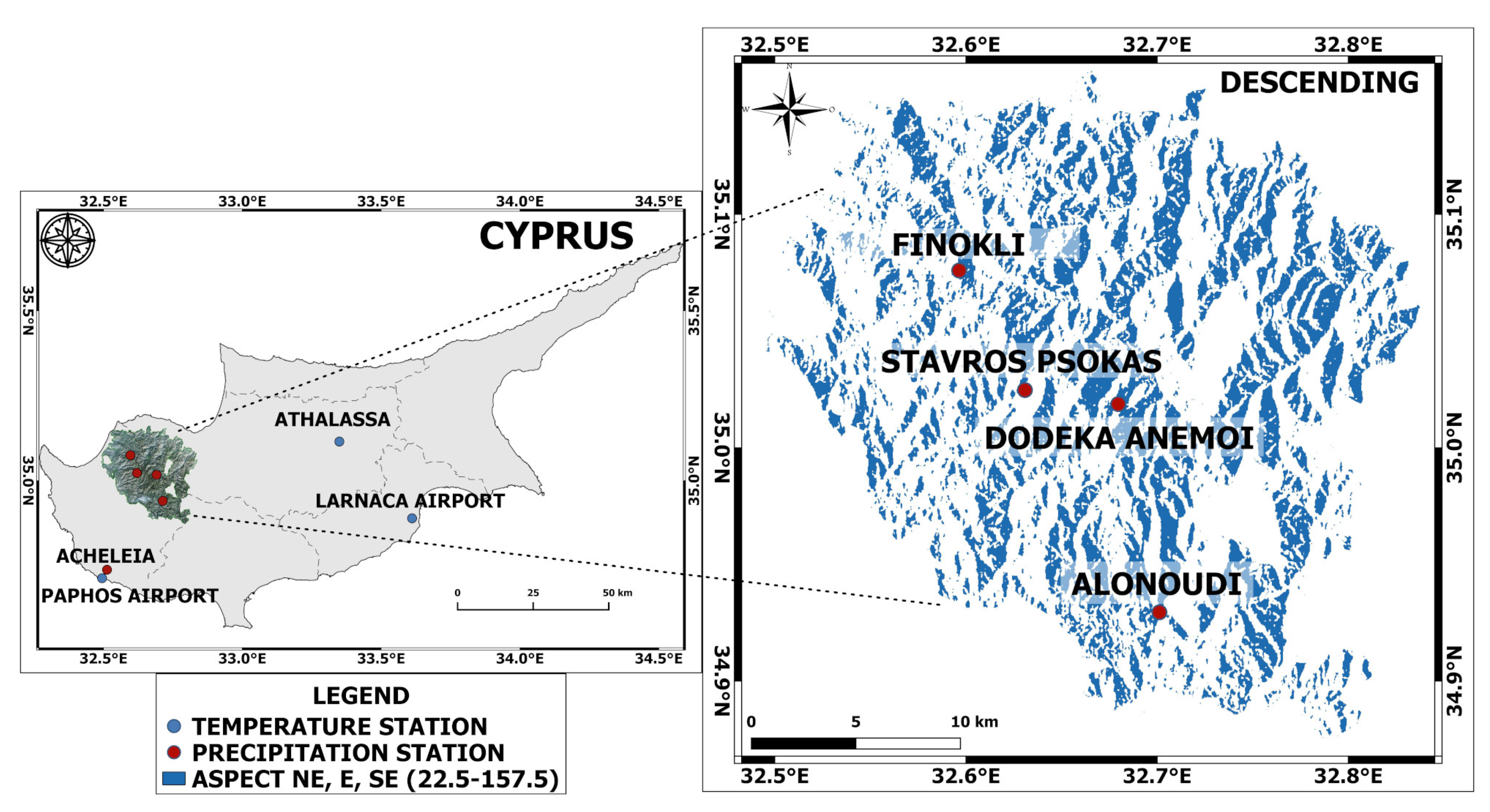According to Shoukri and Zachariadis [5], in comparison to other European regions, the Mediterranean region will be more affected by climate change [5]. Cyprus is the third largest island of the Mediterranean sea [6] and it lies in its north-eastern end (33${}^{\circ }$ east of Greenwich and 35${}^{\circ }$ north of the Equator) [7]. The island has a diversity of microclimates [6] and diverse landscapes [7] that are sufficiently isolated to support a high number of species leading to the formation of endemic biota [7]. According to ancient statements written by historic authors including Eratosthenes (275-195 B.C), Cyprus was rich in forests. The forests in plains were too dense for inhabitation [8,9]. According to a statement provided by A. K. Bovill and D.E Hutchins (1909), the demarcated forests in Cyprus were 10.7% and 19% if scrub-forests were also included [9]. According to Delipetrou et al. [7] (2008), 18.7% of the island is forested. A recent quantitative study showed that 65.62% participants, Cypriot residents, noticed a moderate to very large degradation of Cypriot coniferous forests [10]. The Department of Forests, Cyprus, (2018) also claimed that Cypriot forests are negatively influenced by prolonged droughts occurrences due to climate change. The consequences of the prolonged droughts include high temperatures and a lack of soil moisture leading to intense forest species stress in Cypriot forest ecosystems (Department of Forests, 2018). The impacts of climate change may include alternations in the distribution of forest species, increased forest mortality events, higher fire risk and species extinction [5].

Another potential threat that Cypriot and Mediterranean forests may face due to climate change is the increased attacks from pests. The pine processionary (Thaumetopoea pityocampa) eats the needles of Scots pines (Pinus sylvestris L.) and it is responsible for seasonal defoliation. According to Hódar et al. [11], the attacks of pine processionary (Thaumetopoea pityocampa) to Scots pines (Pinus sylvestris L.) has increased in the Mediterranean region due to climate change. This causes a significant reduction of pine growth as well as some deaths [11]. For example, Toffolo et al. [12] reported significant intense defoliation events and an expansion of the action of the pine processionary in Northern Italy [12]. If there are no extreme weather conditions, the infected pine trees produce new needles and survive [13]. When the pest builds nests on the same tree for 3–4 continuous years, then the tree is negatively influenced, and tree mortality may occur [13]. Pine processionary did not exist in higher elevation areas of the Troodos mountain range, but it is expanding, and its action is strengthened by the persistent drought and warmer weather conditions [13], posing a potential threat to forest species that exist at higher elevations.

According to the “report on the future climate change impact, vulnerability and adaptation assessment for the case of Cyprus”, published in 2016, there are two important climate change threats for Cypriot forests: fires and “dieback of tree species, insect attacks and diseases” [14]. Forest fires are usually the priority of the Department of Forests since they have an immediate effect on the forests. Nevertheless, according to Lemesios et al. [14], both threats have the same vulnerability scores: a very high sensitivity, very high exposure and moderate adaptive capacity. It is, therefore, of crucial importance to study, monitor, model forest health and its resilience, as well as to introduce policies using scientific evidence for preserving forests and a healthy ecosystem. According to Stenlid et al. [15], many anthropogenic factors strengthen forest diseases in Europe, but there is no adequate legislation to limit those factors [15]. For that reason, there is a need to create forecasting models and derive concrete measurements that will add on and improve current knowledge of our forests. These models and the concrete results could be used as scientific evidence for promoting environmentally friendly policies aiming to mitigate the effects of climate change, preserve a healthy ecosystem and consequently maintain social stability and stimulate economic growth.

Phenology is “the study of the timing of recurring biological events, the causes of their timing with regard to biotic and abiotic forces and the interactions among phases of the same or different species”, as defined by the US committee on phenology [16,17]. Phenology observes both plants and animals, as well as seasonal characteristic of natural phenomena [17]. For example, Gittings et al. [18] assessed the phenological indices of phytoplankton blooms in relation to regional ocean warming and showed that warmer conditions were associated with significantly weaker phytoplankton blooms during the winter season [18]. Similar work exists on observing the phenology of various plants and it was shown that climate change conferred shifts to plants’ blooming time [19]. There are also efforts to predict how plants react to warmer conditions and it was shown that plants with higher temperature sensitivity bloomed earlier, but overall, the phenological responses to climate changes were unpredicted [20]. Recently, Wolf et al. [21] showed that a reduction of plant biodiversity caused the shifting of flowering time, thus demonstrating the significance of biotic interactions.

Satellite sensors have been widely used for observing the phenological stages of plants. Gupta et al. [22] showed that apple growth was highly correlated with the Normalized Difference Snow Index (NDSI). Aragones et al. [23] proved that pine species could be classified using phenology-derived classes using the Normalised Difference Vegetation Index (NDVI) in Mediterranean forest. Touhami et al. [24] compared time series NDVI data with precipitation data and showed that land surface phenology was mostly affected by climate parameters during autumn and spring. Frison et al. [25] investigated the potentials of Sentinel-1 synthetic aperture radar (SAR) data for monitoring forest phenology and claimed that phenology could be estimated with a higher accuracy using SAR than optical data.

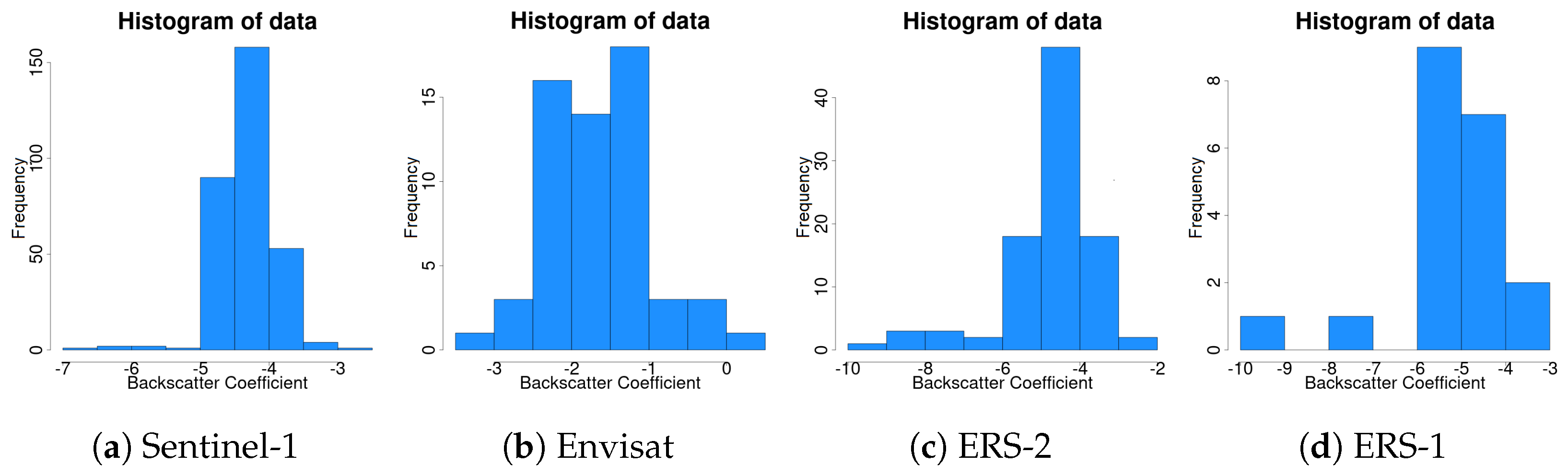
SAR sensors emit microwave energy and record the backscattered signal. Remote sensing is advancing, offering a higher and higher temporal resolution. The Sentinel-1 constellation offers a high temporal resolution of a 6-day repeat cycle making time series analysis of SAR data possible, while previous freely available data included ERS1/2 and Envisat with a repeat cycle of 35 days. Microwave remote sensing is important since microwave radiation can penetrate through objects and can record information, e.g., below a forest canopy, that cannot be acquired by traditional optical remote sensing sensors. The backscattered energy for a particular wavelength is proportional to structure and moisture [26]. While NDVI provides information about the greenness of the plants [26], the values of interferometry coherence can detect vegetation density [27]. Due to the ability of SAR data to derive forest-density-related parameters, the C-band (used in this paper) has been exploited for biomass estimations [28]. 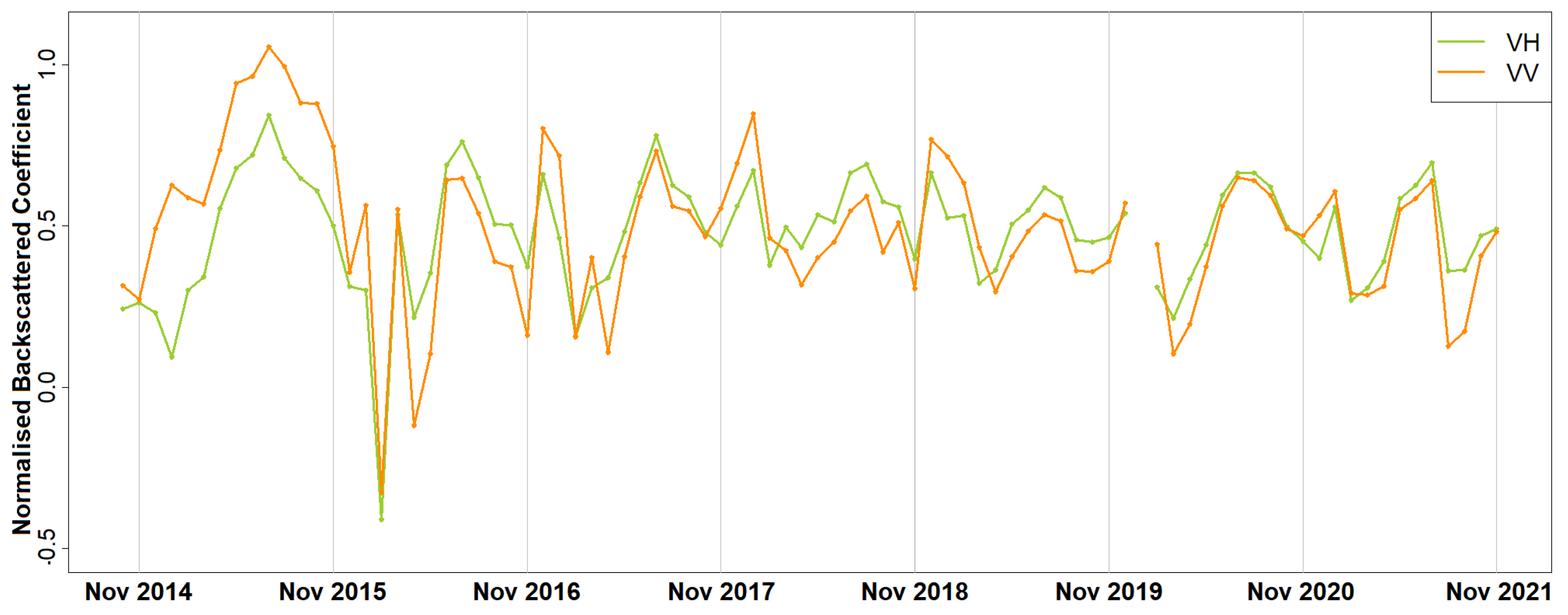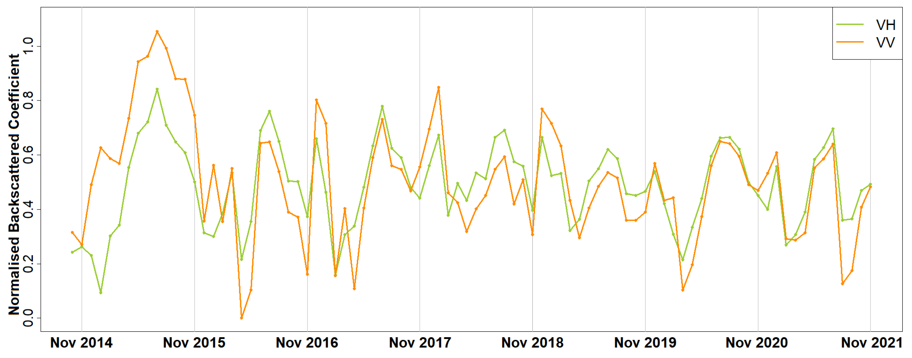Seasonal changes (i.e., phenological changes) observed in evergreen forests using SAR data are hypothesised to be linked to tree foliage and the dielectric constant of the woody component of the trees [29]. If the precipitation is removed or reduced to a minimum, then the tree foliage, water content of the trees and dielectric constant of the wood are the most likely information contained within the backscattering coefficient of the C-band. A time series of C-band SAR data could reveal how these parameters change seasonally and over time. Within a time series of SAR data, the recurrence of phases (i.e., phenology) is measurable as shown in this paper. SAR data were, therefore, selected for observing how the density and water content (e.g., foliage, needles regeneration, fruition) of the forest changes seasonally and over the years [30].

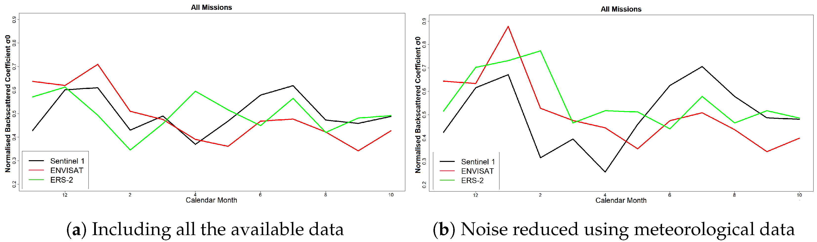
Furthermore, it is important to understand and predict the impacts of climate on forests since the acquired knowledge can be incorporated into decision making [31]. SAR data have been available since 1992 and these data could be used to study climate change effects within a period of 30 years. This study interprets all the available SAR data for the study area but predominantly focuses on the period between November 2014 and October 2021. Within this time period, Sentinel-1 data are available. Sentinel-1 provides a higher temporal resolution [32] while previous missions (ERS1/2, Envisat) present many gaps within the available datasets for the study area. This paper aimed to provide an in-depth understanding of the strengths and limitations of analysing time series SAR data for finding the drivers causing density-, foliage- and/or moisture-related phenological changes in Paphos forest, Cyprus. This was achieved by accomplishing the following objectives:

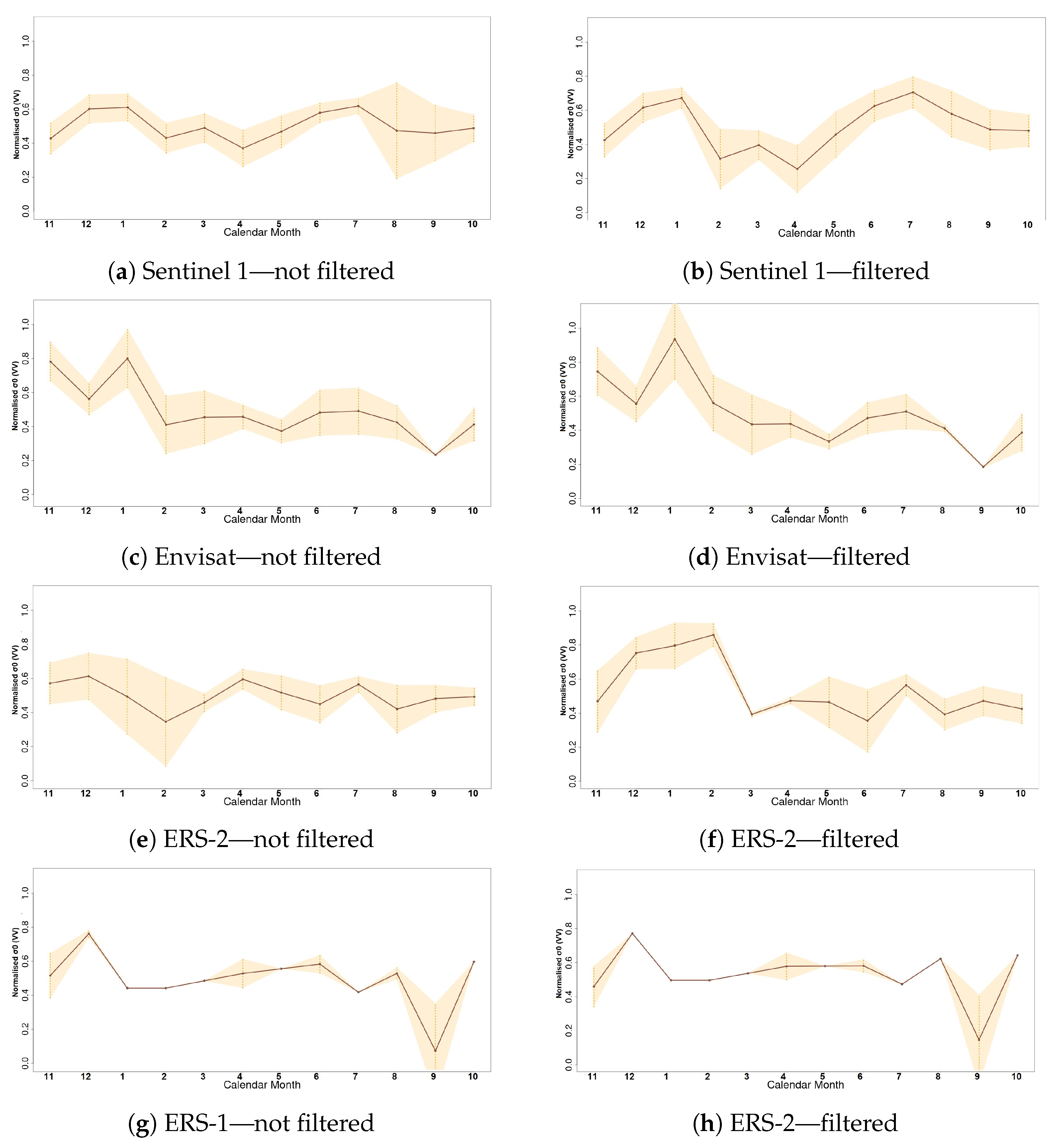
• Study and understand the average annual phenological cycle of Paphos forest and how the time series diagrams could be improved by reducing the effect of precipitation.
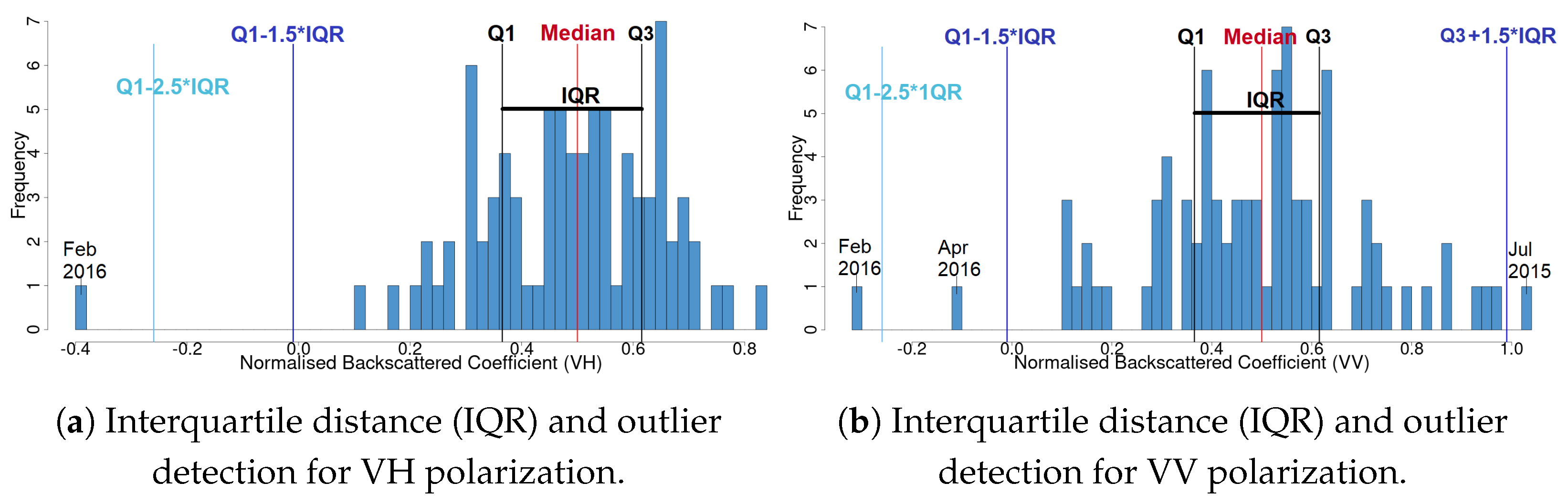
• Detect outliers and justify their importance. Outliers may appear at unusual forest changes that may occur at important events (e.g., a pest attack). They need to be removed before creating predictive models.
• Measure the initiation, duration and termination of detected peaks and link them with the relevant literature to understand the physical parameters that each peak may relate to.
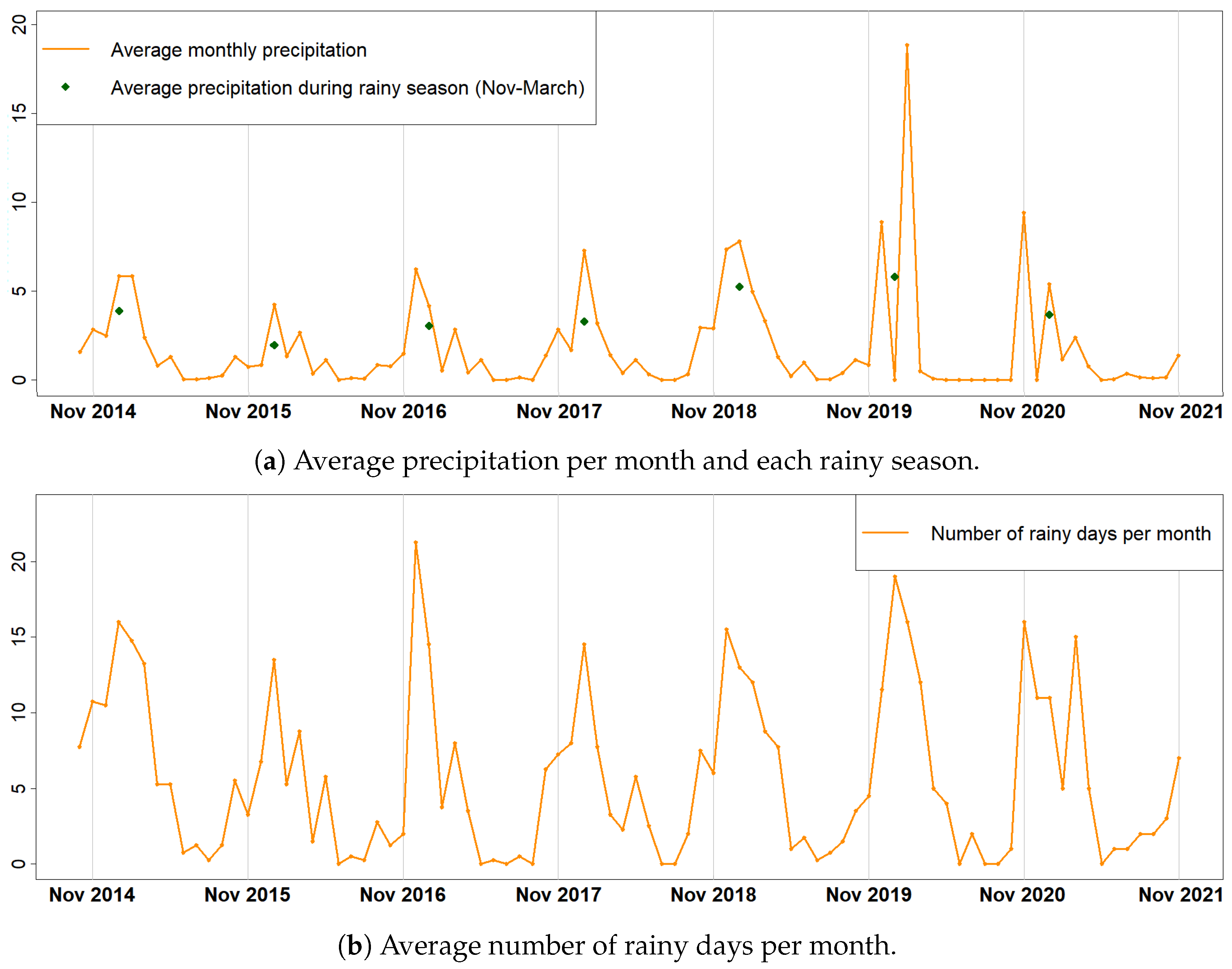
• Investigate the connections between unusual changes in the SAR time series and meteorological thermal and precipitation data.
• Create and evaluate the prediction models and trend lines.
• Investigate the applicability of existing SAR vegetation indexes for time series analysis of data.
• Experiment with filtering approaches and their applicability for removing noise in the SAR data time series diagrams.

2. Material

2.1. SAR Data

Table 1. A summary of the data used in this study showing how many dates were available per mission and how many dates were left after filtering out the dates with high precipitation.

Satellite Mission	Pixel Resolution (m)	Time-Frame	No. of Images	No. of Images per Year	No. of Images after Filtering	No. of Images per Year after Filtering
ERS-1	30	1991–2000	15	1.5	14	1.4
ERS-2	30	1995–2011	79	4.6	66	3.9
Envisat	30	2002–2012	48	4.4	40	3.6
Sentinel1A/B	10	2014–2021	337	50.7	276	39.43

shows a summary of the quantity of acquired data interpreted per satellite mission. As shown, there is a limited availability of data from missions ERS-1/2 and Envisat, but there are adequate data to create a time series from Sentinel-1 data. It is worth noting that the data acquired from Sentinel 1A/B were joint since the instruments are identical but since Sentinel-1B was launched on the 25th of April 2016 [33], less data were available during the first year of investigation. The data were downloaded from the following platforms:

• EO CAT-ESA data services: <https://eocat.esa.int/sec/#data-services-area>
• ASF-Alaska Satellite Facility: <https://asf.alaska.edu/>

As a recall from radar remote sensing, polarization refers to the direction that a microwave signal is oscillating at: vertical (V) or horizontal (H). If the transmitted signal is vertical and the received signal is vertical, the notation VV is used. Similarly, a vertically transmitted signal and horizontally received signal is abbreviated by VH and so forth. ERS-1/2 were single-polarised and only VV was available. Envisat had an alternating polarisation, but for our study area mostly VV data were available and only a few HH images. Sentinel-1 transmits either vertically or horizontally and receives both vertical and horizontal signals. Nevertheless, horizontal-related transmissions (HV and HH) are primarily acquired over wide coastal areas. Therefore, in this study Sentinel-1 data with VV and VH polarisations and ESR1/2 and Envisat data with VV polarisation were used.

2.2. Meteorological Data

In this study, we used daily precipitation data to reduce the effect of moisture in the SAR data and meteorological thermal data to understand whether a change in phenology may relate to the annual act of Thaumetopoea pityocampa and/or drought. According to the Department of Meteorology, Cyprus, a day with precipitation greater than 0.2 is considered a rainy day. Data from four meteorological stations were used for the years 2014 to 2019: three (Finokli-108, Dodeka Anemoi-164, Alonoudi-171) well-distributed within the study area in terms of coverage and elevation changes, and one (Archeleia-81) at the nearby city of Paphos. For 2020 and 2021, data from an additional station (Stavros Psokas-130) were used because the Finokli-108 and Dodeka Anemoi-164 stations had many gaps while acquiring precipitation measurements. The daily precipitation data are not open, but they were provided by the Department of Meteorology, Cyprus upon request. Open data of daily temperatures, that are available from 2010 to 2018, were also used. These open data contain daily temperature measurements from three stations spread around Cyprus (Paphos airport, Larnaka airport and Athalassa) and are available at: <https://www.data.gov.cy/node/1645?language=en>, accessed on 14 October 2021. The locations of the meteorological stations used in this study are given in Figure 1.

2.3. Digital Elevation Model and Aspect Maps

Last but not least, the ASTER Global Digital Elevation Model (GDEM) was used for creating aspect maps, since it has appropriate spatial resolution (30 m). The aspects maps were derived by the digital elevation model and show the steepness and direction of each slope. The aspect maps were required for the definition of the study area (Section 4.1).

3. Study Area

The study area was the state forest “Paphos forest” in Cyprus that lies on the Troodos mountain range and covers around 600 km${}^2$ (Figure 1). According to the maps generated by A. K. Bovilli for the distribution of forests in Cyprus around 1900 [9], the selected study area was forested at that time. Nevertheless, Paphos forest contains old plantations of Calabrian pine (Pinus brutia) dated over 30 years old. These plantations are dense and lack of diversity making the forest more prone to pest attacks. Furthermore, lower elevation areas below (600 m) are defoliated fully annually due to the pine processionary (Thaumetopoea pityocampa). Calabrian pine is the dominant tree species in Paphos forest [7,9]. An important part of this forest ecosystem are smaller trees and shrubs such as Quercus alnifolia, Arbutus andrachne, Olea europaea, Cistus creticus, Ramnus alaternus and Quercus coccifera. There are also some broad-leaved trees, such as the Platanus orientalis, Alnus orientalis, Laurus nobilis, Myrtus communis and bushes, Rubus sanctus [34].

4. Methodology

4.1. Definition of Active Study Area

As aforementioned the study area was Paphos forest, Cyprus. The shapefile defining the boundaries of the forest was provided by the Department of Forest, Cyprus. We chose to work with Paphos forest only since it is the denser and older forest in Cyprus [9], despite the plantations. If we had extended the study area to the entire Troodos mountain range then we would have had noise from villages and constructions. Within Paphos forest, Cyprus, any area that was burnt between 1992 and 2020 was removed, since the forest stands under regeneration are identifiable by remote sensing imagery [35] and could, therefore, produce noise in the time series analysis. Shapefiles about most burnt areas were provided by the Department of Forests, while one fire that occurred on the 6th of March 2003 (north-west of the study area) was mapped and removed utilising the NDVI [36] and normalised burned ratio (NBR) [37] derived from a Landsat image.

Aspects maps were used to select the nonshaded areas in the SAR images. SAR systems emit their signal sidewise and as a result slopes facing away from the radar beam appear as shadows. The shadows are more intense in mountainous areas sometimes making it impossible to analyse the data in the shaded areas. SAR systems observe from the west when the orbit of the satellite is ascending (northward) and from the east when the orbit of the satellite is descending (southward). In the ascending data the nonshaded areas include the north-east, east and south-east slopes ($22.5^{\circ }$–$157.5^{\circ }$) and in the descending data the nonshaded areas include the south-west, west and north-west slopes ($202.5^{\circ }$–$337.5^{\circ }$). For continuity in the observations, the descending SAR data were used in this study. The nonshaded slopes that were aligned with the descending nonshaded data shaped the boundaries of the study area; they are depicted in blue colour in Figure 1. The final active study area is depicted in blue in Figure 1 and its size is 196.36 km${}^2$.

4.2. Preprocessing of SAR Data

4.2.1. SNAP Preprocessing

The data were preprocessed using the ESA SNAP toolbox and a customised python script to ease the massive batch processing. The SNAP graph builder was used for producing three preprocessing pipelines dedicated to each type of satellite image imported (Sentinel-1, Envisat, ERS-1/2). For Sentinel-1, we used “Read -> ThermalNoiseRemoval -> Apply-Orbit-File -> Calibration -> Speckle-Filter -> Terrain-Correction-Write”. For Envisat, we used “ Read -> Apply-OrbitFile-Calibration -> Speckle-Filter -> Terrain-Correction -> Write”. For ERS-1/2, we used “Read -> Apply-Orbit-File -> RemoveAntennaPattern -> Calibration -> Speckle-Filter -> Terrain-Correction -> Write”. The digital numbers (DN) were then converted to decibel (DB) using the formula $DB=10log10\left(abs\right(DN\left)\right)$. The speckle filter selected was a median filter, because forests include high gradient changes and it was, therefore, considered as an appropriate filter since it is good at removing outliers without smoothing the image or enhancing edges. The SNAP graphs were exported, and we wrote a python script that automatically generated a batch file that processed the images in a queue using the gpt command within Command Prompt (<https://github.com/Art-n-MathS/SNAPGraphMassiveProcessing>).

4.2.2. Removing Images with High Precipitation

SAR reflects on both moisture and structure. To reduce the impact of increased moisture produced by precipitation, we filtered out images acquired at increased precipitation. Precipitation data from the meteorological stations (Section 2.2) were used. This was considered necessary since the backscattering coefficient of the radar data is influenced by precipitation/rainfall, as it is implied by studies able to estimate rainfall from analysing radar data [38,39]. Moreover, soil moisture affects a radar signal [40], while in this study, we were predominantly interested in the volume scattering that relates to forest density/foliage. Quegan et al. [41] simulated various conditions and investigated the effect of wet and rough soil in ${\sigma }_{VV}$ in relation to the biomass content of the forest. For forests with a lower biomass, the effect of wet and rough soil was bigger than in forests with a larger biomass (i.e., the reflection was higher when the soil was wet or rough). Considering that the dominant species of Paphos forest is the medium size tree (Pinus brutia) that grows at around 20–35 m, and the shrub/small tree golden oak (Quercus alnifolia) that grows up to 10 m, it is very likely that the coefficients ${\sigma }_{VV}$ and ${\sigma }_{VH}$ will be influenced by wet and rough soil. By performing some tests in the Mediterranean region, where images contain less gradient changes, we were able to understand the effects of precipitation. We concluded that images were influenced during and up to two days after increased precipitation. A combined threshold with weights from those three days was used to classify whether an image should be included into the calculations or removed due to high precipitation. Table 1 shows the numbers of images per missions before and after filtering.

4.2.3. Normalising Backscattering Coefficients

The probability distribution of each satellite was aligned to make the values of the backscattering coefficients comparable between different satellites and lie approximately in the range [0, 1]. Since the backscattering coefficient was normally distributed (see Figure 2), it implied that around 95% of the values lay within four standard deviations from the mean. If we subtract the mean and divide by four standard deviations, then the new signal will have a mean equal to 0 and a standard deviation equal to 1. To increase resilience to outliers (i.e., data that were different from what was expected and unlike the rest of the data), the median and interquartile range (IQR) were used for normalisation instead of the mean and standard deviation [42]. IQR is the difference between the third quartile ($Q3$, 75th percentile) and the first quartile ($Q1$, 25th percentile) [42]. Therefore, the backscattering coefficients were normalised to lie approximately within the range $[0,1]$ as follows:

$$X_n=\frac{X-\mu }{4\times IQR}+0.5$$

(1)

where for each satellite, $X_n$ is the vector of its normalised backscattering coefficients, $\mu$ is its median backscattering coefficients and $IQR$ is the interquartile range.

4.3. Phenological Graphs per Satellite Mission

Assuming that $v(i,j)$ denotes an average backscattering coefficient of month i and year j, the average backscattering coefficient of a satellite mission in month i was calculated as shown in Equation (2), where N is the number of years per satellite mission and each calendar year has a maximum of 12 month—null numbers were removed. The result was a vector with 12 elements ($\mathbf{A}=[A_1,A_2,\dots ,A_{12}]$) representing the average phenological cycle derived from each satellite mission. The average phenological cycles derived for each mission were also comparable—to some extent as explained in the discussion (Section 6.1)—since their probability distributions were aligned.

$$A_i=\frac{{\sum }_{j=1}^{N}v(i,j)}{N}$$

(2)

Due to the increased temporal resolution of Sentinel-1, time series between October 2014 and November 2021 (7 phenological cycles) of both VV and VH polarizations were generated and interpreted deeper than the average phenological graphs.

4.4. Outliers

Outliers are signals that are inconsistent within a dataset. Particular attention should be given to outliers as they may mark important events, e.g., (pest attacks) or could be caused by a system fault/noise. In machine learning, it is important to remove the outliers as they indicate unusual events, and their removal improves predictions. We created the histograms of the backscattering coefficients and used the interquartile (IQR) range to detect the outliers. As the data were normalised, the median was equal to 0.5 and IQR was equal to 0.25 for both ${\sigma }_{VH}$ and ${\sigma }_{VV}$ data. According to Verma and Ranga [42], any data that lie outside the range $[Q1-1.5\times IQR,Q3+1.5\times IQR]$ should be considered as outliers.

To increase the resilience of the predictions/interpretations of Sentinel-1 data, a big outlier appearing at both ${\sigma }_{VH}$ and ${\sigma }_{VV}$ was removed and a new value was estimated using a Kalman filter imputation, since, as shown by Saputra et al. [43], it handles better missing values in comparison to the state-space model ARIMA imputation method. A gap in January 2020 was also filled using the Kalman filter imputation method. The imputation of the new values was applied before the normalisation.

4.5. Measuring Initiation, Duration and Termination of Detected Peaks

To better understand the phenological cycles of Paphos Forest, Cyprus, the initiation, duration and termination of each peak was estimated. We tested two methodologies: (1) the scipy.signal.peak_widths() function available in python and (2) findpeaks() available in R. Both methodologies detect the timing of peaks, as well as the initiation, duration and termination of each peak. Regarding the duration attribute, the first one measures the prominence width of the pulse at a peak. The prominence width is how much a peak stands out in relation to the other peaks. This was not relevant to the duration of each blooming, and it often returned a number greater than 12 months. The second one adds a border so that the end date of one peak timing is the start date of the next one. Because we were looking of annual reoccurring events, the second methodology—findpeaks() of R—was considered appropriate for estimating the duration of each blooming. Attributes were extracted for both (1) the average phenological graphs and (2) the Sentinel-1 time series. The attributes extracted were: the peak timing, the amplitude at the peak, initiation of the peak, termination of the peak, duration and the sum of all the amplitudes between the initiation and the termination of each peak. The tables containing all the results are included in Section 5.1.2.

For each peak extracted, the following related parameters were measured: the peak timings, the normalised backscattering coefficient at the peak, initiation of the peak, termination of the peak and the sum-normalised backscattering coefficient of all the amplitudes between the initiation and termination.

4.6. Investigate Connection between Unusual Changes and Temperature/Precipitation

Weather is an important factor that impacts phenological changes. The Mediterranean climate is warm. Summer is dry. It starts in May and ends in the middle of September. The winter is rainy but mild and starts from the middle of November and lasts till the middle of March. East Mediterranean is influenced by Asia and reaches high temperatures over the summer period, while the summer rainfall does not exceed 5% of the annual rainfall [44]. Using meteorological data, we tried to understand unusual changes in the time series. In personal communication with the Department of Forests, November is considered a critical month in Cyprus for the growth of pine processionary (Thaumetopoea wilkinsonii). To understand the number of peaks per year and whether they related to the pest not surviving cold November, we created the histogram of the average daily temperatures in November and measured their mean and standard deviation. Further, we created a time series of precipitation data and a time series of the number of rainy dates per month in order to understand the effect of drought.

4.7. Prediction and Forecasting

A trend line provides the direction in which the values of a given dataset might move over time. The aim of the prediction was to estimate the amplitude of the annual summer peak usually occurring in July, as well as the annual average backscattering coefficient. The timing of the summer peak was assumed to always be in July as there are limited quantity of data to write prediction models that understand when the summer peak is delayed. The trend estimations were simple linear regression models, i.e., the equation of a straight line that returns the minimum summed, squared Euclidean distance from a given training dataset. In total, seven years of high temporal Sentinel-1 data were available for training and evaluation. We also had two time series (${\sigma }_{VH}$ and ${\sigma }_{VV}$) that were processed separately. Multiple training-testing cases were created. For each test case, the data were divided into training and testing periods. Training data varied from 3 to 6 years, while testing data varied from 1 to 3 years. In some test cases, the first year was discarded, because as shown in Section 5.1.1 the peak of the first phenological year was an outlier in ${\sigma }_{VV}$. Furthermore, it contained one major peak in ${\sigma }_{VH}$ instead of the two that most of the other years had. Despite making some associations with the meteorological thermal data, we did not have enough data to observe what happens in those cases. The results of the various tests were evaluated using the root mean square error (RMSE) and the relevant root mean square error (rRMSE).

4.8. SAR Vegetation Indexes: RVI and RFDI

Vegetation indexes have been widely used for understanding forest health. The Radar Vegetation Index (RVI) (3) [45] and an adjusted Radar Forest Degradation Index (RFDI) (4) were tested. They were calculated using the ${\sigma }_{VV}$ and ${\sigma }_{VH}$ in decibels and then normalised as explained in Section 4.2.

$$RVI=\frac{4{\sigma }_{VH}}{{\sigma }_{VV}+{\sigma }_{VH}}$$

(3)

$$RFDI=\frac{{\sigma }_{VV}-{\sigma }_{VH}}{{\sigma }_{VV}+{\sigma }_{VH}}$$

(4)

4.9. Filtering Experiments

Since SAR data are very sensitive to speckle noise, for the Sentinel-1 high temporal data, we investigated filtering by applying various convolution filters [46]. Let us assume that $x\left[n\right]$ is the average monthly backscattered signal and $h\left[n\right]$ is a discrete convolution kernel with length L. Simultaneously, n goes from one to the size of x. Then, the convoluted (in this case smoothed) SAR signal $y\left[n\right]$ is calculated as shown in Equation (5) [46]. In this paper, the convolution kernels $\{\frac{1}{3}[1,2,1],$$\frac{1}{3}[1,3,1],$$\frac{1}{3}[1,4,1],$$\frac{1}{3}[1,5,1],$$\frac{1}{5}[1,2,3,2,1],$$\frac{1}{5}[1,2,4,2,1],$$\frac{1}{5}[1,2,5,2,1],$$\frac{1}{5}[1,2,6,2,1]\}$ were tested on the SAR Sentinel-1 time series data.

$$y\left[n\right]=\sum _{k=1}^{L}h\left[k\right]x[n-k]$$

(5)

5. Results

5.1. Average Phenological Graphs

The average phenological graphs created for each satellite mission are presented in Figure 3 and Figure 4. It is worth noting that the first calendar month of the phenology of Paphos forest was defined to be November and the last one October. This was decided by observing the average phenological cycles produced from the various missions (peak timings), the life cycle of pine processionary (Thaumetopoea pityocampa), the time series of Calabrian pine and the Mediterranean weather conditions, i.e., the start of the annual rainy season is November. Figure 3 contains two multiline phenological diagrams generated by interpreting ERS-2, Envisat and Sentinel-1 data; the figure on the left-hand side depicts the average phenological cycles before images with high precipitation were discarded and the figure on the right-hand side the average phenological cycles after images with high precipitation were discarded (Section 4.2). Once images with high precipitation were removed, the diagrams appeared to have similar features. Figure 4 shows the average phenological graphs and the standard deviation derived by the VV polarization of ERS-1, ERS-2, Envisat and Sentinel-1 missions before and after filtering out images with high precipitation. Diagrams in both figures were normalised as explained in Section 4.2.3. Two main annual peaks were identified using SAR VV-polarization data from three satellite missions (Figure 3): the first one appears in January and the second one in July. Throughout the paper, we named those two peaks “winter peak” and “summer peak”.

It is further worth noting that even though the data were normalised, a comparison between different ages was relatively feasible. For example, according to Figure 3 the winter peak used to be higher than the summer peak, while nowadays and as shown by the Sentinel-1 data, both peaks have about the same amplitude. Although Sentinel-1 seems to have the highest summer peak in comparison to the older data, it has the smallest winter peak. We cannot assume though that the summer peak has been increased over the years because this could be the result of the applied normalisation (Section 4.2.3). Similarly, we cannot assume there are higher values after filtering, but instead there are relatively greater changes between each month’s backscattering coefficient. Nevertheless, the launched of Sentinel-1 and the revisit cycle of 6 days makes it possible to observe how the two peaks have changed over the last 7 years.

5.1.1. Outliers and Kalman Filter Imputation

Using the IQR outlier detection algorithm (Section 4.4), it was derived that February 2016 was a big outlier in both ${\sigma }_{VH}$ and ${\sigma }_{VV}$ time series, while April 2016 and July 2015 appeared as outliers only in the ${\sigma }_{VV}$ time series (Figure 5).

Figure 6 depicts the time series generated using the normalised backscattering coefficients ${\sigma }_{VH}$ and ${\sigma }_{VV}$ before the Kalman filter imputation was applied, while Figure 7 shows the results of the imputation using the Kalman filter. Two dates were imputed: the big outlier of February 2016 and the gap in January 2020. Comparing the results of the imputation with Figure 6 where the time series includes the outlier of February 2016, the range of the values between November 2016 and November 2019 are stretched after normalisation since the outlier is not affecting them.

Regarding the results in our extended abstract [30], it is worth noting that the mean and standard deviation were used for normalisation and any value less than zero was forced to zero. Additionally, meteorological data were available only until the end of 2019. Therefore, subtle differences may exist.

5.1.2. Measuring Initiation, Duration and Termination of Detected Peaks

We identified peak values for both the average phenological graphs and the Sentinel-1 time series.

Table 2. This table provides the peak timings, the amplitudes at the peak timings, the initiations and terminations of peak timings and their duration in months (widths). The amplitude is the normalised backscattering coefficient (${\sigma }_{VV}$) that approximately lies between the range of [0, 1].

Peak Number	Peak Timing	${\mathit{\sigma }}_{\mathit{VV}}$	Initiation	Termination	Duration	Sum
	Sentinel-1
1	Dec	0.671	Nov	Feb	3	2.027
2	Mar	0.396	Feb	Apr	2	0.967
3	Jul	0.706	Apr	Oct	6	3.591
	Envisat
1	Jan	0.878	Dec	May	5	3.313
2	Jul	0.508	May	Sep	4	2.115
	ERS-2
1	Feb	0.773	Nov	Mar	4	3.187
2	Apr	0.517	Mar	Apr	3	1.934
3	Jul	0.578	Jun	Aug	2	1.483
4	Sep	0.517	Aug	Oct	2	1.468

shows the attributes extracted for each peak from the average phenological graphs derived from the three missions ERS-2, Envisat and Sentinel-1.

Table 3. This table contains information derived from Sentinel-1 data with VH. The period of investigation is Nov 2014 till Oct 2020. For each year, it provides the peak timings, the amplitudes at the peak timings, the initiation and termination of each peak timing, their duration in months, as well as the total/sum amplitude corresponding to each peak (start and end both included). The amplitude is the normalised backscattering coefficient (${\sigma }_{VH}$) that approximately lies in the range [0, 1]—Section 4.2.

Peak Number	Peak Timing	${\mathit{\sigma }}_{\mathit{VH}}$	Initiation	Termination	Duration	Sum
	November 2014–October 2015
1	Jul-15	1.048	Jan-15	Jan-16	12	6.806
	November 2015–October 2016
1	Mar-16	0.552	Jan-16	Apr-16	3	1.078
2	Jul-16	0.919	Apr-16	Nov-16	7	4.062
	November 2016–October 2017
1	Dec-16	0.755	Nov-16	Feb-17	3	1.487
2	Jul-17	0.948	Feb-17	Nov-17	9	4.756
	November 2017–October 2018
1	Jan-18	0.776	Nov-17	Feb-18	3	2.072
2	Mar-18	0.491	Feb-18	Apr-18	2	1.183
3	May-18	0.553	Apr-18	Jun-18	2	1.461
4	Aug-18	0.805	Jun-18	Nov-18	5	3.627
	November 2018–October 2019-testing
1	Dec-18	0.762	Nov-18	Jan-19	2	1.627
2	Feb-19	0.55	Jan-19	Mar-19	2	1.296
3	Jul-19	0.69	Mar-19	Oct-19	7	3.743
	November 2019–October 2020-testing
1	Jan-20	0.579	Oct-19	Mar-20	5	2.226
2	Aug-20	0.763	Mar-20	Dec-20	9	4.786
	November 2020–October 2021-testing
1	Jan-21	0.59	Dec-20	Feb-21	2	1.05
2	Jul-21	0.814	Feb-21	Aug-21	6	3.051

and

Table 4. This table contains information derived from Sentinel-1 data with VV. The period of investigation is Nov 2014 till Oct 2020. For each year, it provides the peak timings, the amplitudes at the peak timings, the initiation and termination of each peak timing, their duration in months, as well as the total/sum amplitude corresponding to each peak (start and end both included). The amplitude is the normalised backscattering coefficient (${\sigma }_{VV}$) that approximately lies in the range [0, 1]—Section 4.2.

Peak Number	Peak Timing	${\mathit{\sigma }}_{\mathit{VV}}$	Initiation	Termination	Duration	Sum
	November 2014–October 2015
1	Jan-15	0.632	Nov-14	Mar-15	4	2.479
2	Jul-15	1.125	Mar-15	Dec-15	9	8.452
	November 2015–October 2016
1	Jan-16	0.558	Dec-15	Feb-16	2	1.197
2	Mar-16	0.543	Feb-16	Apr-16	2	0.862
3	Jul-16	0.656	Apr-16	Nov-16	7	2.657
	November 2016–October 2017
1	Dec-16	0.834	Nov-16	Feb-17	3	1.754
2	Mar-17	0.373	Feb-17	Apr-17	2	0.497
3	Jul-17	0.753	Apr-17	Oct-17	6	3.296
	November 2017–October 2018
1	Jan-18	0.887	Oct-17	Apr-18	6	3.709
2	Aug-18	0.593	Apr-18	Sep-18	5	2.603
3	Oct-18	0.496	Sep-18	Nov-18	2	1.152
	November 2018–October 2019-testing
1	Dec-18	0.796	Nov-18	Apr-19	5	3.088
2	Jul-19	0.526	Apr-19	Oct-19	6	2.771
	November 2019–October 2020-testing
1	Jan-20	0.638	Oct-19	Mar-20	5	2.334
2	Jul-20	0.658	Mar-20	Nov-20	8	3.885
	November 2020–October 2021-testing
1	Jan-21	0.61	Nov-20	Mar-21	4	2.068
2	Jul-21	0.647	Mar-21	Aug-21	5	2.341

show the peak timings, the amplitudes at the peak timings, the initiations and terminations of peak timings and their duration in months (widths) of the Sentinel-1 time series for VH and VV polarisations, respectively.

5.2. Connections between Unusual Changes and Temperature/Precipitation

5.2.1. Selective Statistical Analysis of Meteorological Thermal Data

The most important times of the year that influence phenological changes are autumn and spring. Figure 8 is a histogram of the average daily temperatures acquired at the Paphos airport, Larnaka airport and Athalassa (near Nicosia) meteorological stations at 8 a.m. and 1 p.m. in Novembers. The red horizontal lies depict the mean temperatures recorded each year over November.

Table 5. This table shows the mean, standard deviation and min temperature of November for each available year. The daily temperature was calculated by taking the average measurement at 8:00 a.m. and 1:00 p.m. from three stations: Paphos airport, Larnaka airport and Athalassa.

Year/Temperature	Mean	Standard Deviation	Min
2010	21.9	1.6	18.9
2011	17.2	2.12	14.1
2012	20.7	2.7	17.1
2013	21.1	1.6	17.6
2014	18.8	2.3	13.4
2015	20.8	1.5	16.9
2016	19.5	1.9	16.3
2017	19.4	2.2	15.1
2018	20.4	2.1	16.4

shows statistics about the temperatures recorded in Cyprus in November between 2010 and 2018. The lowest value recorded was 13.4 degrees Celsius on the 25th of November 2014. Even though November 2011 had the lowest average temperature, we did not have Sentinel-1 data for that year. The second lowest temperature was recorded in November 2014. The mean temperature in November from all the available years (2014–2018) was 20.0 degrees Celsius. So, the average temperature of November 2014 was 1.2 degrees Celsius below the average and during that time the lowest average daily temperature was recorded, which was 6.7 degrees Celsius below the overall average. Regarding spring,

Table 6. This table shows the mean and standard deviation of the months March, April, May and June for 2015–2018. The daily temperature was calculated by taking the average measurement at 8:00 a.m. and 1:00 p.m. from three stations: Paphos airport, Larnaka airport and Athalassa.

	March		April		May		June
	Mean	Std	Mean	Std	Mean	Std	Mean	Std
2015	17.00	1.65	19.44	2.97	24.74	2.54	26.85	1.39
2016	18.15	1.84	22.97	2.06	24.11	2.11	29.24	2.75
2017	17.00	19.95	20.62	2.32	24.34	1.81	28.29	1.67
2018	19.24	1.73	23.02	2.21	27.04	2.85	28.56	1.77

shows the mean and standard deviation temperature for the months of March, April, May and June for 2015–2018.

5.2.2. Precipitation and Rainfall Count Days Time Series

Not to be missed is the drought factor. We used the precipitation data requested from the Department of Meteorology (Section 2.2), Cyprus, and created a time series of monthly precipitation data (Figure 9a) and a time series of the number of rainy days per month (Figure 9b). A day with precipitation greater or equal than 0.2 was considered as a rainy day.

5.3. Prediction and Forecasting

Figure 10 and Figure 11 depict the normalised ${\sigma }_{VH}$ and ${\sigma }_{VV}$, respectively, their mean and standard deviation, as well as the estimated trend lines for (1) the summer peaks and (2) the annual means. The trend lines included in the graphs were derived using the period from November 2015 to October 2021 as training datasets. These trend lines were considered appropriate for the visualisation due to the increased quantity of data used for training but were not evaluated.

Table 7. This table provides the results of the various tests conducted for predicting the ${\sigma }_{VH}$ at the summer peak (amplitude of July) using linear regression. The first column indicates the years used for training and a and b are the coefficients derived for the best fit. It also includes the predicted normalised ${\sigma }_{VH}$ for July 2019, July 2020 and July 2021, respectively. NA exists at places where the amplitudes at July 2019 and/or July 2021 was/were used for training the trend lines. RMSE and rRMSE were used to evaluate the prediction.

Training	y = ax + b		July 2019			July 2020			July 2021
Range	a	b	${\mathit{\sigma }}_{\mathit{VH}}$	RMSE	rRMSE	${\mathit{\sigma }}_{\mathit{VH}}$	RMSE	rRMSE (%)	${\mathit{\sigma }}_{\mathit{VH}}$	RMSE	rRMSE (%)
$[1,4]$	−0.0057	1.0914	0.76	0.0701	10.1613	0.6915	0.0703	0.3387	0.6229	0.1911	23.4754
$[2,4]$	−0.0046	1.0498	0.7809	0.091	13.191	0.7253	0.0364	9.2256	0.6697	0.1443	17.7278
$[1,5]$	−0.0069	1.1164	NA	NA	NA	0.6367	0.1251	4.7827	0.5544	0.2595	31.887
$[2,5]$	−0.0068	1.1158	NA	NA	NA	0.637	0.1248	16.4197	0.5549	0.2591	31.8306
$[1,6]$	−0.0054	1.0781	NA	NA	NA	NA	NA	NA	0.6369	0.1771	21.7547
$[2,6]$	−0.0048	1.0455	NA	NA	NA	NA	NA	NA	0.6536	0.1604	19.7002
$[3,6]$	−0.0057	1.0989	NA	NA	NA	NA	NA	NA	0.6316	0.1823	22.3988

and

Table 8. This table provides the results of the various tests conducted for predicting the mean annual ${\sigma }_{VH}$ using linear regression. The first column indicates the years used for training and a and b are the coefficients derived for the best fit. It also includes the predicted average normalised ${\sigma }_{VH}$. NA exists at places where the year “November 2018–October 2019” and/or “November 2019–October2020 was/were used for training. RMSE and rRMSE were used to evaluate the prediction.

Training	y = ax + b		November 2018–October 2019			November 2019–October 2020			November 2020–October 2021
Range	a	b	${\mathit{\sigma }}_{\mathit{VH}}$	RMSE	rRMSE	${\mathit{\sigma }}_{\mathit{VH}}$	RMSE	rRMSE (%)	${\mathit{\sigma }}_{\mathit{VH}}$	RMSE	rRMSE (%)
$[1,4]$	0.0025	0.4312	0.5788	0.071	13.9715	0.6094	0.1323	27.7312	0.6399	0.2091	48.5447
$[2,4]$	0.0035	0.3985	0.6003	0.0924	18.1974	0.642	0.165	34.5772	0.6838	0.253	58.7255
$[1,5]$	0.0015	0.4513	NA	NA	NA	0.5555	0.0785	16.4492	0.5734	0.1426	33.1106
$[2,5]$	0.0014	0.4539	NA	NA	NA	0.5539	0.0768	16.1033	0.571	0.1402	32.5574
$[1,6]$	0.0006	0.4715	NA	NA	NA	NA	NA	NA	0.5214	0.0907	21.0444
$[2,6]$	0.0002	0.4914	NA	NA	NA	NA	NA	NA	0.5094	0.0786	18.2446
$[3,6]$	−0.0007	0.5432	NA	NA	NA	NA	NA	NA	0.4839	0.0532	12.3412

show the results of the predictions for the VH polarisation and

Table 9. This table provides the results of the various tests conducted for predicting the ${\sigma }_{VV}$ during the summer peak (amplitude of July) using linear regression. The first column indicates the years used for training and a and b are the coefficients derived for the best fit. It also includes the predicted normalised ${\sigma }_{VV}$ for July 2019 and July 2020, respectively. NA exists at places where the peak at July 2019 and/or July 2020 was/were used for training. RMSE and rRMSE were used to evaluate the prediction.

Training	y = ax + b		July 2019			July 2020			July 2021
Range	a	b	${\mathit{\sigma }}_{\mathit{VV}}$	RMSE	rRMSE	${\mathit{\sigma }}_{\mathit{VV}}$	RMSE	rRMSE (%)	${\mathit{\sigma }}_{\mathit{VV}}$	RMSE	rRMSE (%)
$[1,4]$	−0.0121	1.1246	0.4206	0.1056	20.0754	0.2749	0.3835	10.4001	0.1292	0.5173	80.0106
$[2,4]$	−0.0027	0.7592	0.604	0.0778	14.7819	0.5719	0.0866	58.2492	0.5398	0.1068	16.5178
$[1,5]$	−0.0104	1.087	NA	NA	NA	0.3575	0.301	13.147	0.2324	0.4141	64.0539
$[2,5]$	−0.0046	0.8156	NA	NA	NA	0.4964	0.1621	45.7083	0.4417	0.2049	31.6919
$[1,6]$	−0.0069	0.9948	NA	NA	NA	NA	NA	NA	0.4309	0.2157	33.36
$[2,6]$	−0.0019	0.7243	NA	NA	NA	NA	NA	NA	0.5699	0.0767	11.8559
$[3,6]$	−0.003	0.7905	NA	NA	NA	NA	NA	NA	0.5427	0.1039	16.0654

and

Table 10. This table provides the results of the various tests conducted for predicting the mean annual ${\sigma }_{VV}$ using linear regression. The first column indicates the years used for training and a and b are the coefficients derived for the best fit. It also includes the predicted average normalised ${\sigma }_{VV}$. NA exists at places where the year ”November 2018–October 2019“ and/or ”November 2019–October2020 was/were used for training. RMSE and rRMSE were used to evaluate the prediction.

Training	y = ax + b		November 2018–October 2019			November 2019–October 2020			November 2020–October 2021
Range	a	b	${\mathit{\sigma }}_{\mathit{VV}}$	RMSE	rRMSE	${\mathit{\sigma }}_{\mathit{VV}}$	RMSE	rRMSE (%)	${\mathit{\sigma }}_{\mathit{VV}}$	RMSE	rRMSE (%)
$[1,4]$	−0.0056	0.6749	0.348	0.1339	27.7796	0.2804	0.1584	36.0977	0.2127	0.1834	46.2978
$[2,4]$	0.0013	0.4314	0.508	0.0262	5.4292	0.5239	0.0851	19.4048	0.5397	0.1436	36.2534
$[1,5]$	−0.0037	0.6379	NA	NA	NA	0.3798	0.059	13.4402	0.3355	0.0606	15.2977
$[2,5]$	0.0008	0.4464	NA	NA	NA	0.5	0.0613	13.9655	0.5092	0.1131	28.5476
$[1,6]$	−0.0031	0.6248	NA	NA	NA	NA	NA	NA	0.3692	0.0269	6.8034
$[2,6]$	−0.0002	0.4769	NA	NA	NA	NA	NA	NA	0.4591	0.063	15.8926
$[3,6]$	−0.0003	0.4801	NA	NA	NA	NA	NA	NA	0.4575	0.0614	15.4884

show the results of the predictions for the VV polarisation. “NA” appears on these tables when the corresponding year was used for training a trend line and, therefore, it was not appropriate to use the same dataset for testing it. The phenological years were labelled from 1 to 7, starting with year “November 2014–October 2015” as number 1. The first year was not included in many tests as it was an outlier and there were not enough data with a similar behaviour to analyse it separately. At each test, we used a different range of years for training and evaluating. For example, if the training range was [2, 4], it implied that the second, third and fourth years were used for training (for deriving the trend lines) and the fifth, sixth and seventh years were used for evaluating the prediction, while the first year was not included in the calculations. It is worth noting that these are preliminary research results since there are many factors to be taken into consideration for reliably predicting those values (including precipitation and temperature) but there is a limited number of years of data.

5.4. Applicability of SAR Vegetation Indexes: RVI and RFDI

The radar vegetation indexes, RVI and RFDI are depicted with black along with ${\sigma }_{VH}$ and ${\sigma }_{VV}$ on Figure 12 and Figure 13, respectively.

5.5. Filtering Experiments

The filtering experiments for the VH-polarization are shown in Figure 14. The kernel $[1,5,1]$ was initially chosen as the best option as it slightly smoothed the signal while causing the least distortion, preserving the most important peaks of the investigation period (Figure 14e). Despite the initial idea that convolutional filtering would smooth the time series and improve the results, it was shown that it may drop important information so we did not use the filtering approach in the preprocessing steps.

6. Discussion

6.1. Average Phenological Graphs

The changes observed in the SAR data were seasonal and we believe that the needles of Calabrian pine played a substantial role in the occurrence of those two peaks. The rainy season starts in November, so it is likely that Calabrian pines absorb water and their dielectric properties change (i.e., increased water content in woody structure) resulting into a higher backscattered SAR signal. Consequently, an increasing trend from around November till January was observed. Pine processionary (Thaumetopoea wilkinsonii) is a pest that eats the needles of the conifers and conifers generate new needles annually. During autumn, the pests are slowly moving their nest upwards so that they can be reached by direct sunlight. This helps them cope with the colder months during the winter [47]. In February, they have already moved their nest on top of the trees and their action is intensified as they are fully grown, and in March they start descending to the ground [47]. That is why there was a big drop in the time series around February, reaching the lowest point in March. According to personal communication with experienced foresters employed by the Department of Forest of Cyprus, Calabrian pine starts to produce new needles annually in April and drops the old ones, with a maximum lifelong around three years old, during the summer. This was aligned with the summer peak. The new needles keep growing until July and, consequently, we observed an upward trend after the decreased backscattering coefficient in the springtime. A decline followed, starting in August, when the Calabrian pine starts dropping the old needles. This was also associated with the annual drought season (Figure 9), which implied that the water content of the trees may also have been reduced. Initially, we thought that cones may also have an impact, but according to [48] the cones ripen between May and June. They may contribute to the increasing trend after the fall around March, but the growth of needles should play a more important role. Not only the summer peak occurred at least one month after the cones were ripe (July) but also warmer spring conditions were associated with a delay of the peak; in contrast warmer spring conditions cause the cones to ripen earlier.

6.2. SAR Time Series with Sentine-1

By comparing the two Sentinel-1 time series, both ${\sigma }_{VH}$ and ${\sigma }_{VV}$ provided useful and different information. Hansen et al. [49] observed large backscatter values in forested areas in both VV and VH. In this study, the mean value of ${\sigma }_{VH}$ was −10.87 decibels and the mean value of ${\sigma }_{VV}$ was −4.32 decibels. Once they were normalised (Equation (1)), they became comparable. By observing Figure 6, we can see that ${\sigma }_{VH}$ had a higher amplitude during the summer peak, while ${\sigma }_{VV}$ had a higher amplitude during the winter peak. Further, Malhi et al. [50] compared ${\sigma }_{VH}$, ${\sigma }_{VV}$ and NDVI for estimating above-ground biomass (AGB) in a tropical Indian forest. Even though standalone VH was proved inefficient in estimating AGB, the data were acquired on the 30th of September 2018. In September at our study area the backscattering coefficients in VV and VH were both low, so we recommend a time series analysis for selecting the best months of the year for forest inventories.

6.3. Outlier

Outliers could be a forest disturbance, so it is important to investigate and understand the drivers of an unusual change. Andronis et al. [34] studied the same area of interest and compared an NDVI time series with land surface temperature (LST). A breakpoint was identified in November 2015 using the bfast algorithm and it was associated with a locust attack. A severe decline of NDVI was observed after this time [34]. The outlier of February 2016 and April 2016 may relate to the same attack; they occurred straight after the breakpoint, and it is likely that the density/foliage-related degradation may have followed the reduction of live vegetation in the forest. Nevertheless, according to the precipitation time series, the year that the outliers appeared was a drought year. The composition of the forest could be destructed during those years and an increased number of pests may appear. Considering also that Paphos forest contains old dense plantations and it consist only of one tree species (once small trees and shrubs are excluded), it is more prone to pest attacks.

6.4. Measuring Initiation, Duration and Termination of Detected Peaks

As defined earlier, a phenological cycle starts in November and ends in October with two main peaks: the summer peak and the winter peak. According to Table 3 and Table 4, those two peaks occurred in December/January and July/August, respectively. There were occasions where smaller peaks existed between the winter and the summer peaks, usually in March, while during the first two phenological years, the winter peaks (January 2015 and January 2016) were missing in the ${\sigma }_{VH}$ time series, but they existed with low amplitudes in the ${\sigma }_{VV}$ time series. It is worth mentioning that those two years contained the outliers detected in Section 4.4, Section 5.1.1 and Section 6.3. July 2015 had a very high amplitude in comparison to the other “summer peaks”. During the year between November 2015 and October 2016 that had the lowest precipitation, the winter peak was missing in ${\sigma }_{VH}$ and there were two outliers in Feb 2016 and April 2016. Therefore, all these observations may relate. A potential relation between the big peak of July 2015 and the pine processionary was discussed in Section 5.2.1. Section 5.2.1 contained the discussion on the selective statistical analysis of meteorological thermal data for understanding the drivers of some changes in the observed phenological changes.

6.5. Connections between Unusual Changes and Temperature/Precipitation

Selective Statistical Analysis of Meteorological Thermal Data

Using meteorological thermal data, we tried to understand why there was one peak in the time series of the ${\sigma }_{VH}$ data during the first phenological year (Nov 2014–Oct 2015), while the following years contained two main peaks (the winter and summer peaks) and occasionally some weaker ones. Figure 8 and Table 5 were generated to understand whether temperatures in November 2014 were lower than the average. As shown in Section 5.2.1, November 2014 was colder in comparison to the other years. Fewer pests survive cold autumn temperatures relevant to the warm Mediterranean climate. Therefore, the effect of the pine processionary eating pine needles, which should have shown in the SAR data with low March backscattering coefficients, was reduced in 2015. This is depicted in the graph from Figure 10. Nevertheless, it is also likely that the phenology may have changed as a result of the drought year in November 2015–March 2016 (Section 5.2.2).

Furthermore, the second main peak, which usually occurs in July, was aligned with the maturity of the new needles and the start of dropping the old ones. It further occurred about one month after fruition time (cone-growing period [30]) of the Calabrian pine that dominates Paphos forest. According to Hawking [51], the blossoming time of Calabrian pine is between March and May. The cones mature between May and June [51]. According to Cleland et al. [19], shifts in the phenology of plants are driven by environmental changes. By analysing the mean and standard deviation of the daily temperatures up to four months before the expected summer peak, it was shown that May 2018 was around 3 degrees Celsius above the average with a high standard deviation, followed by warmer than average March and April (Table 6). This is an indication that the increased temperature during the spring months may have caused the delay of the summer peak in 2018. Thus, we believe that the summer peak relates to the regeneration of the needles rather than the blossoming of the cones since warmer spring conditions make cones mature earlier.

6.6. Precipitation and Rainfall Count Days Time Series

The rainy season is from November to March, and we observed that the drought year of November 2015 was associated with the outlier detected with the IQR detection algorithm. Considering that it includes old plantations that are dense and predominantly consisted of one specie (Pinues Brutia), we suspect that due to the drought, the forest became more prone to pest attacks. Then, in the VH data, we saw a decline in the peaks until a year after the increased rainfall, suggesting that when rainfall increases one year, the benefits of the rain are shown the year after.

6.7. Discussion on Prediction and Forecasting

Overall, for this small dataset, it was not implied that the more SAR data were used for training the trend lines, the more accurate the prediction was. This occurred because the phenology of the forest was influenced by various factors including high temperatures as explained in Section 5.2.1. In parallel, the further away the testing data were from the training data, the lower the accuracy was (e.g., in test case [1,4], the prediction of July 2019 was better than the prediction of July 2020). In most test cases, the rRMSE was less than 20% in predicting the ${\sigma }_{VH}$ and ${\sigma }_{VH}$ of the mean and July for the adjacent year to the training data. Nevertheless, a big evaluation error was observed in predicting ${\sigma }_{VV}$ of July 2020 in test cases [1,4] and [2,5], where the outlier of July 2015 was not used for training and, therefore, a better prediction was expected. The rRMSE values for those two test cases were 45.71% and 58.25%, respectively, while for the test case [1,4], the rRMSE value for predicting July 2019 was 14.78%. As shown in Figure 9, in contrast to the Northern Europe drought, in Cyprus, there was increased precipitation (increased rainfall) between November 2018 and March 2020. We therefore believe that the increased precipitation that preceded conferred increased fruition and/or foliage during the summer period of 2020. This increase in the amplitude of the summer peak influenced the evaluation results. This was also depicted in Figure 10; there was an overall declining trend of the summer peak amplitudes, but the amplitudes of the summer peak in 2020 were bigger than in 2019. Sentinel-1 had high probabilities, while the combination of meteorological data complimented the data and could explain the drivers of phenological alternations. The results indicated here are preliminary, with many limitations due to the length of the time series. Weather conditions should be taken into consideration for reliable predictions. We believe that in the following years, with the availability of longer time series, more specialised models will emerge.

6.8. Applicability of SAR Vegetation Indexes: RVI and RFDI

By observing Figure 12 and Figure 13 and the equations of RVI and RFDI, those indices were considered not applicable for the observation of time series phenological changes. RVI created some inconsistencies in the high values that did not necessarily imply a high structure. For example, if the ${\sigma }_{VH}$ was low and there was a big difference between ${\sigma }_{VV}$ and ${\sigma }_{VH}$, then RVI took a high value (see December 2014). Vice versa, if ${\sigma }_{VH}$ was high but there was a difference between the two, then RVI took a much lower value than both ${\sigma }_{VH}$ and ${\sigma }_{VV}$. Additionally, $RFDI$ occasionally exaggerated the differences between ${\sigma }_{VH}$ and ${\sigma }_{VV}$. For instance, July 2015 had a high reflectance at both ${\sigma }_{VH}$ and ${\sigma }_{VV}$ and $RFDI$ returned a low value, not representing the high structural/moisture backscattering information acquired by the sensor. Similarly, May and July had low values (small denominator) resulting in high RFDI values; nevertheless, low ${\sigma }_{VH}$ and ${\sigma }_{VV}$ implied a low structure and moisture. Additionally, the phenological repetitions depicted in ${\sigma }_{VH}$ and ${\sigma }_{VV}$ seemed to vague when $RVI$ and $RFDI$ were calculated. For those reasons, we were hesitant about the reliability of those indexes in observing phenology.

6.9. Filtering

To avoid dropping important details, the filtering step was not included in the final processing pipeline. The selected filtering kernel was dropping one of the two peaks in ${\sigma }_{VH}$ between January 2018 and August 2018. The summer peak usually occurs in July but there was a delay in summer 2018. During that delay, there were two small peaks between the winter and the summer peak—something unusual. So, we suspect that those two small peaks may be associated with the high spring temperatures of the same year (Section 5.2.1) and the delay of the summer spring. When there are high temperature during or straight after winter, plants can be confused and start blossoming earlier than expected. When a cold day follows an unusually hot day, that can be destructive for the plant. Therefore, it is very important to observe small unusual peaks since their appearance may indicate that the forest is suffering or altering. Even though we did not include this filtering steps in the processing chain, it is important to mention it to help future researchers understand the process.

7. Conclusions

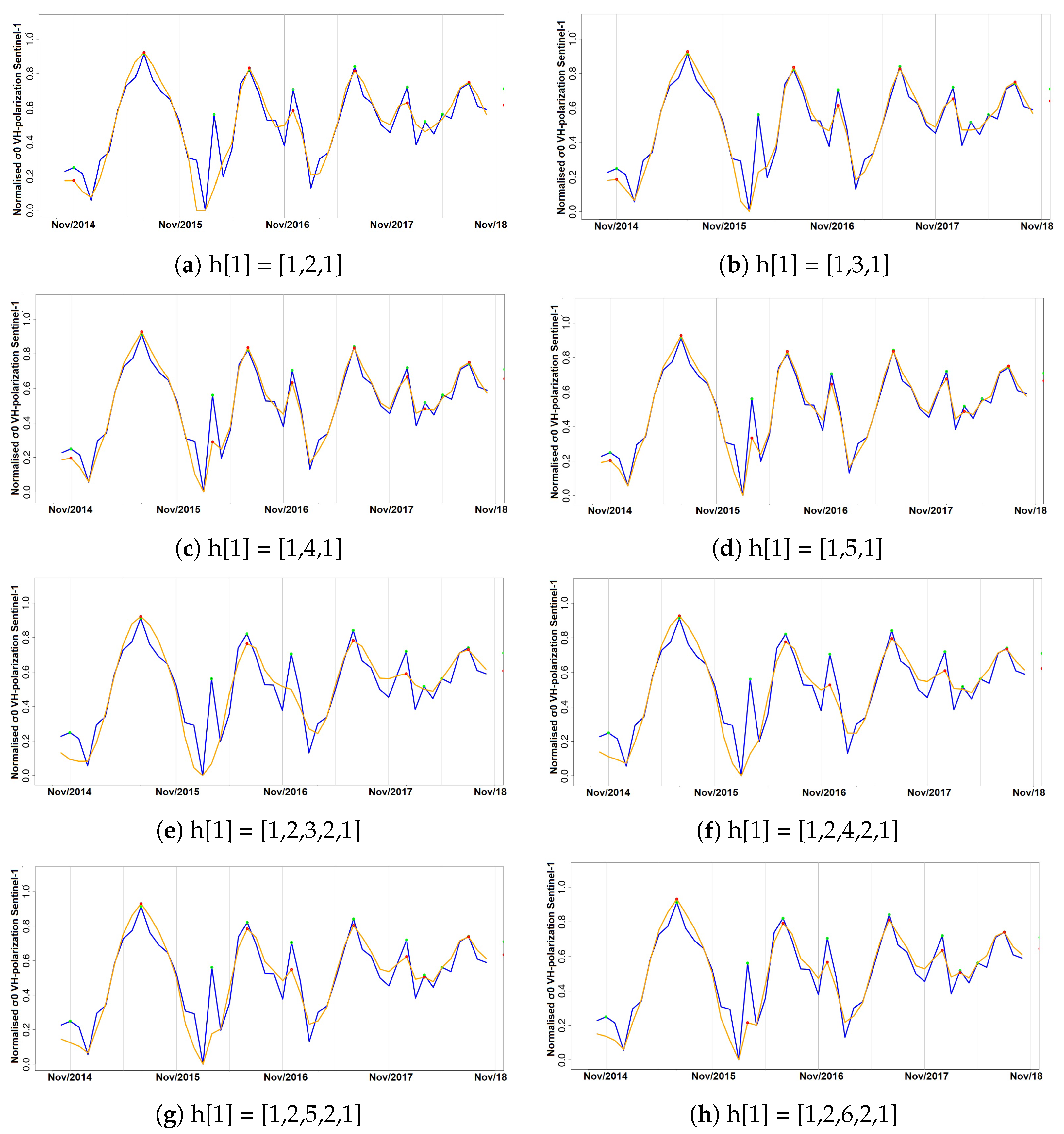
The results of this paper both agree with and adds to the existing literature. As in [25], who claimed that phenology can be estimated with higher accuracy using SAR than optical data. It was shown that phenological diagrams derived with spaceborne SAR data of Paphos forest, Mediterranean sea, Cyprus, contained two major peaks instead of one identified with optical imagery [34]. After a direct communication with experienced foresters from the Department of Forests, Cyprus, it was concluded that the most reasonable explanation for the summer peak was the annual regeneration of the needles and the drop of the old ones. Furthermore, similarly to [24], we showed that autumn and spring climatic conditions play a substantial role in changes presented in land surface phenology. Thus, if the temperature in May is high, then there may be a delay of the summer peak. 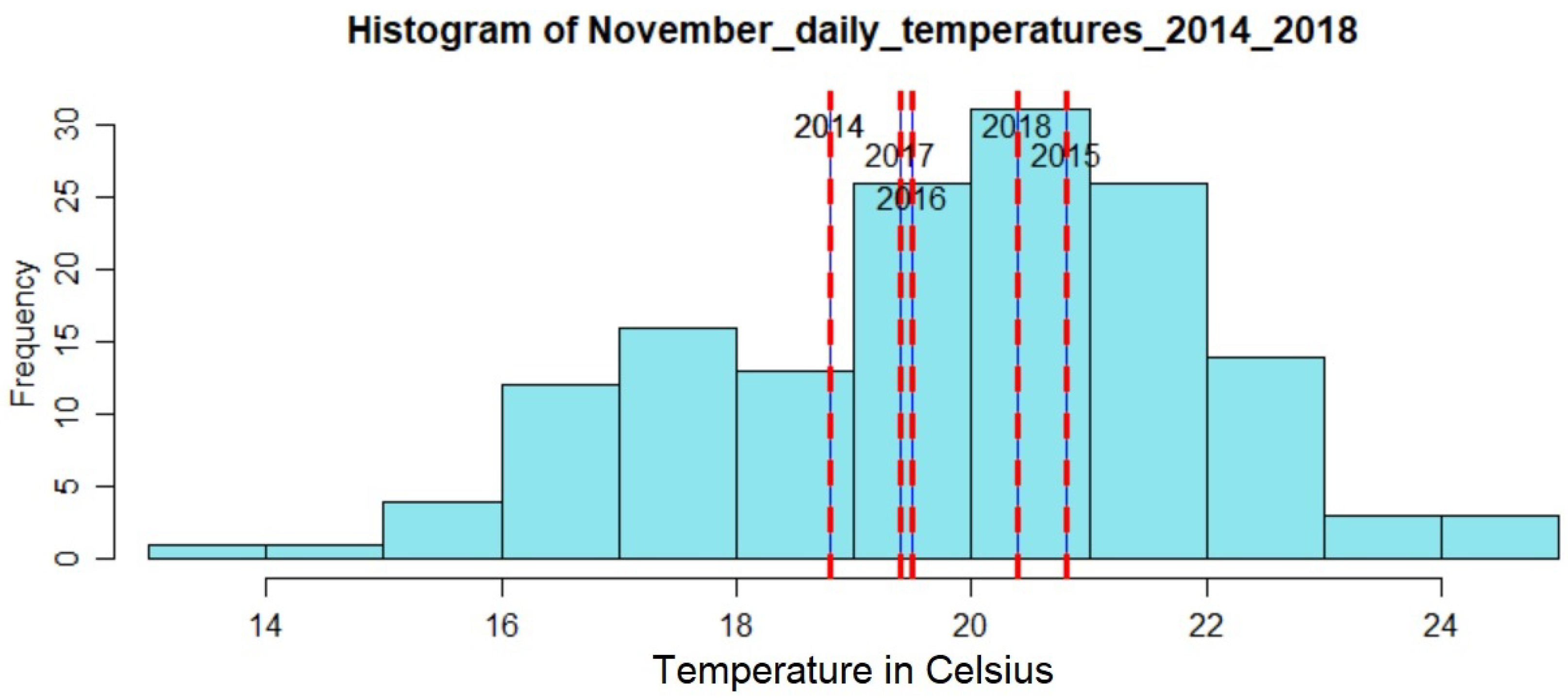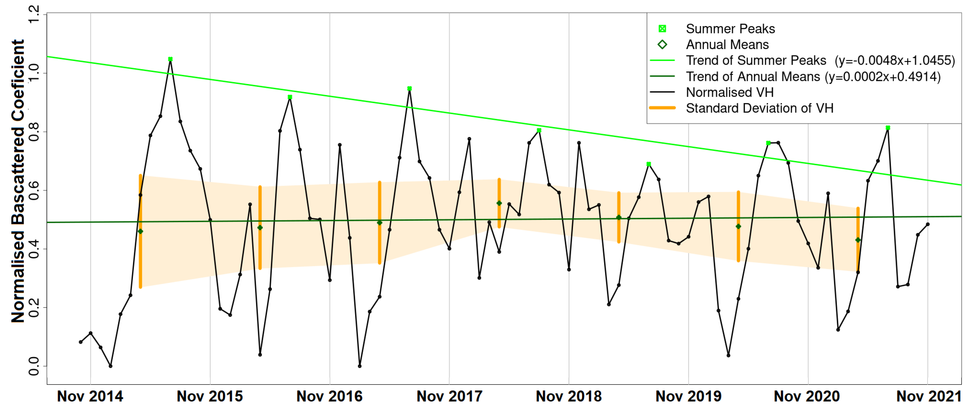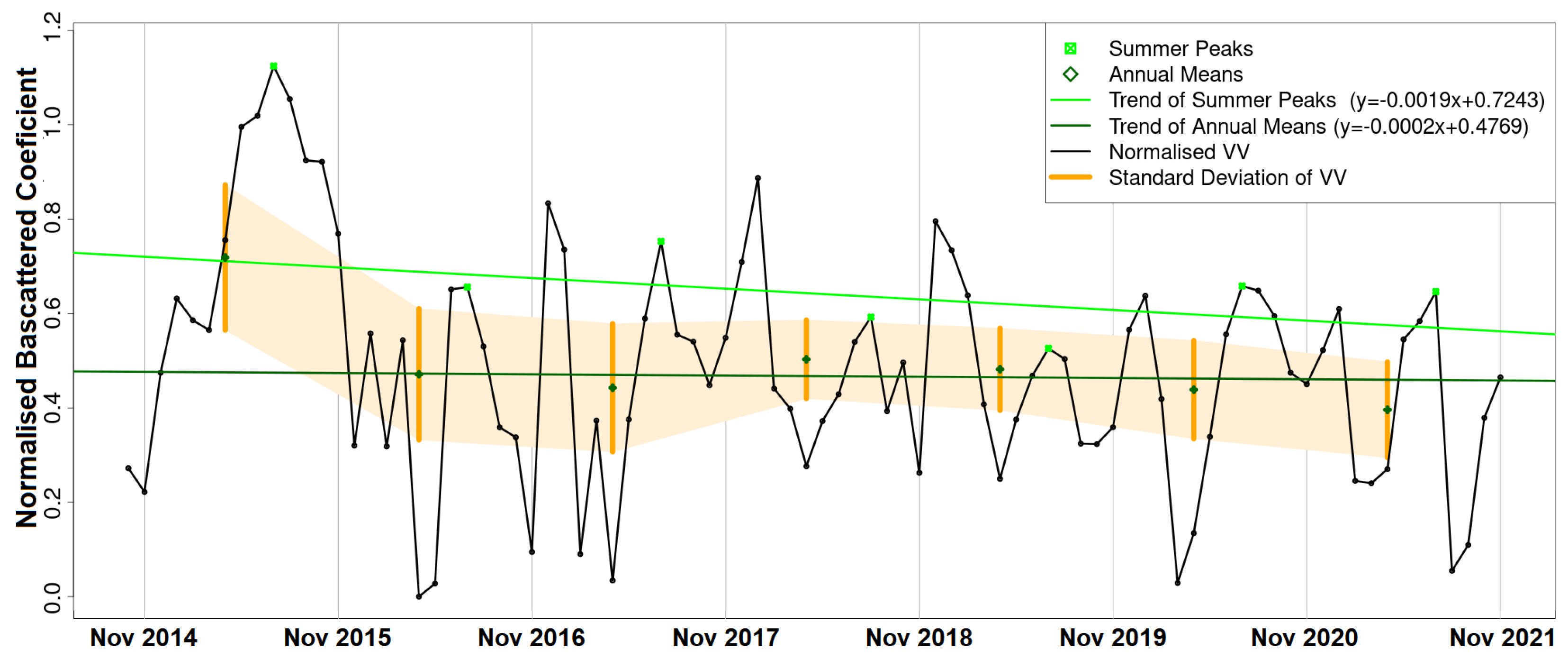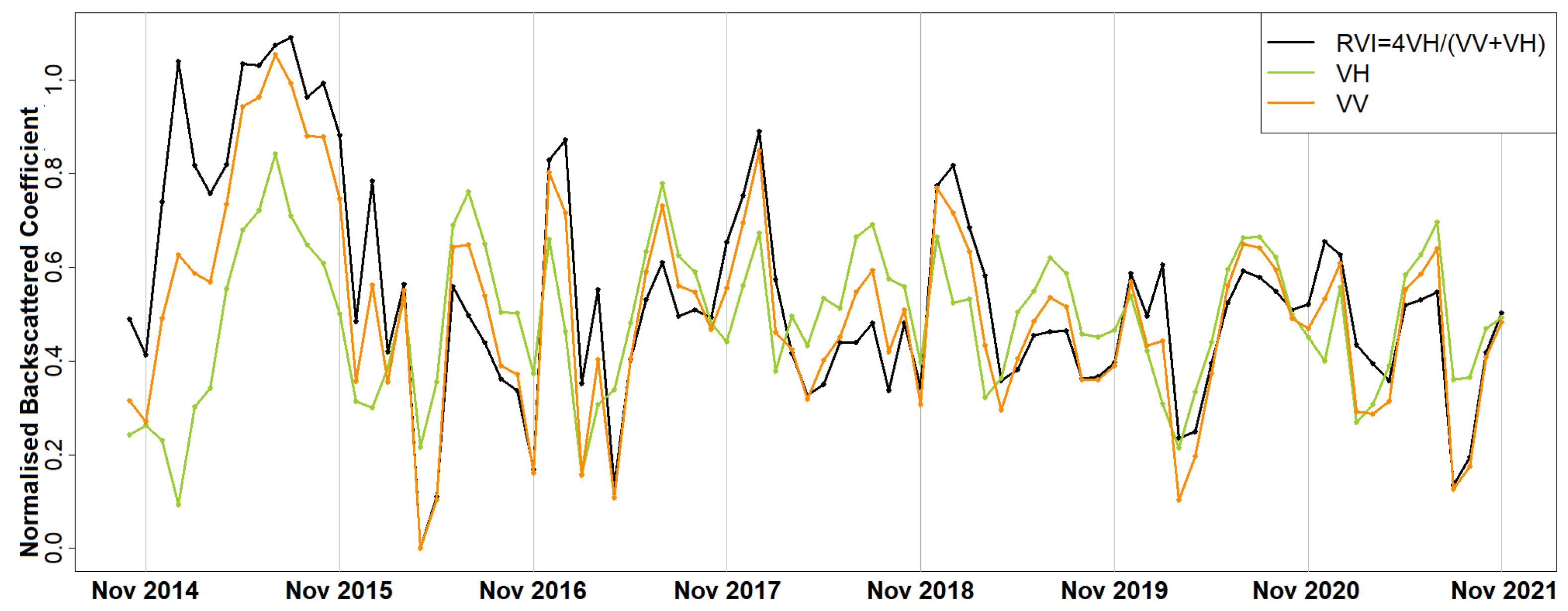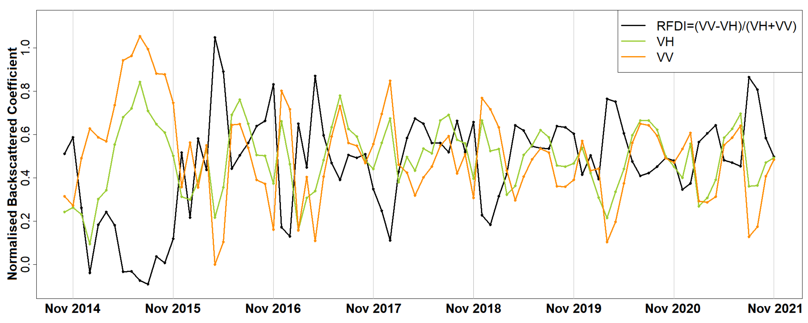Additionally, low temperatures in November may relate to a decreased action of the pine processionary (Thaumetopoea pityocampa) around February and consequently the appearance of one major peak, instead of two, over a phenological year (November-October). Equally important was the association of the rainy season of November 2015–March 2016 that drought (reduced average precipitation) existed with the outliers of February 2016 and April 2016. Secondary conclusions of this work include: a preprocessing that includes smoothing of signals can influence the quality of the results by dropping small peaks that may be important; the radar vegetation indexes (RVI and RFDI) were considered unreliable for time series phenological observations of forests, and in contrast to RVI and RFDI, both ${\sigma }_{VH}$ and ${\sigma }_{VV}$ returned high amplitudes and became comparable once normalised; finally, the detection of peak amplitude and mean backscattering coefficient was possible using trend lines but the time series was short and the trend was highly sensitive to other factors (e.g., precipitation) producing high rRMSE values. Overall, the launch of Sentinel-1 brought new research opportunities for observing the phenological changes of forests. After some more years of Sentinel-1 operation, when the period of investigation is longer and more data are available for the time series analysis, the use of advanced machine/deep learning techniques [52] and signal processing approaches could improve prediction. Combining multisensor/multimodal data improves prediction [50,53]. Therefore, combining satellite multisensor, ground-truth and other spaceborne data in the time series analysis are soon expected to emerge for a better understanding and modelling of the drivers of phenological changes. This will further support climate-related research.

References

1. Gray, J.; Dautel, H.; Estrada-Peña, A.; Kahl, O.; Lindgren, E. Effects of climate change on ticks and tick-borne diseases in Europe. Interdiscip. Perspect. Infect. Dis. 2009, 2009, 593232. [Google Scholar] [CrossRef] [PubMed]
2. Ju, R.T.; Gao, L.; Wei, S.J.; Li, B. Spring warming increases the abundance of an invasive specialist insect: Links to phenology and life history. Sci. Rep. 2017, 7, 1–12. [Google Scholar] [CrossRef] [PubMed] [Green Version]
3. Flannigan, M.D.; Stocks, B.J.; Wotton, B.M. Climate change and forest fires. Sci. Total Environ. 2000, 262, 221–229. [Google Scholar] [CrossRef]
4. Read, D.J.; Freer-Smith, P.; Morison, J.; Hanley, N.; West, C.; Snowdon, P. Combating Climate Change: A Role for UK Forests. An Assessment of the Potential of the UK’s Trees and Woodlands to Mitigate and Adapt to Climate Change; The Stationery Office Limited: Edinburgh, UK, 2009. [Google Scholar]
5. Shoukri, E.; Zachariadis, T. Climate change in Cyprus: Impacts and adaptation policies. Cyprus Econ. Policy Rev. 2012, 6, 21–37. [Google Scholar]
6. Thirgood, J.V. Cyprus: A Chronicle of Its Forests, Land and People; University of British Columbia Press: Vancouver, BC, USA, 1987. [Google Scholar]
7. Delipetrou, P.; Makhzoumi, J.; Dimopoulos, P.; Georghiou, K. Mediterranean Island Landscapes: Natural and Cultural Approaches: Cyprus. Springer Science + Business Media B.V.: Berlin/Heidelberg, Germany, 2008; pp. 170–203. [Google Scholar]
8. Meikle, R.D. Flora of Cyprus. Volume One. In Flora of Cyprus. Volume One; Bentham-Moxon Trust, Royal Botanic Gardens: Kew, UK, 1977. [Google Scholar]
9. Holmboe, J. Studies on the Vegetation of Cyprus: Based upon Researches during the Spring and Summer 1905. Bergens Museums, John Griegs: Bergens, Norway, 1914; Volume 10. [Google Scholar]
10. Miltiadou, M.; Antoniou, E.; Theocharidis, C.; Danezis, C. Do People Understand and Observe the Effects of Climate Crisis on Forests? The Case Study of Cyprus. Forests 2021, 12, 1152. [Google Scholar] [CrossRef]
11. Hódar, J.A.; Castro, J.; Zamora, R. Pine processionary caterpillar Thaumetopoea pityocampa as a new threat for relict Mediterranean Scots pine forests under climatic warming. Biol. Conserv. 2003, 110, 123–129. [Google Scholar] [CrossRef]
12. Toffolo, E.P.; Bernardinelli, I.; Stergulc, F.; Battisti, A. Climate change and expansion of the pine processionary moth, Thaumetopoea pityocampa, in northern Italy. IUFRO Work. Party 2006, 7, 331–340. [Google Scholar]
13. Adeilini. Pityocampa, the Reason Pine Trees Get Dry. Kathimerini. Available online: https://www.kathimerini.com.cy/gr/periballon/pityokampi-i-apeili-ton-peykon (accessed on 2 February 2021).
14. Lemesios, G.; Giannakopoulos, C.; Petrakis, M. CYPADAPT: Development of a National Strategy for Adaptation to Climate Change Adverse Impacts in Cyprus. 2014. Available online: http://uest.ntua.gr/cypadapt/wp-content/uploads/DELIVERABLE3.4.pdf (accessed on 20 August 2018).
15. Stenlid, J.; Oliva, J.; Boberg, J.B.; Hopkins, A.J. Emerging diseases in European forest ecosystems and responses in society. Forests 2011, 2, 486–504. [Google Scholar] [CrossRef]
16. Lieth, H. Phenology and Seasonality Modeling; Springer Science & Business Media: New York, NY, USA, 2013; Volume 8. [Google Scholar]
17. Hudson, I.L.; Keatley, M.R. Phenological Research. Methods for Environmental and Climate Change Analysis; Springer: Berlin/Heidelberg, Germany, 2010. [Google Scholar]
18. Gittings, J.A.; Raitsos, D.E.; Krokos, G.; Hoteit, I. Impacts of warming on phytoplankton abundance and phenology in a typical tropical marine ecosystem. Sci. Rep. 2018, 8, 1–12. [Google Scholar] [CrossRef]
19. Cleland, E.E.; Chuine, I.; Menzel, A.; Mooney, H.A.; Schwartz, M.D. Shifting plant phenology in response to global change. Trends Ecol. Evol. 2007, 22, 357–365. [Google Scholar] [CrossRef] [PubMed]
20. Wolkovich, E.M.; Cook, B.I.; Allen, J.M.; Crimmins, T.M.; Betancourt, J.L.; Travers, S.E.; Pau, S.; Regetz, J.; Davies, T.J.; Kraft, N.J. Warming experiments underpredict plant phenological responses to climate change. Nature 2012, 485, 494–497. [Google Scholar] [CrossRef] [PubMed]
21. Wolf, A.A.; Zavaleta, E.S.; Selmants, P.C. Flowering phenology shifts in response to biodiversity loss. Proc. Natl. Acad. Sci. USA 2017, 114, 3463–3468. [Google Scholar] [CrossRef] [PubMed] [Green Version]
22. Gupta, H.; Kaur, L.; Asra, M.; Avtar, R.; Reddy, C.S. MODIS NDVI Multi-Temporal Analysis Confirms Farmer Perceptions on Seasonality Variations Affecting Apple Orchards in Kinnaur, Himachal Pradesh. Agriculture 2021, 11, 724. [Google Scholar] [CrossRef]
23. Aragones, D.; Rodriguez-Galiano, V.F.; Caparros-Santiago, J.A.; Navarro-Cerrillo, R.M. Could land surface phenology be used to discriminate Mediterranean pine species? Int. J. Appl. Earth Obs. Geoinf. 2019, 78, 281–294. [Google Scholar] [CrossRef]
24. Touhami, I.; Moutahir, H.; Assoul, D.; Bergaoui, K.; Aouinti, H.; Bellot, J.; Andreu, J.M. Multi-year monitoring land surface phenology in relation to climatic variables using MODIS-NDVI time-series in Mediterranean forest, Northeast Tunisia. Acta Oecologica 2022, 114, 103804. [Google Scholar] [CrossRef]
25. Frison, P.L.; Fruneau, B.; Kmiha, S.; Soudani, K.; Dufrene, E.; Le Toan, T.; Koleck, T.; Villard, L.; Mougin, E.; Rudant, J.P. Potential of Sentinel-1 data for monitoring temperate mixed forest phenology. Remote Sens. 2018, 10, 2049. [Google Scholar] [CrossRef] [Green Version]
26. Woodhouse, I.H. Introduction to Microwave Remote Sensing. CRC Press, Taylor & Francis Group: Boca Raton, FL, USA, 2017. [Google Scholar]
27. Bai, Z.; Fang, S.; Gao, J.; Zhang, Y.; Jin, G.; Wang, S.; Zhu, Y.; Xu, J. Could vegetation index be derive from synthetic aperture radar?–the linear relationship between interferometric coherence and NDVI. Sci. Rep. 2020, 10, 1–9. [Google Scholar] [CrossRef] [PubMed] [Green Version]
28. Sarker, M.L.R.; Nichol, J.; Iz, H.B.; Ahmad, B.B.; Rahman, A.A. Forest biomass estimation using texture measurements of high-resolution dual-polarization C-band SAR data. IEEE Trans. Geosci. Remote Sens. 2012, 51, 3371–3384. [Google Scholar] [CrossRef]
29. Ahern, F.J.; Leckie, D.J.; Drieman, J.A. Seasonal changes in relative C-band backscatter of northern forest cover types. IEEE Trans. Geosci. Remote Sens. 1993, 31, 668–680. [Google Scholar] [CrossRef]
30. Miltiadou, M.; Theocharidis, C.; Karathanassi, V.; Agapiou, A.; Nikolaidis, M.; Danezis, C. Understanding phenological changes of coniferous forests in Cyprus using time-series of SAR data from 2015 till 2020. In Proceedings of the Silvilaser Conference, Vienna, Austria, 28–30 September 2021. [Google Scholar] [CrossRef]
31. Keenan, R.J. Climate change impacts and adaptation in forest management: A review. Ann. For. Sci. 2015, 72, 145–167. [Google Scholar] [CrossRef] [Green Version]
32. Geudtner, D.; Torres, R.; Snoeij, P.; Davidson, M.; Rommen, B. Sentinel-1 system capabilities and applications. In Proceedings of the 2014 IEEE Geoscience and Remote Sensing Symposium, Quebec City, QC, Canada, 13–18 July 2014; pp. 1457–1460. [Google Scholar] [CrossRef]
33. Potin, P.; Rosich, B.; Grimont, P.; Miranda, N.; Shurmer, I.; O’Connell, A.; Torres, R.; Krassenburg, M. Sentinel-1 mission status. In Proceedings of the EUSAR 2016: 11th European Conference on Synthetic Aperture Radar, Hamburg, Germany, 6–9 June 2016; pp. 1–6. [Google Scholar]
34. Andronis, V.; Karathanassi, V.; Tsalapati, V.; Kolokoussis, P.; Miltiadou, M.; Danezis, C. Time series analysis of Landsat data for investigating the relationship between land surface temperature and forest changes. The case study of Paphos forest. Remote Sens. 2022, 14, 1010. [Google Scholar] [CrossRef]
35. Akbari, B.; Solberg, S.; Puliti, S. Mutitemporal Sentinel-1 and Sentinel-2 Images for Characterization and Discrimination of Young Forest Stands Under Regeneration in Norway. IEEE J. Sel. Top. Appl. Earth Obs. Remote Sens. 2021, 14, 5049–5063. [Google Scholar] [CrossRef]
36. Rouse, J.W.; Haas, R.H.; Schell, J.A.; Deering, D.W.; Harlan, J.C. Monitoring the Vernal Advancement and Retrogradation (Green Wave Effect) of Natural Vegetation; NASA/GSFC Type III Final Report, Greenbelt, Md; Texas A & M University: College Station, TX, USA, 1974; Volume 371. [Google Scholar]
37. Chuvieco, E.; Martin, M.P.; Palacios, A. Assessment of different spectral indices in the red-near-infrared spectral domain for burned land discrimination. Int. J. Remote Sens. 2002, 23, 5103–5110. [Google Scholar] [CrossRef]
38. Lin, I.I.; Alpers, W.; Khoo, V.; Lim, H.; Lim, T.K.; Kasilingam, D. An ERS-1 synthetic aperture radar image of a tropical squall line compared with weather radar data. IEEE Trans. Geosci. Remote Sens. 2001, 39, 937–945. [Google Scholar] [CrossRef]
39. Steiner, M.; Smith, J.A.; Burges, S.J.; Alonso, C.V.; Darden, R.W. Effect of bias adjustment and rain gauge data quality control on radar rainfall estimation. Water Resour. Res. 1999, 35, 2487–2503. [Google Scholar] [CrossRef]
40. Baghdadi, N.; Aubert, M.; Cerdan, O.; Franchistéguy, L.; Viel, C.; Eric, M.; Zribi, M.; Desprats, J.F. Operational mapping of soil moisture using synthetic aperture radar data: Application to the Touch basin (France). Sensors 2007, 7, 2458–2483. [Google Scholar] [CrossRef] [PubMed]
41. Quegan, S.; Le Toan, T.; Yu, J.J.; Ribbes, F.; Floury, N. Multitemporal ERS SAR analysis applied to forest mapping. IEEE Trans. Geosci. Remote Sens. 2000, 38, 741–753. [Google Scholar] [CrossRef]
42. Verma, A.; Ranga, V. CoSec-RPL: Detection of copycat attacks in RPL based 6LoWPANs using outlier analysis. Telecommun. Syst. 2020, 75, 43–61. [Google Scholar] [CrossRef]
43. Saputra, M.; Hadi, A.; Riski, A.; Anggraeni, D. Handling Missing Values and Unusual Observations in Statistical Downscaling Using Kalman Filter; Journal of Physics: Conference Series; IOP Publishing: Bristol, UK, 2021; Volume 1863, p. 012035. [Google Scholar]
44. Nicolaou, C. Wild Mammals of Cyprus; Cyprus Forestry Association: Nicosia, Cyprus, 2007; pp. 9–15. [Google Scholar]
45. Le Minh, H.; Van, T.V.; Asnh, T.T. Using dual-polarization Sentinel-1A for mapping vegetation types in Daklak, Vietnam. In Proceedings of the 40th Asian Conference on Remote Sensing (ACRS 2019), Daejeon, Korea, 14–18 October 2019. [Google Scholar]
46. Burrus, C.S.; Parks, T. Convolution Algorithms; Citeseer: New York, NY, USA, 1985. [Google Scholar]
47. Kapantais, M. Spring arrived and pityocampa arrived from the pines. dasarxeio 2020. Available online: https://dasarxeio.com/2020/02/23/75768/ (accessed on 20 December 2020).
48. Tsintides, T.C.; Hadjikyriakou, G.N.; Christodoulou, C.S. Trees and Shrubs in Cyprus; Foundations Anastasios G. Leventis-Cyprus Forest Association: Lefkosia, Cyprus, 2002. [Google Scholar]
49. Hansen, J.N.; Mitchard, E.T.; King, S. Assessing forest/non-forest separability using Sentinel-1 c-band synthetic aperture radar. Remote Sens. 2020, 12, 1899. [Google Scholar] [CrossRef]
50. Malhi, R.K.M.; Anand, A.; Srivastava, P.K.; Chaudhary, S.K.; Pandey, M.K.; Behera, M.D.; Kumar, A.; Singh, P.; Kiran, G.S. Synergistic evaluation of Sentinel 1 and 2 for biomass estimation in a tropical forest of India. Adv. Space Res. 2022, 69, 1752–1767. [Google Scholar] [CrossRef]
51. Hawking, S. A Brief History of Time: From the Big Bang to Black Holes; Bantam: New York, NY, USA, 1988. [Google Scholar]
52. Martins-Neto, R.P.; Tommaselli, A.M.G.; Imai, N.N.; David, H.C.; Miltiadou, M.; Honkavaara, E. Identification of Significative LiDAR Metrics and Comparison of Machine Learning Approaches for Estimating Stand and Diversity Variables in Heterogeneous Brazilian Atlantic Forest. Remote Sens. 2021, 13, 2444. [Google Scholar] [CrossRef]
53. Miltiadou, M.; Warren, M.; Grant, M.G.; Brown, M.A. Alignment of hyperspectral imagery and full-waveform LiDAR data for visualisation and classification purposes. Int. Arch. Photogramm. Remote. Sens. Spat. Inf. Sci. ISPRS Arch. 2015, 40, 1257–1264. [Google Scholar] [CrossRef] [Green Version]
Figure 1. The map on the left depicts Paphos forest, Cyprus. The map on the right depicts in blue the final selected study area. The blue segments are aligned with the nonshaded areas scanned by the SAR system in descending orbit. The total selected area is 196.36 km 2 . The red bullets show the locations of four meteorological stations, where temperature and precipitation related data were acquired by the Department of Meteorology, Cyprus.
Remotesensing 14 03581 g001
Figure 2. Histograms of the backscattering coefficient.
Remotesensing 14 03581 g002
Figure 3. Average phenology derived from the VV-polarization of the following satellite missions: ERS-2 (1995–2011), Envisat (2002–2012) and Sentinel-1 (2014–2021). The values were normalised using probability distribution alignment. It is clearly shown that after the influence of precipitation is reduced, the phenology from the three missions becomes similar.
Remotesensing 14 03581 g003
Figure 4. This figure shows the average and standard deviation of the phenological cycle of Paphos forest derived from each satellite mission. The left column shows the graphs before the SAR images with high precipitation are removed.
Remotesensing 14 03581 g004
Figure 5. Histograms of the normalised backscattering coefficients σ V H and σ V V , respectively, indicating the frequency and distribution. Due to normalisation, in both graphs (VH and VV), the median values are equal to 0.5 and are shown with vertical red lines. Similarly, the IQR values are equal to 0.25 and the first and third quantiles (Q1, Q3) are depicted with black lines. Anything smaller than Q 1 1.5 × I Q R or greater than Q 3 + 1.5 × I Q R are considered outliers. The outlier of February 2016 is smaller than Q 1 2.5 × I Q R for both VH and VV polarizations. The σ V V time series contains two more outliers: July 2015 and April 2016.
Remotesensing 14 03581 g005
Figure 6. This figure depicts the time series generated using the normalised backscattering coefficients σ V H and σ V V .
Remotesensing 14 03581 g006
Figure 7. This figure depicts the time series generated using the normalised backscattering coefficients σ V H and σ V V once the outlier of Feb 2016 was removed and the Kalman filter imputation method was applied to fill the gaps.
Remotesensing 14 03581 g007
Figure 8. This image shows the histogram of the average daily temperatures in November acquired from 3 stations between 2014 and 2018 included. The average temperature in 2014 is much lower, indicating a potential reduction of the act of pine processionary starting in spring.
Remotesensing 14 03581 g008
Figure 9. These time series demonstrate the extend of drought years and periods.
Remotesensing 14 03581 g009
Figure 10. This figure depicts the normalised σ V H , its mean and standard deviation, as well as two trend lines derived from years 2–5: the trend of the summer peaks and the trend of the annual means.
Remotesensing 14 03581 g010
Figure 11. This figure depicts the normalised σ V V , its mean and standard deviation, as well as two trend lines derived from years 2–5: trend of the summer peaks and the trend of the annual means.
Remotesensing 14 03581 g011
Figure 12. The time series derived using the RVI index in comparison with σ V H and σ V V .
Remotesensing 14 03581 g012
Figure 13. The time series derived using the RFDI index in comparison to σ V H and σ V V .
Remotesensing 14 03581 g013
Figure 14. This figure shows the tests of the various filtering option on Sentinel-1 data with VH-polarization. Blue represents the original x [ i ] signal, while orange is the smoothed signal y [ i ] . The green dots are the detected peaks of x [ i ] , while the red dots are the detected peaks of y [ i ] . Please note that the coefficients of these graphs were normalised using the mean and standard deviation instead of the median and IQR and therefore they slightly differ from Figure 7.
Remotesensing 14 03581 g014