Novel Higher-Order Clique Conditional Random Field to Unsupervised Change Detection for Remote Sensing Images

Abstract

Change detection (CD) is one of the most important topics in remote sensing. In this paper, we propose a novel higher-order clique conditional random field model to unsupervised CD for remote sensing images (termed HOC²RF), by defining a higher-order clique potential. The clique potential, constructed based on a well-designed higher-order clique of image objects, takes the interaction between the neighboring objects in both feature and location spaces into account. HOC²RF consists of five principle steps: (1) Two difference images with complementary change information are produced by change vector analysis and using the spectral correlation mapper, which describe changes from the perspective of the vector magnitude and angle, respectively. (2) The fuzzy partition matrix of each difference image is calculated by fuzzy clustering, and the fused partition matrix is obtained by fusing the calculated partition matrices with evidence theory. (3) An object-level map is created by segmenting the difference images with an adaptive morphological reconstruction based watershed algorithm. (4) The energy function of the proposed HOC²RF, composed of unary, pairwise, and higher-order clique potentials, is computed based on the difference images, the fusion partition matrix, and the object-level map. (5) The energy function is minimized by the graph cut algorithm to achieve the binary CD map. The proposed HOC²RF CD approach combines the complementary change information extracted from the perspectives of vector magnitude and angle, and synthetically exploits the pixel-level and object-level spatial correlation of images. The main contributions of this article include: (1) proposing the idea of using the interaction between neighboring objects in both feature and location spaces to enhance the CD performance; and (2) presenting a method to construct a higher-order clique of objects, developing a higher-order clique potential function, and proposing a novel CD method HOC²RF. In the experiments on three real remote sensing images, the Kappa coefficient/overall accuracy values of the proposed HOC²RF are 0.9655/0.9967, 0.9518/0.9910, and 0.7845/0.9651, respectively, which are superior to some state-of-the-art CD methods. The experimental results confirm the effectiveness of the proposed method.

1. Introduction

The change information on the earth surface is of great importance due to its extensive uses in various practical applications, such as urban studies, environmental monitoring, resource management, and damage assessment [1]. Change detection (CD) from remote sensing images provides a powerful tool to detect the land cover changes. Generally, CD involves the analysis of multitemporal remote sensing images taken on the same ground area. Over the past several decades, a number of techniques to CD have been proposed and developed for different types of remote sensing images [1,2].

The techniques can be grouped into two categories according to whether they require training samples, i.e., supervised and unsupervised [3]. The former is able to provide the “from–to” types of land cover transitions. However, it is often difficult and laborious to gain sufficient training samples in real applications. In contrast, the latter performs CD by comparing two temporal remote sensing images directly, without need for any additional information. As a consequence, unsupervised CD is easier to implement and more popular [4,5].

Unsupervised CD is typically realized by two key steps: (1) produce a difference image (DI) and (2) analyze the DI to discriminate the no-change and change pixels. In the first step, different comparison algorithms can be employed to generate DI, including image differencing, change vector analysis (CVA), and spectral correlation mapper (SCM). For the second step, many machine learning techniques have been adopted to produce the binary CD map, such as thresholding [3,6], fuzzy C-means clustering (FCM) [7,8], and information fusion [9].

Some unsupervised CD methods assume that the pixels in remote sensing images are independent of each other, and only use the spectral information of images. This often leads to “salt and pepper” noises in the generated CD map and thus reduces the CD accuracy. To address the problems, several methods have been presented to integrate spatial information into CD, such as neighboring windows [10], local histogram-based analysis [11], active contour model [12], and random field theory [4,13].

The Markov random field (MRF), as a classical model to utilize the spatial-context information in the labeling field, has been widely applied to the CD studies [3,13,14]. In MRF-based CD, the joint probability distribution of the observed DI and an initial CD map is first modeled using a Bayesian generative framework [15]. Then, the final CD map is obtained by an inference algorithm, such as graph cuts, simulated annealing, and iterated conditional modes. However, for computational tractability, MRF generally assumes that the observed image is conditional independent [16], which is not appropriate for some real applications and may result in the over-smoothing problem of CD maps.

To overcome the shortcomings of MRF, the conditional random field (CRF) model was applied to remote sensing image CD [15,17]. CRF, which takes spatial-context information into account without assuming the conditional independence of the observed image, is an improved version of MRF. It was first given by [18] to segment and label the 1-D natural language sequences, and then was extended by [19] to deal with the labeling task of 2-D images. From then on, CRF has been extensively applied to image analysis and classification because of its effectiveness and flexibility. The pairwise CRF is the most commonly used CRF model in the analysis of remotely sensed imagery.

Recently, the higher-order CRF (HOCRF) was introduced into the CD task [20,21]. HOCRF incorporates a higher-order potential function (object term) into the pairwise CRF, and can make better use of the spatial correlation of images. Experimental results showed that HOCRF could obtain higher CD accuracy than pairwise CRF. However, the HOCRF CD methods in [20,21] have two main limitations: (1) they only consider a single object and ignore the dependence of neighboring objects when computing higher-order potentials. This limits the methods’ ability to utilize the spatial contextual information of images for CD. (2) They only use the magnitude change of spectral vectors while ignoring the spectral angle (direction) difference, which is also crucial for CD [22].

In order to overcome the above two limitations and enhance the CD performance, in this study, we propose a novel higher-order clique CRF model (HOC²RF) for the unsupervised CD of remote sensing images. For the first limitation, HOC²RF defines a novel higher-order clique potential based on a properly designed clique of objects to utilize the interaction of neighboring objects in both feature and location spaces. For the second limitation, HOC²RF considers two complementary DI images in both observed and labeling fields. The two DI images describe change information from the perspective of vector magnitude and angle, respectively.

The proposed HOC²RF CD method is made up of five main steps. Two DI images providing complementary change information are generated first using CVA and SCM. Second, the fuzzy partition matrix for each DI is estimated by FCM, and the fused partition matrix is achieved by combining the estimated partition matrices with evidence theory. Third, an adaptive morphological reconstruction (AMR)-based watershed algorithm is used to segment the DI images for creating an object-level map. Then, the HOC²RF energy function with three potentials is calculated based on the DIs, the fused fuzzy partition matrix, and the object-level map. Finally, the CD map is obtained by minimizing the HOC²RF energy function with the graph cut algorithm. The main contributions of the paper are as below:

(1)

The basic idea of using the interaction between neighboring objects in both feature and location spaces to enhance CD performance.

(2)

The method to construct a higher-order clique of objects, the novel higher-order clique potential function, and the novel CD method HOC²RF.

The rest of this paper is organized as follows. Section 2 presents related works in the literature. Section 3 describes the proposed HOC²RF CD method in detail. Section 4 evaluates the performance of HOC²RF by three experiments. Finally, the discussion and conclusions of this paper are presented in Section 5 and Section 6, respectively.

2. Related Work

Recently, CRF has been applied to remote sensing CD, and some CRF-based CD techniques have been proposed and developed [15,17,20,21,23,24]. These techniques can be divided into three classes according to the types of CRF models they used: pairwise CRF-based, fully connected CRF-based (FCCRF), and HOCRF-based methods.

The pairwise CRF-based CD methods [15,23,24] include two potential functions, unary and pairwise. The former models the relationship between the labeling and observed fields and describes the cost of a single pixel being assigned to the change or no-change class. The latter models the spatial contextual information between the adjacent pixels in a local neighborhood. Cao et al. [23] applied pairwise CRF to unsupervised CD. The method uses FCM to compute unary potentials and uses a scaled squared Euclidean distance to define pairwise potential.

Lv et al. [15] proposed a multi-feature probabilistic ensemble CD method based on pairwise CRF. It combines the DI’s spectral and morphological features in order to obtain more accurate unary potential. To improve the accuracy of CD, Shao et al. [24] first fused three-scale DI images to compute the unary potential, and then used a spatial attraction model to improve the pairwise potential. Although the pairwise CRF-based methods can obtain effective CD results, they still have a common limitation: they do not fully exploit the spatial contextual information of images since their pairwise potentials only consider a small local neighborhood.

Different from the pairwise CRF, the FCCRF model establishes pairwise potentials based on all pairs of pixels in the whole image, which can enhance the ability to model the dependence of pixels in an image. Cao et al. [17] adopted FCCRF to perform CD to utilize the long-range dependence of pixels. Their experimental results demonstrate that FCCRF can yield more accurate CD results than pairwise CRF. However, the FCCRF CD method [17] (with five parameters) requires much more parameter tuning than the pairwise CRF methods (with only one parameter).

In order to utilize the spatial correlation of pixels in a higher-order neighborhood (i.e., an image object), HOCRF was introduced into the CD task by [20,21]. The HOCRF CD methods add an object term (i.e., a higher-order potential) into the pairwise CRF to capture rich statistics and contextual information in an object and can take advantage of the spatial correlation of pixels more effectively.

However, the HOCRF CD approaches in [20,21] have the following two drawbacks: (1) their higher-order potentials only consider a single object, ignoring the interaction between neighboring objects. (2) They only use the magnitude change of spectral vectors and ignore the spectral angle difference, which is also crucial for CD [23].

Table 1. The comparison of unsupervised CD methods based on CRF.

Category	References	Advantages	Limitations
Pairwise CRF	Cao et al. [23]	Easy to implement Having only one parameter	Only considering a small local neighborhood and therefore failing to fully use the spatial-context information of images Only using the magnitude change of spectral vectors
	Lv et al. [15]	Combining three features of DI for unary potential Having only one parameter
	Shao et al. [24]	Fusing three-scale DIs for unary potential Improving pairwise potential with a spatial attraction model Having only one parameter
FCCRF	Cao et al. [17]	Considering all pairs of pixels in the whole image	Demanding much more parameter tuning Only using the magnitude change of spectral vectors
HOCRF	Zhou et al. [20]	Utilizing the spatial-context information in both local neighborhoods and image objects	Only considering a single object and ignoring the dependence between neighboring objects Only using the magnitude change of spectral vectors
	Lv et al. [21]

summaries the unsupervised CD methods based on CRF in the literature.

In addition, CRF has also been introduced into supervised CD [25,26]. Li et al. [25] used the supervised support vector machine (SVM) to compute the unary potential, and utilized the statistical distribution of DI image to enhance the performance of pairwise CRF. Shi et al. [26] proposed a class-priori CRF models for binary and multiclass CD tasks, which used the class posterior probabilities obtained by SVM to improve the CD accuracy.

This study follows the HOCRF CD methods [20,21], which can utilize the spatial contextual information in a local neighborhood and an image object and has less parameters than FCCRF. In order to maintain the advantages of these methods and overcome their two main limitations mentioned above, this paper proposes a novel HOC²RF model for unsupervised CD of remote sensing images. The details of the proposed CD method are described in the next section.

3. Proposed HOC²RF CD Method

This section details the proposed HOC²RF CD approach. HOC²RF maintains the advantages of the existing HOCRF CD methods and overcomes their two main limitations. First, HOC²RF defines a novel higher-order clique potential by constructing a higher-order clique of objects, to utilize the interaction between the neighboring objects in both feature and location spaces. Then, HOC²RF makes comprehensive use of the magnitude and angle change of spectral vectors in both observed and labeling fields to enhance the CD performance.

3.1. Procedure and Organization of HOC²RF

The proposed HOC²RF model involves two types of fields: observed and labeling, and includes three potentials: unary, pairwise, and higher-order clique. This study uses two complementary DIs computed by CVA and SCM to define the observed field. For the labeling field, an initial CD map is yielded by fusing the two DI images with FCM and evidence theory. In the process of fusing the two DIs, a fusion fuzzy partition matrix is also obtained, which will be used to compute the unary potential. In addition, in order to compute the proposed higher-order clique potential, an object-level map needs to be generated.

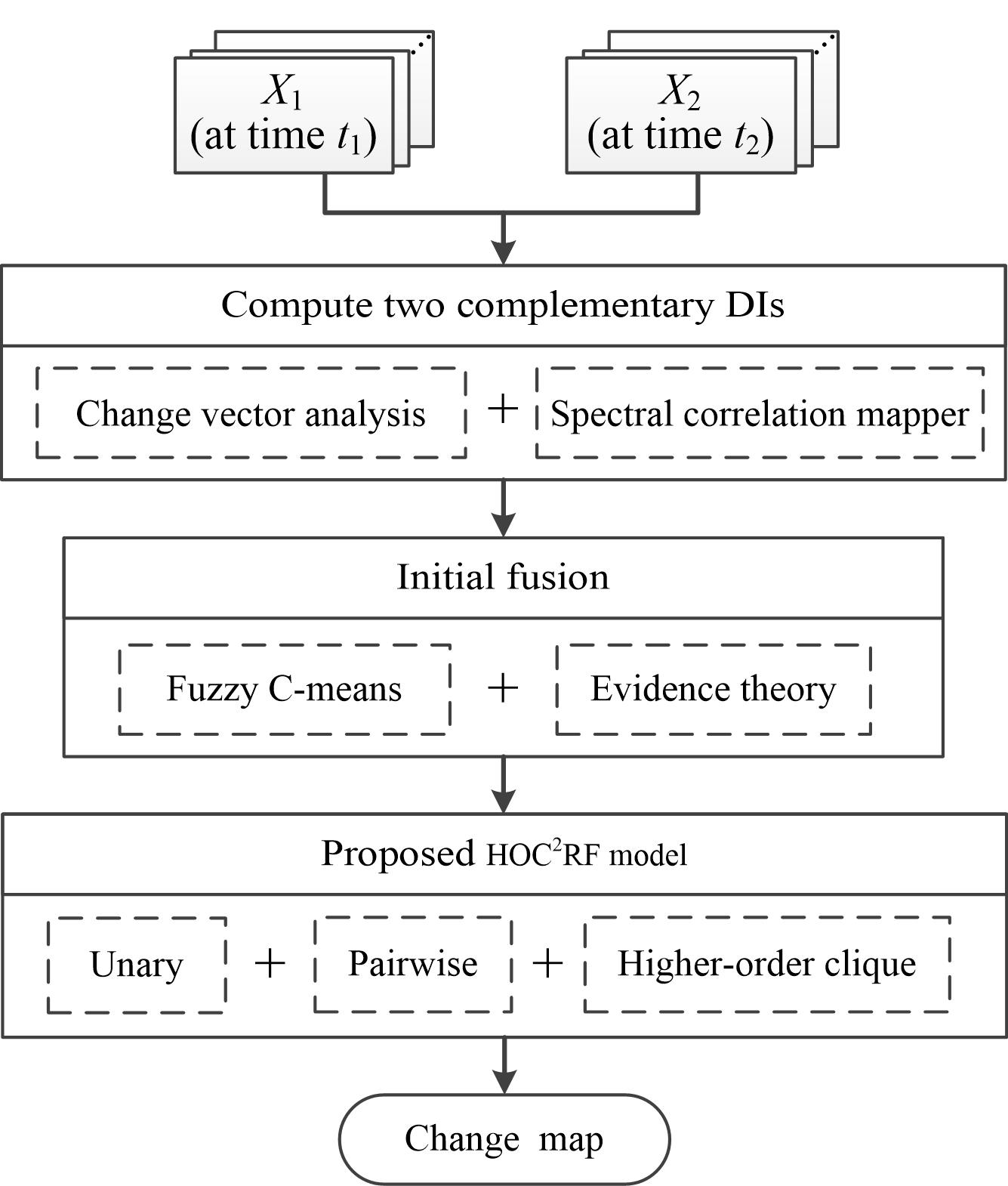
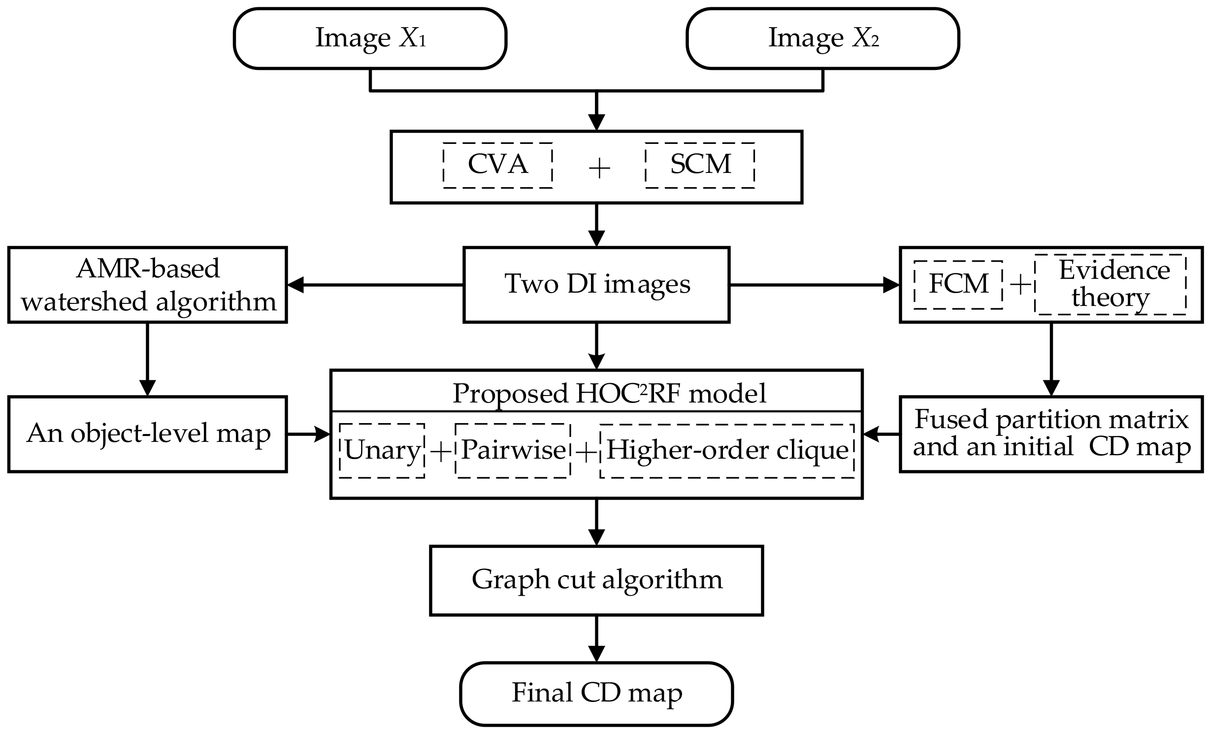
Specifically, the proposed HOC²RF CD method is achieved by the following steps (Figure 1): (1) produce two complementary DI images using CVA and SCM; (2) combine the two DIs with FCM and evidence theory to obtain the fused fuzzy partition matrix and an initial CD map; (3) generate an object-level map using the AMR-based watershed algorithm; (4) compute the unary, pairwise, and higher-order clique potentials for HOC²RF; and (5) create the final CD map by optimizing the HOC²RF model with the graph cut algorithm.

Steps 1–3 are the preparation steps for defining the HOC²RF model. The two DIs obtained in Step 1 are used to define the observation field of HOC²RF. The fused fuzzy partition matrix and initial CD map yielded in Step 2 are used to compute the unary potential and define the labeling field, respectively. The object-level map generated in Step 3 is used for computing the higher-order clique potential.

The rest of Section 3 is organized as follows: Section 3.2, Section 3.3 and Section 3.4 present the details of Steps 1–3, respectively. Section 3.5 describes the proposed HOC²RF model and its implementation in detail.

3.2. Generating Complementary DI Images

Let us consider two multispectral (or hyperspectral) remote sensing images X₁ and X₂ (with the same size of N pixels) acquired in the same geographical area at two different dates, respectively, which have been radiometrically corrected and coregistered. Both X₁ and X₂ are composed of B spectral bands (B > 1); X_tb is the bth band of image X_t, t = 1, 2; b = 1, 2, …, B.

Generally, different land cover types have their own typical spectral characteristics represented by peculiar spectral curves, although there are the phenomena of “same object with different spectrum” and “different objects with same spectrum” in some cases. Accordingly, various features could be extracted from remote sensing images. For the CD task, the differences between multitemporal remote sensing images can reflect the changes occurring on the corresponding area during the observation times to an extent, and thus can provide hints to CD. Images with multiple spectral bands can constitute spectral vectors of elements [22]. For the multispectral image CD, the DI image is generally produced based on the multitemporal spectral vectors.

However, most unsupervised CD techniques mainly take the vector magnitude change into account, failing to utilize the vector angle (or direction). The vector magnitude and angle can provide complementary change information [22], and can be described by CVA and spectral angle mapper (SAM), respectively. SAM uses cosine correlation to compute the vector angle, which is unable to detect negatively correlated data and sensitive to offset factors [27]. In contrast, SCM uses Pearson’s correlation to calculate vector angles, and can overcome the shortcomings of SAM to some extent. Given the above analysis, this study uses CVA and SCM to produce the DI images.

The DI image defined by CVA is denoted by DI_CVA. CVA uses the Euclidean distance to compute the differences between two temporal images. Specifically, DI_CVA can be computed through the following equation:

$$D{I}_{CVA}(i)=\sqrt{{\displaystyle \sum _{b=1}^B{\left(X_{2b}\right(i)-X_{1b}(i\left)\right)}^2}}$$

(1)

where X_tb(i) is the ith pixel at the bth band of image X_t, t = 1, 2; b = 1, 2, …, B; and i = 1, 2, …, N.

Denote the DI determined with SCM by DI_SCM. SCM utilizes the angle of spectral vectors to model their difference. First, the Pearson’s correlation coefficient of X₂ and X₁ is calculated by

$$\mathrm{SC}{\mathrm{M}}_i(X_2,X_1)=\frac{{\displaystyle \sum _{b=1}^B\left(X_{2b}\right(i)-{\overline{X}}_2(i\left)\right)\cdot \left(X_{1b}\right(i)-{\overline{X}}_1(i\left)\right)}}{\sqrt{{\displaystyle \sum _{b=1}^B{\left(X_{2b}\right(i)-{\overline{X}}_2(i\left)\right)}^2}}\cdot \sqrt{{\displaystyle \sum _{b=1}^B{\left(X_{1b}\right(i)-{\overline{X}}_1(i\left)\right)}^2}}}$$

(2)

where X_tb(i) denotes the ith pixel at the bth band of image X_t, and ${\overline{X}}_t(i)$ represents the average of the spectral bands of X_t at pixel i, t = 1, 2; b = 1, 2, …, B; and i = 1, 2, …, N. The correlation coefficient in (2) can be viewed as an angle if applying the arc-cosine operation to it. Thus, SCM is the centered version of SAM by ${\overline{X}}_1$ and ${\overline{X}}_2$. The SCM_i(X₂, X₁) value varies in the interval [−1, 1]. SCM_i(X₂, X₁) = 1 means that the two vectors are completely positively correlated, and SCM_i(X₂, X₁) = −1 means that the two vectors are completely negatively correlated. Then, SCM(X₂, X₁) can be converted to the DI image DI_SCM by Equation (3) or (4):

$$D{I}_{SCM}\left(i)=1-SC{M}_i\right(X_2,X_1)$$

(3)

$$D{I}_{SCM}\left(i)=\mathrm{arcos}(SC{M}_i\right(X_2,X_1\left)\right)$$

(4)

Here, X₁ and X₂ represent the two considered remote sensing images (see the beginning of this subsection). After obtaining the two DI images, their pixel values are normalized to the interval [0, 1] in order to make different datasets have the same weight.

3.3. Combine DI Images with FCM and Evidence Theory

Evidence theory (also known as Dempster-Shafer theory) [28,29] is a popular decision-level fusion framework and has been successfully applied to various applications. It can deal with both single and composite hypotheses and allows the modeling of both uncertainty and ignorance. Let us consider a frame of discernment Ω consisting of all possible single hypotheses and its power set P(Ω). A mass function for the discernment frame Ω is a mapping m from P(Ω) to the interval [0, 1] and satisfies the following properties:

$$\left\{\begin{array}{l}\mathrm{m}(\varnothing )=0\\ {\displaystyle \sum _{\mathrm{A}\in \mathrm{P}\left(\Omega \right)}m(A)=1}\end{array}\right.$$

(5)

where $\varnothing$ represents the empty set, A represents a nonempty subset of Ω, and m(A) represents the mass value of A.

In evidence theory, evidence from different sources is usually combined using the orthogonal sum. Consider D mass functions (namely, m_n, n = 1, 2, …, D) from D pieces of evidence, respectively. Their fused mass function m can be determined as follows [30]:

$$\begin{array}{l}m(A)=m_1\oplus m_2\oplus \cdots \oplus m_D\\ \hspace{0.33em}\hspace{0.33em}\hspace{0.33em}\hspace{0.33em}=\left\{\begin{array}{l}\frac{1}{1-\mathsf{\Psi }}{\displaystyle \sum _{A_1\cap \cdots \cap A_D=A}{\displaystyle \prod _{n=1}^D{m}_n(A_n) A\ne \varnothing }}\\ \hspace{0.33em}\hspace{0.33em}\hspace{0.33em}\hspace{0.33em}\hspace{0.33em}\hspace{0.33em}\hspace{0.33em}\hspace{0.33em}\hspace{0.33em}0\hspace{0.33em}\hspace{0.33em}\hspace{0.33em}\hspace{0.33em}\hspace{0.33em}\hspace{0.33em}\hspace{0.33em}\hspace{0.33em}\hspace{0.33em}A=\varnothing \end{array}\right.\end{array}$$

(6)

with

$$\mathsf{\Psi }={\displaystyle \sum _{A_1\cap \cdots \cap A_D=\varnothing }{\displaystyle \prod _{n=1}^D{m}_n\left(A_n\right)}}$$

(7)

where $\mathsf{\Psi }$ represents the degree of conflict between evidence, called the conflict coefficient.

For the CD task, there are two single hypotheses in Ω—namely, Ω = {C_u, C_c}, where C_u and C_c represent the no-change and change classes, respectively. Two pieces of evidence, the two produced DI images, are available for Ω in our case. In order to fuse the DIs with evidence theory, the first step is to define their mass functions.

Usually, there exists an overlap between the ranges of the DI pixel values from the change and no-change classes [8]. This leads to the inherent uncertainty in the analysis of DI. Fuzzy clustering provides an opportune tool for analyzing DI owning to its capability to process uncertainty. In fuzzy clustering, the pixels are not assigned to either the no-change or the change category but to both categories with a certain degree of membership. Moreover, fuzzy clustering requires no prior assumption about the distribution of the no-change and change classes. Given the above analysis, we use the popular FCM clustering to analyze the DIs for estimating their fuzzy partition matrices (also called membership functions). The mass functions for the two pieces of DI evidence are then derived from the estimated fuzzy partition matrices. The FCM details can be found in [31].

Let U_n = {u_ni(k)} represent the fuzzy partition matrix obtained by FCM based on the nth DI image, n = 1, 2, and u_ni(k) stands for the membership of the ith pixel with respect to class k, i = 1, 2, …, N; k ∈ {C_u, C_c}, satisfying

$$\left\{\begin{array}{l}0\le u_{ni}\left(k\right)\le 1\\ u_{ni}\left(C_u\right)+u_{ni}(C_c)=1\end{array}\right.$$

(8)

The mass function m_n for the nth DI image can be determined according to the fuzzy partition matrix U_n. In particular, the mass values of a given pixel i for no-change and change classes are obtained by

$$m_{ni}\left(k)=u_{ni}\right(k),\hspace{0.33em}k\in \left\{C_u,C_c\right\}$$

(9)

where m_ni(k) represents the mass value of the ith pixel to class k obtained based on the nth DI image. Then, the combined mass function m is computed through Equation (6), and an initial CD map is yielded using the principle of maximum mass value. For a given pixel i, its initial class label y_i is obtained as follows:

$$y_i=\left\{\begin{array}{l}{C}_c\hspace{0.33em}\hspace{0.33em}if\hspace{0.33em}{m}_i\left(C_c\right)\ge m_i\left(C_u\right)\\ C_u\hspace{0.33em}\hspace{0.33em}if\hspace{0.33em}{m}_i\left(C_c\right)<m_i\left(C_u\right)\end{array}\right.$$

(10)

where m_i(C_u) and m_i(C_c) represent the combined mass values of pixel i to the no-change and change classes, respectively.

3.4. Generate an Object-Level Map for HOC²RF

This subsection aims to generate an object-level map by segmenting the DI images, which will be used for computing the proposed higher-order clique potential function. Different segmentation techniques can be employed to produce object-level images, such as the spectral clustering and the seeded algorithm. Seeded segmentation algorithms have been successfully applied to many image segmentation applications because of their good performance [32]. The watershed algorithm is one of the most important seeded algorithms. However, it often suffers from the problem of over-segmentation.

This is because the watershed algorithm gains seeds from the gradient image that usually contains many seeds produced by unimportant texture details or noises. To solve this problem, an advanced AMR technique was given recently in [32] to improve the seed image. The AMR algorithm has the following advantages: (1) It is easy to implement; (2) it can remove useless seeds while maintaining meaningful ones adaptively; (3) it uses multiscale structuring elements of erosion and dilation operations and is robust to the structuring element scale; and (4) it has two attractive properties—namely, the monotonicity and the convergence, which help AMR-based algorithms obtain a hierarchical segmentation. We refer to [32] for more details of AMR.

This study proposes to use the AMR-based watershed algorithm to segment the DIs for producing an object-level map consisting of image objects. Specifically, a gradient image is created first by applying the Sobel operator to the three-dimensional DI image, DI = {DI_CVA, DI_SCM, DI_mean}, where DI_mean = (DI_CVA + DI_SCM)/2. Then, the AMR algorithm is employed to reconstruct the gradient image adaptively. Finally, the reconstructed gradient image is used as the seed image, and the watershed algorithm is adopted to yield an object-level image.

In AMR, two parameters need to be set: the scale of the minimal structuring element s and the positive threshold η used to control the convergent condition. Since the segmentation results are not sensitive to these two parameters, they are fixed in this work and set to 2 and 10⁻⁵, respectively—that is, s = 2 and η = 10⁻⁵. The obtained object-level map will be used in the next subsection for computing the higher-order potential term of the proposed HOC²RF.

3.5. HOC²RF Model

This subsection defines the proposed HOC²RF model based on the DIs, the fused fuzzy partition matrix, the initial CD map, and the object-level map obtained in Section 3.2, Section 3.3 and Section 3.4. HOC²RF integrates the complementary change information extracted from the perspective of vector magnitude and angle, and synthetically utilizes the spatial correlation of images at both the pixel and object levels. The details of the proposed HOC²RF are as follows.

Let the random variable sets X = {x₁, x₂, …, x_N} and Y = {y₁, y₂, …, y_N} denote the observation field and labeling field of an image, respectively, where N represents the total number of the pixels in the used image. x_i stands for the spectral features of pixel i, and y_i ∈ C denotes the class label of pixel i, where C = {C₁, C₂, …, C_M} is the class label set and M denotes the number of classes. For unsupervised CD, C = {C_u, C_c}.

In HOC²RF, X is defined based on the two complementary DIs, DI_CVA and DI_SCM (obtained in Section 3.2). In particular, X = DI = {DI_CVA, DI_SCM, DI_mean}, DI_mean = (DI_CVA + DI_SCM)/2, and x_i = {DI_CVA(i), DI_SCM(i), DI_mean(i)}. The initial class label y_i for the labeling field is obtained by combining DI_CVA and DI_SCM (see Section 3.3). Then, the energy function of the proposed HOC²RF is defined as follows:

$$E\left(X\right)={\displaystyle \sum _{i=1}^N{\psi }_i(y_i,X)}+\mathsf{\lambda }{\displaystyle \sum _{i=1}^N{\displaystyle \sum _{j\in N_i}{\psi }_{ij}}(y_i,y_j,X)}+{\displaystyle \sum _{o\in S}{\psi }_{high}(v_o,X)}$$

(11)

where ${\psi }_i(y_i,X),$${\psi }_{ij}(y_i,y_j,X),$ and ${\psi }_{high}(v_o,X)$ represent the unary, the pairwise, and the proposed higher-order clique potentials, respectively. N_i denotes the neighborhood of pixel I, and j ∈ N_i denotes the neighboring pixel of pixel i. In this study, the widely used second-order (i.e., the eight neighbors) neighborhood system is used to define N_i. S is the set composed of the image objects from the object-level map produced in Section 3.4, o represents an image object, v_o represents the higher-order clique of objects for o (see Equation (15)), and the parameter λ is the weight coefficient used to control the weight of the pairwise potential.

3.5.1. Unary and Pairwise Potentials

The unary potential function ${\psi }_i(y_i,X)$ is used to describe the relationship between the labeling and observation fields. ${\psi }_i(y_i,X)$ denotes the cost of pixel i taking the class label y_i given the observed data and is usually defined as the negative logarithm of the probability of pixel i belonging to class y_i:

$${\psi }_i\left(y_i,X\right)=-\log P\left(y_i\right)$$

(12)

where P(y_i) represents the probability of pixel i to class y_i, y_i ∈{C_u, C_c}, and log is the natural logarithm operator. P(y_i) can be computed with different techniques, such as FCM. In this study, P(y_i) is defined using the joint mass function that is obtained by combining the two complementary DIs DI_CVA and DI_SCM with FCM and evidence theory (see Section 3.2 and Section 3.3). This is

$$P(y_i)=\left\{\begin{array}{l}{m}_i\left(C_u\right)\hspace{0.33em}\hspace{0.33em}{y}_i=C_u\\ m_i\left(C_c\right)\hspace{0.33em}\hspace{0.33em}{y}_i=C_c\end{array}\right.$$

(13)

where m_i(C_u) and m_i(C_c) represent the combined mass values of pixel i to the no-change and change classes, respectively (see Section 3.3).

The pairwise potential function ${\psi }_{ij}(y_i,y_j,X)$ is used to utilize the spatial correlation of an image in local neighborhood, and to model the interaction between pixel i and its neighboring pixels j in N_i. It imposes a label constraint on the image by constraining the class labels to be consistent, by which the adjacent pixels with similar spectral values are encouraged to take the same class label. Following [15], the pairwise potential term in (11) is written as follows:

$${\psi }_{ij}(y_i,y_j,X)=\left\{\begin{array}{l}\hspace{0.33em}\hspace{0.33em}\hspace{0.33em}\hspace{0.33em}\hspace{0.33em}\hspace{0.33em}\hspace{0.33em}\hspace{0.33em}0 \hspace{0.33em}\hspace{0.33em}\hspace{0.33em}\hspace{0.33em}\hspace{0.33em}\hspace{0.33em}\hspace{0.33em}\hspace{0.33em}\hspace{0.33em}\hspace{0.33em}\hspace{0.33em}if\hspace{0.33em}{y}_i=y_j\hspace{0.33em}\\ 1+\exp \left(-\frac{d(x_i,x_j)}{2{\mathsf{\sigma }}^2}\right)\hspace{0.33em}\hspace{0.33em}\hspace{0.33em}\mathit{otherwise}\end{array}\right.$$

(14)

where d(x_i, x_j) is the Euclidean distance of x_i and x_j, respectively: x_i = {DI_CVA(i), DI_SCM(i), DI_mean(i)} and x_j = {DI_CVA(j), DI_SCM(j), DI_mean(j)}. ${\sigma }^2$ is the mean value of d(x_i, x_j) over the neighborhood N_i.

3.5.2. Proposed Higher-Order Clique Potential

The higher-order potential (object term) was introduced into the CD task in [21] to enhance CD performance. However, the higher-order potential in [21] only considers a single object, ignoring the dependence between neighboring objects. To overcome this shortcoming, this study proposes a novel higher-order clique potential by constructing a higher-order clique of objects and by considering the dependence between neighboring objects in both feature and location spaces. For a given object o, its higher-order clique v_o is defined as:

$$v_o=\left\{o,r^1\left(o),r^2\right(o),g^1\left(o),g^2\right(o)\right\}$$

(15)

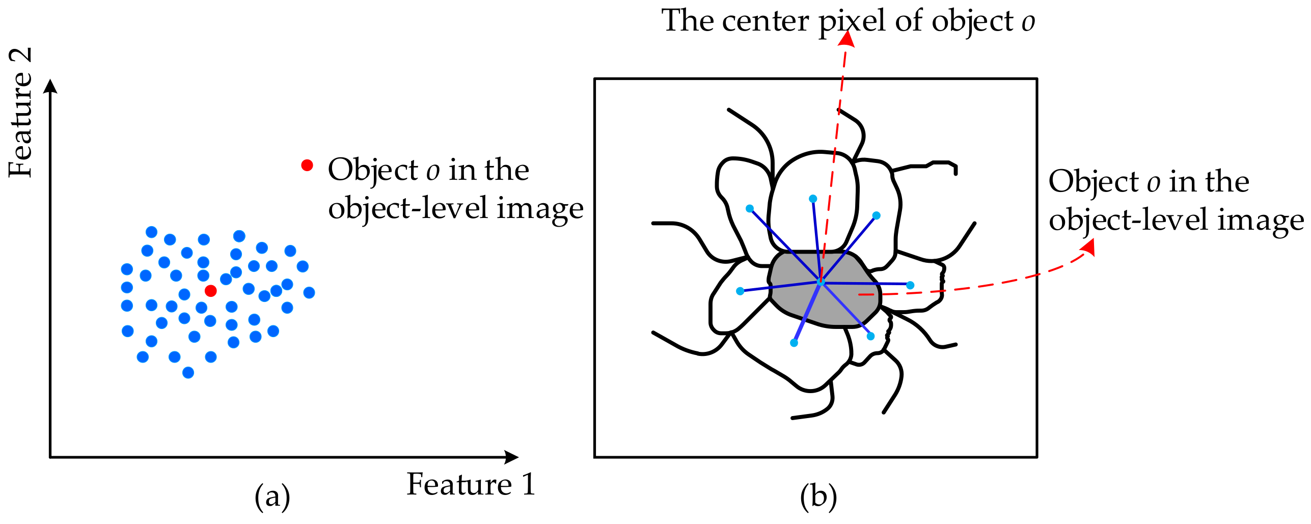
where o denotes the object o; r¹(o) and r²(o) denote the two neighboring objects that are nearest to object o in the feature space; and g¹(o) and g²(o) denote the two neighboring objects nearest to object o in the location space. Figure 2a,b shows an example of the feature space (location space) for a simple object-level image.

In order to determine the objects r¹(o), r²(o), g¹(o), and g²(o), we need to define the distances between objects in the feature and location spaces. For two given objects o¹ and o², their distance in the feature space is defined as the Euclidean distance of x(o¹) and x(o²), where x(o¹) and x(o²) denote the mean values of the DI features of the pixels in objects o¹ and o², respectively. The distance between o¹ and o² in the location space is defined as the Euclidean distance of the location coordinates of the center pixels of objects o¹ and o².

The clique v_o is made up of three parts: the object o, its two nearest neighboring objects in feature space, and its two nearest neighboring objects in location space. In general, there is correlation between the neighboring objects—in particular for the over- segmentation objects. The proposed higher-order clique potential function ${\psi }_{high}(v_o,X)$ is defined based on the object clique v_o and is used to utilize the correlation of the pixels within an object and its nearest neighboring objects in both feature and location spaces. ${\psi }_{high}(v_o,X)$ takes the following form:

$${\psi }_{high}\left(v_o,X\right)=N(v_o)\times f_o$$

(16)

where ${\psi }_{high}(v_o,X)$ is used to describe the cost of the label inconsistency in the clique v_o. N(v_o) denotes the number of the pixels in the clique v_o, and consequently, a large clique will have a large weight. $f_o$ is used to define the cost coefficient, which takes both the clique segmentation quality and the clique likelihood for change/no-change into account. In particular, the cost coefficient $f_o$ is defined as:

$$f_o=\min \left\{\underset{k}{\min }\left(q\left(v_o\right)\times z^k\left(v_o)+(1-z^k\right(v_o\left)\right)\right), 1\right\}$$

(17)

where min represents the minimum operator, q(v_o) represents the clique segmentation quality of clique v_o, and z^k(v_o) represents the clique likelihood of clique v_o to class k, k∈{C_u, C_c}.

In this study, the clique segmentation quality, q(v_o), is defined as the weighted average sum of the segmentation quality of the objects in clique v_o:

$$q(v_o)=\frac{q(o)+0.5q(r^1(\mathsf{o}))+0.5q(r^2(\mathsf{o}))+0.5q(g^1(\mathsf{o}))+0.5q(g^2(\mathsf{o}))}{1+4\times 0.5}$$

(18)

where q(o), q(r¹(o)), q(r²(o)), q(g¹(o)), and q(g²(o)) stand for the segmentation quality of objects o, r¹(o), r²(o), g¹(o), and g²(o), respectively.

Let o^l denote a given object in clique v_o. Then, the object segmentation quality of o^l is estimated based on the object consistency assumption, which encourages all the pixels in an object to have the same class label. Specifically, we define q(o^l) as follows: q(o^l) = (N(o^l) − N_k(o^l))/Q(o^l), where N(o^l) denotes the number of the pixels in object o^l, N_k(o^l) denotes the number of the pixels assigned to class k in object o^l, k∈{C_u, C_c}, and Q(o^l) denotes a truncated parameter used to adjust the degree of rigidity of q(o^l). This study sets Q(o^l) = 0.1 × N(o^l). That means, if more than 90% of the pixels in o^l are assigned to C_c or C_u, the value of q(o^l) is less than 1. Similarly, if 70% of the pixels in object o^l are assigned to C_c or C_u, the value of q(o^l) is set to 3.

According to the definition of q(o^l), the more pixels of an object have the same class label, the better segmentation quality on this object and the smaller value of q(o^l) will be. As a result, the better the segmentation quality of the objects in clique v_o is, the smaller value of q(v_o) will be (see Equation (18)).

The clique likelihood z^k(v_o) is defined based on the number of pixels in the objects from clique v_o and the objects’ joint mass values, taking the following form:

$$z^k(v_o)=\frac{N\left(o\right)\times m^k\left(o)+0.5N\right(r^1(o\left)\right)\times m^k(r^1\left(o\left)\right)+0.5N\right(r^2(o\left)\right)\times m^k(r^2\left(o\left)\right)+0.5N\right(g^1(o\left)\right)\times m^k(g^1\left(o\left)\right)+0.5N\right(g^2(o\left)\right)\times m^k(g^2(o\left)\right)}{N\left(o)+0.5N\right(r^1\left(o\left)\right)+0.5N\right(r^2\left(o\left)\right)+0.5N\right(g^1\left(o\left)\right)+0.5N\right(g^2(o\left)\right)}$$

(19)

where N(o), N(r¹(o)), N(r²(o)), N(g¹(o)), and N(g²(o)) denote the number of the pixels in objects o, r¹(o), r²(o), g¹(o), and g²(o), respectively. m^k(o) denotes the joint mass value of the object o to class k and is computed via m^k(o) = ${\displaystyle {\sum }_{i\in o}{m}_i}(k)/N(o)$, where m_i(k) denotes the joint mass value of pixel i to class k, k∈{C_u, C_c}. m^k(r¹(o)), m^k(r²(o)), m^k(g¹(o)), and m^k(g²(o)) have the similar definition of m^k(o).

Generally, the center object in clique v_o is more important than their neighboring objects. Accordingly, when computing q(v_o) and z^k(v_o), the weight of object o is set to 1, whereas the weights of objects r¹(o), r²(o), g¹(o), and g²(o) are set to 0.5.

On the one hand, the proposed higher-order clique potential encourages all pixels in clique v_o to have the same class label. On the other hand, it uses the label consistency in a clique as a soft constraint and, thus, enables some pixels in the clique to take different labels. Accordingly, the higher-order clique potential can make effective use of the interaction of the pixels within an object and its nearest neighboring objects in both feature and location spaces and, thus, can improve the CD performance.

Different optimization algorithms, such as graph cuts and iterated conditional modes, can be adopted to minimize (optimize) the CRF model. The graph cut algorithm [33] is used to minimize the HOC²RF model for producing the final CD map.

4. Results

This section evaluates the performance of the proposed HOC²RF CD method. To this end, experiments were conducted on three real remote sensing datasets acquired by different sensors. Before performing CD, the relative radiometric correction and co-registration have been done on the three datasets, in order to make the two-temporal remote sensing images of each dataset to be comparable in both spectral and spatial spaces.

4.1. Dataset Description and Experimental Settings

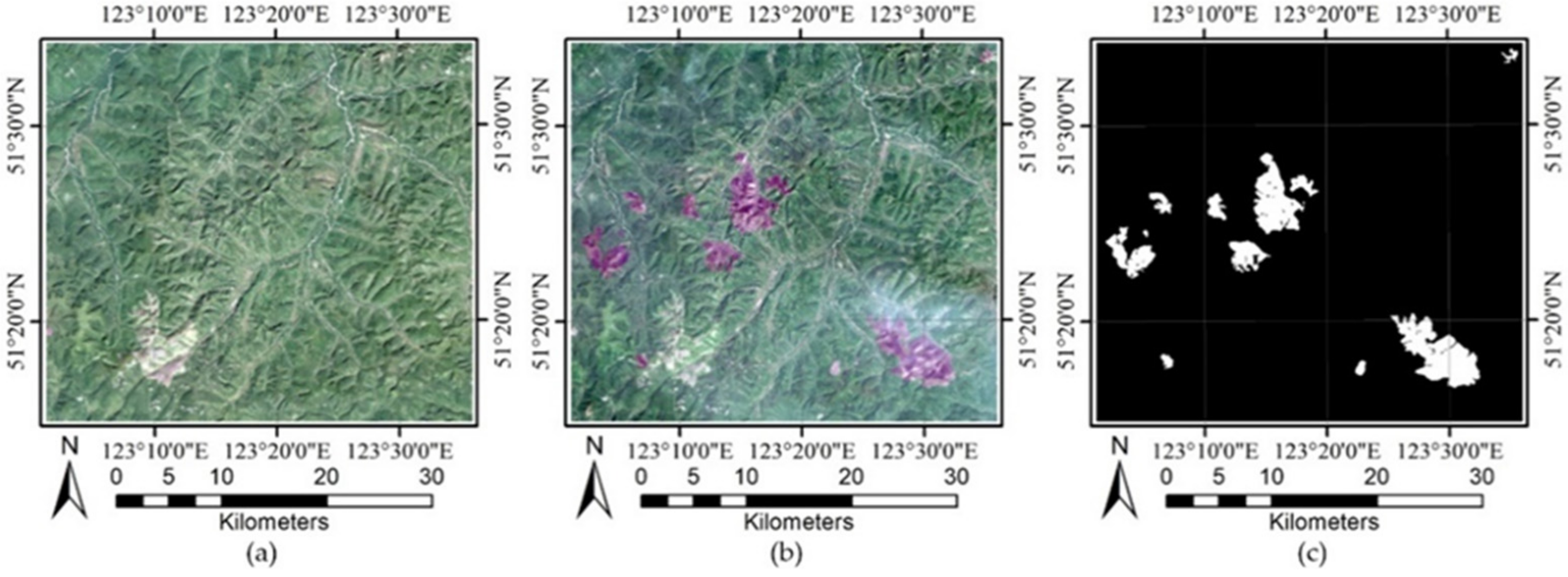
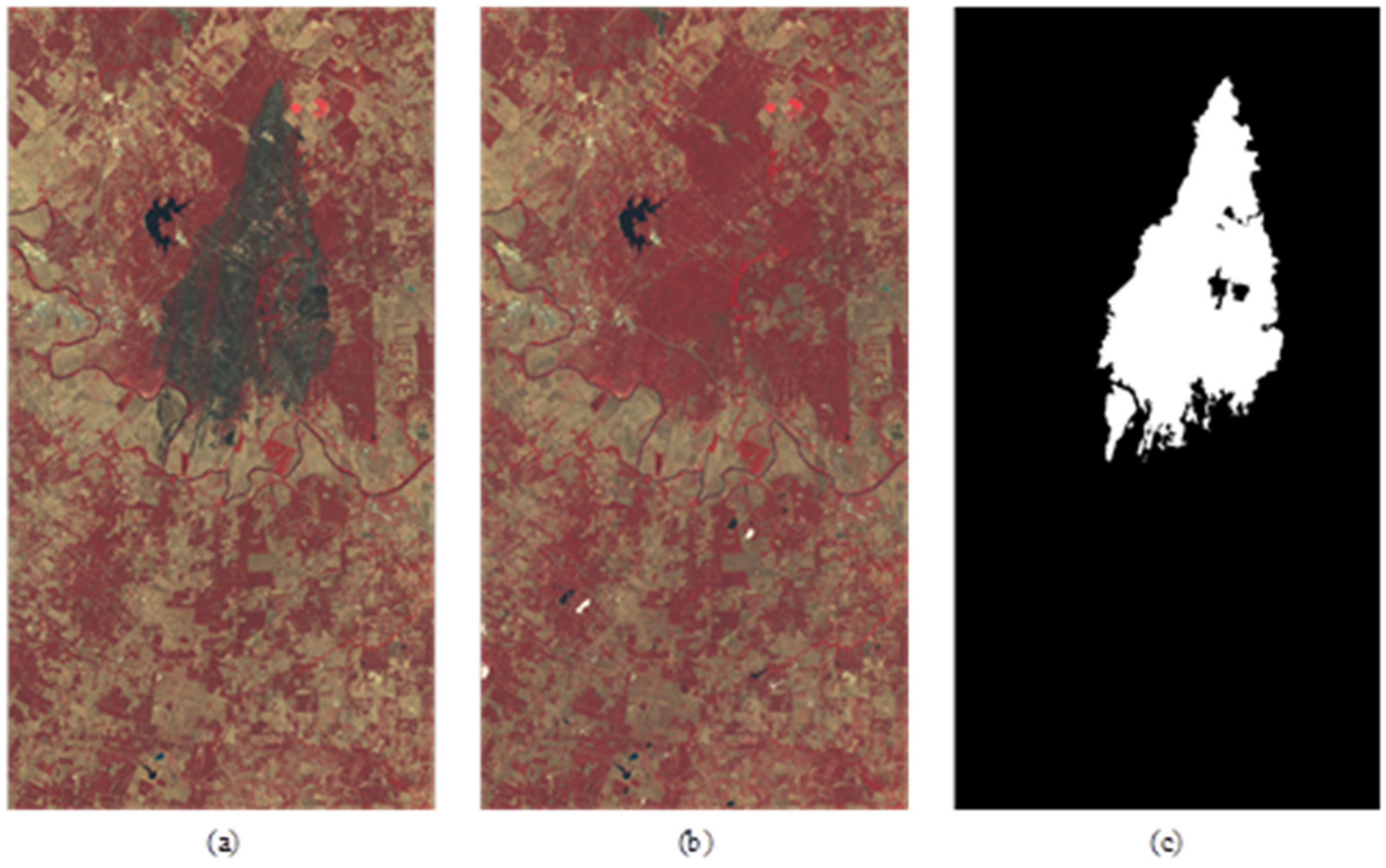
The first experiment was conducted on the Neimeng dataset, which comprises a pair of multispectral images taken by Landsat-5 Thematic Mapper sensor on 22 August 2006 and 17 June 2011 in the boundary area between the Neimeng and Heilongjiang Provinces, China. This dataset covers an area with 1200 × 1350 pixels, and contains one main type of land cover, forest. The changes occurred in this study area mainly due to a wildfire. Bands 1, 2, 3, 4, 5, and 7 were used for CD. Figure 3a–c shows the images of 2006 and 2011, and their reference map, respectively. The reference map was produced according to a careful visual interpretation of the two-temporal images.

The second dataset, the Texas dataset, consists of two multispectral images with 1534 × 808 pixels acquired by Landsat-5 Thematic Mapper sensor on August 26 and September 11, 2011. The dataset covers a forest fire in Bastrop County, Texas. Bands 1, 2, 3, 4, and 5 were used for CD. Figure 4a–c shows the images of August and September, and their reference map, respectively.

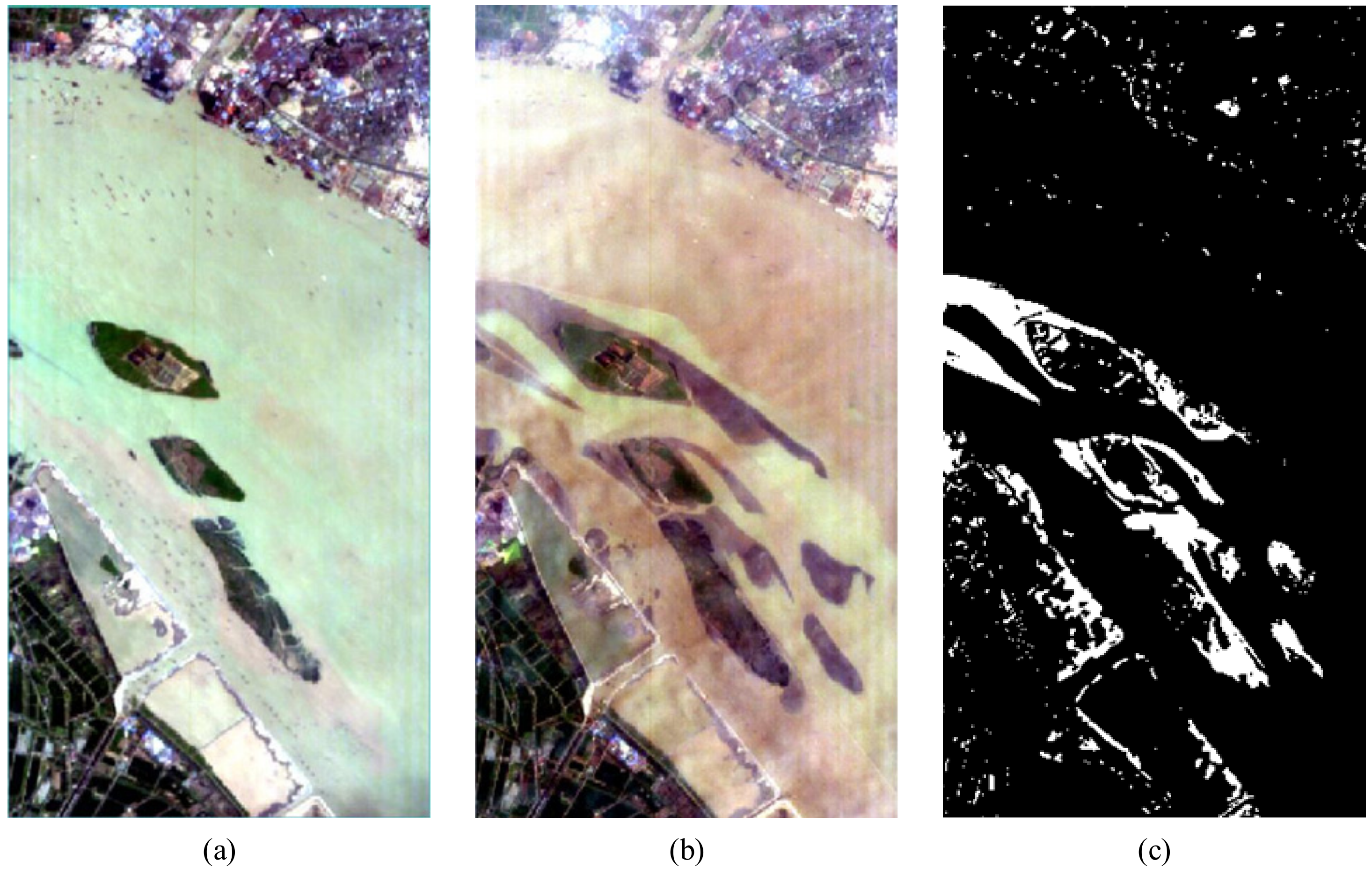
The third dataset is the Poyang River dataset (463 × 241 pixels), which is made up of two Earth Observing-1 (EO-1) Hyperion images acquired on 3 May 2013 and 31 December 2013, respectively, in Jiangsu province, China. The dataset has 198 bands available after noisy band removal. The images of May and December are displayed in Figure 5a,b, respectively; and their reference map is shown in Figure 5c.

The Texas and Poyang River datasets are provided by [34,35], respectively. These two datasets are both offered in MAT format, and their location information is unavailable. As a result, we cannot show the information regarding the north direction and detailed location for these two datasets (Figure 4 and Figure 5).

To assess the effectiveness of the proposed HOC²RF CD method, it was compared with nine related approaches, CVA, SCM, the reformulated fuzzy local information C-means (RFLICM) [36], MRF [3], the traditional pairwise CRF (CRF), the fully-connected CRF (FCCRF) [37], the improved FCCRF (IFCCRF) [17], the higher-order CRF (HOCRF) [21], and the improved nonlocal patch-based graph (INLPG) [38].

Seven measures [39] were employed to conduct the performance evaluation: false positives (FP), the number of the unchanged pixels that are wrongly detected as changed ones; false negatives (FN), the number of the changed pixels that are wrongly detected as unchanged ones; true positives (TP), the number of the correctly detected change pixels; true negatives (TN), the correctly detected no-change pixels; overall errors (OE), the sum of FP and FN, OE = FP + FN; the overall accuracy (OA), OA = 1 − OE/(TP + TN + FP + FN); and the Kappa coefficient (KC), which is calculated by

$$\mathrm{KC}=\frac{N\times (\mathrm{TP}+\mathrm{TN})-\left(\right(\mathrm{TN}+\mathrm{FN})\times (\mathrm{TN}+\mathrm{FP})+(\mathrm{TP}+\mathrm{FP})\times (\mathrm{TP}+\mathrm{FN}))}{N^2-\left(\right(\mathrm{TN}+\mathrm{FN})\times (\mathrm{TN}+\mathrm{FP})+(\mathrm{TP}+\mathrm{FP})\times (\mathrm{TP}+\mathrm{FN}))}$$

(20)

For the CD task, FP and FN are also known as false alarms (FA) and missed detections (MD), respectively. FA and MD are more widely used than FP and FN in CD literature. KC involves more classification information, and thus it is more cogent than the other indicators [39].

In addition, the consumption time of each algorithm is also an important criterion. It was recorded for the comparison of time complexity of different algorithms. The nine comparative methods and the proposed HOC²RF were all conducted in a computer with Intel(R) Core(TM) i7-9750H 2.59 GHz processor and 16 GB RAM.

The parameter m used in FCM and RFLICM to adjust the fuzzy degree of membership was set to 2. The other parameters used in the compared and our algorithms were obtained by experiments, and only the results with the best parameters were given for performance assessment. For the Neimeng, Texas, and Poyang River datasets, the weights of the pairwise potentials about MRF, CRF, HOCRF and the proposed HOC²RF were set to 4/7/3, 5/8/2, 5/7/1, and 8/9/1, respectively.

The weights of the higher-order potential of HOCRF [21] were set to 3, 2 and 1. For our method, there is no need to set the weight of the higher-order clique potential, which is a fixed value, 1 (see Equation (11)). There are five parameters in FCCRF and IFCCRF: the two weights of the Gaussian kernels (w₁ and w₂), and the control parameters of nearness, similarity, and smoothness (θ_α, θ_β, and θ_γ). The same as the two weights, the three control parameters, θ_α, θ_β, and θ_γ, are also dimensionless. The values of the parameters in FCCRF and IFCCRF used in the experiments are shown in

Table 2. The values of the parameters of FCCRF and IFCCRF used in the experiments.

Dataset	Method	w1	w2	${\mathit{\theta }}_{\mathit{\alpha }}$	${\mathit{\theta }}_{\mathit{\beta }}$	${\mathit{\theta }}_{\mathit{\gamma }}$
Neimeng	FCCRF	8	4	80	10	30
	IFCCRF	2	1	50	50	80
Texas	FCCRF	6	1	5	20	20
	IFCCRF	3	1	30	5	40
Poyang River	FCCRF	1	1	80	10	10
	IFCCRF	1	1	10	80	10

.

4.2. Result and Analysis

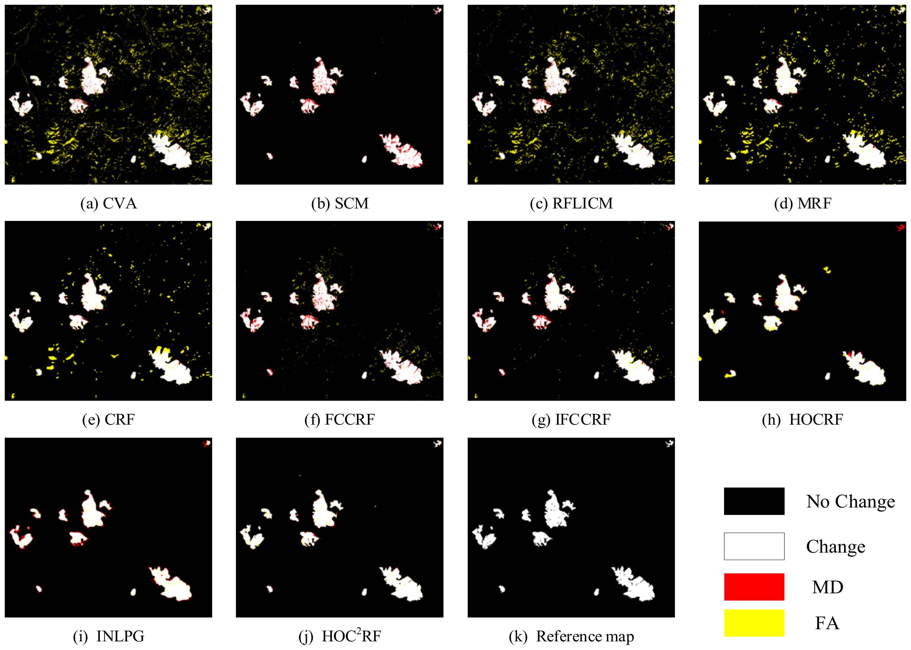
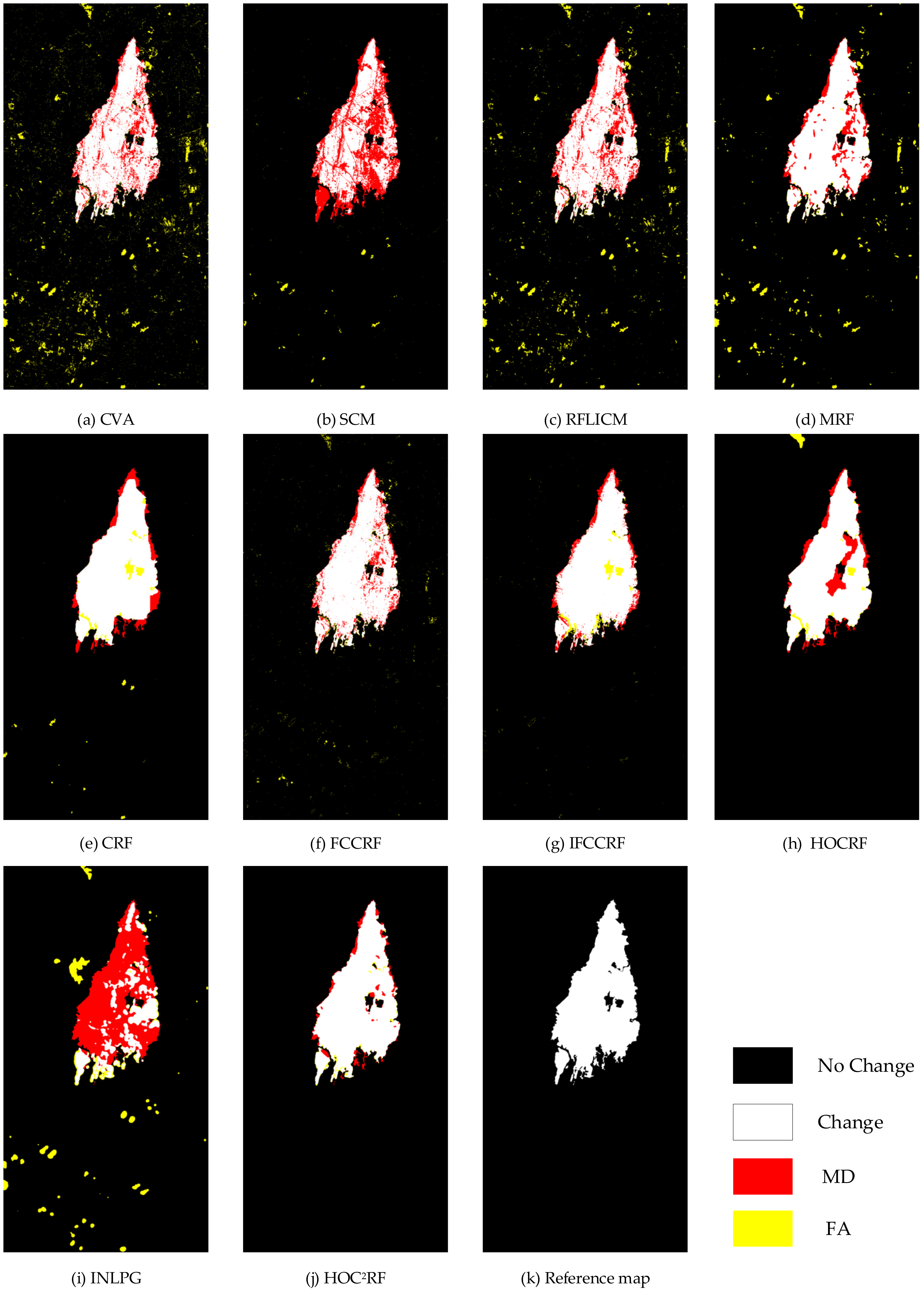
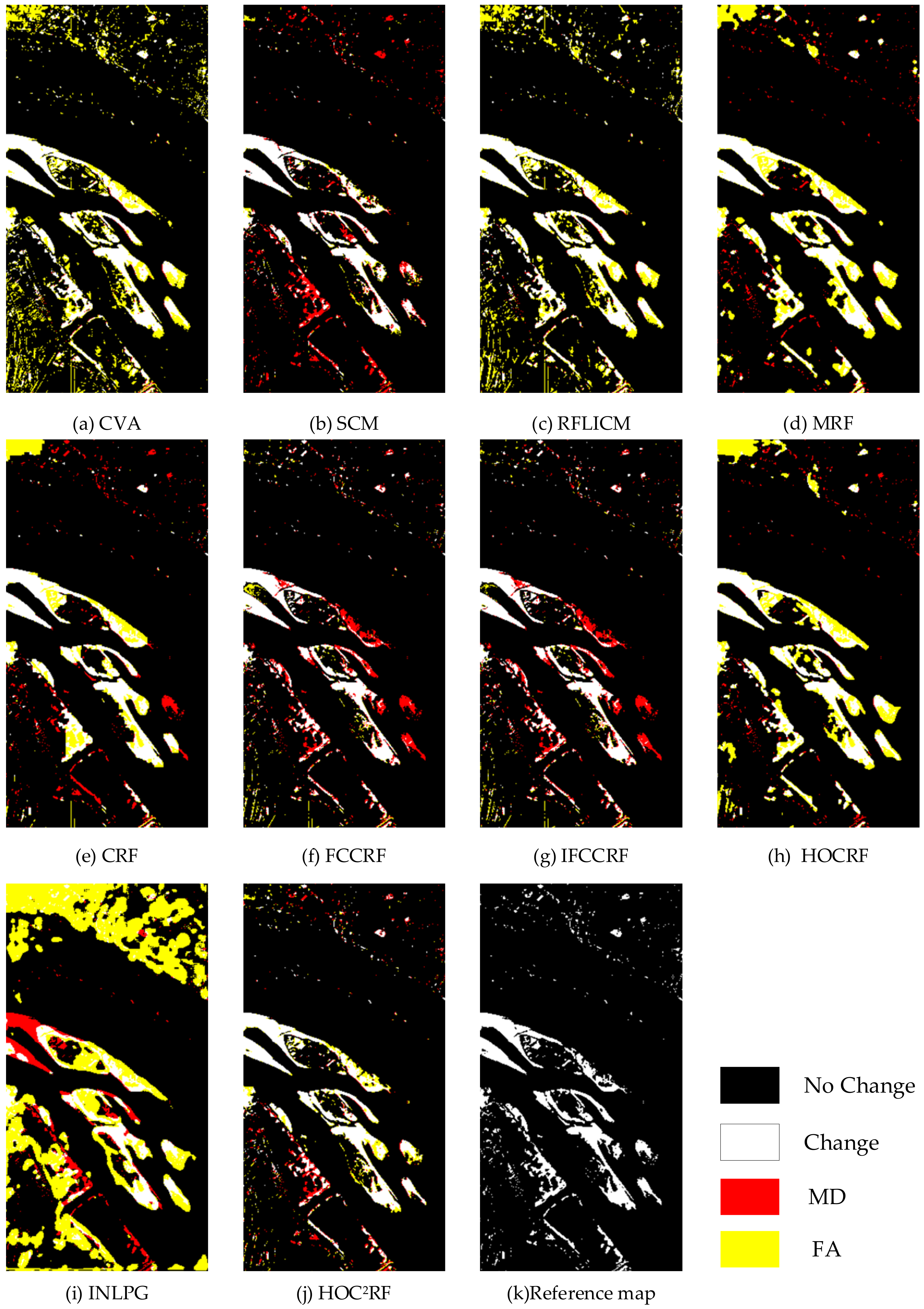
The CD results in this study are presented in two ways: the CD maps in a graphical format and the quantitative indicators in a tabular format. Figure 6, Figure 7 and Figure 8 demonstrate the CD maps of different methods on the three datasets: (a)–(j) were produced by CVA, SCM, RFLICM, MRF, CRF, FCCRF, IFCCRF, HOCRF, INLPG, and the proposed HOC²RF approach, respectively. Black stands for the correctly detected no-change pixels, white stands for the correctly detected change pixels, red stands for the MD pixels, whereas yellow stands for the FA pixels.

Table 3. Quantitative indicators for CD maps on the Neimeng dataset.

Methods	MD	FA	TP	TN	OE	OA	KC	Time(s)
CVA	3400	877,835	77,790	1,450,975	91,235	0.9437	0.6037	10.39
SCM	12,280	1174	68,910	1,537,636	13,454	0.9917	0.9067	3.30
RFLICM	4356	53,102	76,834	1,485,708	57,458	0.9645	0.7099	37.94
MRF	2255	43,478	78,935	1,495,332	45,788	0.9718	0.7610	11.90
CRF	2384	24,634	78,806	1,514,176	27,018	0.9833	0.8450	14.85
FCCRF	10,425	9261	70,765	1,529,549	19,686	0.9878	0.8715	4.33
IFCCRF	7970	7362	73,220	1,531,448	15,332	0.9905	0.9002	7.22
HOCRF	4027	8375	77,163	1,530,435	12,402	0.9923	0.9216	21.62
INPLG	9557	2701	71,633	1,536,109	12,258	0.9924	0.9172	4058.78
HOC2RF	2181	3164	79,009	1,535,646	5345	0.9967	0.9655	26.93

,

Table 4. Quantitative indicators for CD maps on the Texas dataset.

Methods	MD	FA	TP	TN	OE	OA	KC	Time(s)
CVA	24,823	31,056	107,046	1,076,547	55,879	0.9549	0.7677	4.86
SCM	59,124	2648	72,745	1,104,955	61,772	0.9502	0.6770	2.53
RFLICM	27,531	20,366	104,338	1,087,237	47,897	0.9614	0.7918	26.56
MRF	18,097	14,788	113,772	1,092,815	32,885	0.9735	0.8589	9.11
CRF	14,124	6457	117,745	1,101,146	20,581	0.9834	0.9104	8.01
FCCRF	16,890	5515	114,979	1,102,088	22,405	0.9819	0.9012	2.28
IFCCRF	12,338	6449	119,531	1,101,154	18,787	0.9848	0.9187	7.02
HOCRF	18,197	5053	113,672	1,102,550	23,250	0.9812	0.8968	15.00
INPLG	92,221	19,771	39,648	1,087,832	111,992	0.9096	0.3731	3553.57
HOC2RF	8664	2472	123,205	1,105,131	11,136	0.9910	0.9518	20.96

and

Table 5. Quantitative indicators for CD maps on the Poyang River dataset.

Methods	MD	FA	TP	TN	OE	OA	KC	Time(s)
CVA	347	8286	9351	93,599	8633	0.9226	0.6443	0.63
SCM	3169	930	6529	100,955	4099	0.9633	0.7416	0.62
RFLICM	434	6581	9264	95,304	7015	0.9371	0.6922	2.07
MRF	1222	6182	8476	95,703	7404	0.9336	0.6605	0.71
CRF	2144	3787	7554	98,098	5931	0.9468	0.6889	0.92
FCCRF	3479	945	6219	100,940	4424	0.9604	0.7167	0.23
IFCCRF	3489	862	6209	101,023	4351	0.9610	0.7200	1.81
HOCRF	1105	6244	8593	95,641	7349	0.9341	0.6653	3.54
INPLG	3840	23,738	5858	78,147	27,578	0.7528	0.1924	1317.21
HOC2RF	1727	2168	7971	99,717	3895	0.9651	0.7845	4.94

list the quantitative indicators of different CD maps for the three datasets: The unit of time is the second (s), and the other indicators are dimensionless.

As shown in Figure 6, Figure 7 and Figure 8, CVA and SCM provide complementary CD maps for all three datasets: The change maps obtained by CVA contain a large number of FA errors (yellow areas) but a small amount of MD errors (red areas), whereas the maps generated by SCM have small yellow FA areas but large red areas of MD (Figure 6a,b, Figure 7a,b and Figure 8a,b). This observation proves that CVA and SCM can yield complementary change information and shows the potentials to enhance the CD performance by performing fusion strategies.

In terms of the other seven comparative algorithms, for the Neimeng dataset, HOCRF and INLPG yield better CD results than RFLICM, MRF, CRF, FCCRF, and IFCCRF (Figure 6c–i and Table 3). However, the map of HOCRF still contains a few apparent yellow FA errors, whereas the INLPG’s map includes some apparent red MD areas. For the Texas dataset, CRF and IFCCRF generate better CD results than other comparative methods (Figure 7c–i and Table 4).

However, some obvious red MD errors still exist at the boundary of the change regions in their CD maps (Figure 7e,g). For the Poyang River dataset, FCCRF and IFCCRF perform better than RFLICM, MRF, CRF, HOCRF, and INLPG (Figure 8c–i and Table 5). Nevertheless, the maps of FCCRF and IFCCRF have many MD errors.

By integrating FCM, evidence theory, and the novel higher-order clique CRF model (developed in this study), the proposed HOC²RF CD approach first combines the complementary change information coming from the perspective of vector magnitude and angle (direction) and then utilizes the spatial correlation of images at both pixel and object levels to enhance the performance of CD. HOC²RF performs better than the nine benchmark algorithms and produces the most accurate change maps for all the three datasets (Figure 6, Figure 7 and Figure 8).

Table 3, Table 4 and Table 5 demonstrate the quantitative superiority of the proposed HOC²RF CD method. It yields the lowest OE and highest KC for all three datasets. For example, for the Neimeng dataset, its KC value is 0.9655, which is 36.18%, 5.88%, 25.56%, 20.45%, 12.05%, 9.4%, 6.53%, 4.39%, and 4.83% larger than CVA, SCM, RFLICM, MRF, CRF, FCCRF, IFCCRF, HOCRF, and INLPG, respectively. For the Texas dataset, its OE is 11136 pixels, which decreases by at least 7600 pixels in compaction to the nine alternative methods.

For the computation time complexity, INPLG takes much more time than the other methods as it has a complex process of generating DIs. The proposed HOC²RF has slightly higher computation time requirement than the CVA, SCM, MRF, CRF, FCCRF, IFCCRF, and HOCRF. For RFLICM, it takes more time than our method for the first two datasets but less time for the third dataset.

5. Discussion

5.1. Enhancing Process of HOC²RF

As shown in Table 3, Table 4 and Table 5, for all the three datasets, the proposed HOC²RF method outperforms the nine benchmark methods over both OE and KC. Furthermore, the similar results for the three datasets demonstrate the robustness of HOC²RF to some extent.

In this subsection, the Neimeng and Texas datasets are taken as examples to analyze and discuss the enhancing process of HOC²RF. To this end,

Table 6. CD results obtained by evidence theory, SHOC²RF, CVA-HOC²RF and HOC²RF.

Methods	Neimeng				Texas
	MD	FA	OE	KC	MD	FA	OE	KC
Evidence	5967	11,375	17,342	0.8910	29,200	6974	36,174	0.8342
SHOC2RF	1213	9436	10,649	0.9341	17,722	1738	19,460	0.9128
CVA-HOC2RF	2497	9104	11,601	0.9276	14,908	1600	16,508	0.9267
HOC2RF	2181	3164	5345	0.9655	8664	2472	11,136	0.9518

demonstrates the CD results produced by evidence theory, SHOC²RF, CVA-HOC²RF and the proposed HOC²RF. The CD results of evidence theory were obtained by combining the ones of CVA and SCM with evidence theory. SHOC²RF and CVA-HOC²RF can be viewed as two special cases of HOC²RF, which are used to analyze the effects of using the higher-order clique potential (16) and using the two complementary DIs, respectively. In SHOC²RF, the higher-order clique potential (16) is replaced with the higher-order potential (object term) in [21]. CVA-HOC²RF only uses the DI produced by CVA, removing the DI from SCM.

Through comparing the CD results generated by CVA, SCM, evidence theory, and the proposed HOC²RF in Table 3, Table 4 and Table 6, it can be seen that HOC²RF enhances the CD performance by two stages:

(1) Combining the CD results from CVA and SCM using evidence theory. For the Neimeng dataset, the CD results of the evidence theory are better than those of CVA, RFLICM, MRF, CRF, and FCCRF, which use only one DI (Table 3 and Table 6). For the Texas dataset, evidence theory performs better than CVA, SCM, and RFLICM (Table 4 and Table 6). Although the evidence theory’s CD results are slightly worse than those from SCM for Neimeng dataset, the FA errors of CVA and the MD errors of SCM are both significantly reduced by the fusion step. This results in more balanced FA and MD errors in the CD result of evidence theory, and thus makes it easier to further improve the performance of CD by using the CRF model. In addition, the advantages of using two complementary DIs also can be seen by comparing the CD results of CVA-HOC²RF and HOC²RF (Table 6). HOC²RF that fuses two DIs from CVA and SCM produces much better CD results than CVA-HOC²RF that only uses the CVA DI. For example, for the Neimeng dataset, the value of KC increases from 0.9276 for CVA-HOC²RF to 0.9655 for HOC²RF.

(2) Improving the fused CD results of evidence theory by utilizing the HOC²RF model. For both Neimeng and Texas datasets, HOC²RF outperforms MRF, CRF, FCCRF, IFCCRF, and HOCRF (Table 3, Table 4 and Table 6), demonstrating the superiority of the HOC²RF model. In addition, by comparing the SHOC²RF and HOC²RF rows in Table 6, we can see that, the proposed higher-order clique potential (16) performs much better than the higher-order potential used in [21]. For instance, for the Texas dataset, the KC value increases from 0.9128 for SHOC²RF to 0.9518 for HOC²RF. This is mainly because the higher-order potential in [21] only considers a single object, ignoring the dependence of the neighboring objects, whereas the proposed higher-order clique potential (16) uses an object clique consisting of an object and its neighboring objects in both feature and location spaces.

5.2. Parameter Comparison of Random Field Models

This subsection compares the parameters used in MRF, CRF, FCCRF, IFCCRF, HOCRF, and the proposed HOC²RF. Only one parameter (λ) needs to be set for implementing of the proposed HOC²RF, the same as MRF and the traditional pairwise CRF. The parameter λ is used to tune the weight of the pairwise potential. In general, a small λ causes low MD errors but leads to a large amount of noise, whereas a large one will remove some noise but may miss some detailed changes. For HOCRF [21], it needs to set two parameters, the weights of the pairwise potential and higher-order potential (object term). For both FCCRF and IFCCRF, there are five parameters to be set: the two weights of the Gaussian kernels (w₁ and w₂), and the control parameters of nearness, similarity, and smoothness (θ_α, θ_β, and θ_γ). Given the above analysis, the proposed HOC²RF needs much less parameter tuning than FCCRF IFCCRF, and HOCRF.

6. Conclusions

In this paper, a novel, unsupervised CD method was proposed by developing a higher-order clique CRF model, termed HOC²RF. For the observation field, HOC²RF further introduces the vector angle change of two temporal images compared with the existing CRF-based CD methods, which mainly utilize the vector magnitude change. For the labeling field, HOC²RF uses FCM and evidence theory to fuse the two complementary types of change information at the decision level to create an initial CD map.

Moreover, HOC²RF defines a novel higher-order clique potential based on a properly designed clique of objects. The clique potential considers the interactions between neighboring objects in both feature and location spaces. As a consequence, HOC²RF can combine the complementary change information coming from the perspective of vector magnitude and angle and utilize the spatial-context information of images at both the pixel and object levels effectively.

Three case studies verified the effectiveness and advantages of the proposed HOC²RF approach. The Kappa coefficient/overall accuracy values of HOC²RF were 0.9655/0.9967, 0.9518/0.9910, and 0.7845/0.9651, respectively, which are better than the nine benchmark methods (CVA, SCM, RFLICM, MRF, CRF, FCCRF, IFCCRF, HOCRF, and INLPG). For example, the Kappa coefficient values of HOC²RF increased at least by 4.39%, 3.31%, and 4.29% compared to the nine methods.

HOC²RF has only one parameter, thereby, needing much less parameter tuning compared with HOCRF, FCCRF, and IFCCRF. Theoretically, this article contributes to CD development by proposing the idea of using the interaction between neighboring objects in both feature and location spaces to enhance the CD performance. Methodologically, we presented a method to construct a higher-order clique, developed a higher-order clique potential function, and proposed a novel CD method—HOC²RF.

The proposed method has two limitations: (1) It has a slightly higher computation time requirement than the existing CRF CD methods because it needs to combine two DI images and compute the higher-order clique potential function. (2) Though it has only one parameter, it still requires parameter tuning.

Future work can focus on the following two directions. (1) To further automate HOC²RF, additional work can be conducted on the automatic determination of the only parameter λ used in HOC²RF. (2) Additional research can be conducted on how to define new higher-order clique potential functions.

References

- Hussain, M.; Chen, D.; Cheng, A.; Wei, H.; Stanley, D. Change detection from remotely sensed images: From pixel-based to object-based approaches. ISPRS J. Photogramm. Remote Sens. 2013, 80, 91–106. [Google Scholar] [CrossRef]
- Lv, Z.; Liu, T.; Benediktsson, J.A.; Falco, N. Land cover change detection Techniques: Very-high-resolution optical Images: A review. IEEE Geosci. Remote Sens. Mag. 2022, 10, 44–63. [Google Scholar] [CrossRef]
- Bruzzone, L.; Prieto, D.F. Automatic analysis of the difference image for unsupervised change detection. IEEE Tran. Geosci. Remote Sens. 2000, 38, 1171–1182. [Google Scholar] [CrossRef] [Green Version]
- Hao, M.; Zhou, M.; Jin, J.; Shi, W. An advanced superpixel-based markov random field model for unsupervised change detection. IEEE Geosci. Remote Sens. Lett. 2019, 17, 1401–1405. [Google Scholar] [CrossRef]
- Shao, P.; Shi, W.; Liu, Z.; Dong, T. Unsupervised change detection using fuzzy topology-based majority voting. Remote Sens. 2021, 13, 3171. [Google Scholar] [CrossRef]
- Patra, S.; Ghosh, S.; Ghosh, A. Histogram thresholding for unsupervised change detection of remote sensing images. Int. J. Remote Sens. 2011, 32, 6071–6089. [Google Scholar] [CrossRef]
- Shao, P.; Shi, W.Z.; He, P.F.; Hao, M.; Zhang, X.K. Novel approach to unsupervised change detection based on a robust semi-supervised FCM clustering algorithm. Remote Sens. 2016, 8, 264. [Google Scholar] [CrossRef] [Green Version]
- Ghosh, A.; Mishra, N.S.; Ghosh, S. Fuzzy clustering algorithms for unsupervised change detection in remote sensing images. Inf. Sci. 2011, 181, 699–715. [Google Scholar] [CrossRef]
- Du, P.J.; Liu, S.C.; Gamba, P.; Tan, K.; Xia, J.S. Fusion of difference images for change detection over urban areas. IEEE J. Sel. Top. Appl. Obs. Earth Remote Sens. 2012, 5, 1076–1086. [Google Scholar] [CrossRef]
- Celik, T. Unsupervised change detection in satellite images using principal component analysis and k-means clustering. IEEE Geosci. Remote Sens. Lett. 2009, 6, 772–776. [Google Scholar] [CrossRef]
- Lv, Z.; Liu, T.; Shi, C.; Benediktsson, J.A. Local histogram-based analysis for detecting land cover change using VHR remote sensing images. IEEE Geosci. Remote Sens. Lett. 2021, 18, 1284–1287. [Google Scholar] [CrossRef]
- Bazi, Y.; Melgani, F.; Al-Sharari, H.D. Unsupervised change detection in multispectral remotely sensed imagery with level set methods. IEEE Trans. Geosci. Remote Sens. 2010, 48, 3178–3187. [Google Scholar] [CrossRef]
- Hao, M.; Zhang, H.; Shi, W.; Deng, K. Unsupervised change detection using fuzzy c-means and MRF from remotely sensed images. Remote Sens. Lett. 2013, 4, 1185–1194. [Google Scholar] [CrossRef]
- Hedjam, R.; Kalacska, M.; Mignotte, M.; Nafchi, H.Z.; Cheriet, M. Iterative classifiers combination model for change detection in remote sensing imagery. IEEE Trans. Geosci. Remote Sens. 2016, 54, 6997–7008. [Google Scholar] [CrossRef]
- Lv, P.; Zhong, Y.; Zhao, J.; Jiao, H.; Zhang, L. Change detection based on a multifeature probabilistic ensemble conditional random field model for high spatial resolution remote sensing imagery. IEEE Geosci. Remote Sens. Lett. 2016, 13, 1965–1969. [Google Scholar] [CrossRef]
- Zhong, P.; Wang, R. Learning conditional random fields for classification of hyperspectral images. IEEE Trans. Image Processing 2010, 19, 1890–1907. [Google Scholar] [CrossRef] [PubMed]
- Cao, G.; Zhou, L.; Li, Y. A new change-detection method in high-resolution remote sensing images based on a conditional random field model. Int. J. Remote Sens. 2016, 37, 1173–1189. [Google Scholar] [CrossRef]
- Lafferty, J.; McCallum, A.; Pereira, F.C. Conditional random fields: Probabilistic models for segmenting and labeling sequence data. In Proceedings of the 18th International Conference on Machine Learning 2001 (ICML 2001), Williamstown, MA, USA, 28 June–1 July 2001; pp. 282–289. [Google Scholar]
- Kumar, S. Discriminative random fields: A discriminative framework for contextual interaction in classification. In Proceedings of the Ninth IEEE International Conference on Computer Vision, Nice, France, 13–16 October 2003; pp. 1150–1157. [Google Scholar]
- Zhou, L.; Cao, G.; Li, Y.; Shang, Y. Change detection based on conditional random field with region connection constraints in high-resolution remote sensing images. IEEE J. Sel. Top. Appl. Obs. Earth Remote Sens. 2016, 9, 3478–3488. [Google Scholar] [CrossRef]
- Lv, P.Y.; Zhong, Y.F.; Zhao, J.; Zhang, L.P. Unsupervised change detection based on hybrid conditional random field model for high spatial resolution remote sensing imagery. IEEE Trans. Geosci. Remote Sens. 2018, 56, 4002–4015. [Google Scholar] [CrossRef]
- Zhuang, H.; Deng, K.; Fan, H.; Yu, M. Strategies combining spectral angle mapper and change vector analysis to unsupervised change detection in multispectral images. IEEE Geosci. Remote Sens. Lett. 2016, 13, 681–685. [Google Scholar] [CrossRef]
- Cao, G.; Li, X.; Zhou, L. Unsupervised change detection in high spatial resolution remote sensing images based on a conditional random field model. Eur. J. Remote Sens. 2016, 49, 225–237. [Google Scholar] [CrossRef] [Green Version]
- Shao, P.; Yi, Y.; Liu, Z.; Dong, T.; Ren, D. Novel multiscale decision fusion approach to unsupervised change detection for high-resolution images. IEEE Geosci. Remote Sens. Lett. 2022, 19, 1–5. [Google Scholar] [CrossRef]
- Li, H.; Li, M.; Zhang, P.; Song, W.; An, L.; Wu, Y. SAR image change detection based on hybrid conditional random field. IEEE Geosci. Remote Sens. Lett. 2014, 12, 910–914. [Google Scholar]
- Shi, S.; Zhong, Y.; Zhao, J.; Lv, P.; Liu, Y.; Zhang, L. Land-Use/Land-Cover change detection based on class-prior object-oriented conditional random field framework for high spatial resolution remote sensing imagery. IEEE Trans. Geosci. Remote Sens. 2022, 60, 1–16. [Google Scholar] [CrossRef]
- Carvalho, O.A., Jr.; Guimarães, R.F.; Gillespie, A.R.; Silva, N.C.; Gomes, R.A. A new approach to change vector analysis using distance and similarity measures. Remote Sens. 2011, 3, 2473–2493. [Google Scholar] [CrossRef] [Green Version]
- Dempster, A.P. Upper and lower probabilities included by a multivalued mapping. Ann. Math. Statist. 1967, 38, 325–339. [Google Scholar] [CrossRef]
- Shafer, G.A. A Mathematical Theory of Evidence; Princeton University Press: Princeton, NJ, USA, 1976. [Google Scholar]
- Shao, P.; Shi, W.; Hao, M. Indicator-Kriging-Integrated evidence theory for unsupervised change detection in remotely sensed imagery. IEEE J. Sel. Top. Appl. Earth Obs. Remote Sens. 2018, 11, 4649–4663. [Google Scholar] [CrossRef]
- Bezdek, J.C. Pattern Recognition with Fuzzy Objective Function Algorithms; Springer Science & Business Media: Berlin/Heidelberg, Germany, 1981. [Google Scholar]
- Lei, T.; Jia, X.; Liu, T.; Liu, S.; Meng, H.; Nandi, A.K. Adaptive morphological reconstruction for seeded image segmentation. IEEE Trans. Image Processing 2019, 28, 5510–5523. [Google Scholar] [CrossRef] [Green Version]
- Wang, W.; Shen, J. Higher-Order image co-segmentation. IEEE Trans. Multimed. 2016, 18, 1011–1021. [Google Scholar] [CrossRef]
- Volpi, M.; Camps-Valls, G.; Tuia, D. Spectral alignment of multi-temporal cross-sensor images with automated kernel canonical correlation analysis. ISPRS J. Photogramm. Remote Sens. 2015, 107, 50–63. [Google Scholar] [CrossRef]
- Wang, Q.; Yuan, Z.; Qian, D.; Li, X. GETNET: A general end-to-end 2-D CNN framework for hyperspectral image change detection. IEEE Trans. Geosci. Remote Sens. 2018, 57, 3–13. [Google Scholar] [CrossRef] [Green Version]
- Gong, M.G.; Zhou, Z.Q.; Ma, J.J. Change detection in synthetic aperture radar images based on image fusion and fuzzy clustering. IEEE Trans. Image Processing 2012, 21, 2141–2151. [Google Scholar] [CrossRef] [PubMed]
- Krähenbühl, P.; Koltun, V. Efficient inference in fully connected CRFs with gaussian edge potentials. Adv. Neural Inf. Processing Syst. 2011, 24, 109–117. [Google Scholar]
- Sun, Y.L.; Lei, L.; Li, X.; Tan, X.; Kuang, G.Y. Structure consistency-based graph for unsupervised change detection with homogeneous and heterogeneous remote sensing images. IEEE Trans. Geosci. Remote Sens. 2022, 60, 1–21. [Google Scholar] [CrossRef]
- Gong, M.; Su, L.; Jia, M.; Chen, W. Fuzzy clustering with a modified MRF energy function for change detection in synthetic aperture radar images. IEEE Trans. Fuzzy Syst. 2014, 22, 98–109. [Google Scholar] [CrossRef]
Figure 1.
The flowchart of the proposed HOC2RF CD method.
Figure 2.
(a) An example of the 2-D feature space for a simple object-level image and (b) an example of the location space for a simple object-level image.
Figure 3.
(a) Image of 2006, (b) image of 2011, and (c) reference map.
Figure 4.
(a) Image of August, (b) image of September, and (c) reference map.
Figure 5.
(a) Image of May, (b) image of December, and (c) reference map.
Figure 6.
CD maps produced by different methods for the Neimeng dataset.
Figure 7.
CD maps produced by different methods for the Texas dataset.
Figure 8.
CD maps produced by different methods for the Poyang River dataset.