High-Precision Population Spatialization in Metropolises Based on Ensemble Learning: A Case Study of Beijing, China

Abstract

Accurate spatial population distribution information, especially for metropolises, is of significant value and is fundamental to many application areas such as public health, urban development planning and disaster assessment management. Random forest is the most widely used model in population spatialization studies. However, a reliable model for accurately mapping the spatial distribution of metropolitan populations is still lacking due to the inherent limitations of the random forest model and the complexity of the population spatialization problem. In this study, we integrate gradient boosting decision tree (GBDT), extreme gradient boosting (XGBoost), light gradient boosting machine (LightGBM) and support vector regression (SVR) through ensemble learning algorithm stacking to construct a novel population spatialization model we name GXLS-Stacking. We integrate socioeconomic data that enhance the characterization of the population’s spatial distribution (e.g., point-of-interest data, building outline data with height, artificial impervious surface data, etc.) and natural environmental data with a combination of census data to train the model to generate a high-precision gridded population density map with a 100 m spatial resolution for Beijing in 2020. Finally, the generated gridded population density map is validated at the pixel level using the highest resolution validation data (i.e., community household registration data) in the current study. The results show that the GXLS-Stacking model can predict the population’s spatial distribution with high precision (R² = 0.8004, MAE = 34.67 persons/hectare, RMSE = 54.92 persons/hectare), and its overall performance is not only better than the four individual models but also better than the random forest model. Compared to the natural environmental features, a city’s socioeconomic features are more capable in characterizing the spatial distribution of the population and the intensity of human activities. In addition, the gridded population density map obtained by the GXLS-Stacking model can provide highly accurate information on the population’s spatial distribution and can be used to analyze the spatial patterns of metropolitan population density. Moreover, the GXLS-Stacking model has the ability to be generalized to metropolises with comprehensive and high-quality data, whether in China or in other countries. Furthermore, for small and medium-sized cities, our modeling process can still provide an effective reference for their population spatialization methods.

1. Introduction

Population generally refers to the total residential population in a specific geographical area. As one of the most basic research metrics in geography, demography and sociology, population is the most direct and effective indicator to characterize the intensity of human activities in a specific geographical area [1]. Population is closely associated with regional development and environmental issues such as unbalanced regional growth, hazard responses, water resource shortages, severe traffic congestion, and carbon-induced air pollution, particularly in internationally-linked metropolises such as Beijing [2]. Meanwhile, since the outbreak of COVID-19 in late 2019, recurrent outbreaks have occurred due to the high population densities and the frequent population movements in metropolitan areas [3,4,5]. Therefore, understanding the accurate spatial distribution of population is of great significance for public health, urban development planning and disaster assessment management, especially in complex metropolises [6,7,8,9,10,11].

The official population figures derived from census data are usually reported at the administrative unit level (e.g., province, city, county, township) [12]. The census data represent the entire population of the census administrative units and cannot highlight the spatial distribution of residents in different parts of the administrative units [13]. The usefulness of such census data is limited because the population is not evenly distributed within the administrative units and the administrative boundaries may also change over time. Consequently, census data fail to reveal in detail the spatial heterogeneity of population density [14,15]. However, gridded population density datasets can overcome these shortcomings because they can reflect the spatiotemporal characteristics of a population’s distribution [16,17,18]. Therefore, to ensure valid analyses, generating high-precision and high-spatial-resolution gridded population density datasets is crucial [19].

The process of disaggregating census data to produce gridded population density datasets is also called population spatialization [20]. In the past few decades, the population spatialization research methods have mainly been divided into three categories: (1) spatial interpolation methods; (2) statistical model methods; and (3) machine learning model methods. Spatial interpolation was mostly used in early population spatialization research, which made it easy to convert data scales but made it difficult to consider the impact of the various factors influencing the population distribution in a region [21,22]. For more detail, the area-weighted interpolation method is the most common spatial interpolation; it is easy to implement but not very precise due to its neglect of the scale and boundary effects [23,24,25,26]. Statistical models of population spatialization are generally based on linear regression analyses, including geographic weighted models, multiple regression models and spatial logistic regression models [13,27,28,29]. By establishing a linear regression model, the impact of various influencing factors on a population’s distribution can be comprehensively considered, but it is difficult to explain the nonlinear relationship between the population’s various spatial distribution influencing factors and the population’s density [30,31,32,33]. With the advent of the big data era and the development of artificial intelligence technology, machine learning models have become the mainstream population spatialization models [34]. In particular, the random forest model, which is the most widely used, performs very well in population spatialization processes, and the gridded population density datasets generated by it attain high accuracies [2,35,36,37,38]. Machine learning models have made significant progress in population spatialization methods, enabling the analysis of the complex nonlinear relationships between the various population spatial distribution influencing factors and the population density in the process of population spatialization [39]. However, for the scientific considerations of population spatialization, the accuracy of the generated gridded population density datasets is very important. Although the random forest model effectively undertakes the process of population spatialization, the accuracy of the model still leaves much room for improvement due to the limited understanding of the variable features by the individual model. Ensemble learning algorithm stacking is considered to be an excellent model fusion algorithm [40], which can integrate machine learning models with excellent performance in order to better understand variable features and improve the integrated model’s generalization capacity [41]. Therefore, there is a high probability that the accuracy of the integrated model will be higher than the accuracy of the individual models [42]. Stacking has achieved great success in many fields [43,44], but to the knowledge of the authors, there has been no research on this algorithm’s model integration to improve the population spatialization accuracy.

The supporting data for population spatialization are also crucial. At present, many scholars use medium spatial resolution remotely-sensed ancillary data, such as land cover/land use data and normalized difference vegetation index (NDVI) data, to disaggregate the census data [7,13,45,46,47,48]. However, these data are not directly indicative of human presence. They also have limited capabilities in extracting the demographic and socioeconomic features related to human activities, particularly in complex urban environments [48,49,50,51]. According to related studies, point-of-interest data, as emerging geospatial big data, can provide new opportunities for generating accurate gridded population density datasets with fine spatial resolutions [48,52,53,54,55,56]. In addition, building outline data with height, artificial impervious surface data and road network data can also effectively characterize a population’s spatial distribution, which greatly improves the accuracy of the population spatialization [2,7,48,57,58,59,60,61].

Evaluating the generated gridded population density datasets is a very difficult problem. Most of the current population spatialization research fits the model at the county level and then verifies it at the township level [36,37,48,62]. Zonal statistics were collected on gridded population density datasets during the validation phase, and the total population number was calculated and compared with the corresponding total township-level administrative unit population in the census data. However, this method of evaluation is not accurate, as the township-level administrative units are too large to represent an accurate spatial distribution of the population, even if the total population is consistent. Community data are considered good validation data because of their small scale, so it can be approximated that the population is uniformly distributed within their range. However, community data are confidential government data and difficult to obtain [11,32,36,38]. If community data are obtained and used for validation, they can largely confirm the accuracy of the generated gridded population density datasets.

It is critical to develop a rigorously validated and efficient algorithm for mapping metropolitan gridded population density maps for an improved understanding of the population density spatial patterns. We thus hypothesize that: (1) the population density mapping algorithm based on ensemble learning and adopted at the metropolitan scale will be helpful in improving the precision of population spatialization results and (2) the spatial distribution of the population is mainly influenced by socioeconomic features. The innovation of this study is in constructing a novel population spatialization model GXLS-Stacking by integrating GBDT, XGBoost, LightGBM and SVR through ensemble learning algorithm stacking and generating a high-precision gridded population density map with a 100 m spatial resolution for Beijing in 2020. This study’s specific objectives are to: (1) integrate socioeconomic data that better characterize the spatial distribution of the population and natural environmental data with a combination of census data to develop the GXLS-Stacking model and; (2) validate the GXLS-Stacking model at the pixel level using the highest resolution validation data (i.e., community household registration data); (3) explore the attribution of the socioeconomic features and natural environmental features to the spatial distribution of the population.

2. Study Area and Data

2.1. Study Area

Beijing is the capital of China; it is a world-famous ancient capital and a modern international metropolis (see Figure 1). Beijing is located in the northern part of the North China Plain, and its terrain is high in the northwest and low in the southeast. It is surrounded by mountains in the west, north and northeast. The southeast part is a plain, the center of which is located at 116°20′E longitude and 39°56′N latitude. As of 2020, the city has 16 districts and 337 township-level administrative units with a total area of 16,410 square kilometers. According to the seventh China census report, the total resident population of Beijing in 2020 was 21,893,095, and its population density ranks 13th among all the cities in China. Beijing is the political, cultural and commercial center of the country and therefore attracts a large permanent resident population with complex compositions and structures. This high-density population distribution is a persistent challenge for city population management, public health security, and urban planning. The relatively complex natural environment and the complicated spatial distribution of the population in Beijing makes it an ideal area for the study of population spatialization.

2.2. Data and Preprocessing

The main categories of data used are socioeconomic data, natural environmental data and population data.

Table 1. List of datasets and sources used in the study.

Category	Datasets	Format	Time	Sources
Socioeconomic data	Point of interest	Vector (Point)	2020	AMap Services, China
	Building outline	Vector (Polygon)	2020	Baidu Map Services, China
	Road network	Vector (Polyline)	2020	AMap Services, China
	Impervious surface	Raster (30 m)	2020	State Key Laboratory of Remote Sensing Science, China
	NPP-VIIRS nighttime light image	Raster (500 m)	2020	Earth Observation Group, USA
Natural environmental data	River network	Vector (Polyline)	2018	Resource and Environment Science and Data Center, China
	ASTER GDEM v3	Raster (30 m)	2019	National Aeronautics and Space Administration, USA
Population data	WorldPop	Raster (100 m)	2020	WorldPop Mainland China Dataset in 2020, UK
	Census data	Table	2020	Beijing Government, China
	Community household registration data	Table	2020	Information Center of the Ministry of Civil Affairs, China
Basic geographic data	Boundary maps	Vector (Polygon)	2020	Administration of Surveying Mapping and Geoinformation, China

lists the 11 types of data used in this study. The retrieval and preprocessing of these datasets in this study are described below. To ensure the same spatial location and the correctness of the area information, all data in this paper were reprojected to the WGS-1984-UTM-Zone-50N coordinate system.

2.2.1. Boundary and Census Data

The boundary map at the township level was derived from the Administration of Surveying Mapping and Geoinformation, China. The population data of Beijing in 2020 were derived from the seventh China census. The census data are reported at the township level (equivalent to level 4 of the Global Administrative Unit Layer defined by the Food and Agriculture Organization) with 337 units [48]. The census data at the township level were used to fit the model. Although both data are from 2020, the two types of data inconsistently match at some points due to the inconsistent release dates, and the fact that the Beijing government made adjustments to the township-level administrative divisions during this period. Therefore, we ensured that the census population was consistent with the corresponding administrative boundary maps through data revision and checking.

2.2.2. Remote Sensing Datasets

Nighttime light (NTL) data have been proven to have a strong correlation with the spatial distribution of populations [63]. In recent decades, most scholars have used Defense Meteorological Satellite Program’s Operational Linescan System (DMSP-OLS) nighttime light data to assess urban areas and population spatial distributions at the regional and global scales [7,46,64,65]. At the urban scale, the spatial resolution of the DMSP-OLS data is too low, and the urban population is severely underestimated due to the saturation effect, so its effect on population spatialization is not ideal [66,67]. Therefore, we chose the 2020 annual average National Polar-orbiting Partnership’s Visible Infrared Imaging Radiometer Suite (NPP-VIIRS) nighttime light data, which were derived from the Earth Observation Group (available from https://eogdata.mines.edu/products/vnl/ (accessed on 3 October 2021)). It not only has a high spatial resolution but also removes the influence of sunlight, moonlight, clouds and abnormal pixel values [68]. Following [48], the NTL image was resampled to a 100 m spatial resolution using the nearest neighbor approach in ArcGIS 10.6 to avoid changing any pixel values during the resampling process.

The artificial impervious surface (IS) data with 30 m spatial resolutions were derived from the State Key Laboratory of Remote Sensing Science, China (available from https://0-doi-org.brum.beds.ac.uk/10.5281/zenodo.5220816 (accessed on 26 February 2022)), which has been shown to have the highest accuracy among the top five impervious surface datasets in the world [69]. First, we reclassified each pixel of the dataset to 0 or 1 (0 represents a pervious surface and 1 represents an impervious surface in 2020). Then, a fishnet with empty attributes at the 100 × 100 m cell size covering the entire Beijing was created in ArcGIS 10.6. Through an intersection operation between the fishnet and the reclassified dataset, the total area of the impervious surface of each cell was calculated. Finally, we used the fishnet with impervious surface area information to generate a raster layer with a 100 m spatial resolution.

The advanced spaceborne thermal emission and reflection radiometer global digital elevation model version 3 (ASTER GDEM v3) with a 30 m spatial resolution was derived from the National Aeronautics and Space Administration (NASA) (available from https://earthdata.nasa.gov/ (accessed on 7 May 2021)). The 30 m spatial resolution DEM data were resampled to 100 m using the bilinear interpolation method, and the resampled DEM data were used to generate the elevation and slope datasets.

2.2.3. Point of Interest Data

The point of interest (POI) data were derived from the AMap (http://ditu.amap.com/ (accessed on 18 January 2022)), which is a leading provider of digital map content, navigation and location service solutions in China [70]. We obtained 1,349,421 POI records for Beijing in 2020 using AMap’s application programming interface. AMap classified these POI data into 23 categories on the basis of their Chinese semantic phrase [70]. Because the Incidents and Events category has only 18 records and is not related to the research content, we deleted it.

Table 2. Category and quantity of POI data.

Category	Quantity
Shopping	187,906
Enterprises	107,055
Auto Repair	4565
Auto Service	16,522
Auto Dealers	3141
Pass Facilities	87,170
Public Facility	20,136
Road Furniture	2127
Medical Service	27,375
Indoor Facilities	99,498
Daily Life Service	143,195
Tourist Attraction	10,098
Motorcycle Service	1044
Commercial House	47,077
Food and Beverages	107,994
Sports and Recreation	28,495
Transportation Service	89,999
Accommodation Service	21,301
Place Name and Address	204,066
Finance and Insurance Service	15,285
Science/Culture and Education Service	63,618
Governmental Organization and Social Group	61,754

presents the 22 categories and the amount of POI records for each category.

Following [48], all the POI categories in this study were produced to two raster layers of distance to the nearest POI (DtN-POI) and POI-Density. A fishnet with empty attributes at the 100 × 100 m cell size covering all of Beijing was created in ArcGIS 10.6. Each cell was valued by the Euclidean distance from the center of the cell to the nearest POI of a category. Finally, we produced a total of 22 raster layers as DtN-POI for the 22 POI categories.

We adopted the kernel density estimation (KDE) [71] method to convert discrete individual POI to continuous and smooth density surfaces for each of the 22 categories. The density surfaces were output as raster layers at a 100 m spatial resolution. Bandwidth is an important parameter of the KDE method. Since the quantity and spatial distribution of each POI category differ, using Equation (1) to calculate the bandwidth can correct the spatial outliers and make the generated raster layer more realistic [72].

$$Bandwidth=0.9\ast \min \left(SD,\sqrt{\frac{1}{\ln \left(2\right)}}\ast D_m\right)\ast n^{-0.2}$$

(1)

where $SD$ is the standard distance, $D_m$ is the median distance and $n$ is the number of points.

2.2.4. Building Outline Data

The building outline data were derived from the Baidu Map (http://map.baidu.com (accessed on 6 February 2022)), which is a leading internet map service provider in China [73]. First, a fishnet with empty attributes at the 100 × 100 m cell size covering all of Beijing was created in ArcGIS 10.6. Then, an intersection operation was performed between the fishnet and the building outline data. Since the building outline data have area and height information, the building volume of each cell can be calculated. Finally, we used the fishnet with building volume information to generate a raster layer with a 100 m spatial resolution.

2.2.5. Road and River Network Data

The road network data were derived from the AMap (http://ditu.amap.com/ (accessed on 17 November 2021)), which included township roads, county roads, provincial roads, national roads, railways, subway lines, expressways, urban first-class roads, urban second-class roads, urban third-class roads and urban fourth-class roads. The river network data were derived from the Resource and Environment Science and Data Center, Chinese Academy of Sciences (available from https://www.resdc.cn/ (accessed on 9 December 2021)). Using the same method used to generate the DtN-POI raster layer, we produced a total of 11 raster layers as DtN-Road for the 11 road categories and a raster layer as DtN-River for the river.

2.2.6. Community Household Registration Data

The community household registration data were derived from the Information Center of the Ministry of Civil Affairs, China. There are 3485 communities distributed across Beijing based on the population density (see Figure 2). These data are considered to be the highest resolution validation data [36,38], and since a community’s scale is very small, we therefore hypothesized that the distribution of population within the community is uniform. As these data are confidential government data, the Information Center of the Ministry of Civil Affairs emphasizes that they are only available for use for academic research and should not be shared.

The data include the number of households and area corresponding to all communities in each township-level administrative unit and the detailed address of the community committee. Therefore, we divided the census data by the total number of households in the corresponding township-level administrative unit to calculate the average population per household and then calculated the total population in the community. Then, we calculated the average population density by dividing the total population by the area (hectare) of each community. Finally, we obtained the latitude and longitude coordinates of each community committee site through the Baidu coordinate pickup system. However, the coordinates use the Baidu coordinate system, so we converted the coordinates of all the sites into WGS84 through the conversion parameters. Based on the above assumption, we can perform pixel-level verification on the gridded population density dataset cells corresponding to the community committee coordinates to prove the accuracy of the spatial distribution of the population.

2.2.7. WorldPop Mainland China Dataset

The WorldPop mainland China dataset in 2020 was derived from the WorldPop project website (https://www.worldpop.org/ (accessed on 19 April 2022)). This dataset is a relatively new gridded population density dataset and has the best spatial resolution at 100 m and the best accuracy for the Chinese territory [62,74]. We compared the gridded population density map generated by the GXLS-Stacking model with the WorldPop dataset to prove the superiority of the GXLS-Stacking model and feature engineering.

3. Methodology

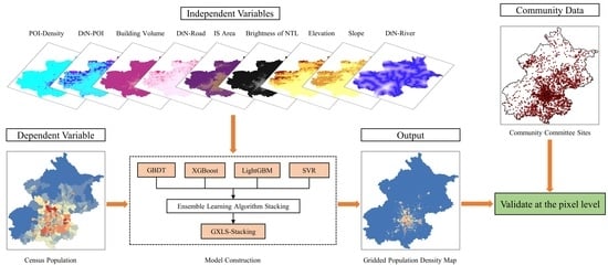
3.1. Overall Work Framework

Numerous factors influence the spatial distribution of a population. For a more comprehensive analysis of the spatial distribution of a population, we take into account not only the influence of natural environmental factors, but also the influence of the socioeconomic factors that better characterize the spatial distribution of the population. As mentioned earlier, we generated six categories of socioeconomic features, including POI-Density, DtN-POI, Building Volume, DtN-Road, IS Area and Brightness of NTL, and three categories of natural environmental features, including Elevation, DtN-River and Slope. These features collectively affect the spatial distribution of the population. As these factors interact with each other and are difficult to separate, their relationships with population density become complex and nonlinear [39].

Machine learning models can solve complex nonlinear problems, among which random forest models are widely used in the study of population spatialization and have shown high accuracy [35]. However, due to the complexity of the population spatialization problem, predicting population density becomes a very difficult regression problem. Although the random forest model can perform the regression task well, a good regression model does not reach all-round superiority over others. In addition, the accuracy of the random forest model still leaves much room for improvement due to the limited understanding of the variable features by the individual model. In this situation, a reasonable approach is to keep all the results of the excellent regression models and then create a final model by integrating them [43]. Ensemble learning algorithm stacking enables the integrated model to achieve better performance through the integration of heterogeneous models [44]. This paper aims to integrate the above multiple features, and constructs a novel population spatialization model GXLS-Stacking by integrating GBDT, XGBoost, LightGBM and SVR through stacking to generate a 100 m spatial resolution gridded population density map for Beijing in 2020. The detailed algorithms and model architecture are described in the following sections.

First, during the training phase, a total of 61 raster layers with 100 m spatial resolutions for the nine features mentioned above (22 POI-Density raster layers, 22 DtN-POI raster layers, 11 DtN-Road raster layers, 1 Building Volume raster layer, 1 IS Area raster layer, 1 Brightness of NTL raster layer, 1 Elevation raster layer, 1 DtN-River raster layer, 1 Slope raster layer) were used as the independent variables, and the census population was used as the dependent variable to fit the GXLS-Stacking, GBDT, XGBoost, LightGBM, SVR, and RF models. As the performance of these models may be biased by the division of the training and testing sets, we used the ten-fold cross-validation technique to evaluate the models and tune the hyperparameters of each model [75]. Then, during the prediction phase, all 61 raster layers were imported into the best trained models to predict the distributed weight and disaggregate the census population to generate the final dasymetric population density maps for Beijing in 2020. Finally, we used the highest spatial resolution validation data (i.e., community household registration data) to verify the accuracy at the pixel level to demonstrate that our integrated model GXLS-Stacking is not only better than the four individual models but also better than the random forest model. We also compared the highest spatial resolution and the best accuracy of the WorldPop mainland China dataset to demonstrate the superiority not only of the GXLS-Stacking model but also of our feature engineering. The flowchart of the proposed framework is shown in Figure 3.

3.2. Population Spatialization Model GXLS-Stacking

3.2.1. Stacked Generalization

Stacking is a hierarchical ensemble learning algorithm. It introduces the concept of meta-learning, i.e., integrates multiple base learners through a meta-learner, the base learners use the entire training set for training, while the meta-learner uses the results of the base learners as features to model. Besides, stacking represents an asymptotically optimal learning system, and aims to minimize the errors of generalization by reducing the bias of its generalizers [41]. When using stacking for model fusion, the improvement in prediction results is evident. This occurs because models with different generalization principles tend to yield different results. Diversity can be included in the modeling process by introducing models that follow different learning strategies. The diversity in stacking is achieved by using heterogeneous models on the same training sets [44]. Therefore, stacking’s advantages can be summarized as follows. Compared to individual models, it has better generalization ability, better modeling nonlinear patterns, and better identification of regressor variable importance [43].

There is a complex nonlinear relationship between the various population spatial distribution influencing factors and the population density. It is difficult for an individual model to completely fit this nonlinear relationship. Therefore, integrating individual models with excellent performance and giving full play to the characteristics of all the models can not only make the integrated model more diverse but also helps it better understand the variable features, improve the generalization ability, and make the final population spatialization result more accurate. Based on the above theories, we integrated the GBDT, XGBoost, LightGBM and SVR models, which not only performed well in ten-fold cross-validation but also have different learning strategies through ensemble learning algorithm stacking, and constructed a novel population spatialization model GXLS-Stacking to predict the spatial distribution of population with high precision. Where “G” stands for GBDT, “X” stands for XGBoost, “L” stands for LightGBM, and “S” stands for SVR.

3.2.2. Base Model and Meta-Model

Since stacking is a hierarchical ensemble learning algorithm, it expresses the concepts of a base model and meta-model. The selection of the base model and meta-model is very important because it is directly related to the accuracy of the final population spatialization results. After a repeated number of extensive experiments, GBDT, XGBoost and LightGBM were selected as the base models of the first layer because the base models must be accurate and different, i.e., have high accuracy during the training phase and follow different learning strategies so that diversity can be included in the modeling process, while the relatively simple but highly accurate SVR model was chosen as the meta-model of the second layer to avoid overfitting [43]. The basic principles and learning strategies of the base models and meta-model are described below. The detailed integration process is described in the following sections.

The gradient boosting decision tree (GBDT) is an ensemble learning model based on classification and regression trees (CART) and is trained by a gradient boosting algorithm. As an iterative decision tree algorithm, GBDT is composed of multiple trees, and the conclusion of all the trees is accumulated as the final answer. The gradient boosting algorithm builds a new model in the direction of the negative gradient of the previous model’s loss function, which is quite different from the traditional boosting algorithm with weighting samples. Therefore, the construction of each tree in GBDT makes the residuals decrease toward the negative gradient direction, and the model residuals decrease continuously in successive iterations [76].

Extreme gradient boosting (XGBoost) is a classic tree-based model. XGBoost has attracted increased attention and has been widely used in many recent data mining competitions due to its excellent performance. First, it penalizes complex models by adding regular terms to the objective function, effectively avoiding overfitting. Second, it uses the second-order approximation of the loss function while training, which speeds up the descent of the loss function and makes iterations faster. Third, it constructs an approximate algorithm for split finding and a sparsity-aware split-finding algorithm for automatically handling missing values, which can greatly improve the computational efficiency [77].

The light gradient boosting machine (LightGBM) is an adaptive gradient boosting model. To improve the computing power and prediction accuracy, the LightGBM first uses the histogram algorithm for split finding and the mutually exclusive feature bundling algorithm for feature dimension reduction, which can greatly reduce the time complexity. Second, the Leaf-wise algorithm is used to find the leaf with the greatest splitting gain from all the current leaves and then split it. At the same time, LightGBM adds a maximum depth limit on top of Leaf-wise to ensure high efficiency while preventing overfitting [78].

Initially, support vector machines (SVM) aimed to learn a separate function that divides training instances into distinct groups according to their class labels. Now, SVM has been extended for general estimation and prediction problems, namely, support vector regression (SVR). SVR is a nonlinear kernel-based regression model that attempts to find the best regression hyperplane with the smallest structural risk. SVR finds a function that approximates the training instances well by minimizing the prediction error. When minimizing the error, the risk of overfitting is reduced by simultaneously trying to maximize the flatness of the function [79].

3.2.3. Overall Model Architecture

The GXLS-Stacking model architecture of this paper is shown in Figure 4; it uses a two-layer ensemble learning algorithm stacking. GBDT, XGBoost and LightGBM are the base models of the first layer, and the SVR model is the meta-model of the second layer. The training and testing process of the GXLS-Stacking model is as follows. First, a five-fold cross-validation on the training set is applied for each base model in the first layer, and the predictions on the test set are calculated for each cross-validation. In the second layer, the five predictions of each base model on the training set are stitched together separately, which are the predictions of the original entire training set, and the predictions of the three base models of GBDT, XGBoost and LightGBM after stitching are combined as the input values of the second layer. The true values of the training set are used as the target values to train the meta-model SVR. Then, the mean values of the predictions of the three base models on the test set are combined and input to the SVR model to finally obtain the test result of the GXLS-Stacking model on the test set.

3.3. Random Forest Model for Comparison

Random forest (RF) is a tree-based bagging model. It randomly extracts m sub-samples and k sub-features from the original dataset, forming multiple sets of sub-data for training multiple regression trees. Then, it applies the averaging method to combine the regression results of each regression tree and generate the final regression results. The random forest model introduces a random attribute selection process while training, which makes the diversity of the base regression trees come not only from the sample disturbance but also from the attribute disturbance. Therefore, the generalization performance of random forest can be further improved by increasing the difference degree between the base regression trees [80]. Due to the excellent performance of the random forest model, it has been widely used in the study of population spatialization and has produced highly accurate results. Therefore, to evaluate the performance of the GXLS-Stacking model, we compared it with the random forest model.

3.4. Evaluation Strategy and Performance Metrics

An accuracy assessment is the validation of a model’s precision and is an important step for constructing a model. An ideal measure to validate the population spatialization results would be to use census counts with a finer resolution but this is very difficult due to the lack of census data or the corresponding boundary data [13]. However, we obtained community household registration data from the Information Center of the Ministry of Civil Affairs, which can be considered the highest resolution validation data [38]. To fully assess the accuracy of the best performing model, we used these data for validation at the pixel level.

Three performance metrics widely used for population spatialization, the determination coefficient (R²), mean absolute error (MAE) and root mean square error (RMSE), were adopted in this study. Given the research context of this paper, the units of MAE and RMSE are persons/hectare. The equations used to calculate these metrics are as follows:

$$R^2=\frac{{{\displaystyle \sum }}_{i=1}^n{\left({\widehat{y}}_i-\overline{y}\right)}^2}{{{\displaystyle \sum }}_{i=1}^n{\left(y_i-\overline{y}\right)}^2}$$

(2)

$$MAE=\frac{1}{n}{\displaystyle \sum }_{i=1}^n\left|y_i-{\widehat{y}}_i\right|$$

(3)

$$RMSE=\sqrt{\frac{1}{n}{\displaystyle \sum }_{i=1}^n{\left(y_i-{\widehat{y}}_i\right)}^2}$$

(4)

where $y_i$ is the true value, ${\widehat{y}}_i$ is the predicted value, $\overline{y}$ is the average of true values and $n$ is the total number of samples.

4. Results

4.1. Optimal Model Construction

We trained the models by using normalized training data and adjusting the hyperparameters of the models to obtain the optimal models. First, a total of 61 raster layers with 100 m spatial resolutions for the nine features mentioned above (22 POI-Density raster layers, 22 DtN-POI raster layers, 11 DtN-Road raster layers, 1 Building Volume raster layer, 1 IS Area raster layer, 1 Brightness of NTL raster layer, 1 Elevation raster layer, 1 DtN-River raster layer, 1 Slope raster layer) were normalized using Equation (5) and averaged at the township-level administrative unit. Then, the average population density was calculated by dividing the census population by the area (hectare) of the corresponding township-level administrative unit. Finally, the raster layers and the corresponding natural logarithms of the average population density were connected to fit the GXLS-Stacking, GBDT, XGBoost, LightGBM, SVR and RF models.

$$R{L}_i{}^{\prime }=\frac{R{L}_i-R{L}_{min}}{R{L}_{max}-R{L}_{min}}$$

(5)

where $R{L}_i{}^{\prime }$ is the normalized value of the $i$-th pixel of the raster layer, $R{L}_i$ denotes the original value of the $i$-th pixel of the raster layer, $R{L}_{max}$ represents the maximum value of the raster layer, and $R{L}_{min}$ is the minimum value of the raster layer.

The training, testing and validation processes of the above models were implemented using the xgboost, lightgbm and scikit-learn packages in Python (https://xgboost.readthedocs.io/en/stable/, https://lightgbm.readthedocs.io/en/latest/, https://scikit-learn.org/stable/ (accessed on 1 March 2022)). In order to improve the performance of the models, this study used the grid search method combined with ten-fold cross-validation technique to train the models and select the best hyperparameters to ensure that the optimal models were obtained [81]. The hyperparameters of the optimal models and their performance metrics in the ten-fold cross-validation are shown in

Table 3. The hyperparameters of the optimal models and their performance metrics in the ten-fold cross-validation.

Model Name	Ten-Fold Cross-Validation Performance Metrics			Global Optimal Hyperparameters
	R2	MAE	RMSE
GXLS-Stacking	0.9687	0.2564	0.3639	GBDT	max_depth: 3 max_features: 8 learning_rate: 0.2 n_estimators: 183 min_samples_split: 32
				XGBoost	n_estimators: 11 reg_lambda: 0.89 learning_rate: 0.38 gamma: 0.06 reg_alpha: 0.04 subsample: 0.7 max_depth: 8
				LightGBM	max_depth: 5 subsample: 0.1 reg_lambda: 0.19 learning_rate: 0.1 n_estimators: 132 feature_fraction: 0.7 min_child_samples: 39 min_child_weight: 0.001 num_leaves: 6 reg_alpha: 0.39
				SVR	gamma: 0.11C: 8 kernel: rbf
GBDT	0.9651	0.2722	0.3874	min_samples_split: 32 max_depth: 3 n_estimators: 76 max_features: 19 learning_rate: 0.26
XGBoost	0.9635	0.2824	0.3972	gamma: 0.195 reg_alpha: 0 subsample: 1 max_depth: 5 reg_lambda: 1 n_estimators: 17 learning_rate: 0.3 min_child_weight: 1
LightGBM	0.9658	0.2704	0.3836	feature_fraction: 0.42 min_child_samples: 8 min_child_weight: 0.001 max_bin: 170 max_depth: 4 num_leaves: 6 reg_alpha: 0.04 subsample: 0.01 reg_lambda: 0.31 learning_rate: 0.1 n_estimators: 138
SVR	0.9563	0.3049	0.4371	gamma: 0.24 C: 5 kernel: rbf
RF	0.9643	0.2729	0.3920	max_depth: 11 n_estimators: 30 max_features: 29 min_samples_split: 2

.

The GXLS-Stacking model achieved excellent results for performance metrics (i.e., R², MAE, RMSE) in the ten-fold cross-validation, where the R² was 0.9687, MAE was 0.2564 persons/hectare and RMSE was 0.3639 persons/hectare. In comparison with the four individual models GBDT, XGBoost, LightGBM, SVR and RF model, the three performance metrics of the GXLS-Stacking model were the highest. It is worth noting that all models achieved good results for the performance metrics in the ten-fold cross-validation, which indicates an overall agreement between the population density predicted by all models and the target population density. The results show that the overall performance of the GXLS-Stacking model was the best among the six models, so the GXLS-Stacking model is more likely to achieve the best accuracy in subsequent pixel level verification using community household registration data. Therefore, in the remainder of this study, we focused on using the GXLS-Stacking model that has been trained and achieved the best performance.

4.2. Dasymetric Population Mapping

Dasymetric mapping, also called dasymetric modeling, is a kind of areal interpolation that aims to disaggregate coarse resolution variables (e.g., population) to a finer resolution based on auxiliary data [7,45,82]. Dasymetric population mapping has a long history and has gained popularity due to the rapid development of the geographic information system and satellite remote sensing. Its key idea is to produce a gridded weight layer, and assuming the same spatial distribution of the population and the weight layer within the spatial unit [18,45,83]. Therefore, generating the population distribution weight layer is the penultimate step of the whole population spatialization process, and then disaggregating the census population based on this weight layer to finally obtain the gridded population density map.

Above, we obtained six optimal models (i.e., GXLS-Stacking, GBDT, XGBoost, LightGBM, SVR, RF) by the grid search method and ten-fold cross-validation technique. Then, the 61 raster layers mentioned above were positioned to the optimal models to predict the population distribution weight for each one hectare (i.e., 0.01 km²) gridded area (see Figure 5) and generated six 100 m spatial resolution distribution weight layers. Next, the distribution weight layers were used to disaggregate the census population at the township level administrative unit (see Figure 1) into pixels. Finally, six dasymetric population density maps (see Figure 6) for Beijing were produced using Equation (6) as follows:

$$PO{P}_{grid}=\frac{PO{P}_{township}\times W_{gird}}{W_{township}}$$

(6)

where $W_{gird}$ is the population distribution weight for a 1-hectare gridded area, $W_{township}$ denotes the summed population distribution weight of a township-level administrative unit that contains the gridded area, $PO{P}_{township}$ represents the township-level administrative unit census population, and $PO{P}_{grid}$ is the predicted population for the gridded area.

4.3. Accuracy Assessment of the Optimal Models

The assessment of gridded population density maps generated by the optimal models after the dasymetric population mapping has been a very difficult problem due to the lack of higher-resolution validation data [2,13,84,85]. Most of the current studies only conduct an overall assessment at the township level administrative unit, i.e., comparing the predicted total population with the corresponding township-level administrative unit census population [31,36,37,48,62]. However, the area of the township-level administrative unit is so large that even if the two values are consistent, they cannot represent the accurate spatial distribution of the population. Community data are considered to be the smallest scale and highest resolution validation data, and few scholars use it in their studies due to their difficult access [32,36,38]. Fortunately, the Information Center of the Ministry of Civil Affairs provided us with 3485 community household registration data in Beijing, and the detailed data processing flow is described above. Then, we evaluated the accuracy of the gridded population density maps generated by the optimal models on 3485 pixels. The detailed evaluation results are shown in Figure 7.

The GXLS-Stacking model achieved excellent results in the performance metrics (i.e., R², MAE, RMSE) in the pixel-level validation. Where the R² was 0.8004, MAE was 34.67 persons/hectare and RMSE was 54.92 persons/hectare. Compared to the other five models, the GXLS-Stacking model had the highest three performance metrics, which also represents its best overall performance. Compared with the four individual models GBDT, XGBoost, LightGBM and SVR, the overall performance of the integrated model GXLS-Stacking is far superior to these four individual models. This result shows that the GXLS-Stacking model can fully exert the characteristics of all the individual models and include diversity in the modeling process. In addition, the GXLS-Stacking model can better understand the complex nonlinear relationship between the various influencing factors of population spatial distribution and the population density, and can better identify the importance of the regression variables. Through the verification at the pixel level, it can be shown that the GXLS-Stacking model has a stronger generalization ability. The overall performance of the random forest model ranked second, where the R² was 0.7769, MAE was 36.47 persons/hectare and RMSE was 58.07 persons/hectare. This is why random forest models have been widely used in the study of population spatialization and have shown considerable accuracy. As shown in Figure 7, the scatter of the GXLS-Stacking model fits closely to the 1:1 line, and the other five models are discrete in some places. On the other hand, the weight layers can also be used as a criterion to evaluate the model performance. We found that the GXLS-Stacking model is still the best among the six models by computing the sum of all the pixel values in the weight layers and comparing it with the census population. The sum of all pixel values in the weight layer generated by the GXLS-Stacking model was the closest to the census population, with a difference of 60,797 persons. The results are shown in

Table 4. The sum of all pixel values in the weight layers compared with census population.

Model Name	Sum of All Pixels Values in Weight Layer	Census Population	Difference
GXLS-Stacking	21,832,298	21,893,095	−60,797
GBDT	25,122,462		3,229,367
XGBoost	20,115,082		−1,778,013
LightGBM	22,480,540		587,445
SVR	26,696,073		4,802,978
RF	22,409,335		516,240

.

4.4. WorldPop Mainland China Dataset for Comparison

The WorldPop dataset was reported as the most accurate gridded population density dataset with the finest spatial resolution (i.e., 100 m) for China in the current literature [48,62,74,86]. Therefore, by making comparisons with the WorldPop dataset, we can prove the superiority of not only the GXLS-Stacking model but also our feature engineering. Since the total population of Beijing in 2020 estimated by the WorldPop dataset was 18,617,470, which deviates widely from the official census population of 21,893,095, for the sake of fairness, we take the WorldPop dataset as a weight layer, and use the census data to make corrections to obtain a corrected WorldPop dataset. The WorldPop dataset and corrected WorldPop dataset are shown in Figure 8, and the scatter plots evaluated by the three performance metrics are shown in Figure 9. Although it can be seen from the scatter plots that the corrected WorldPop dataset is closer to the 1:1 line than the WorldPop dataset, both have an unacceptable inaccuracy (the R² was 0.1386 and 0.0399, respectively).

The WorldPop dataset was produced by generating weight-layer based on the random forest model and disaggregating the census population using the dasymetric mapping method, which is consistent with the logic of this study. However, the R² of the gridded population density map generated by the random forest model in this study reached 0.7769, which is much higher than the result of the WorldPop dataset. The reason for this phenomenon, we believe, is that our feature engineering performs far better than WorldPop. Through the WorldPop dataset production process [87], we found that the data they use are almost all publicly available and free, and most of them are land cover/land use data, net primary productivity (NPP), annual average temperature data and annual average precipitation data. However, these data are not directly indicative of human presence. They also have limited capabilities in extracting the demographic and socioeconomic features related to human activities, particularly in complex urban environments [48,49,50,51]. We use socioeconomic data that better characterize the spatial distribution of the population, such as the POI data, building outline data with height, artificial impervious surface data and road network data [7,48,58,73]. Among them, the POI data, building outline data and road network data are commercial data that have undergone a strict quality review. Compared with WorldPop, which uses similar data from World Food Programme (WFP) and OpenStreetMap (OSM) such as POI, road network, river network, etc. Our data are more comprehensive and of better quality and are more adaptable to complex population spatialization problems. Therefore, the data and features determine an upper-bound on the accuracy of the population spatialization results, and better models can approximate this bound more closely (e.g., the GXLS-Stacking model).

5. Discussion

5.1. Socioeconomic Features versus Natural Environmental Features

Our GXLS-Stacking model achieved the best accuracy in pixel-level validation. Therefore, to better understand why the model can achieve excellent results, we need to perform a feature importance evaluation of the model. As mentioned earlier, we have a total of six categories of socioeconomic features and three categories of natural environment features. To evaluate the importance of the different features in predicting the spatial distribution of the population, we selected the permutation feature importance technique, which is defined as the decrease in prediction accuracy when a predictor variable is randomly permuted [80]. Compared with the widely used measure of feature importance based on the decrease in the impurity of the tree-based models, permutation-based feature importance is less likely to be biased toward variables with many categories [75,88]. The results of the permutation-based feature importance assessment for the GXLS-Stacking model are shown in Figure 10.

The results showed that six categories of socioeconomic features ranked in the top six of feature importance, and three categories of natural environmental features ranked in the bottom three. The sum of the importance of socioeconomic features was as high as 99.54%, and the sum of importance of natural environmental features was only 0.46%. Among them, the sum of the importance of the POI-Density, DtN-POI and Building Volume features reached 94.52%, which fully indicated that the GXLS-Stacking model takes into account more of the influence of these features in the modeling process. In modern society, human existence inevitably generates demand for different kinds of services, driving the emergence of different service entities (e.g., hotels, schools, hospitals, restaurants, shopping malls). The larger the population, the greater the demand for such service entities, so areas with more POI or closer to POI have a larger population than their counterparts [31,36,37,48,56,89]. People live in buildings most of the day; compared with the 2-dimensional building area, the 3-dimensional building volume information can better reflect the capacity of the building to accommodate people. Therefore, areas with larger building volumes tend to have more people, and many studies have also shown that building volume has a strong positive correlation with population density [2,36,57,61,73,90]. This is why the sum of the importance of these three features is so high. Similarly, humans are more distributed near roads and in building areas from impervious surfaces, so these two features are of some importance [7,59,91,92].

DMSP-OLS nighttime light data have been widely used to assess the spatial distribution of populations and have shown a strong correlation [7,46,63,64,65]. We used NPP-VIIRS nighttime light data with better quality and higher spatial resolution than DMSP-OLS [68], but, surprisingly, the importance of the brightness of NTL feature is only 0.47%. The basic logic of using the brightness of NTL to distribute populations is that areas with bright lights at night usually have a large population [64]. However, the blooming effect is inherent to NTL and indicates that the peri-urban areas are illuminated by city lights [93]. Therefore, NTL within a small land area inside a city can brighten a large surrounding area [94]. In addition, although NPP-VIIRS does not have the saturation effect of DMSP-OLS and has a higher spatial resolution (i.e., 500 m), it is still not sufficient to reflect the population density in a small geographic area within the city due to the abovementioned problems.

In general, socioeconomic features can better characterize the spatial distribution of populations than the natural environmental features [36,37,38,87]. Indeed, the natural environmental features play a role in determining the spatial distribution of the population, as shown in Figure 6. Most of the population is located in the flat area of southeastern Beijing, while the surrounding high-altitude areas are rarely inhabited by humans. However, when both socioeconomic and natural environmental features are present, the socioeconomic features are more reflective of human activity and existence.

Compared with geographic weighted models that mainly rely on linear regression in previous population spatialization studies [13], machine learning models can explain the complex nonlinear relationship between the various population spatial distribution-influencing factors and the population density. The partial dependence plots (Figure 11) show the nonlinear relationship between the input variables and the population density in the GXLS-Stacking model. Most human settlements are distributed in the southeastern low elevation and flat areas of Beijing, and the population density decreases with increasing elevation and slope. From the perspective of socioeconomic features, the population density increases with an increasing POI density, building volume, impervious surface area, and brightness of NTL and decreases with an increasing distance to the nearest POI. The fitted curves show that the overall population density decreases with an increasing distance to the nearest road, but interestingly, the population density increases and then decreases around the x-axis of 0. We believe this phenomenon is because a small distance from the road, such as the presence of buildings, leads to an increase in population density and thus more people than on the road; when the population density reaches a maximum, the decrease in population density is caused by the reduction in human activity farther from the road. Similarly, the overall population density increases with an increasing distance to the nearest river but there is a peak in population density, which also indicates that certain distances from the river are more livable.

5.2. Cons and Pros of the GXLS-Stacking Model and Future Improvement

The GXLS-Stacking model is an ensemble-learning-based model, developed by integrating four individual models, GBDT, XGBoost, LightGBM and SVR, and based on the relationship between relevant geographic variables and the population density [41,76,77,78,79]. The GXLS-Stacking model can fully exert the characteristics of the four individual models; it can better understand the complex nonlinear relationships between various influencing factors of population spatial distribution and population density; it can better identify the importance of the regression variables; and it has stronger generalization abilities. Therefore, the GXLS-Stacking model achieves the best comprehensive performance in the validation at the pixel level. In addition, the GXLS-Stacking model also performs better than the random forest model, which is the most widely used in population spatialization studies and exhibits very high accuracy [2,36,37,38,48,80,87].

Currently, the GXLS-Stacking model has some limitations, as it integrates four individual models through ensemble learning algorithm stacking, so there is a problem of computational cost in the prediction process, but this problem is acceptable because of its high accuracy [43,95,96]. In addition, machine learning based models are data-driven models [97], so the GXLS-Stacking model will have higher requirements on the comprehensiveness and quality of data. For example, we consider subway line data and building outline data with height in the modeling process because it is helpful to disaggregate the census data, but in some small- and medium-sized cities, there are no subways and no building outline data with height, which will challenge the applicability of the GXLS-Stacking model. However, we believe that the GXLS-Stacking model will perform very well in metropolises with comprehensive and high-quality data, whether in China or in other countries. From a method perspective, our GXLS-Stacking model can better understand the complex nonlinear relationships between the various influencing factors of population spatial distribution and the population density, so even with some missing features, we believe it is more likely to perform well than the other five models. Therefore, for small- and medium-sized cities, our modeling process still provides an effective reference for their population spatialization methods.

As mentioned above, the data and features determine an upper bound on the accuracy of the population spatialization results, and better models can approximate this bound more closely. The NPP-VIIRS nighttime light data used in our modeling process are insufficient to portray a fine spatial distribution of the population due to its low spatial resolution. Compared to NPP-VIIRS, the Luojia 1-01 nighttime light data have a higher spatial resolution (i.e., 130 m), can detect a higher dynamic range, and better reflect the subtle human activities inside the city. Nevertheless, some issues remain when Luojia 1-01 data are used. First, these data contain slight geo-referencing errors, which cause mismatches with other remote sensing data. Second, some Luojia 1-01 images are affected by clouds and moonlight, so they cannot be used directly. Third, current Luojia 1-01 imagery is comprised of single images, which is an obstacle to applications over large areas [98]. Most importantly, Luojia 1-01 does not currently have data for Beijing in 2020 to match the timing of the other data in this study. In addition, the building outline data from Baidu Map obtained in our research are not classified according to their functions, which may also lead to a reduction of the population spatialization accuracy; because with the same building volume but different building functions, the number of people who can be accommodated is often different [32,99]. Although our POI data, road network data, and building outline data with height are all commercial data with strict quality validations, there is also the problem of missing data in suburban or rural areas, which can cause the GXLS-Stacking model to underestimate the population in these areas. According to related studies, the use of cropland data may be useful to improve the precision of population spatialization in rural areas, which may improve the underestimation of population density in these areas by the GXLS-Stacking model [100,101,102]. We believe that after solving these problems, the performance of the GXLS-Stacking model in the process of population spatialization will be further enhanced.

6. Conclusions

In this study, we integrated four individual models: GBDT, XGBoost, LightGBM, and SVR through ensemble learning algorithm stacking to construct a novel population spatialization model GXLS-Stacking. In addition, socioeconomic data and natural environmental data were integrated into the modeling to generate a gridded population density map with a 100 m spatial resolution for Beijing in 2020. Ten-fold cross-validation results and validation at the pixel level using community household registration data demonstrated that the GXLS-Stacking model can accurately predict the spatial distribution of a population. The major findings of this study are as follows.

Based on the various features extracted from multisource datasets, six optimal models were trained and obtained. The overall cross-validation R², MAE, and RMSE values of the GXLS-Stacking model were 0.9687, 0.2564 persons/hectare and 0.3639 persons/hectare, respectively, which were not only better than the four individual models but also better than the most widely used random forest model in population spatialization research. The GXLS-Stacking model also has the best performance in pixel-level verification, where R², MAE, and RMSE were 0.8004, 34.67 persons/hectare and 54.92 persons/hectare, respectively. This shows that the GXLS-Stacking model, compared to the four individual models and RF model, can better understand the complex nonlinear relationships between the various influencing factors of the population spatial distribution and the population density; it can better identify the importance of the regression variables; and it has stronger generalization abilities. The comparison with the WorldPop dataset shows that the data and features determine an upper bound on the accuracy of the population spatialization results, and the GXLS-Stacking model can approximate this bound more closely compared to the other five models. The result of the feature importance evaluation for the GXLS-Stacking model shows that when both the socioeconomic features and natural environmental features are present, the socioeconomic features are more able to characterize the spatial distribution of the population and the intensity of human activities.

In summary, our results show that the GXLS-Stacking model can predict the spatial distribution of populations with high precision, which is important for understanding the spatial patterns of population density. Moreover, the GXLS-Stacking model has the ability to be generalized to metropolises with comprehensive and high-quality data, whether in China or in other countries. Furthermore, for small- and medium-sized cities, our modeling process can still provide an effective reference for their population spatialization methods. Future studies may consider better types of socioeconomic data to improve the performance of the GXLS-Stacking model.

References

1. Gao, P.; Wu, T.; Ge, Y.; Li, Z. Improving the accuracy of extant gridded population maps using multisource map fusion. GISci. Remote Sens. 2022, 59, 54–70. [Google Scholar] [CrossRef]
2. Li, K.; Chen, Y.; Li, Y. The Random Forest-Based Method of Fine-Resolution Population Spatialization by Using the International Space Station Nighttime Photography and Social Sensing Data. Remote Sens. 2018, 10, 1650. [Google Scholar] [CrossRef] [Green Version]
3. Daughton, C.G. Wastewater surveillance for population-wide COVID-19: The present and future. Sci. Total Environ. 2020, 736, 139631. [Google Scholar] [CrossRef] [PubMed]
4. Jia, J.S.; Lu, X.; Yuan, Y.; Xu, G.; Jia, J.; Christakis, N.A. Population flow drives spatio-temporal distribution of COVID-19 in China. Nature 2020, 582, 389–394. [Google Scholar] [CrossRef]
5. Han, Y.; Yang, L.; Jia, K.; Li, J.; Feng, S.; Chen, W.; Zhao, W.; Pereira, P. Spatial distribution characteristics of the COVID-19 pandemic in Beijing and its relationship with environmental factors. Sci. Total Environ. 2021, 761, 144257. [Google Scholar] [CrossRef] [PubMed]
6. Zhao, G.; Yang, M. Urban Population Distribution Mapping with Multisource Geospatial Data Based on Zonal Strategy. ISPRS Int. J. Geo-Inf. 2020, 9, 654. [Google Scholar] [CrossRef]
7. Li, X.; Zhou, W. Dasymetric mapping of urban population in China based on radiance corrected DMSP-OLS nighttime light and land cover data. Sci. Total Environ. 2018, 643, 1248–1256. [Google Scholar] [CrossRef]
8. Pérez-Morales, A.; Gil-Guirado, S.; Martínez-García, V. Dasymetry Dash Flood (DDF). A method for population mapping and flood exposure assessment in touristic cities. Appl. Geogr. 2022, 142, 102683. [Google Scholar] [CrossRef]
9. Tenerelli, P.; Gallego, J.F.; Ehrlich, D. Population density modelling in support of disaster risk assessment. Int. J. Disaster Risk Reduct. 2015, 13, 334–341. [Google Scholar] [CrossRef]
10. Weber, E.M.; Seaman, V.Y.; Stewart, R.N.; Bird, T.J.; Tatem, A.J.; McKee, J.J.; Bhaduri, B.L.; Moehl, J.J.; Reith, A.E. Census-independent population mapping in northern Nigeria. Remote Sens. Environ. 2018, 204, 786–798. [Google Scholar] [CrossRef]
11. Li, L.; Li, J.; Jiang, Z.; Zhao, L.; Zhao, P. Methods of Population Spatialization Based on the Classification Information of Buildings from China’s First National Geoinformation Survey in Urban Area: A Case Study of Wuchang District, Wuhan City, China. Sensors 2018, 18, 2558. [Google Scholar] [CrossRef] [Green Version]
12. Xiong, J.; Li, K.; Cheng, W.; Ye, C.; Zhang, H. A Method of Population Spatialization Considering Parametric Spatial Stationarity: Case Study of the Southwestern Area of China. ISPRS Int. J. Geo-Inf. 2019, 8, 495. [Google Scholar] [CrossRef] [Green Version]
13. Wang, L.; Wang, S.; Zhou, Y.; Liu, W.; Hou, Y.; Zhu, J.; Wang, F. Mapping population density in China between 1990 and 2010 using remote sensing. Remote Sens. Environ. 2018, 210, 269–281. [Google Scholar] [CrossRef]
14. Jia, P.; Qiu, Y.; Gaughan, A.E. A fine-scale spatial population distribution on the High-resolution Gridded Population Surface and application in Alachua County, Florida. Appl. Geogr. 2014, 50, 99–107. [Google Scholar] [CrossRef]
15. Cheng, L.; Wang, L.; Feng, R.; Yan, J. Remote Sensing and Social Sensing Data Fusion for Fine-Resolution Population Mapping with a Multimodel Neural Network. IEEE J. Sel. Top. Appl. Earth Obs. Remote Sens. 2021, 14, 5973–5987. [Google Scholar] [CrossRef]
16. Azar, D.; Engstrom, R.; Graesser, J.; Comenetz, J. Generation of fine-scale population layers using multi-resolution satellite imagery and geospatial data. Remote Sens. Environ. 2013, 130, 219–232. [Google Scholar] [CrossRef]
17. Lung, T.; Lübker, T.; Ngochoch, J.K.; Schaab, G. Human population distribution modelling at regional level using very high resolution satellite imagery. Appl. Geogr. 2013, 41, 36–45. [Google Scholar] [CrossRef]
18. Briggs, D.J.; Gulliver, J.; Fecht, D.; Vienneau, D.M. Dasymetric modelling of small-area population distribution using land cover and light emissions data. Remote Sens. Environ. 2007, 108, 451–466. [Google Scholar] [CrossRef]
19. Chen, R.; Yan, H.; Liu, F.; Du, W.; Yang, Y. Multiple Global Population Datasets: Differences and Spatial Distribution Characteristics. ISPRS Int. J. Geo-Inf. 2020, 9, 637. [Google Scholar] [CrossRef]
20. Mei, Y.; Gui, Z.; Wu, J.; Peng, D.; Li, R.; Wu, H.; Wei, Z. Population spatialization with pixel-level attribute grading by considering scale mismatch issue in regression modeling. Geo-Spat. Inf. Sci. 2022, 1–18. [Google Scholar] [CrossRef]
21. Xie, Z. A Framework for Interpolating the Population Surface at the Residential-Housing-Unit Level. GISci. Remote Sens. 2013, 43, 233–251. [Google Scholar] [CrossRef]
22. Langford, M. Obtaining population estimates in non-census reporting zones: An evaluation of the 3-class dasymetric method. Comput. Environ. Urban Syst. 2006, 30, 161–180. [Google Scholar] [CrossRef]
23. Goodchild, M.F.; Anselin, L.; Deichmann, U. A Framework for the Areal Interpolation of Socioeconomic Data. Environ. Plan. A Econ. Space 1993, 25, 383–397. [Google Scholar] [CrossRef]
24. Bhaduri, B.; Bright, E.; Urban, C.M.L. LandScan USA: A high-resolution geospatial and temporal modeling approach for population distribution and dynamics. GeoJournal 2007, 69, 103–117. [Google Scholar] [CrossRef]
25. Goodchild, M.F.; Lam, N. Areal Interpolation—A Variant of the Traditional Spatial Problem. Geo-Processing 1980, 1, 297–312. [Google Scholar]
26. Holt, J.B.; Lo, C.P.; Hodler, T.W. Dasymetric Estimation of Population Density and Areal Interpolation of Census Data. Cartogr. Geogr. Inf. Sci. 2004, 31, 103–121. [Google Scholar] [CrossRef]
27. Harvey, J.T. Population estimation models based on individual TM pixels. Photogramm. Eng. Remote Sens. 2002, 68, 1181–1192. [Google Scholar]
28. Lwin, K.K.; Sugiura, K.; Zettsu, K. Space–time multiple regression model for grid-based population estimation in urban areas. Int. J. Geogr. Inf. Sci. 2016, 30, 1579–1593. [Google Scholar] [CrossRef]
29. Xu, Y.; Song, Y.; Cai, J.; Zhu, H. Population mapping in China with Tencent social user and remote sensing data. Appl. Geogr. 2021, 130, 102450. [Google Scholar] [CrossRef]
30. Douglass, R.W.; Meyer, D.A.; Ram, M.; Rideout, D.; Song, D. High resolution population estimates from telecommunications data. EPJ Data Sci. 2015, 4, 4. [Google Scholar] [CrossRef] [Green Version]
31. Yang, X.; Ye, T.; Zhao, N.; Chen, Q.; Yue, W.; Qi, J.; Zeng, B.; Jia, P. Population Mapping with Multisensor Remote Sensing Images and Point-Of-Interest Data. Remote Sens. 2019, 11, 574. [Google Scholar] [CrossRef] [Green Version]
32. Yao, Y.; Liu, X.; Li, X.; Zhang, J.; Liang, Z.; Mai, K.; Zhang, Y. Mapping fine-scale population distributions at the building level by integrating multisource geospatial big data. Int. J. Geogr. Inf. Sci. 2017, 31, 1220–1244. [Google Scholar] [CrossRef]
33. Zeng, C.; Zhou, Y.; Wang, S.; Yan, F.; Zhao, Q. Population spatialization in China based on night-time imagery and land use data. Int. J. Remote Sens. 2011, 32, 9599–9620. [Google Scholar] [CrossRef]
34. Wu, T.; Luo, J.; Dong, W.; Gao, L.; Hu, X.; Wu, Z.; Sun, Y.; Liu, J. Disaggregating County-Level Census Data for Population Mapping Using Residential Geo-Objects with Multisource Geo-Spatial Data. IEEE J. Sel. Top. Appl. Earth Obs. Remote Sens. 2020, 13, 1189–1205. [Google Scholar] [CrossRef]
35. He, M.; Xu, Y.; Li, N. Population Spatialization in Beijing City Based on Machine Learning and Multisource Remote Sensing Data. Remote Sens. 2020, 12, 1910. [Google Scholar] [CrossRef]
36. Qiu, G.; Bao, Y.; Yang, X.; Wang, C.; Ye, T.; Stein, A.; Jia, P. Local Population Mapping Using a Random Forest Model Based on Remote and Social Sensing Data: A Case Study in Zhengzhou, China. Remote Sens. 2020, 12, 1618. [Google Scholar] [CrossRef]
37. Wang, Y.; Huang, C.; Zhao, M.; Hou, J.; Zhang, Y.; Gu, J. Mapping the Population Density in Mainland China Using NPP/VIIRS and Points-of-Interest Data Based on a Random Forests Model. Remote Sens. 2020, 12, 3645. [Google Scholar] [CrossRef]
38. Zhou, Y.; Ma, M.; Shi, K.; Peng, Z. Estimating and Interpreting Fine-Scale Gridded Population Using Random Forest Regression and Multisource Data. ISPRS Int. J. Geo-Inf. 2020, 9, 369. [Google Scholar] [CrossRef]
39. Zhao, S.; Liu, Y.; Zhang, R.; Fu, B. China’s population spatialization based on three machine learning models. J. Clean. Prod. 2020, 256, 120644. [Google Scholar] [CrossRef]
40. Czarnowski, I.; Jedrzejowicz, P. An approach to machine classification based on stacked generalization and instance selection. In Proceedings of the 2016 IEEE International Conference on Systems, Man, and Cybernetics (SMC), Budapest, Hungary, 9–12 October 2016; pp. 4836–4841. [Google Scholar]
41. Wolpert, D.H. Stacked generalization. Neural Netw. 1992, 5, 241–259. [Google Scholar] [CrossRef]
42. Rose, S. Mortality Risk Score Prediction in an Elderly Population Using Machine Learning. Am. J. Epidemiol. 2013, 177, 443–452. [Google Scholar] [CrossRef] [Green Version]
43. Ribeiro, M.H.D.M.; Dos Santos Coelho, L. Ensemble approach based on bagging, boosting and stacking for short-term prediction in agribusiness time series. Appl. Soft Comput. 2020, 86, 105837. [Google Scholar] [CrossRef]
44. Agarwal, S.; Chowdary, C.R. A-Stacking and A-Bagging: Adaptive versions of ensemble learning algorithms for spoof fingerprint detection. Expert Syst. Appl. 2020, 146, 113160. [Google Scholar] [CrossRef]
45. Jia, P.; Gaughan, A.E. Dasymetric modeling: A hybrid approach using land cover and tax parcel data for mapping population in Alachua County, Florida. Appl. Geogr. 2016, 66, 100–108. [Google Scholar] [CrossRef]
46. Yu, S.; Zhang, Z.; Liu, F. Monitoring Population Evolution in China Using Time-Series DMSP/OLS Nightlight Imagery. Remote Sens. 2018, 10, 194. [Google Scholar] [CrossRef] [Green Version]
47. Zandbergen, P.A.; Ignizio, D.A. Comparison of Dasymetric Mapping Techniques for Small-Area Population Estimates. Cartogr. Geogr. Inf. Sci. 2010, 37, 199–214. [Google Scholar] [CrossRef]
48. Ye, T.; Zhao, N.; Yang, X.; Ouyang, Z.; Liu, X.; Chen, Q.; Hu, K.; Yue, W.; Qi, J.; Li, Z.; et al. Improved population mapping for China using remotely sensed and points-of-interest data within a random forests model. Sci. Total Environ. 2019, 658, 936–946. [Google Scholar] [CrossRef] [PubMed]
49. Liu, X.; He, J.; Yao, Y.; Zhang, J.; Liang, H.; Wang, H.; Hong, Y. Classifying urban land use by integrating remote sensing and social media data. Int. J. Geogr. Inf. Sci. 2017, 31, 1675–1696. [Google Scholar] [CrossRef]
50. Lu, D.; Tian, H.; Zhou, G.; Ge, H. Regional mapping of human settlements in southeastern China with multisensor remotely sensed data. Remote Sens. Environ. 2008, 112, 3668–3679. [Google Scholar] [CrossRef]
51. Liu, Y.; Liu, X.; Gao, S.; Gong, L.; Kang, C.; Zhi, Y.; Chi, G.; Shi, L. Social Sensing: A New Approach to Understanding Our Socioeconomic Environments. Ann. Assoc. Am. Geogr. 2015, 105, 512–530. [Google Scholar] [CrossRef]
52. Yao, Y.; Li, X.; Liu, X.; Liu, P.; Liang, Z.; Zhang, J.; Mai, K. Sensing spatial distribution of urban land use by integrating points-of-interest and Google Word2Vec model. Int. J. Geogr. Inf. Sci. 2017, 31, 825–848. [Google Scholar] [CrossRef]
53. Bakillah, M.; Liang, S.; Mobasheri, A.; Jokar Arsanjani, J.; Zipf, A. Fine-resolution population mapping using OpenStreetMap points-of-interest. Int. J. Geogr. Inf. Sci. 2014, 28, 1940–1963. [Google Scholar] [CrossRef]
54. Cai, J.; Huang, B.; Song, Y. Using multi-source geospatial big data to identify the structure of polycentric cities. Remote Sens. Environ. 2017, 202, 210–221. [Google Scholar] [CrossRef]
55. Zhao, Y.; Li, Q.; Zhang, Y.; Du, X. Improving the Accuracy of Fine-Grained Population Mapping Using Population-Sensitive POIs. Remote Sens. 2019, 11, 2502. [Google Scholar] [CrossRef] [Green Version]
56. Jiang, S.; Alves, A.; Rodrigues, F.; Ferreira, J.; Pereira, F.C. Mining point-of-interest data from social networks for urban land use classification and disaggregation. Comput. Environ. Urban Syst. 2015, 53, 36–46. [Google Scholar] [CrossRef] [Green Version]
57. Esch, T.; Brzoska, E.; Dech, S.; Leutner, B.; Palacios-Lopez, D.; Metz-Marconcini, A.; Marconcini, M.; Roth, A.; Zeidler, J. World Settlement Footprint 3D—A first three-dimensional survey of the global building stock. Remote Sens. Environ. 2022, 270, 112877. [Google Scholar] [CrossRef]
58. Lin, Y.; Zhang, H.; Lin, H.; Gamba, P.E.; Liu, X. Incorporating synthetic aperture radar and optical images to investigate the annual dynamics of anthropogenic impervious surface at large scale. Remote Sens. Environ. 2020, 242, 111757. [Google Scholar] [CrossRef]
59. Wei, S.; Lin, Y.; Zhang, H.; Wan, L.; Lin, H.; Wu, Z. Estimating Chinese residential populations from analysis of impervious surfaces derived from satellite images. Int. J. Remote Sens. 2021, 42, 2303–2326. [Google Scholar] [CrossRef]
60. Zhou, Y.; Lin, C.; Wang, S.; Liu, W.; Tian, Y. Estimation of Building Density with the Integrated Use of GF-1 PMS and Radarsat-2 Data. Remote Sens. 2016, 8, 969. [Google Scholar] [CrossRef] [Green Version]
61. Frantz, D.; Schug, F.; Okujeni, A.; Navacchi, C.; Wagner, W.; Van der Linden, S.; Hostert, P. National-scale mapping of building height using Sentinel-1 and Sentinel-2 time series. Remote Sens. Environ. 2021, 252, 112128. [Google Scholar] [CrossRef] [PubMed]
62. Gaughan, A.E.; Stevens, F.R.; Huang, Z.; Nieves, J.J.; Sorichetta, A.; Lai, S.; Ye, X.; Linard, C.; Hornby, G.M.; Hay, S.I.; et al. Spatiotemporal patterns of population in mainland China, 1990 to 2010. Sci. Data 2016, 3, 160005. [Google Scholar] [CrossRef]
63. Elvidge, C.D.; Baugh, K.E.; Dietz, J.B.; Bland, T.; Sutton, P.C.; Kroehl, H.W. Radiance Calibration of DMSP-OLS Low-Light Imaging Data of Human Settlements. Remote Sens. Environ. 1999, 68, 77–88. [Google Scholar] [CrossRef]
64. Sutton, P.; Roberts, D.; Elvidge, C.; Baugh, K. Census from Heaven: An estimate of the global human population using night-time satellite imagery. Int. J. Remote Sens. 2010, 22, 3061–3076. [Google Scholar] [CrossRef]
65. Imhoff, M.L.; Lawrence, W.T.; Stutzer, D.C.; Elvidge, C.D. A technique for using composite DMSP/OLS “city lights” satellite data to map urban area. Remote Sens. Environ. 1997, 61, 361–370. [Google Scholar] [CrossRef]
66. Cao, X.; Hu, Y.; Zhu, X.; Shi, F.; Zhuo, L.; Chen, J. A simple self-adjusting model for correcting the blooming effects in DMSP-OLS nighttime light images. Remote Sens. Environ. 2019, 224, 401–411. [Google Scholar] [CrossRef]
67. Small, C.; Pozzi, F.; Elvidge, C. Spatial analysis of global urban extent from DMSP-OLS night lights. Remote Sens. Environ. 2005, 96, 277–291. [Google Scholar] [CrossRef]
68. Elvidge, C.D.; Zhizhin, M.; Ghosh, T.; Hsu, F.; Taneja, J. Annual Time Series of Global VIIRS Nighttime Lights Derived from Monthly Averages: 2012 to 2019. Remote Sens. 2021, 13, 922. [Google Scholar] [CrossRef]
69. Zhang, X.; Liu, L.; Zhao, T.; Gao, Y.; Chen, X.; Mi, J. GISD30: Global 30 m impervious-surface dynamic dataset from 1985 to 2020 using time-series Landsat imagery on the Google Earth Engine platform. Earth Syst. Sci. Data. 2022, 14, 1831–1856. [Google Scholar] [CrossRef]
70. Zhong, Y.; Su, Y.; Wu, S.; Zheng, Z.; Zhao, J.; Ma, A.; Zhu, Q.; Ye, R.; Li, X.; Pellikka, P.; et al. Open-source data-driven urban land-use mapping integrating point-line-polygon semantic objects: A case study of Chinese cities. Remote Sens. Environ. 2020, 247, 111838. [Google Scholar] [CrossRef]
71. Decuyper, M.; Chávez, R.O.; Lohbeck, M.; Lastra, J.A.; Tsendbazar, N.; Hackländer, J.; Herold, M.; Vågen, T. Continuous monitoring of forest change dynamics with satellite time series. Remote Sens. Environ. 2022, 269, 112829. [Google Scholar] [CrossRef]
72. Dehnad, K. Density Estimation for Statistics and Data Analysis. Technometrics 2012, 29, 495. [Google Scholar] [CrossRef]
73. Cao, Y.; Huang, X. A deep learning method for building height estimation using high-resolution multi-view imagery over urban areas: A case study of 42 Chinese cities. Remote Sens. Environ. 2021, 264, 112590. [Google Scholar] [CrossRef]
74. Bai, Z.; Wang, J.; Wang, M.; Gao, M.; Sun, J. Accuracy Assessment of Multi-Source Gridded Population Distribution Datasets in China. Sustainability 2018, 10, 1363. [Google Scholar] [CrossRef] [Green Version]
75. Zhang, Y.; Liang, S.; Zhu, Z.; Ma, H.; He, T. Soil moisture content retrieval from Landsat 8 data using ensemble learning. ISPRS J. Photogramm. 2022, 185, 32–47. [Google Scholar] [CrossRef]
76. Friedman, J.H. Greedy function approximation: A gradient boosting machine. Ann. Stat. 2001, 29, 1189–1232. [Google Scholar] [CrossRef]
77. Chen, T.; Guestrin, C. XGBoost: A Scalable Tree Boosting System; ACM: San Francisco, CA, USA, 2016; pp. 785–794. [Google Scholar]
78. Ke, G.; Meng, Q.; Finley, T.; Wang, T.; Chen, W.; Ma, W.; Ye, Q.; Liu, T. LightGBM: A Highly Efficient Gradient Boosting Decision Tree. In Proceedings of the Advances in Neural Information Processing Systems 30 (NIPS 2017), Long Beach, CA, USA, 4–9 December 2017; p. 30. [Google Scholar]
79. Drucker, H.; Burges, C.; Kaufman, L.; Smola, A.; Vapnik, V. Support vector regression machines. Adv. Neural Inf. Processing Syst. 1997, 9, 155–161. [Google Scholar]
80. Breiman, L. Random forests. Mach. Learn. 2001, 45, 5–32. [Google Scholar] [CrossRef] [Green Version]
81. Bergstra, J.; Bengio, Y. Random Search for Hyper-Parameter Optimization. J. Mach. Learn. Res. 2012, 13, 281–305. [Google Scholar]
82. Pavía, J.M.; Cantarino, I. Can Dasymetric Mapping Significantly Improve Population Data Reallocation in a Dense Urban Area? Geogr. Anal. 2017, 49, 155–174. [Google Scholar] [CrossRef]
83. Dmowska, A.; Stepinski, T.F. A high resolution population grid for the conterminous United States: The 2010 edition. Comput. Environ. Urban Syst. 2017, 61, 13–23. [Google Scholar] [CrossRef]
84. Zhuo, L.; Ichinose, T.; Zheng, J.; Chen, J.; Shi, P.J.; Li, X. Modelling the population density of China at the pixel level based on DMSP/OLS non-radiance-calibrated night-time light images. Int. J. Remote Sens. 2009, 30, 1003–1018. [Google Scholar] [CrossRef]
85. Yang, X.; Yue, W.; Gao, D. Spatial improvement of human population distribution based on multi-sensor remote-sensing data: An input for exposure assessment. Int. J. Remote Sens. 2013, 34, 5569–5583. [Google Scholar] [CrossRef]
86. Xu, Y.; Ho, H.C.; Knudby, A.; He, M. Comparative assessment of gridded population data sets for complex topography: A study of Southwest China. Popul. Environ. 2021, 42, 360–378. [Google Scholar] [CrossRef]
87. Stevens, F.R.; Gaughan, A.E.; Linard, C.; Tatem, A.J. Disaggregating Census Data for Population Mapping Using Random Forests with Remotely-Sensed and Ancillary Data. PLoS ONE 2015, 10, e107042. [Google Scholar] [CrossRef] [Green Version]
88. Strobl, C.; Boulesteix, A.; Zeileis, A.; Hothorn, T. Bias in random forest variable importance measures: Illustrations, sources and a solution. BMC Bioinform. 2007, 8, 25. [Google Scholar] [CrossRef] [Green Version]
89. Gao, S.; Janowicz, K.; Couclelis, H. Extracting urban functional regions from points of interest and human activities on location-based social networks. Trans. GIS 2017, 21, 446–467. [Google Scholar] [CrossRef]
90. Alahmadi, M.; Atkinson, P.; Martin, D. Estimating the spatial distribution of the population of Riyadh, Saudi Arabia using remotely sensed built land cover and height data. Comput. Environ. Urban Syst. 2013, 41, 167–176. [Google Scholar] [CrossRef]
91. Kuang, W.; Hou, Y.; Dou, Y.; Lu, D.; Yang, S. Mapping Global Urban Impervious Surface and Green Space Fractions Using Google Earth Engine. Remote Sens. 2021, 13, 4187. [Google Scholar] [CrossRef]
92. Kuang, W.; Zhang, S.; Li, X.; Lu, D. A 30 m resolution dataset of China’s urban impervious surface area and green space, 2000–2018. Earth Syst. Sci. Data 2021, 13, 63–82. [Google Scholar] [CrossRef]
93. Li, X.; Zhou, Y. Urban mapping using DMSP/OLS stable night-time light: A review. Int. J. Remote Sens. 2017, 38, 6030–6046. [Google Scholar] [CrossRef]
94. Esch, T.; Marconcini, M.; Marmanis, D.; Zeidler, J.; Elsayed, S.; Metz, A.; Müller, A.; Dech, S. Dimensioning urbanization—An advanced procedure for characterizing human settlement properties and patterns using spatial network analysis. Appl. Geogr. 2014, 55, 212–228. [Google Scholar] [CrossRef]
95. Ting, K.M.; Witten, I.H. Issues in Stacked Generalization. J. Artif. Intell. Res. 1999, 10, 271–289. [Google Scholar] [CrossRef] [Green Version]
96. Anifowose, F.; Labadin, J.; Abdulraheem, A. Improving the prediction of petroleum reservoir characterization with a stacked generalization ensemble model of support vector machines. Appl. Soft Comput. 2015, 26, 483–496. [Google Scholar] [CrossRef]
97. Ning, C.; You, F. Optimization under uncertainty in the era of big data and deep learning: When machine learning meets mathematical programming. Comput. Chem. Eng. 2019, 125, 434–448. [Google Scholar] [CrossRef] [Green Version]
98. Ou, J.; Liu, X.; Liu, P.; Liu, X. Evaluation of Luojia 1-01 nighttime light imagery for impervious surface detection: A comparison with NPP-VIIRS nighttime light data. Int. J. Appl. Earth Obs. 2019, 81, 1–12. [Google Scholar] [CrossRef]
99. Zhuo, L.; Shi, Q.; Zhang, C.; Li, Q.; Tao, H. Identifying Building Functions from the Spatiotemporal Population Density and the Interactions of People among Buildings. ISPRS Int. J. Geo-Inf. 2019, 8, 247. [Google Scholar] [CrossRef] [Green Version]
100. Kuang, W. 70 years of urban expansion across China: Trajectory, pattern, and national policies. Sci. Bull. 2020, 65, 1970–1974. [Google Scholar] [CrossRef]
101. Kuang, W.; Du, G.; Lu, D.; Dou, Y.; Li, X.; Zhang, S.; Chi, W.; Dong, J.; Chen, G.; Yin, Z.; et al. Global observation of urban expansion and land-cover dynamics using satellite big-data. Sci. Bull. 2021, 66, 297–300. [Google Scholar] [CrossRef]
102. Kuang, W.; Liu, J.; Tian, H.; Shi, H.; Dong, J.; Song, C.; Li, X.; Du, G.; Hou, Y.; Lu, D.; et al. Cropland redistribution to marginal lands undermines environmental sustainability. Natl. Sci. Rev. 2022, 9, nwab091. [Google Scholar] [CrossRef]
Figure 1. Geographical location and census situation of Beijing.
Remotesensing 14 03654 g001
Figure 2. Spatial distribution of Beijing community committee sites.
Remotesensing 14 03654 g002
Figure 3. Flowchart of the proposed framework.
Remotesensing 14 03654 g003
Figure 4. GXLS-Stacking model overall architecture.
Remotesensing 14 03654 g004
Figure 5. The 100 m spatial resolution distribution weight layers predicted by the optimal models.
Remotesensing 14 03654 g005
Figure 6. The 100 m spatial resolution dasymetric population density maps for Beijing in 2020 generated by the optimal models.
Remotesensing 14 03654 g006
Figure 7. Scatter plots of the predicted by optimal models and the community committee sites population density at the pixel level (Total of 3485 pixels). A ln-ln transformation was conducted for the population density. The black dash line indicate 1:1 line. pph: persons per hectare.
Remotesensing 14 03654 g007
Figure 8. (a) WorldPop mainland China dataset in 2020. (b) WorldPop mainland China dataset corrected by census data in 2020. WPCBCD: WorldPop corrected by census data.
Remotesensing 14 03654 g008
Figure 9. (a) Scatter plot of the predicted by WorldPop and the community committee sites population density at the pixel level (Total of 3485 pixels). (b) Scatter plot of the predicted by WPCBCD and the community committee sites population density at the pixel level (Total of 3485 pixels). A ln-ln transformation was conducted for the population density. The black dash line indicate 1:1 line. pph: persons per hectare. WPCBCD: WorldPop corrected by census data.
Remotesensing 14 03654 g009
Figure 10. Permutation-based feature importance results of the GXLS-Stacking model.
Remotesensing 14 03654 g010
Figure 11. Partial dependency plots for the variables in the GXLS-Stacking model predicting population density (ai). The black ticks at the bottom of the plots are the distribution density of the input variables. The solid blue line is the fitted curve.
Remotesensing 14 03654 g011