
Ground Penetrating Radar Measurements in Shallow Water Environments—A Case Study


Institute of Geosciences, Christian-Albrechts-University of Kiel, Otto-Hahn-Platz 1, 24118 Kiel, Germany
*
Author to whom correspondence should be addressed.
Remote Sens. 2022, 14(15), 3659; https://0-doi-org.brum.beds.ac.uk/10.3390/rs14153659
Submission received: 15 May 2022
/
Revised: 18 July 2022
/
Accepted: 23 July 2022
/
Published: 30 July 2022
(This article belongs to the Special Issue Advances in Ground-Penetrating Radar for Archaeology)
Abstract
:In this study, we investigate GPR measurements in freshwater of less than 5 m at four different locations to derive rules of thumb in terms of depth penetration, resolution, and material contrasts of the method for 200 and 400 MHz antennas under field conditions. The objective is to improve the attractiveness of the method for archaeological issues in water, as there are hardly any studies on this subject so far. The depth penetration of 2–4 m is negligibly influenced by the choice of the 200 or 400 MHz antenna. Organic material in the water column also does not affect the water depth but offers new fields of applications for mapping and volume estimation of biomass in lakes with GPR. The horizontal resolution in the cm range in the direction of the profile and in the dm range across the profile could not be improved by the narrow antenna radiation pattern of <30° at the 3 dB level. In the crossline direction, the use of an antenna array would be necessary here. Still, the narrow antenna pattern reduces side reflections. Most common archaeological material contrasts can be resolved with the method. The method shows reflection coefficients >0.1 for materials of <80% porosity to the water column and for materials of <25% porosity and of >45% porosity to water-saturated sand. Large reflection coefficients also show, for example, granite to sand and gyttja to wood. The water column has a considerable effect on the data quality of the 400 MHz antenna from a depth of 2 m due to the antenna ringing. Furthermore, multiples must be expected in a water column <0.5 m. The method can especially complement the common geophysical methods of seismics and geoelectrics to exclude material ambiguities. The major advantage is the simple setting of the land equipment in the water.
1. Introduction
Ground-penetrating radar has been successfully applied for archaeological prospection of objects on land since the 1970s [1,2,3]. Although interest in submerged anthropogenic constructions, such as ancient harbour facilities, has gained much archaeological interest, the method has been used only rarely for archaeological prospection in shallow water zones. The common geophysical approach in marine and lacustrine archaeological investigations is seismic/acoustic measurements, providing a spatial resolution in the cm range and a depth of penetration of more than 20 m [4,5,6]. In recent years, geoelectric investigations were also used for the detection of archaeological objects in shallow water [7,8,9]. Here, an average spatial resolution in the dm-to-m range is achieved. Still, there are some situations where the usability of the common seismic and geoelectric methods is limited, and the application of GPR measurements in water appears to be advantageous. These advantages are as follows:
(a) Seismic measurements may not be possible due to an extremely shallow water column [10,11], may be affected by multiples, or may be attenuated by a gassy subsurface [12]. In particular, ref. [11] as well as [13] suggested a joint application of the methods of GPR and seismics in shallow water.
(b) In the presence of organic material in the water column, the authors of [14,15] were able to investigate the underlying bathymetry more accurately with GPR than with seismic surveys.
(c) A variety of material contrasts from submerged archaeological structures can be better resolved with GPR than with seismics. An example is the reflection coefficient of oak wood to wet sand [16].
(d) Special equipment is necessary for marine seismics and geoelectrics [17,18], whereas standard GPR antennas can be used in the water without much additional time and financial effort. In contrast, for GPR, only an appropriately watertight box is required, in addition to a small boat [19,20].
The main factor limiting the regular application of GPR in water is the high attenuation of electromagnetic waves with increasing salinity of the water [21]. Thus, there are only few examples investigating marine archaeological targets with GPR. The author of [22] was able to detect the archaeological layer of the bronze-age settlement “Greifensee-Böschen”, Switzerland, on a prospection area of 11 × 18 m. Ref. [23] contribute to the landscape reconstruction around a submerged archaeological site, distinguishing between beach and glaciolacustrine clay deposits. In [20], submerged GPR equipment was developed for archaeological investigations of submerged stonewalls in 2 m depth below a 1 m saltwater column. Some other studies focus on the detection of sunken objects in freshwater and below the bottom, for example, logs [19], jet skis [10], and munition [24], usually using 200 MHz and 400 MHz GPR antennas for a centimetre- to decimetre-scale resolution. In other areas of application, several studies using offshore GPR measurements were carried out, for example, in the prospection of ice shields and geological issues. The first GPR measurements on ice took place in the 1960s [25] and were investigating arctic regions, for the determination of ice thicknesses [26]. Other offshore applications of GPR have been the detection of groundwater [27] and of thermal boundaries [28]. In ref. [29,30,31], investigations are presented on the morphology, stratigraphy, and bathymetry in coastal ponds. Further applications are presented by [32], focusing on riverbed scour, and by [33], monitoring stream discharge. To improve the depth penetration, ref. [34] used a 5 m submerged 400 MHz antenna to prospect riverbed scour in 8 m depth. There are different studies determining the sedimentary type, for example, from diffraction hyperbola velocities presented by [35], and from determining reflection coefficients based on the ratios of reflected signal strengths from sediments and a reference aluminium plate [13].
Within the context of geological and ice shield investigations, extensive research has been carried out on the physical impact of the water column on GPR measurements for antenna frequencies of 60–150 MHz and water depths of more than 5 m [14,36,37,38]. Within these studies, parameters such as the spatial resolution, depth of penetration, and antenna pattern, as well as specific effects such as frequency reduction and antenna impedance loading, are discussed. Effects that occur specifically in water, such as “ringing” (horizontal stripes in the water column as a consequence of the high dielectric contrast between air and water), are regularly described. A more detailed overview will be given in the following chapters.
In the rare archaeological case studies using limnic GPR, there is no rule of thumb for practical considerations with respect to, for example, penetration depth or resolution. Moreover, if there were such a rule, would it hold true for very different measurement locations with respect to water depth, water conductivity, and organic matter content in the water column? To answer these questions, we present four datasets using offshore GPR in different limnic environments and using two typical antenna frequencies (200 and 400 MHz). With the help of these datasets, we focus on the following three thematic issues:
- The depth of penetration of GPR measurements depends on numerous factors, such as subsurface material and antenna properties. Is it still possible to determine basic rules of thumb for field applications? How do organic materials, such as leaves in the water column, affect the depth of penetration?
- Up to which degree can archaeological constructions be spatially resolved within the possible depth range? Which aspects have to be considered regarding the resolution along and across profile directions?
- For which archaeological material contrasts is the GPR method particularly suitable compared to seismics and electrics? Which additional areas of application arise?
To answer the three questions, we compare the results of previous studies and of theoretical considerations with our data measured under field conditions. For the third aspect, we determine theoretical archaeological material contrasts from both common sub-bottom and archaeological construction materials and compare these to our field data.
2. Measurement Locations
To answer the three issues of penetration depth, spatial resolution, and material contrasts of water-based GPR measurements under field conditions, we surveyed GPR profiles with both 400 MHz and 200 MHz GSSI antennas and an SIR 4000 registration unit at four different locations. The measurement locations differ in terms of water depth, water conductivity, and subsurface materials, as well as movement and stratification of the water column.
The first chosen measurement location (“flooded gravel pit”) is situated near Wörth at Rhine, Rhineland-Palatinate, Germany (Figure 1). Here, the gravelly shoreline slopes steeply to the center of the lake (yellow line), and we find the largest water depths of >4 m at all locations. Figure 1 shows exemplary measurement profiles of the 200 MHz and 400 MHz antennas at slightly different locations in the “flooded gravel pit”. This feature is useful for answering the question of the penetration depth as a function of the antenna frequency and the attenuation coefficient due to the water column. The noticeably high noise content in the water column, especially for the 400 MHz antenna (blue frame), invites us to analyze the data quality in relation to the water depth and the antenna frequency.
The second location chosen for GPR measurements, “swimming pool” (Figure 2), is weather protected and can be used for repeated measurements under constant conditions (water temperature, water conductivity). The sloping ground (yellow dashed line) is tiled. The question of the penetration depth for different antenna frequencies can be also investigated here. In addition, it was possible to lower an aluminum pipe of 7 cm diameter (red circle) in a controlled setting. From this, as well as from steps leading into the pool (blue frame), it was possible to address the issue of the spatial resolution under field conditions here.
The third location, “river”, a section of the Altmühl River, Bavaria, Germany (Figure 3), is the only measurement location with flowing water. Its subsurface (yellow line) mostly consists of sand or sandbars (Figure 3b). At some spots, larger boulders appear in clusters (Figure 3a) or fish pass below the antenna. The resulting diffraction hyperbolas (red circles) are again well suited for analyzing the spatial resolution under field conditions. In addition, especially in very shallow water <30 cm, further measurement effects are visible in the form of multiples (Figure 3b, green dotted lines), which must be considered when planning GPR measurements in water.
The last measurement location (“pond”), near Graben, Bavaria, Germany (Figure 4), is the flooded remnant of a collapsed trench. Its moderately sloping subsoil (yellow line) consists of mud (i.e., silty sediments and gyttja) due to leaves and wood from the surrounding trees. According to [39], gyttja is a combination of organic and inorganic materials precipitated from a lake water column via biogeochemical processes. Larger branches or tree trunks also cause diffraction hyperbolas (red circles). These conditions are again suitable for investigating the questions of depth penetration and spatial resolution. The most striking feature, however, is that different amounts of organic material can be found in the water column at various parts of the pond. There are parts with no organic material in the water column (Figure 4b, blue frame), as well as parts where no boat engine could be used due to the organic material in the water column (Figure 4b, green frame). From the direct comparison of lake bottom amplitudes, we can determine how much organic material in the water column scatters the GPR measurements and thus reduces the measured amplitudes in the radargram.
In addition, the subsurface materials of sand, gravel, mud, and tiles of all four measurement locations were used to investigate the issue of expected material contrasts. The most important environmental and measurement parameters of all locations are summarized in Table 1.
3. Methods
3.1. GPR Data Acquisition and Standard Processing
This section first introduces the field equipment of the 200 and 400 MHz antenna from GSSI and the standard processing applied to the data. In the second step, we focus on the study procedure. Section 3.2.1 and Section 3.2.2 discuss the depth penetration, while in Section 3.2.1, the preliminary considerations on attenuation are discussed. Section 3.2.3 and Section 3.2.4 address the issue of spatial resolution and of material contrasts, respectively.
3.1.1. Field Equipment
For the field measurements, 200 MHz and 400 MHz antennas from GSSI were used in combination with the SIR 4000 registration unit from GSSI. One measurement system (Figure 5a) included a small inflatable boat with an inflatable catamaran attached to the front. The antenna was fixed in a floating box, which was installed in the catamaran. The system was moved by an electric engine or manual rowing. The positioning for the measurement locations pond and river was realized using a total station with automatic target tracking. Thus, a coordinate was collected averagely each 30 cm. As an additional option, an RTK-DGPS (real-time kinematic differential global positioning system) was used for the measurements at the flooded gravel pit. In another setup for measurements in the swimming pool, only the floating box was used (Figure 5b). It could be towed inline in forward and backward directions with ropes. The ropes were marked each meter and used for manual positioning of the antenna with the help of measuring tapes on the edge of the pool.
3.1.2. Standard Processing
Unless specified otherwise, the following standard processing with optional steps was applied to all data:
- Set coordinates;
- Interpolation to a constant trace interval (2 cm);
- Zero-time correction;
- Geometric spreading correction;
- Band pass filtering (50-100–800-850 MHz for the 400 MHz antenna and 25-50–400-425 MHz for the 200 MHz antenna);
- K-high pass (cutoff wavenumber k = 0.1/m);
- Background removal (subtracting the mean trace);
- Amplitude normalization with respect to the maximum amplitude for a better visualization;
- Optional: attenuation correction;
- Optional: Kirchhoff migration—The average water wave velocities listed in Table 1 were determined using diffraction hyperbolae. Thus, the travel times could be converted to depth using the following Equation:
3.2. Study Procedure
3.2.1. Attenuation Effects
Before addressing the question of maximum sounding depths of waterborne GPR measurements, we compile the equations summarizing the major effects causing amplitude decay during wave propagation. We assume that the water column is almost homogeneous and that the lake bottom can be approximated by a local plane interface. In this case, the following equation applies to the amplitude A of the sea bottom reflection for near-vertical incidence angles [40]:
where s is the length of the reflected ray path; A0 = A(s0) is a reference amplitude measured at near distance s0 from the source, including all instrumental effects; R is the reflection coefficient at the lake bottom; and α is the water attenuation coefficient.
The amplitude decay along the ray is described by the geometrical spreading term 1/s and the attenuation term , with the latter combining both intrinsic absorption and scattering losses. If the lake bottom is variable in depth and its reflexion coefficient R is constant, α can be determined from lake bottom reflection amplitudes Aj (j = 1, 2, …) picked along the radar section. Rearranging Equation (2) for each picked amplitude value enables computing α through the slope of the regression line fitting.
where sjAj = sjA(sj) (j = 1, 2, …) are the spreading-corrected picked amplitude values. Ray length sj = vtj is computed from the two-way-traveltime tj of the reflection and the radar wave velocity v. The square-bracket term on the right-hand side we define as the constant b, which is the impact of the reflexion coefficient and the antenna parameters on the depth penetration, defined in Section 3.2.2.
The amplitudes of electromagnetic waves can be attenuated not only intrinsically (i.e., by electric conduction and dielectric relaxation), but also by scattering [40]. This may occur especially in lacustrine environments showing an increased density of floating organic particles of diameters much smaller than the wavelength. To account for these different attenuation effects, we express the attenuation coefficient via [41].
where λ is the wavelength, and Q is the quality factor, which is defined by
where 1/Qint and 1/Qsc represent the intrinsic and scattering portions of energy loss per cycle [40].
For a signal of angular frequency ω, the intrinsic quality factor Qint can be determined via [41].
where σ is the electric conductivity, and ε′ and ε″ are the real and imaginary parts of complex dielectric permittivity.
For applying these equations to the interpretation of field measurements, σ has to be determined, for example, by a conductivity meter. For our frequency range from 200 MHz to 400 MHz, ε′ corresponds to the value of the static permittivity εs in water and is temperature dependent [42]. At a water temperature of 10 °C, it is εs = 84, while at a water temperature of 25 °C, the value is εs = 78. In water, ε″ can be determined via the Debye relaxation model [43].
where is again the static permittivity, τ is the relaxation time of the water molecules, and is the high-frequency permittivity. The parameters τ and are also dependent on temperature and have been determined empirically in laboratory experiments [44]. For a water temperature of 10 °C, they are = 5.5 and τ = 12.68 × 10⁻¹². For a water temperature of 25 °C, they are = 5.2 and τ = 8.27 × 10⁻¹². Unlike many other studies, we investigate and consider the impact of ε″.
Once the attenuation coefficient α and intrinsic quality factor Qint have been determined and we assume a constant reflection coefficient in the subsurface, we suppose that we can quantify the scattering portion of energy attenuation by inserting and rearranging Equations (4)–(6) into
The application of Equation (3) to the field examples will provide us insight into the actual signal attenuation in waterborne GPR measurements. Therefore, we investigate the measurement locations “flooded gravel pit”, “swimming pool”, and “pond”. Furthermore, we investigate whether Equation (8) can be used under field conditions to differentiate between the ratios of the intrinsic and scattering attenuation. We test this using a profile at the measurement location “pond”, where the organic content in the water column due to the leaves and branches of surrounding trees is increasing. For this purpose, the GPR data is spreading- and attenuation-corrected with the intrinsic attenuation coefficient. Then, the amplitudes of the lake bottom are picked and divided by A0 along the profile to analyze the reflection coefficient of the lake bottom. Changes in the reflection coefficient should indicate the influence of scattering attenuation.
3.2.2. Maximum Sounding Depth
For estimating the maximum sounding depth, we need to relate the site-specific attenuation and spreading effects to the actual noise levels. An inspection of the field data shows that we find two sorts of noise in offshore GPR data: First, a coherent ringing occurring at all travel times that probably results from coupling the GPR antenna to a very low-permittivity medium or from interaction between the antenna and water vehicle or both (Type 1, water ringing, NC). Second, this is common, mostly random, electronic and environmental noise that increasingly dominates the record towards increasing travel times (Type 2, common noise, NR). However, the first factor in particular can be significantly reduced through appropriate processing (e.g., band pass filtering and background removal according to Section 3.1.2.). For quantifying the mean achievable signal-to-noise ratios (S/N)Mean, we compute the envelopes of the processed radargrams and from that form the quotient of the mean amplitude of a selected time window to the reference amplitude A0 from Equation (2). Representative amplitudes NC of the coherent noise (Type 1) are determined in a time window between the direct wave and lake bottom reflection, which is considered free of reflections, except in cases where scattering from floating organic particles is visible. Representative amplitudes NR of the random noise (Type 2) are determined in a time window at the very end of the envelope traces. Then, the mean observed S/N ratio is
where .
The maximum ratio S/NMax can be calculated analogously by Nmin with . For estimating the maximum sounding depth zMax, we assume vertical wave propagation, so s = 2z, and we define a threshold S/N ratio of to be reached for reliable signal identification.
The maximum sounding depth can be estimated using the logarithmic expression (2) and considering
and
It follows that
by solving it numerically or graphically for a reflection coefficient of R = 1. For the field examples, the solution is found as the crossing point of the regression line from Equation (3) (right-hand side), and the function on the left-hand side of Equation (13). Since reflection coefficients may be <<1, we take a closer look at them in Section 4.3 and then reconsider the penetration depth issue in Section 5.1. The approach is applied at the measurement locations “flooded gravel pit”, “swimming pool” and “pond” with different soil and water parameters.
3.2.3. The Spatial Resolution in Field Applications
To evaluate the spatial resolution of GPR measurements in water, we start by considering the common half-wavelength concept defining the subsurface volume, from which back-scattered signals would interfere constructively at the receiver. For the present GPR case, it has to be specified that the transmitter and receiver positions coincide (“zero-offset” case) and that “wavelength” may be understood as “wavelength at center-frequency”. This volume has a thickness of a quarter wavelength and a diameter of the 1st Fresnel zone. The radius l of the 1st Fresnel zone is given by
where z is target depth, v is radar wave velocity, f is the center frequency of the signal, λ = v/f is wavelength, and t = 2z/v the two-way travel time (TWT) (e.g., [36]).
Equation (14) does not include the effects of radiation patterns of the GPR antennae and possible improvement through digital processing, which we will address below. Still, it can be applied for basic estimates of resolution. However, for applying the equation to water surveys, one must take into account that the center frequency of the signal may be significantly reduced compared to the nominal antenna frequency due to the process of impedance loading [14]. The reduction of center frequency may be 25% or more [14]. For the antennae used in the present study, we found a center frequency reduction of 400 MHz to 300 MHz and of 200 MHz to 150 MHz. According to Equation (14), this effect leads to an increase of the radius of the 1st Fresnel zone and a reduction of resolution compared to measurements on land, where we have no frequency reduction. However, this shortcoming is overcompensated by the strong reduction of radar wave velocity in water (~3.4 cm/ns) compared to soils on land (typically ≥7 cm/ns for sandy soils). Therefore, despite the frequency reduction, Fresnel zones can be expected to be about 1/3 or more smaller in water than on land, and the resolution accordingly better.
The Fresnel zone consideration applies to non-migrated zero-offset sections. Through digital migration (i.e., downward continuation of the receiver plain to z = 0), the resolution of GPR records can be improved up to the theoretical limit of λ/4 in both horizontal and vertical directions (Equation (14) for z = 0). However, for field conditions, λ/3 to λ/2 are more realistic estimates [36]. This is in water 8–11 cm for the 200 MHz antenna and 3–6 cm for the 400 MHz antenna. As λ = v/f, the decrease of velocity and frequency in water compared to land act in the same way as outlined above.
If GPR data are acquired only along profile lines (“2D measurements”), migration can be performed only inline, too. In this case, the resolvable area is smaller inline than crossline. This situation is sketched in Figure 6 (green line) in comparison to the 1st Fresnel zone (blue line, no migration) and l/4 criterion (pink line applying to 3D data after 3D migration). Areal 3D measurements, which would allow a 3D migration, can hardly be realized with a single antenna and DGPS positioning. For this, a fixed antenna grid would have to be built as described by [21].
So far, we have not considered changes of the width of the radiation pattern of the antenna when comparing land and water applications. The width of the downward directed radiation cone is strongly affected by the critical refraction angle at the air–water or air–soil interface at the antenna bottom. It is given by
and changes from 6.5° for air-water to >15° for air-soil interfaces. Therefore, the application of GPR antennae at the water surface leads to a considerable focusing of the downward directed beam. In the context of this article, we want to investigate whether this smaller footprint of the antenna radiation pattern could improve the resolution. This would be the case if the downward directed coil was narrower than the cone of the 1st Fresnel zone.
Antenna radiation patterns are strongly dependent on the details of antenna construction. Therefore, we performed exemplary measurements under lab and field conditions and compared them to the subsurface far field solution for a dipole antenna placed on top of a dielectric half space. After [45], this radiation pattern is given by
with
where ω is the radian frequency, µ0 the magnetic permeability of the vacuum, k1 is the wavenumber in water, k2 is the wavenumber in air, k12 = k1/k2, k21 = k2/k1, p = I·dl (where I is the current amplitude, and dl the infinitesimal dipole element length), h is the electric dipole height above half-space, Tǁ is the TM dielectric-air transmission coefficient, r is the distance from antenna to object, and θ is the angular offset.
For the calculation of the footprint l2, we use the angular aperture at which the radiated energy has decreased by half compared to the center point, which is at the 3 dB threshold.
where h is the water depth, and is the angular aperture at the 3 dB threshold
For measuring exemplary antenna radiation patterns, we sounded under water objects under varying radiation angles using a GSSI 400 MHz antenna. A lab-type experiment was conducted with an aluminum pipe lowered at the measurement location “swimming pool”. In a field experiment, we analyzed random objects found in the water column of the measurement location “pond”, most likely fishes. The processing applied consisted of spreading and attenuation correction. Then, the corrected amplitudes of the diffraction hyperbolas were picked and plotted versus the angular distance. The resulting E-field antenna patterns were then compared to the theoretical values from Equations (15) and (16).
Coming back to the goal of evaluating the achievable spatial resolution, we determined the width of the amplitude spots resulting from migrated diffraction hyperbolas recorded with the 200 and 400 MHz antennas of GSSI. The “width” refers to the range where . We used diffraction hyperbolas of all measurement locations in different (water) depths. These values were then compared to the width of the footprints resulting from the antenna radiation pattern.
3.2.4. Material Contrasts in Field Applications
To theoretically determine material contrasts, which can be expected during geophysical prospection of archaeological objects in water, we chose two reference materials: fresh water and water-saturated sand. For these two materials, we define their relative dielectric permittivities εref_water and εref_sand in Table 2 according to literature values.
For these reference materials, the reflection coefficients to
- Inorganic materials;
- Organic materials;
- Specific archaeological materials
are determined. We assume full water saturation for all materials and neglect the effects of a varying water saturation of 60–100% in the lake bottom, which was determined in studies by [46,47]. In step (a), we focus on clay-free, water-saturated rocks and determine their physical parameters εrock as a function of their volumetric water content θ instead of porosity φ because above a certain degree of porosity a suspension, rather than a porous solid, is obtained. The CRIM equation of saturated state [48] applies here.
where εmatrix is the permittivity of the rock matrix, and εref_water is that of the pore water.
For the rock matrix material, quartz was chosen. Its physical parameters are defined based on literature values, as shown in Table 3.
From that, the TE reflection coefficients , neglecting the influence of the magnetic permeability and the electric resistivity on GPR reflectivity, are determined according to [49].
where εref are the reference materials, and εmat are the target materials.
The determination of the relative dielectric permittivity of the inorganic material clay (as well as, for step (b), the organic materials peat and gyttja) is complex and not subject to well-defined correlations as for clay-free rocks. Therefore, reference works usually refer to studies in which the material parameters are determined empirically based on in situ field measurements. Depending on their composition, the physical parameters of the materials can cover a wide ranges of values. All values taken can be found in Table 3. In the last step (c), two specific archaeological materials were chosen: wood and granite. Their material parameters are again taken from the literature and can be found in Table 3.
4. Results
4.1. Attenuation Effects
Table 4 shows the attenuation coefficients α determined from field data at three measurement locations using Equation (3). For two locations, the attenuation coefficients were also calculated using Equations (4) and (6) and are presented in Table 4. The direct comparison of the measured attenuation coefficients shows that there is a difference of a factor two for the attenuation coefficient between the “pond”, which is the most conductive, and the “flooded gravel pit”, which is the least conductive measurement location. Thus, noticeable differences in attenuation must also be considered in freshwater environments. The theoretical attenuation coefficients (Equations (4) and (6)) agree quite well with the measured values (Equation (3)). Possible deviations can be explained, for example, by measurement inaccuracies that affect Equation (3). However, it is noticeable that the frequency dependence given by Equations (4) and (6) (approximately 25% percent between the 200 MHz and the 400 MHz antenna) is not relevant for the field data.
For a better comparison of the theoretical frequency-dependent attenuation coefficient with the values from field data, the swimming pool measurement location was investigated in more detail, as shown in Figure 7. The theoretical attenuation coefficient with and without considering ε″ (blue and red line, respectively) was plotted against the measurement frequency. The values determined from measured data are shown in yellow bar graphs and are almost identical for both frequencies. The theoretical values considering ε″ are slightly below the measured values in the case of the 200 MHz and slightly above in the case of the 400 MHz antenna. Neglecting ε″, however, has effects for both the 200 MHz and especially the 400 MHz antenna. On the one hand, the attenuation coefficient is not varying with frequency anymore. In addition, the theoretical attenuation coefficient is significantly lower: about 25% compared to the measured data. A possible explanation for this could be that the temperature and conductivity measured at the surface of the swimming pool do not correspond to the average values of the water column.
Now that the intrinsic attenuation has been determined, we move on to the contribution of scattering attenuation in the water column to GPR data and whether it can be determined from a radargram. For this purpose, we analyze a profile of the measurement location “pond” with increasing organic material in the water column due to forest intrusion (see Section 2). Figure 8a shows, based on GPR data, the increasing organic material in the water column with profile length. For this purpose, the absolute reflection amplitude was summed up from the water surface to the lake bottom (blue lines). This was repeated every 5 m along the profile. The proportion of reflection amplitudes in the water column increases significantly towards the end of the profile, where the greatest amount of organic material is also seen in the radargrams. Therefore, we establish here a relationship between the radar amplitude and the organic material. We neglect noise effects here, which would affect all traces equally.
For the evaluation of the lake bottom material, the reflection coefficient R along the profile is shown in Figure 8b. A significant amount of organic material in the water column, and thus of scattering attenuation, should reduce the reflection coefficient of the lake bottom, especially towards the end of the profile. In the first part of the profile, however, it scarcely changes, which indicates a homogeneous substrate, which might be gyttja due to the low reflection coefficient of 0.01 (compare with Section 4.3). Towards the end of the profile, R becomes more dispersive and increases up to 0.08. This indicates a material change, probably an increased amount of foliage/wood on the lake bottom (see Section 4.3), presumably in a weathered state. Consequently, even small changes in the reflection coefficient are more relevant than the negligible scattering attenuation. Thus, we can only differentiate intrinsic and scattering attenuation under optimal (e.g., laboratory) conditions.
4.2. Maximum Sounding Depth
The mean signal/noise (S/N) ratio of type 1 (water ringing) and type 2 (common noise) at each location and for both antenna frequencies are summarized in Table 5. The following rule of thumb applies to both types of noise: The deeper the water column and the more turbulent the water (e.g., in the flooded gravel pit or due to swimming pool pumps), the lower the average S/N ratio of the water column. The “river” shows the best S/N ratio. The difference between the S/N ratio of type 1 in the water column and the S/N ratio of type 2 at the end of the trace is apparent at all measurement locations. Their difference ranges from a factor of 10 to 100. The S/N ratio type 1 is characterized by the “ringing” of both antennas in the water column. This affects the 400 MHz antenna more than the 200 MHz antenna. The S/N ratio type 2 (common noise) at the end of the radar traces, however, is slightly higher for the 400 MHz antenna than for the 200 MHz antenna. Thus, the penetration depth will be about the same for both antenna frequencies, but in particular, the data quality will be worse in the water column for the 400 MHz antenna than for the 200 MHz antenna. The conclusions are consistent with the observations from the radargrams.
For the maximum S/N ratio, the tendencies of the average S/N ratio are mostly confirmed. The order of magnitude is 107 for type 1 and 108 for type 2. This is used to determine the maximum penetration depth in the second step. For this purpose, the left term of Equation (13) is used, in which the penetration depth is taken into account in addition to the maximum S/N ratio of types 1 and 2. To avoid confusion with the S/N ratio from 7, we use the term “noise level” for the left term of Equation (13). The results can be seen in Figure 9, where the spreading-corrected and picked amplitudes from the horizons are plotted against the depth. Results are available for the measurement locations “pond” (red), “swimming pool” (blue), and “flooded gravel pit” (green). The 400 MHz (Figure 9a) and the 200 MHz antennas (Figure 9b) are differentiated. The penetration depth is defined as the intersection of the fitted curve with the dotted lines of the respective noise level. The noise level type 1 is colored yellow, and the noise level type 2 is colored black. The highest penetration depth is achieved for type 2. The dashed lines mark the standard deviation of the fitted exponential curves. The standard deviation of the maximum depth penetration is defined as the difference of the intersections of the noise level with both dashed lines. Both the maximum depth penetration and its standard deviation are shaded grey in the image. The parameters of the fitted curves and −α·2, as well as the maximum achieved depth penetration and its standard deviation, are listed in Table 6.
The approach worked especially well for the pond and the swimming pool, as only very small standard deviations of 0.06 m were obtained for the depth penetration. The flooded gravel pit, however, shows larger deviations of 0.18 m. This might due to an increased noise level or a change of the reflection coefficient at the sub-bottom. All in all, penetration depths of 1.8 to 3.5 m, determined from the maximum S/N ratio of Type 2, were achieved, depending on the measurement site for the 200 MHz and the 400 MHz antenna. In a visual comparison with the radargrams of Section 2, the results agree quite well, since both antenna frequencies of 200 MHz and 400 MHz show penetration depths of 2–4 m, depending on the type of reflectors. At the measurement location “pond”, reflections can be seen up to approximately 1.6 m, which is slightly less than determined in Figure 9 (1.8 m). This may be due to changing parameters below the lake bottom, which additionally decrease the depth of penetration. For the measurement location “flooded gravel pit”, reflections can be optically tracked up to 4 m, which is slightly further than the penetration depth of 3.5 m determined in Figure 9. In the case of the measurement location “river”, multiples due to the very shallow water depth and the strong bottom reflector affect the radargrams.
The results show that the attenuation has the highest influence on the penetration depth. A factor of 2 in the conductivity of freshwater at the measurement locations “pond” and “flooded gravel pit” shows a difference in the penetration depth by a factor of 1.5. The measurement location “swimming pool” demonstrates that the antenna frequency has negligible influence on the penetration depth. The attenuation coefficients are almost the same for both frequencies in this example. The S/N ratio is slightly better for the 400 MHz at the end of the trace than for the 200 MHz antenna. On the other hand, the constant b, consisting of the specific antenna parameters as well as the reflection coefficients and depths, which are the same for both frequencies, is slightly better for the 200 MHz antenna than for the 400 MHz antenna. Thus, in this particular situation, the penetration depth is not crucial in the choice of antenna frequency. Rather, attention must be paid to the data quality in the water column, since ringing effects, especially with the 400 MHz antenna, must be expected at water depths >2 m. The spatial resolution also has an important impact on antenna choice, which will be investigated in the next Section.
4.3. Spatial Resolution
In Figure 10, we first compare the theoretical spatial resolution using the Fresnel zone width (blue line) and the 3 dB threshold of the antenna radiation pattern (red line). It is noticeable that at shallow water depths <1 m, the footprint of the antenna radiation pattern is smaller than that of the Fresnel zone. Here, an improvement of the horizontal resolution would be possible due to the antenna radiation pattern. At larger water depths >1 m, the order is reversed.
The horizontal resolution values determined from the width of migrated diffraction hyperbolas are shown as black points in Figure 10, too. Regardless of the measurement location and the antenna frequency, this data can be fitted through the following relation (green line):
The fitting curve (green) is parallel to the line showing the width of the Fresnel zone (blue), so the horizontal resolution obtained in the field is lower than expected from the Fresnel-zone-based estimate. In addition, it seems to be independent from the footprint of the antenna radiation pattern. The intersection point between this curve and the 3 dB threshold of the antenna radiation pattern is at a water depth of 1.10 m for the 400 MHz antenna.
A comparison of the theoretical antenna radiation pattern with the radiation pattern of the 400 MHz GSSI antenna measured at locations “pond” and “swimming pool” is shown in Figure 11. The antenna pattern and the radiation angle at the 3 dB threshold are almost identical to those of the far-field solution for a dipole (Equations (16) and (17)). Only the critical angle cannot be identified with certainty, so it must be assumed that near- and far-field components are superimposed.
Figure 12 shows, for the 400 MHz antenna, how the 30 cm wide pool steps (green circle) of the “swimming pool” were used to determine the horizontal resolution in inline direction under the field conditions shown in Figure 10. For this purpose, the width of the envelope of the migrated and unmigrated measurement data was compared. Figure 12a,c shows the radargrams, and Figure 12b,c the envelopes of the data. The data from Figure 12a,b is unmigrated, while that of Figure 12c,d migrated. In our example, the width of the lowest step is 33 cm for the migrated data and 40 cm for the unmigrated data. For the migrated data, the deviation is therefore 3 cm from the steps and thus within the vertical resolution (λ/3). For the non-migrated data, the deviation is 10 cm to the steps and thus slightly better than the resolution according to the Fresnel criterion (see Figure 10).
From our results, we can conclude that the Fresnel zone width is a robust estimate resolution under field conditions. The predicted effect of the narrowing of the antenna radiation pattern for water applications could be verified, but it does not seem to lead to an improvement of the spatial resolution of the reflection images at shallow target depth <1 m. This might be caused by the near-field component of the antenna radiation pattern, which we did not consider in our investigations.
To further improve the horizontal resolution to that of the vertical resolution in the centimeter range, a 3D radar survey would have to be conducted using antenna arrays. This is because the precise positioning of single antennas with a cruising boat is difficult for larger survey areas but a precondition for gaining resolution increase through 3D migration. Another option would be to build a fixed coordinate system, as done by [21], with ropes and wooden slats in the water.
4.4. Material Contrasts in Field Applications
Figure 13 shows the physical parameter of relative permittivity as a function of the volumetric water content. Note that 0 vol% volumetric water content represents the rock matrix, and 100 vol% volumetric water content the fresh water (assuming full saturation). At the bottom of lakes, a layer of mud (that is, a layer of suspended organic or non-organic material) may form, which may show a gradual increase or a stratification in density with depth. Suspensions show a volumetric water content larger than a critical value that causes material fragments or grains to be completely surrounded by fluid such that they lose their mechanical stiffness (e.g., [50]). A typical order of magnitude of critical water content is 50% for sandy grain size (e.g., [50]). At the lake bottom, a stratification of different stages of the suspension could possibly occur. The curve of the relative permittivity (Figure 13) increases with increasing volumetric water content from the value of the rock matrix to the value of the freshwater. Figure 13 is required for the determination of the reflection coefficients in the next section.
Figure 14a shows the GPR reflection coefficients R from the reference material freshwater to various other subsurface materials, calculated according to Table 2 and Table 3. Figure 14b analogously shows the reflection coefficients of the reference material water-saturated sand to other subsurface materials. The lines show the material contrasts of the reference materials to clay-free rocks depending on their volumetric water content. The dashed line corresponds to a negative reflection coefficient, the solid lines to a positive reflection coefficient. In Figure 14a, the reflection coefficients approach zero with increasing volumetric water content. In general, the method provides useful contrasts, which we define as R > 0.1, between freshwater and the materials granite, sand, clay, and wood. However, the reflection coefficients of the organic materials peat and gyttja are low, especially for gyttja R smaller than 0.1, and slightly better for peat. For the reference material water-saturated sand (Figure 14b), the method generally shows large reflection coefficients again. The contrasts to clay-free rocks decrease for medium porosities and increase for low and high porosities. The zero transition then corresponds to the physical parameters of our defined water-saturated sand. The contrasts of water-saturated sand with the materials gyttja and granite are >0.1. In addition to the detectability due to a high enough contrast, another aspect is the differentiation between different materials, such as wood, clay, and peat, which can be difficult with GPR.
Table 7 summarizes the results of the reflection coefficients between all materials shown in Figure 14. Here, all material contrasts with absolute values of the reflection coefficient |R| > 0.1 show a check mark. Parenthesized checkmarks indicate the material contrasts whose absolute value of R is possibly <0.1. Methods whose absolute value of R is always <0.1 show a cross in the table. The table shows that most material contrasts can be sufficiently resolved with GPR (e.g., sand, peat, wood, and gyttja to granite, as well as wood and sand to gyttja). GPR shows its largest deficits in the differentiation of peat, gyttja, and wood, that is, all organic materials.
5. Discussion
5.1. Maximum Sounding Depth
The average depth penetration we determined from all measurement locations was 2–2.6 m for the 400 MHz antenna and 2.5–3.5 m for the 200 MHz antenna for water conductivities of 0.04–0.09 S/m. Our results are in good agreement with previous GPR studies in freshwater. For the 200 MHz antenna, ref. [10] achieved a penetration depth of 4 m, ref. [15] a penetration depth of 4–5 m, and ref. [19] a penetration depth of 3 m, while ref. [34] achieved a penetration depth of 4 m with a 400 MHz antenna before lowering it to the bottom to prospect even deeper targets. In all studies, no specific conductivity data was provided. In ref. [23], a remarkable high depth penetration of 6–8 m was achieved with a very low conductivity of 0.004 S/m when using a 200 MHz antenna. Finally, lowering the antenna to the bottom can increase the depth penetration to the values above plus the thickness of the water column. The studies of ref. [34] demonstrated this successfully.
In our study, we found that if only the conductivity but not the imaginary part of the permittivity ε″ is considered, the theoretical attenuation coefficient is reduced by approximately 25% compared to measured values. In other studies, which also calculated the attenuation coefficient based on reflection amplitudes as well as on conductivity measurements, excluding ε″, different results were found. For example, ref. [51] observed a very small error of 2% between the fitted and the calculated attenuation coefficient. In a study by [13], the value of the fitted attenuation coefficient was even lower than the calculated value. The various results show that punctual conductivity measurements in the water column may not indicate its average.
Our approach assumed a reflection coefficient of R = 1. As shown in Section 4.2 and Section 4.4, however, many reflection coefficients are significantly lower and range between |R| = 0.1 and |R| = 0.5. For a well-resolvable reflection coefficient of R = 0.1, the penetration depth would be reduced by 16% and 18%, which is 0.3 m and 0.45 m for the 400 MHz and 200 MHz antennas, respectively.
In our chosen method for determining the penetration depth, the various soil, antenna, and water parameters do not have to be known. In addition, this is the only approach that takes into account the noise level and thus the field conditions. A very similar approach was applied by [52] by using the radar range equation. In this case, all antenna and target parameters were known. An alternative concept has been found by [38], in which for unknown target and system parameters, the maximum possible relative amplitude decrease is estimated. The value is determined from a recorded trace in the field and its maximum depth penetration. The number of attenuation components in this range (geometrical spreading, water and sediment conductivity, and layer thickness, as well as reflection coefficients from the water–sediment interface) are estimated and added up. This maximum amplitude decrease can now be used to determine the depth penetration in other subsurface scenarios. In contrast to our study, this approach also takes into account the parameters of the lake bottom and not only the water column up to the lake bottom.
Our study shows that the choice of antenna frequency of 200 MHz or 400 MHz does not affect the depth penetration much. In critical conditions, the choice of a 200 MHz antenna is certainly appropriate, but the antenna ringing and thus the noise level and the data quality in the water column also play an important role. Our experience is that for water depths of 2 m and more, the data quality of the 400 MHz antenna becomes very poor, and the 200 MHz antenna provides much more reliable values. Similar experiences were. reported by [10], who found that for water depths deeper than 6 m, and for all antenna frequencies (100–400 MHz), the antenna ringing was too large for successful investigations. He did not use the 400 MHz antenna at all because, as in our case, the ringing for the 400 MHz antenna became large at a water depth of 2 m and more, but the data information content was hardly better than with the 200 MHz antenna. Here, we had different experiences, especially in the resolution of objects (see Section 3.2.3 and Section 4.3). At shallow water depths, the reflection amplitudes are significantly sharper with the 400 MHz antenna than with the 200 MHz antenna. Moreover, other studies were able to perform GPR measurements in water depths of more than 6 m [24]. However, the study of [53] observed antenna ringing with both 200 MHz and 500 MHz antennas. We have also had good experiences in reducing antenna ringing with trace averaging and low-pass filtering (see Section 3.1.2), which has also been confirmed by [31,54]. Another improvement in data quality that we also noticed in our study was the stacking of GPR traces (16 times). Positive experiences were also reported by [31,54] with 32 times stacking.
5.2. Spatial Resolution
In our study, we were able to achieve spatial resolution in the centimeter range in the horizontal and vertical directions and to resolve branches and fish. The spatial resolution achieved can be fitted by a relation of type . It basically follows the curve of the 1st Fresnel zone width. We could verify the theoretically predicted radiation pattern and its narrowing in water compared to land applications. However, a corresponding positive effect on the resolution could not be recognized. Due to the narrow beam, however, fewer side reflections might be expected. Similar experiences were made in other studies when resolving objects. Among other things, ref. [22] was able to resolve reeds and dirt particles, while ref. [55] was able to resolve a beverage can with the 200 MHz antenna, ref. [19] found tree trunks of various diameters, and ref. [24] achieved a vertical resolution of <20 cm for the 400 MHz antenna and of <30 cm for 200 MHz.
The question of how exactly the depth of the lake bottom can be determined was answered by [31]. The bathymetry was determined with 3% and the sediment thickness with 15% precision. In each case, errors in the velocity assumption of the radar waves in the water column and the lake bottom were considered. The author of ref. [14] discussed the antenna beam footprint due to the critical angle regardless of the antenna frequency. He made a rule of thumb for water depths <5 m, for which a footprint diameter of 0.2·water depth can be assumed. To achieve a minimal footprint, the antenna would have to be raised above the water, but this would significantly reduce the energy transmitted into the water.
First [38] and a little later [37] presented a detailed investigation of the antenna radiation characteristics in water. Here, the steady-state, subsurface, far-field solution for an interfacial infinitesimal dipole of [45] was used. It was compared to those of a transient, finite-size, resistively loaded array (50 MHz). Their experience was that the second approach was more accurate and resulted in an even narrower antenna radiation pattern. They also calculated the footprints in different water depths for a 50 MHz antenna. In addition, a comparison was made between a theoretically calculated and a practically determined antenna radiation characteristic of a 200 MHz antenna. These were in good agreement. In addition, ref. [56] investigated, both theoretically and practically, the antenna radiation characteristics of a 200 MHz antenna in tank experiments at different depths up to 2.5 m. The height of the antenna above the water column was also varied. Their outcome was that far-field conditions have not fully developed at a depth of about 2.50 m, which also agrees with our experience. Our measurements do not confirm the observation of [56] that better agreements between theory and practice could be achieved by raising the antenna to higher levels above the water surface.
5.3. Material Contrasts
Our results show that a range of archaeological material contrasts can be resolved with GPR (e.g., stone and wood). This is also confirmed by numerous other studies. The authors of [20] were able to detect wall foundations, partly of stone and partly of clay, in the sandy subsoil of the Black Sea. In ref. [23], it was possible to detect the archaeological layer of a former settlement, while refs. [19,24] found logs in sandy and gravelly soil. High contrasts between sand and metal were also detected by [24]. However, some material contrasts, although apparently sufficient, cannot be resolved. In ref. [22], the dielectric permittivities of an archaeological layer, wooden poles, and lacustrine chalk were determined using TDR measurements. Although there was a sufficient difference in permittivity between the lacustrine chalk and wooden beams, this material contrast could not be resolved. This was justified by the possible influence of magnetic permeability.
A direct address of the material is hardly possible with the method. In ref. [51], there was an attempt to calibrate reflected bottom amplitudes using samples and TDR measurements. However, it did not succeed, and this was explained by the size of the subsoil materials (e.g., pebbles). Their size is approximately in the range of the wavelength of the GPR antenna, so Mie scattering rather than Rayleigh scattering is to be expected here. Mie scattering is hardly correctable and changes the reflection amplitudes. A better result was achieved by [13], who compared reflection amplitudes of unknown sub-bottom materials to known metal plates using both GPR and seismic methods. They were able to determine reflection coefficients and to draw conclusions on the sediment porosity. Finally, a material identification was successful using a joint inversion of the two methods. Other techniques were used by [24] to obtain information on the subsurface materials. To distinguish wood from metal, their wavelet shape was intensively compared. In addition, the permittivity of the materials was calculated from diffraction hyperbolas in the subsurface. In addition, TDR measurements [57] were compared with the CRIM formula [48] and studies on the water content of lake sediments by [46].
In general, GPR measurements should be verified with the help of samples, drillings, TDR measurements, and, for example, the comparison of trace signatures. To exclude ambiguities, a second geophysical method can also be used, as with [13]. GPR measurements, on the other hand, can also be used to exclude ambiguities in seismic and geoelectric measurements. Furthermore, for critical material contrasts such as water-clay, wood-clay, and sand-peat, they may even achieve better results than the other two methods. Our experiences from the study also show that GPR in water offers several more fields of application. The exemplary location “pond” shows that GPR could be used to determine the biomass and thus the siltation of lakes and rivers. For this, the next step would be to quantify the organic mass in the water and calibrate the results with the radargrams. Possible scattering effects would have to be considered.
6. Conclusions
In our study, we gained experience with GPR measurements at four different survey locations in order to generate rules of thumb for the further application of GPR for archaeological prospection in terms of penetration depth, resolution, and material contrasts. Due to the limitations of depth penetration, with 200 and 400 MHz antennas floating on the water surface, GPR is only suitable for <3–6 m shallow freshwater, but can complement the common geophysical methods in water (i.e., seismics and geoelectrics), especially in order to exclude ambiguities. The advantage compared to the traditional methods is the easy application of the onshore equipment in water, for which, in the simplest case, only a waterproof box is needed. The high resolution is in the cm range in the direction of the profile and in the dm range across the profile. The narrow antenna radiation pattern in water cannot further improve the resolution across the profile, but we expect fewer side reflections than on land. Many archaeologically relevant material contrasts can be resolved, including sand/stone and gyttja/wood. The material contrasts sand-clay and water-gyttja are possibly not distinguishable. The depth penetration is hardly influenced by the choice of the antenna frequency of 200 or 400 MHz. Organic material in the water column also has no significant effect on penetration depth. Instead, this offers a new field of application for the method, which can potentially be used to study the siltation of lakes. The influence of the water column on the GPR antenna designed for onshore measurements appears especially in the form of antenna ringing for the 400 MHz antenna in water depths >2 m, reducing its data quality. In addition, multiples must be expected in water depths of <0.5 m. A stable GPR signal was only mostly achieved by 32 times stacking. To reduce the depth penetration limitations of the water column, the antenna could be lowered. However, the effort of lowering the antenna removes the advantage of the simple application of the land equipment in the water compared to other methods.
Author Contributions
Conceptualization, A.F. and W.R.; methodology, A.F., T.W., D.W. and W.R.; software, A.F. and T.W.; validation, T.W., D.W. and W.R.; formal analysis, A.F.; investigation, A.F.; resources, A.F.; data curation, A.F.; writing—original draft preparation, A.F.; writing—review and editing, T.W., D.W. and W.R.; visualization, A.F.; supervision, T.W., D.W. and W.R.; project administration, W.R.; funding acquisition, T.W., D.W. and W.R. All authors have read and agreed to the published version of the manuscript.
Funding
The research leading to these results has received funding by the German Research Foundation (DFG) in a project (RA 496/26-2) situated in the frame of the Priority Program 1630 ‘Harbours from the Roman Period to the Middle Ages’ (of Carnap–Bornheim and Kalmring 2011). We acknowledge financial support from DFG within the funding program Open Access–Publikationskosten.
Acknowledgments
Special thanks are dedicated to the Karlsgraben survey team from 2017 and the team that joined the swimming pool experiments. The authors also acknowledge support from Detlef Wolters from the swimming hall of Christian-Albrechts-University of Kiel. We gratefully acknowledge Clemens Mohr for his work on the GPR acquisition system. The GPR data was processed and analyzed with the program MATLAB.
Conflicts of Interest
The authors declare no conflict of interest. The funders had no role in the design of the study; in the collection, analyses, or interpretation of data; in the writing of the manuscript, or in the decision to publish the results.
References
- Vickers, R.S.; Dolphin, L.T. A communication on an archaeological radar experiment at Chaco Canyon, New Mexico. MASCA Newsl. 1975, 11, 3. [Google Scholar]
- Kenyon, J.L.; Bevan, B. Ground–penetrating radar and its application to a historical archaeological site. Hist. Archaeol. 1977, 11, 48–55. [Google Scholar] [CrossRef]
- Bevan, B.W. Gound–penetrating radar at Valley Forge; Geophysical Survey System: North Salem, NH, USA, 1977. [Google Scholar]
- Fediuk, A.; Wilken, D.; Wunderlich, T.; Rabbel, W.; Seeliger, M.; Laufer, E.; Pirson, F. Marine seismic investigation of the ancient Kane harbour bay, Turkey. Quat. Int. 2019, 511, 43–50. [Google Scholar] [CrossRef]
- Bull, J.M.; Gutowski, M.; Dix, J.K.; Henstock, T.J.; Hogarth, P.; Leighton, T.G.; White, P.R. Design of a 3D Chirp sub–bottom imaging system. Mar. Geophys. Res. 2005, 26, 157–169. [Google Scholar] [CrossRef] [Green Version]
- Gutowski, M.; Bull, J.M.; Dix, J.K.; Henstock, T.J.; Hogarth, P.; Hiller, T.; Leighton, T.; White, P.R. 3D high–resolution acoustic imaging of the sub–seabed. Appl. Acoust. 2008, 69, 262–271. [Google Scholar] [CrossRef]
- Seeliger, M.; Brill, D.; Feuser, S.; Bartz, M.; Erkul, E.; Kelterbaum, D.; Vött, A.; Klein, C.; Pirson, F.; Brückner, H. The purpose and age of underwater walls in the Bay of Elaia of Western Turkey: A multidisciplinary approach. Geoarchaeology 2014, 29, 138–155. [Google Scholar] [CrossRef]
- Kritikakis, G.S.; Papadopoulos, N.; Simyrdanis, K.; Theodoulou, T. Imaging of Shallow Underwater Ancient Ruins with ERT and Seismic Methods. In Proceedings of the 8th Congress of the Balkan Geophysical Society, Chania, Greece, 5–8 October 2015; European Association of Geoscientists & Engineers: Houten, The Netherlands, 2015; Volume 1, pp. 1–5. [Google Scholar]
- Simyrdanis, K.; Papadopoulos, N.; Cantoro, G. Shallow off–shore archaeological prospection with 3–D electrical resistivity tomography: The case of Olous (Modern Elounda), Greece. Remote Sens. 2016, 8, 897. [Google Scholar] [CrossRef] [Green Version]
- Ruffell, A. Under–water scene investigation using ground penetrating radar (GPR) in the search for a sunken jet ski, Northern Ireland. Sci. Justice 2006, 46, 221–230. [Google Scholar] [CrossRef]
- Delaney, A.J.; Sellmann, P.V.; Arcone, S.A. Sub–bottom profiling: A comparison of short–pulse radar and accoustic data. In Proceedings of the 4th International Conference on Ground Penetrating Radar; European Association of Geoscientists & Engineers, Rovaniemi, Finland, 8–13 June 1992. [Google Scholar]
- Whiticar, M.J.; Faber, E.; Schoell, M. Biogenic methane formation in marine and freshwater environments: CO2 reduction vs. acetate fermentation—Isotope evidence. Geochim. Cosmochim. Acta 1986, 50, 693–709. [Google Scholar] [CrossRef]
- Lin, Y.T.; Wu, C.H.; Fratta, D.; Kung, K.J. An integrated acoustic and electromagnetic wave-based technique to estimate subbottom sediment properties in a freshwater environment. Near Surf. Geophys. 2010, 8, 213–221. [Google Scholar] [CrossRef]
- Kovacs, A. Impulse Radar Bathymetric Profiling in Weed-Infested Fresh Water; Cold Regions Research and Engineering Laboratory: Hanover, Germany, 1991; Available online: https://erdc-library.erdc.dren.mil/jspui/handle/11681/9112 (accessed on 14 May 2022).
- Shields, G.; Grossman, S.; Lockheed, M.; Humphrey, A. Waterborne geophysical surveys on shallow river impoundments. In Proceedings of the 17th Symposium on the Application of Geophysics to Engineering and Environmental Problems (SAGEEP), Colorado Springs, CO, USA, 22–26 February 2004. [Google Scholar]
- Fediuk, A.; Wilken, D.; Wunderlich, T.; Rabbel, W. Physical Parameters and Contrasts of Wooden Objects in Lacustrine Environment: Ground Penetrating Radar and Geoelectrics. Geosciences 2020, 10, 146. [Google Scholar] [CrossRef] [Green Version]
- Wilken, D.; Wunderlich, T.; Hollmann, H.; Schwardt, M.; Rabbel, W.; Mohr, C.; Schulte-Kortnack, D.; Nakoinz, O.; Enzmann, J.; Wilkes, F. Imaging a medieval shipwreck with the new PingPong 3D marine reflection seismic system. Archaeol. Prospect. 2019, 26, 211–223. [Google Scholar] [CrossRef]
- Fediuk, A.; Wilken, D.; Thorwart, M.; Wunderlich, T.; Erkul, E.; Rabbel, W. The Applicability of an Inverse Schlumberger Array for Near-Surface Targets in Shallow Water Environments. Remote Sens. 2020, 12, 2132. [Google Scholar] [CrossRef]
- Jol, H.M.; Albrecht, A. Searching for submerged lumber with ground penetrating radar: Rib lake, Wisconsin, USA. In Proceedings of the 10th International Conference on Ground Penetrating Radar, Delft, The Netherlands, 21–24 June 2004. [Google Scholar]
- Abramov, A.P.; Vasiliev, A.G. Underwater ground penetrating radar in archaeological investigation below sea bottom. In Proceedings of the 10th International Conference on Ground Penetrating Radar, Delft, The Netherlands, 21–24 June 2004. [Google Scholar]
- Annan, P. Ground penetrating radar principles, procedures and applications. Sens. Softw. 2003, 278, 18–20. [Google Scholar]
- Leckebusch, J. Georadar in Binnengewässern. Archäologie Unter Wasser 1998, 2, 51–57. [Google Scholar]
- Fuchs, M.; Beres, M.; Anselmetti, F. Sedimentological studies of western Swiss lakes with high-resolution reflection seismic and amphibious GPR profiling. In Proceedings of the 10th International Conference on Ground Penetrating Radar, Delft, The Netherlands, 21–24 June 2004. [Google Scholar]
- Arcone, S.; Finnegan, D.; Boitnott, G. GPR characterization of a lacustrine UXO site. Geophysics 2010, 75, WA221–WA239. [Google Scholar] [CrossRef]
- Waite, A.H.; Schmidt, S.J. Gross errors in height indication from pulsed radar altimeters operating over thick ice or snow. Proc. IRE 1962, 50, 1515–1520. [Google Scholar] [CrossRef]
- Annan, A.P.; Davis, J.L. Impulse radar applied to ice thickness measurements and freshwater bathymetry. Geol. Surv. Can. Rep. Act. Pap. 1977, 77, 117–124. [Google Scholar]
- Arcone, S.A.; Chacho, E.F., Jr.; Delaney, A.J. Short-pulse radar detection of groundwater in the Sagavanirktok River floodplain in early spring. Water Resour. Res. 1992, 28, 2925–2936. [Google Scholar] [CrossRef]
- Stevens, C.; Moorman, B.; Solomon, S. Detection of frozen and unfrozen interfaces with ground penetrating radar in the nearshore zone of the Mackenzie Delta, Canada. In Proceedings of the 9th International Conference on Permafrost (ICOP), Fairbanks, AK, USA, 29 June–3 July 2008. [Google Scholar]
- Powers, C.; Haeni, F.; Smith, S. Integrated use of continuous seismic-reflection profiling and ground-penetrating radar methods at John’s Pond, Cape Cod, Massachusetts. In Proceedings of the 12th EEGS Symposium on the Application of Geophysics to Engineering and Environmental Problems, Oakland, CA, USA, 14–18 March 1999. [Google Scholar]
- Buynevich, I.V.; Fitzgerald, D.M. High-resolution subsurface (GPR) imaging and sedimentology of coastal ponds, Maine, USA: Implications for Holocene back-barrier evolution. J. Sediment. Res. 2003, 73, 559–571. [Google Scholar] [CrossRef]
- Moorman, B.J.; Michel, F.A. Bathymetric mapping and sub-bottom profiling through lake ice with ground-penetrating radar. J. Paleolimnol. 1997, 18, 61–73. [Google Scholar] [CrossRef]
- Gorin, S.R.; Haeni, F.P. Use of Surface-Geophysical Methods to Assess Riverbed Scour at Bridge Piers; Department of the Interior, US Geological Survey: Reston, VA, USA, 1989; Volume 88, p. 4212. [Google Scholar]
- Costa, J.E.; Cheng, R.T.; Haeni, F.P.; Melcher, N.; Spicer, K.R.; Hayes, E.; Plant, W.; Hayes, K.; Teague, C.; Barrick, D. Use of radars to monitor stream discharge by noncontact methods. Water Resour. Res. 2006, 42, W07422. [Google Scholar] [CrossRef]
- Park, I.; Lee, J.; Cho, W. Assessment of bridge scour and riverbed variation by a ground penetrating radar. In Proceedings of the 10th International Conference on Ground Penetrating Radar, Delft, The Netherlands, 21–24 June 2004. [Google Scholar]
- Sambuelli, L.; Bava, S. Case study: A GPR survey on a morainic lake in northern Italy for bathymetry, water volume and sediment characterization. J. Appl. Geophys. 2012, 81, 48–56. [Google Scholar] [CrossRef] [Green Version]
- Schwamborn, G.J.; Dix, J.K.; Bull, J.M.; Rachold, V. High-resolution seismic and ground penetrating radar–geophysical profiling of a thermokarst lake in the western Lena Delta, Northern Siberia. Permafr. Periglac. Process. 2002, 13, 259–269. [Google Scholar] [CrossRef] [Green Version]
- Arcone, S.A. Numerical studies of the radiation patterns of resistively loaded dipoles. J. Appl. Geophys. 1995, 33, 39–52. [Google Scholar] [CrossRef]
- Sellmann, P.; Delaney, A.; Arcone, S. Sub-Bottom Surveying in Lakes with Ground-Penetrating Radar; US Army Cold Regions Research and Engineering Laboratory: Hanover, NH, USA, 1992. [Google Scholar]
- Corradini, E.; Dreibrodt, S.; Erkul, E.; Groß, D.; Lübke, H.; Panning, D.; Pickartz, N.; Thorwart, M.; Vött, A.; Willershäuser, T.; et al. Understanding Wetlands Stratigraphy: Geophysics and Soil Parameters for Investigating Ancient Basin Development at Lake Duvensee. Geosciences 2020, 10, 314. [Google Scholar] [CrossRef]
- Annan, A.P. Ground Penetrating Radar. In Near-Surface Geophysics; Butler, D.K., Ed.; Society of Exploration Geophysicists: Tulsa, OK, USA, 2005; pp. 357–438. [Google Scholar]
- Wunderlich, T.; Rabbel, W. Absorption and frequency shift of GPR signals in sandy and silty soils: Empirical relations between quality factor Q, complex permittivity and clay and water contents. Near Surf. Geophys. 2013, 11, 117–127. [Google Scholar] [CrossRef]
- Schwan, H.P.; Sheppard, R.J.; Grant, E.H. Complex permittivity of water at 25 °C. J. Chem. Phys. 1976, 64, 2257–2258. [Google Scholar] [CrossRef]
- Schön, J. Petrophysik: Physikalische Eigenschaften Von Gesteinen Und Mineralen; Akademie-Verlag: Berlin, Germany, 1983. [Google Scholar]
- Kaatze, U. Complex permittivity of water as a function of frequency and temperature. J. Chem. Eng. Data 1989, 34, 371–374. [Google Scholar] [CrossRef]
- Smith, G. Directive properties of antennas for transmission into a material half-space. IEEE Trans. Antennas Propag. 1984, 32, 232–246. [Google Scholar] [CrossRef]
- Menounos, B. The water content of lake sediments and its relationship to other physical parameters: An alpine case study. Holocene 1997, 7, 207–212. [Google Scholar] [CrossRef]
- Avnimelech, Y.; Ritvo, G.; Meijer, L.E.; Kochba, M. Water content, organic carbon and dry bulk density in flooded sediments. Aquac. Eng. 2001, 25, 25–33. [Google Scholar] [CrossRef]
- Wyllie, M.R.J.; Gregory, A.R.; Gardner, L.W. Elastic wave velocities in heterogeneous and porous media. Geophysics 1956, 21, 41–70. [Google Scholar] [CrossRef]
- Knödel, K.; Krummel, H.; Lange, G. Handbuch zur Erkundung des Untergrundes von Deponien und Altlasten: Band 3: Geophysik; Springer: Berlin/Heidelberg, Germany, 2013. [Google Scholar]
- Mavko, G.; Mukerji, T.; Dvorkin, J. The Rock Physics Handbook; Cambridge University Press: Cambridge, UK, 2020. [Google Scholar]
- Sambuelli, L.; Calzoni, C.; Pesenti, M. Waterborne GPR survey for estimating bottom-sediment variability: A survey on the Po River, Turin, Italy. Geophysics 2009, 74, B95–B102. [Google Scholar] [CrossRef] [Green Version]
- Annan, A.P.; Davis, J.L. Radar range analysis for geological materials. Geol. Surv. Can. 1977, 77, 117–124. [Google Scholar]
- Colombo, N.; Sambuelli, L.; Comina, C.; Colombero, C.; Giardino, M.; Gruber, S.; Viviano, G.; Vittori Antisari, L.; Salerno, F. Mechanisms linking active rock glaciers and impounded surface water formation in high-mountain areas. Earth Surf. Process. Landf. 2018, 43, 417–431. [Google Scholar] [CrossRef] [Green Version]
- Porsani, J.L.; Assine, M.L.; Moutinho, L. Application of GPR in the study of a modern alluvial megafan: The case of the Taquari River in Pantanal Wetland, west-central Brazil. Subsurf. Sens. Technol. Appl. 2005, 6, 219–233. [Google Scholar] [CrossRef]
- Ruffell, A. Lacustrine flow (divers, side scan sonar, hydrogeology, water penetrating radar) used to understand the location of a drowned person. J. Hydrol. 2014, 513, 164–168. [Google Scholar] [CrossRef]
- Wensink, W.A.; Greeuw, G.; Hofman, J.; Van Deen, J.K. Measured underwater near-field E-patterns of a pulsed, horizontal dipole antenna in air: Comparison with the theory of the continuous wave, infinitesimal electric dipole. Geophys. Prospect. 1990, 38, 805–830. [Google Scholar] [CrossRef]
- Arcone, S.; Grant, S.; Boitnott, G.; Bostick, B. Complex permittivity and clay mineralogy of grain-size fractions in a wet silt soil. Geophysics 2008, 73, J1–J13. [Google Scholar] [CrossRef]
Figure 1.
GPR profiles comparing (a) the 400 MHz and (b) the 200 MHz antenna from GSSI using an SIR-4000 registration unit at the measurement location “flooded gravel pit”. The data was processed with t0 correction, bandpass filter, fk-filter, background removal, and trace normalizing. The lake bottom is highlighted in yellow; remarkable noise in the water column is framed in blue.

Figure 2.
GPR profiles comparing (a) the 400 MHz and (b) 200 MHz antenna from GSSI using an SIR-4000 registration unit at the measurement location “swimming pool”. The data was processed with t0 correction, bandpass filter, fk-filter, background removal, and trace normalizing. The pool bottom is highlighted with a yellow dashed line; steps to the pool are framed blue; a lowered pipe is marked with a red circle.

Figure 3.
GPR profiles comparing (a) the 400 MHz and (b) the 200 MHz antenna from GSSI using an SIR-4000 registration unit at the measurement location “river”. The two antenna frequencies were used to prospect different sections of the river with varying water depths. The data was processed with t0 correction, bandpass filter, fk-filter, background removal, and trace normalizing. The river bottom is highlighted with a yellow (dashed) line; diffraction hyperbolas are marked with a red circle; multiples are emphasized via green dotted lines.

Figure 4.
(a,b) GPR profiles using a 400 MHz antenna with an SIR-4000 registration unit at the measurement location “pond”. The data was processed with t0 correction, bandpass filter, fk-filter, background removal, and trace normalizing. The bottom is highlighted with a yellow (dashed) line; diffraction hyperbolas are marked with red circles. Parts with much or no organic material in the water column are emphasized via green and blue frames, respectively.

Figure 5.
(a) Standard GPR acquisition system that consists of a floating box containing the GPR antenna, which is attached to a catamaran, which in turn is navigated by an inflatable boat using an electric motor. The positioning is realized with a total station. (b) Measurement setup of a 200 MHz antenna in the swimming pool, using a floating box. The position was set by hand each meter, based on rope markers.

Figure 6.
Schematic drawing of the resolvable areas (horizontal resolution) following from different criteria: 2D/3D survey without migration (1st Fresnel zone, blue), 3D survey after 3D migration (the λ/4 criterion, pink), 2D survey with inline migration only (green). In addition, the footprint estimated from the 3 dB threshold of the inline antenna radiation pattern is shown for water depths > 1 m (red dashed line).

Figure 7.
Comparison of the measured (yellow bar) and calculated attenuation coefficients (blue and red line) at the measurement location swimming pool (approximately 25 °C) for the 400 MHz and 200 MHz antennas. For the calculated attenuation coefficients, the imaginary part of permittivity is taken into account in one case (blue line) and neglected in the other (red line).

Figure 8.
(a) Amount of absolute reflection amplitude (summed up from the water surface to just below the lake bottom) at 5 m intervals along the profile at the measurement location “pond”, recorded with a 400 MHz antenna from GSSI. (b) Plot of the reflection coefficient of the lake bottom along the profile.

Figure 9.
Determination of the maximum penetration depth and its standard deviation (grey shading) for three measurement locations. The maximum penetration depth is defined as the intersection of the exponential fitted curve (grey solid line) through picked amplitude values with depth (colored solid lines) and of the maximum noise level for type 1 and 2 (dotted lines). The “swimming pool” (blue line), “pond” (red line), and “flooded gravel pit” (green line) are distinguished. The standard deviation of the maximum penetration depth is defined as the intersection of the deviation of the fitted exponential curve (dashed lines) and of the respective noise level. A distinction is made between (a) the 400 MHz antenna and (b) the 200 MHz antenna from GSSI.

Figure 10.
Comparison of the horizontal resolution vs. the water depth based on the footprints of the first Fresnel zone (blue) and of the 3 dB threshold of the antenna radiation pattern (red). Furthermore, the horizontal resolution under field conditions was determined (black dots) and fitted (green) based on the width of migrated diffraction hyperbolas in different water depths.

Figure 11.
Comparison of directivity functions from far-field approximations, -plane, and air–water interface (black line), as well as from the experimental estimate at the measurement locations “pool” (blue line) and “pond” (red line). The 400 MHz antenna from GSSI was used.
Figure 11.
Comparison of directivity functions from far-field approximations, -plane, and air–water interface (black line), as well as from the experimental estimate at the measurement locations “pool” (blue line) and “pond” (red line). The 400 MHz antenna from GSSI was used.

Figure 12.
(a,b) Unmigrated and (c,d) migrated GPR signal (a,c) and envelope (b,d) of steps from the measurement location “swimming pool”. The 400 MHz from GSSI with the registration unit SIR 4000 was used.
Figure 12.
(a,b) Unmigrated and (c,d) migrated GPR signal (a,c) and envelope (b,d) of steps from the measurement location “swimming pool”. The 400 MHz from GSSI with the registration unit SIR 4000 was used.

Figure 13.
The physical parameter of relative permittivity (based on the CRIM formula) is shown as a function of the volumetric water content.
Figure 13.
The physical parameter of relative permittivity (based on the CRIM formula) is shown as a function of the volumetric water content.

Figure 14.
Absolute values of negative (dashed line) and positive (solid line) GPR reflection coefficients. The reference materials (a) freshwater and (b) water-saturated sand are distinguished. Their material contrast to clay-free rocks of various porosities is shown in the form of lines. In addition, their contrast with various other (in)organic and archaeological materials such as clay, granite, wood, sand, peat, and gyttja is presented as bars. The values are calculated according to Table 2 and Table 3.


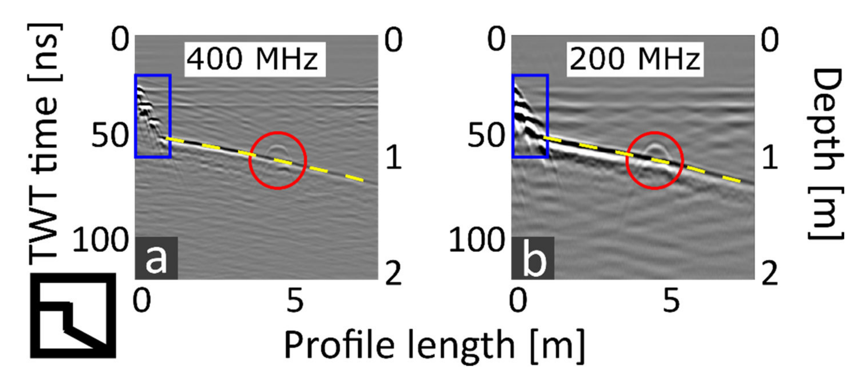
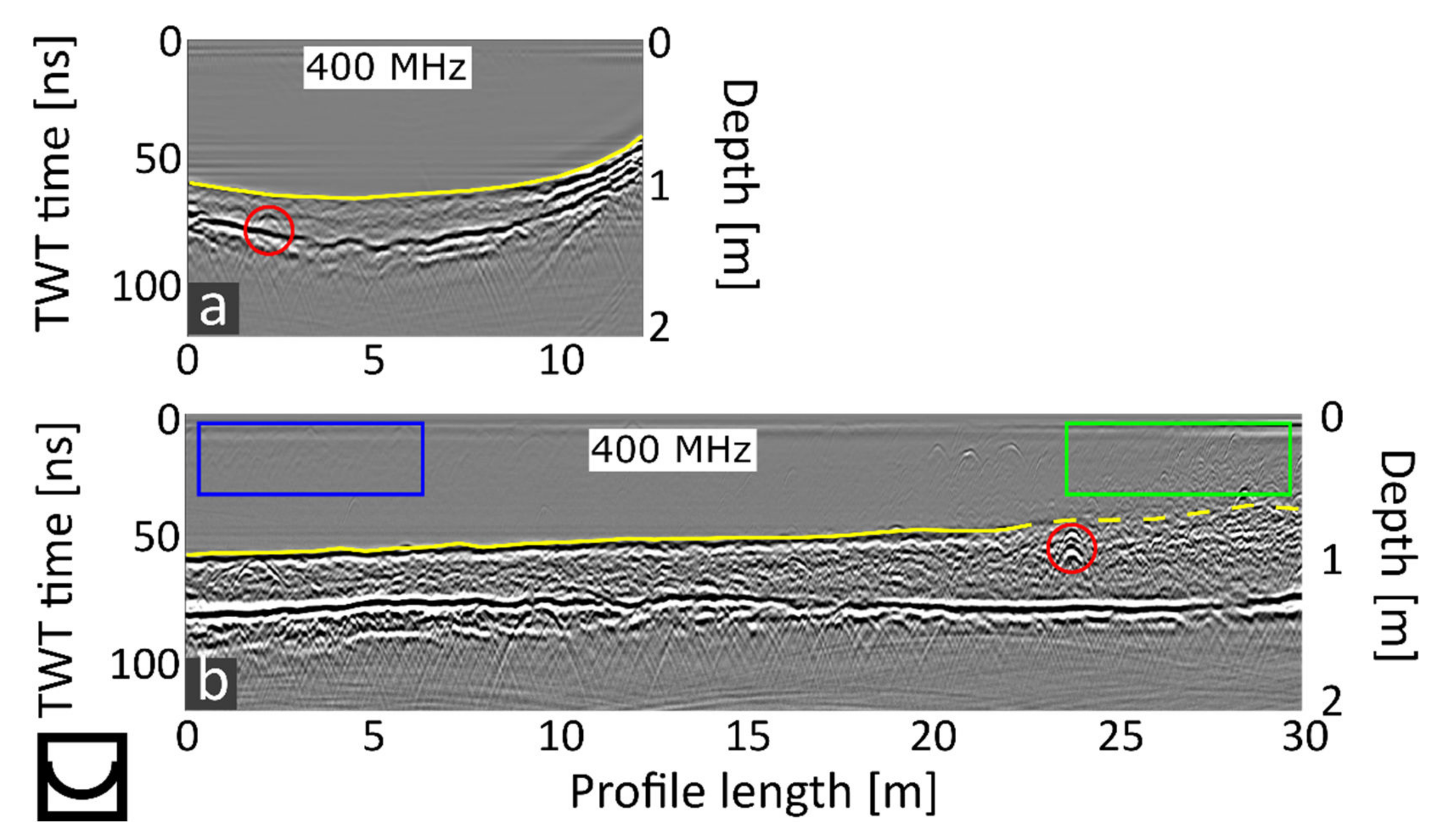
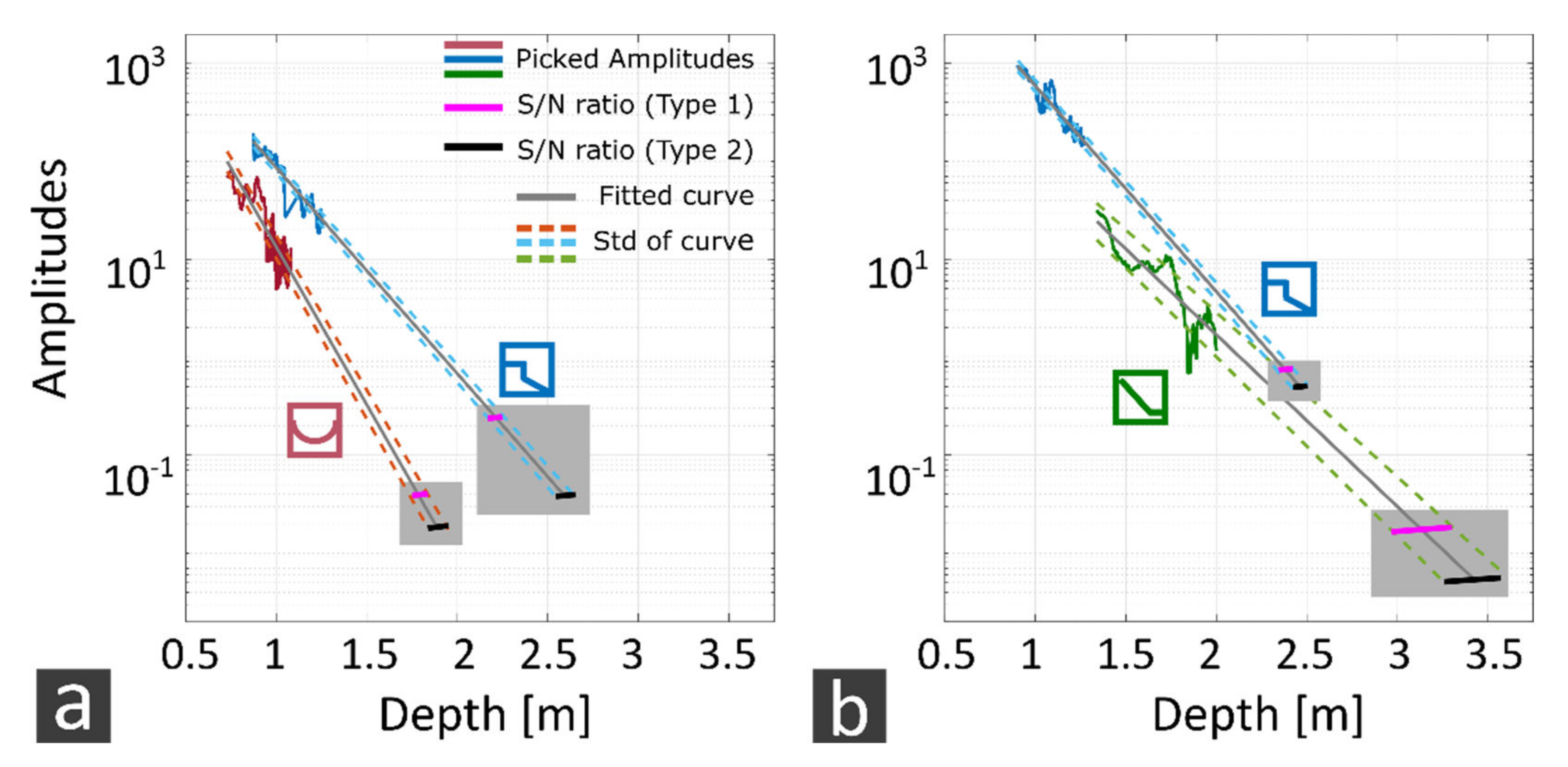
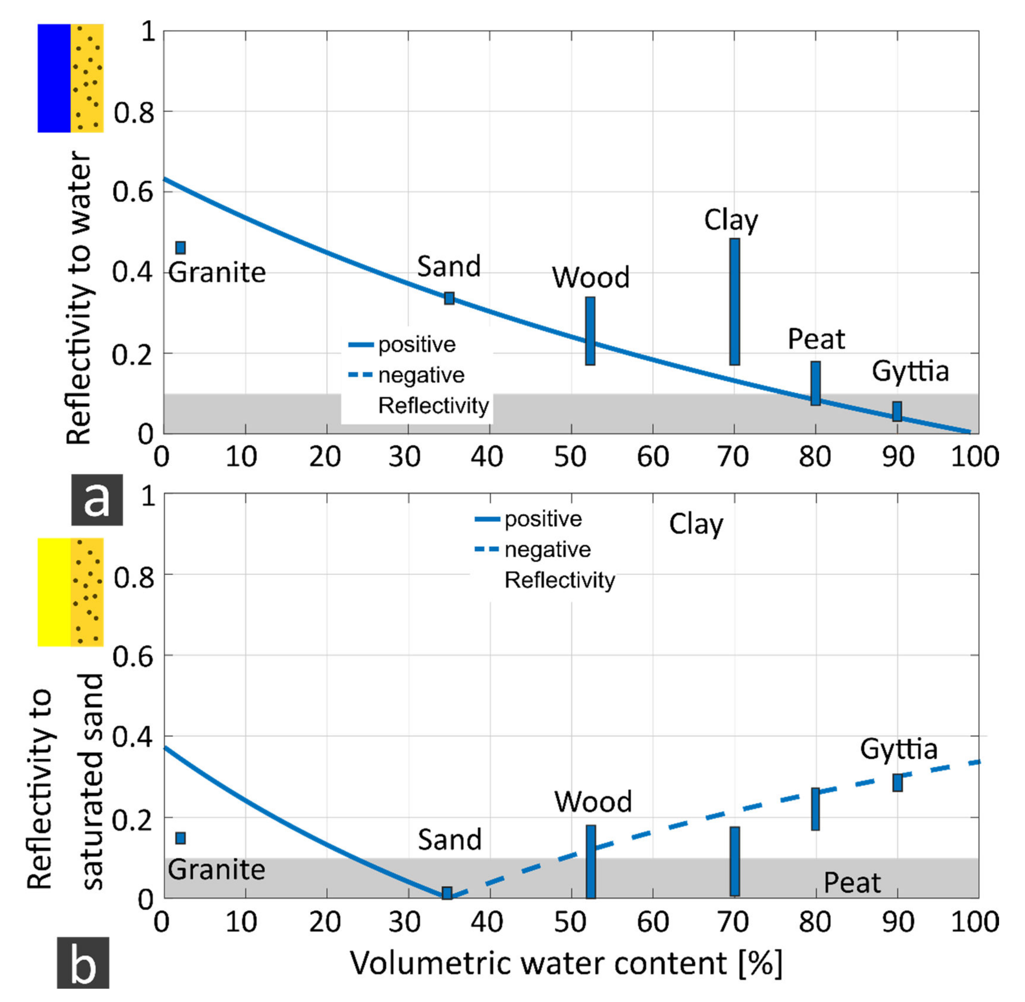
Table 1.
Comparison of water and soil properties and of the measurement setup for the GPR investigations at four different measurement locations: swimming pool, pond, river system, and flooded gravel pit.
Table 1.
Comparison of water and soil properties and of the measurement setup for the GPR investigations at four different measurement locations: swimming pool, pond, river system, and flooded gravel pit.
“Flooded Gravel Pit”  | “Swimming Pool”  | “River”  | “Pond”  | |
|---|---|---|---|---|
| Water column | Stagnant | Stagnant, | Flowing | Stagnant |
| vertical stratified | organic material | |||
| Ground material | Gravel | Tiles | Sand | Mud |
| Water depth | 1.2–5 m | 0.8–4 m | 0.2–0.4 m | 0.6–1.5 m |
| Water resistivity | 24.9 Ωm | 11.2 Ωm | ~17 Ωm | Unknown |
| Antenna | 400 and 200 MHz | 400 and 200 MHz | 400 and 200 MHz | 400 MHz |
| Stacking | 16 | 16 | 16 | 16 |
| Range | 240 ns | 120 ns | 120 ns | 120 ns |
| Number of samples | 822 | 411 | 411 | 411 |
| dt | 0.292 ns | 0.292 ns | 0.292 ns | 0.292 ns |
| Average wave velocity (according to diffraction hyperbolas in the water column) | 3.3 cm/ns | 3 cm/ns | 3 cm/ns | 3.3 cm/ns |
Table 2.
Physical parameters of dielectric permittivity and volumetric water content of the reference materials freshwater and saturated sand based on data from [21,43].
| Material | Relative Dielectric Permittivity | Volumetric Water Content (vol%) |
|---|---|---|
| Fresh water | 81 [43] | - |
| Saturated sand | 20 [21] | 45 [43] |
Table 3.
Physical parameters of dielectric permittivity and volumetric water content of the reference materials of different target materials. The values are based on data from [16,21,39,43].
| Material | Relative Dielectric Permittivity | Volumetric Water Content (vol%) |
|---|---|---|
| Rock matrix (quartz) | 4.2 | <1 |
| Clay | 10–40 | 50–85 |
| Peat | 40–60 | 70–95 |
| Gyttja | 60–70 | 90–95 |
| Wood | 20–40 | 50–60 |
| Granite | 8–11 | <2 |
Table 4.
Comparison of the attenuation coefficients for the measurement locations “flooded gravel pit”, “swimming pool”, and “pond”. They were determined based on field data using Equation (3) and additionally calculated with Equations (4) and (6).
Table 4.
Comparison of the attenuation coefficients for the measurement locations “flooded gravel pit”, “swimming pool”, and “pond”. They were determined based on field data using Equation (3) and additionally calculated with Equations (4) and (6).
| Location | α (Equation (3)) 400 MHz | α (Equations (4) and (6)) 400 MHz | α (Equation (3)) 200 MHz | α (Equations (4) and (6)) 200 MHz | |
|---|---|---|---|---|---|
| Flooded gravel pit |  | 1.75 | 1.9 | 2.02 | 1.1 |
| Swimming pool |  | 2.43 | 2.6 | 2.42 | 2.1 |
| Pond |  | 3.71 | - | - | - |
Table 5.
Comparison of the mean GPR signal/noise ratio type 1 (water ringing) and type 2 (common noise) of processed data at the measurement locations “pond”, “swimming pool”, “river”, and “flooded gravel pit”, and the antenna frequencies 200 and 400 MHz. The values are given in dB (10*log(S/NMean)).
| Location | S/N Type 1400 MHz | S/N Ratio Type 2400 MHz | S/N Ratio Type 1200 MHz | S/N Ratio Type 2200 MHz | |
|---|---|---|---|---|---|
| Flooded gravel pit |  | 13 dB | 38 dB | 19 dB | 27 dB |
| Swimming pool |  | 17 dB | 38 dB | 20 dB | 35 dB |
| River system |  | 33 dB | 68 dB | 39 dB | 60 dB |
| Pond |  | 33 dB | - | - |
Table 6.
Comparison of the constant parameter b (impact of the reflection coefficient and the antenna parameters on the depth penetration) and of the attenuation α, as well as of the maximum depth penetration and its standard deviation, for the 200 MHz and 400 MHz antennas from GSSI calculated from GPR profiles at three measurement locations.
| Location | −α·2 | Max. Depth Penetration (m) | Std. of Depth Penetration (m) | ||
|---|---|---|---|---|---|
| 400 MHz | |||||
| Pond |  | 10 | −7.4 | 1.9 | 0.06 |
| Swimming Pool |  | 9.3 | −4.8 | 2.6 | 0.05 |
| 200 MHz | |||||
| Swimming Pool |  | 11.2 | −4.8 | 2.5 | 0.06 |
| Flooded gravel pit |  | 8.6 | −4 | 3.5 | 0.18 |
Table 7.
The suitability of GPR for resolving contrasts between the materials freshwater, sand, clay, peat, gyttja, wood, granite, and brick. Material contrasts of are labeled with a check mark. When it might be that , the checkmarks are parenthesized. Material contrasts of show a cross.
Table 7.
The suitability of GPR for resolving contrasts between the materials freshwater, sand, clay, peat, gyttja, wood, granite, and brick. Material contrasts of are labeled with a check mark. When it might be that , the checkmarks are parenthesized. Material contrasts of show a cross.
| Fresh Water | Sand (Φ = 40%) | Clay | Peat | Gyttja | Wood | Granite | |
|---|---|---|---|---|---|---|---|
| Fresh water | ✓ | ✓ | (✓) | ✕ | ✓ | ✓ | |
| Sand | (✓) | ✓ | ✓ | (✓) | ✓ | ||
| Clay | (✓) | ✓ | (✓) | (✓) | |||
| Peat | (✓) | (✓) | ✓ | ||||
| Gyttja | ✓ | ✓ | |||||
| Wood | ✓ |
Publisher’s Note: MDPI stays neutral with regard to jurisdictional claims in published maps and institutional affiliations. |
© 2022 by the authors. Licensee MDPI, Basel, Switzerland. This article is an open access article distributed under the terms and conditions of the Creative Commons Attribution (CC BY) license (https://creativecommons.org/licenses/by/4.0/).
Share and Cite
MDPI and ACS Style
Fediuk, A.; Wunderlich, T.; Wilken, D.; Rabbel, W. Ground Penetrating Radar Measurements in Shallow Water Environments—A Case Study. Remote Sens. 2022, 14, 3659. https://0-doi-org.brum.beds.ac.uk/10.3390/rs14153659
AMA Style
Fediuk A, Wunderlich T, Wilken D, Rabbel W. Ground Penetrating Radar Measurements in Shallow Water Environments—A Case Study. Remote Sensing. 2022; 14(15):3659. https://0-doi-org.brum.beds.ac.uk/10.3390/rs14153659
Chicago/Turabian StyleFediuk, Annika, Tina Wunderlich, Dennis Wilken, and Wolfgang Rabbel. 2022. "Ground Penetrating Radar Measurements in Shallow Water Environments—A Case Study" Remote Sensing 14, no. 15: 3659. https://0-doi-org.brum.beds.ac.uk/10.3390/rs14153659
Note that from the first issue of 2016, this journal uses article numbers instead of page numbers. See further details here.