
Dual-Polarization Radar Fingerprints of Precipitation Physics: A Review
by
Matthew R. Kumjian
1,*, 
Olivier P. Prat
2,
Karly J. Reimel
1,
Marcus van Lier-Walqui
3 and
Hughbert C. Morrison
4 1
Department of Meteorology & Atmospheric Science, The Pennsylvania State University, University Park, PA 16801, USA
2
North Carolina Institute for Climate Studies, North Carolina State University, Asheville, NC 28801, USA
3
NASA Goddard Institute for Space Studies and Center for Climate Systems Research, Columbia University, New York, NY 10025, USA
4
National Center for Atmospheric Research, Boulder, CO 80305, USA
*
Author to whom correspondence should be addressed.
Remote Sens. 2022, 14(15), 3706; https://0-doi-org.brum.beds.ac.uk/10.3390/rs14153706
Submission received: 20 June 2022
/
Revised: 18 July 2022
/
Accepted: 27 July 2022
/
Published: 2 August 2022
(This article belongs to the Special Issue Radar-Based Studies of Precipitation Systems and Their Microphysics)
Abstract
:This article reviews how precipitation microphysics processes are observed in dual-polarization radar observations. These so-called “fingerprints” of precipitation processes are observed as vertical gradients in radar observables. Fingerprints of rain processes are first reviewed, followed by processes involving snow and ice. Then, emerging research is introduced, which includes more quantitative analysis of these dual-polarization radar fingerprints to obtain microphysics model parameters and microphysical process rates. New results based on a detailed rain shaft bin microphysical model are presented, and we conclude with an outlook of potentially fruitful future research directions.
1. Introduction
Dual-polarization radar observations are a valuable resource for studies of precipitation microphysics. The value of such observations arises by virtue of the information about hydrometeor shapes, sizes, orientations, and phase (liquid, ice) obtained through probing clouds and precipitation with two orthogonal polarizations (see, e.g., [1,2,3,4,5,6,7]).
Dual-polarization radar data have been widely and successfully used for a broad spectrum of applications. For example, there is a rich literature of studies developing and applying hydrometeor classification algorithms (HCAs), also referred to as hydrometeor identification or particle identification algorithms, which categorize individual pixels in graphical displays of radar data by the inferred dominant backscattering hydrometeor type. Such HCAs have been implemented using a variety of techniques, including theoretically or empirically determined thresholds for the different polarimetric radar variables that correspond to various hydrometeor types (e.g., [8,9,10]), fuzzy logic or neuro-fuzzy logic approaches (e.g., [1,11,12,13,14,15,16,17,18,19,20,21], among many others), and more data-driven approaches such as hierarchical clustering or support vector machines (e.g., [22,23,24,25,26], among many others). There is a good review of these approaches in [27]. While useful for spot-checking model distributions of hydrometeors (e.g., [28]), these types of HCAs provide only limited direct information about ongoing microphysical processes; one would have to infer processes from independent algorithmic classifications of nearby pixels. For example, a pixel classified as “snow aggregates” adjacent to one identified as “ice crystals” could imply aggregation, etc. In addition, HCAs often have different species categories than are used in models, making even such simple comparisons challenging (e.g., drizzle, different rainfall intensities, and “big drops” in HCAs compared to a single “rain category” in model microphysics schemes). Finally, although grounded in theoretical and empirical studies, there still exists uncertainty in the HCA classifications. As such, although HCAs are useful for qualitatively understanding the structure of precipitating systems, which can be leveraged for other applications such as rainfall estimation (e.g., [29]), other approaches should be considered for insights into microphysical processes.
There are also numerous studies proposing and applying retrievals of microphysically useful quantities from the dual-polarization radar variables. This includes estimates of precipitation rates (e.g., see the recent review in this collection [30]), raindrop size distribution parameters (e.g., [31,32,33]), ice water content and snow particle size distribution parameters [34,35,36,37,38,39]. These retrievals generally map the radar variables to important microphysical quantities through empirically or theoretically derived relationships. Such retrievals can be useful for comparisons to numerical model simulations because the retrieved quantities often are closely related to or directly predicted or diagnosed from model output. However, uncertainties in these types of retrievals often are unquantified, and many require a priori assumptions that introduce additional potential sources of error (e.g., [40]).
Instead, we focus this review on precipitation physics—processes—not hydrometeor classifications or retrievals. These physical processes are fundamental precipitation formation and evolution, yet their full understanding is lacking (e.g., [40]). An important, but often underemphasized, component of uncertainty in model-based studies of radar-observable signatures of microphysical processes is the fact that most do not consider uncertainties related to the simplifications and assumptions of the scheme. For example, bulk microphysics schemes treat a small number of size distribution moments prognostically, typically with some assumed underlying size distribution that can be uniquely determined from those prognostic moments [40]. This assumption allows for the precise and unique calculation of radar observables for a given set of moment values. However, such uniqueness does not exist in nature—for a given set of real precipitation moments, there are an infinite number of possible particle size distributions, each producing somewhat different values of radar observables. To better match nature, forward simulated radar observables should not be deterministic variables, but instead random variables that sample from an error distribution related to the variability that is not captured by the simplified state of the model microphysical assumptions. Indeed, this approach is taken in recent works and will be discussed in detail in later sections. By finding ways to quantitatively observe and characterize these ongoing processes with radar, while respecting these inherent uncertainties, we open the opportunity to learn more about them, and find robust ways to assess and improve model microphysics parameterizations.
We begin with an overview of the concept of microphysical fingerprints in dual-polarization radar observations, and then review the qualitative fingerprints for different precipitation processes. Then, we introduce some emerging research tackling more quantitative approaches to characterizing these microphysical fingerprints.
2. Qualitative Microphysical Fingerprints
The polarimetric radar variables used here include the radar reflectivity factor at horizontal polarization (ZH), differential reflectivity (ZDR), specific differential phase shift (KDP), and the co-polar correlation coefficient (ρhv). ZH is a measure of how much energy is scattered back to the radar, including from hydrometeors, insects, birds, etc. When these targets or particles are small compared to the radar wavelength, the amount of energy they scatter back to the radar is proportional to their horizontal dimension to the sixth power. The total ZH measured at a given location is the sum of this scattering from all particles within the radar pulse’s volume. As such, the total ZH is proportional to the number density of particles, as well. For a given particle size, those composed of liquid backscatter much greater power than those composed of ice; backscattered power from mixed-phase particles (i.e., those containing both liquid and ice) is somewhere between. ZV the radar reflectivity factor at vertical polarization, and is defined similarly, except it probes particles’ vertical dimensions. ZDR measures the difference between ZH and ZV (in logarithmic scale), and thus provides an indication of the particles’ shapes given that the particles are small compared to the radar wavelength. For example, an oblate raindrop with its maximum dimension oriented (on average) in the horizontal will backscatter more energy from the horizontally polarized radar signal than from the vertically polarized radar signal (i.e., ZH > ZV), leading to ZDR > 0 dB. Likewise, particles with more of their mass aligned in the vertical direction will have ZV > ZH, and thus ZDR < 0 dB. Spherical particles, or a collection of nonspherical particles that are randomly oriented, will scatter back energy equally at horizontal and vertical polarizations (ZH = ZV), resulting in ZDR = 0 dB. For a given non-spherical particle shape, those composed of liquid will produce larger magnitude ZDR values than those composed of ice, similar to the behavior of ZH. ZDR will be biased towards the particles in the radar sampling volume that dominate the backscattering because it is weighted by ZH and ZV.
Unlike ZH and ZDR, KDP is a measure of phase shift: it is the difference between the phases of the horizontally polarized and vertically polarized waves as they propagate through precipitation. Such phase differences arise from nonspherical particles: those with more of their mass aligned in the horizontal direction will produce KDP > 0 deg km−1, and those with more of their mass aligned in the vertical direction will produce KDP < 0 deg km−1. The sensitivity of KDP to drop size D is less than that of ZH, closer to ~D4 or ~D5 compared to the ~D6 dependence of ZH. KDP is also proportional to the number concentration of nonspherical particles. Unlike ZH and ZDR, KDP is insensitive to spherical particles; in a sense, it only “sees” the oriented nonspherical particles within the sampling volume. Finally, ρhv is a measure of the diversity of particles’ intrinsic ZDR within the sampling volume. For spherical particles or non-spherical particles with very similar shapes and orientations (and thus similar ZDR), ρhv is near unity. When there exists a variety of particle shapes and orientations in the sampling volume, ρhv is reduced. For a more detailed overview of the physical meaning of these quantities, see the texts [1,2,7] and the review series [3,4,5].
As precipitation falls towards Earth’s surface, a variety of physical processes may affect their sizes, spatial distribution, and phase. Such changes to particle populations are observable by polarimetric radars because of the sensitivities of the different radar variables to particle sizes, shapes, number densities, and physical compositions outlined above. Because these changes occur primarily as hydrometeors descend (i.e., outside of strong updrafts), vertical profiles of the polarimetric radar variables can be used to assess these ongoing processes. The idea of identifying polarimetric radar “fingerprints” of ongoing microphysical processes was introduced by [41], motivated by the interest in characterizing and quantifying microphysical processes in precipitation. Specifically, these fingerprints are defined as vertical changes in two or more of the dual-polarization radar variables within the lowest few kilometers of a precipitation shaft (e.g., increases in ZH and ZDR towards the ground). Use of multiple polarimetric radar variables provides additional degrees of freedom over conventional (i.e., ZH alone) observations, affording unique fingerprints for various microphysical processes. Such information provides an advantage over traditional techniques using ZH alone, such as contoured reflectivity by altitude diagrams (CFADs). These qualitative fingerprints are summarized in graphical form in [41], and reproduced with modifications in [7]. We will review these fingerprints associated with different microphysical processes here; their graphical depiction follows [42]. Figure 1 shows an example of how these fingerprints will be summarized graphically. The vertical axis represents height, and the abscissa indicates the value of the given polarimetric radar variable, each color coded and in individual subpanels. In the example shown, ZH, ZDR, and KDP all increase towards the ground.
2.1. Rain Microphysical Processes
Raindrops falling to Earth’s surface undergo a variety of processes, including interactions with other drops. The so-called collisional processes include collision-coalescence, and collisional breakup. Although these processes do not change the overall amount of raindrop mass in a rain shaft, they do redistribute the mass to different parts of the drop size distribution (DSD). As such, and because of the raindrop shape dependence on size, these processes have observable signals in the polarimetric radar measurements.
Collision-coalescence is the process by which two or more drops collide and stick together, or coalesce, to form a larger drop (e.g., [43]). As a result, the raindrop number concentration N decreases, but the overall mean raindrop size increases. For particles with sizes D much smaller than the radar’s wavelength, backscattering of the radar signal is a strong function of size (~D6), which dominates over backscattering’s direct proportionality to number concentration (~N). Therefore, collision-coalescence is expected to increase ZH in the rainshaft towards the ground, because the increase in drop size resulting from the merging of two or more drops dominates the decrease in number concentration of these smaller drops. Similarly, ZDR and KDP are both expected to increase towards the ground owing to the production of these larger, more oblate drops (Figure 2a). Using a detailed bin microphysical model, Ref. [44] first quantified the expected collision-coalescence fingerprint, revealing increases in ZH of <4 dB, in ZDR of <0.5 dB, and in KDP < 0.5 deg km−1 (at S band) over a 3-km, steady-state rain shaft.
Other collisions between raindrops result in a dramatically different outcome: the disruption or breakup of colliding drops into multiple, smaller drop fragments (e.g., [46,47]). Although the precise distribution of drop fragments following the collision between various drop-size pairs is highly complicated and still a subject of study (e.g., [48,49,50,51]), the overall effect on the polarimetric radar variables is understood. The increase in drop number concentration is overshadowed by the decrease in mean raindrop size, resulting in an observable effect of decreased ZH, ZDR, and KDP towards the ground (Figure 2b). The modeling study of [44] showed much larger changes in the radar variables owing to collisional breakup compared to collision-coalescence: decreases in magnitudes up to 5 dB for ZH, 1.5 dB for ZDR, and 0.7 deg km−1 for KDP (at S band) over the 3-km steady-state rain shaft. However, the authors noted that, based on comparisons to observations, the bin model’s accounting for collisional breakup may be “overaggressive,” leading to exaggerated vertical changes in the radar variables.
In nature, of course, collision-coalescence and collisional breakup do not act in isolation. Rather, both act on populations of raindrops simultaneously. Some regimes exist in which one process is dominant over the other, leading to observable fingerprints qualitatively consistent with those in Figure 2a,b. However, other regimes may exist in which both processes are approximately balanced, leading to relatively small vertical changes in the radar variables overall. In such cases, measurement errors may obfuscate the underlying fingerprint signal, making assessing the dominant microphysical process challenging, if not impossible.
When raindrops fall below cloud base into subsaturated air (i.e., relative humidity with respect to liquid water is <100%), they will lose mass owing to evaporation, defined as net vapor diffusion away from the drop and to the ambient environment. For vapor diffusion, the rate of change of raindrop size dD/dt is inversely proportional to the raindrop size D itself (e.g., [43]). In other words, smaller drops will lose size more rapidly owing to evaporation than larger drops. Given the strong size dependence of radar wave backscattering (for particles much smaller than the radar wavelength), evaporation can lead to a somewhat counterintuitive fingerprint in which ZH and KDP decrease towards the ground, but ZDR increases slightly (Figure 2c), as first pointed out by [52]. This occurs when the greater amount of mass lost from smaller drops relative to larger drops in a given DSD leads to a slight upward shift in the mean drop size. Using an idealized bin microphysics model, Ref. [53] showed that these increases in ZDR are quite small (<0.2 dB over a few-km-deep rainshaft) and likely within the measurement uncertainty of most polarimetric radars [54]. As such, careful averaging in space or time, or techniques such as quasi-vertical profiles [55] may be needed to observe this fingerprint robustly. In a follow-up study, Ref. [45] used a similar idealized model to demonstrate that the ZDR fingerprint can actually reverse, featuring ZDR decreasing towards the ground, in special cases of initial gamma DSDs (e.g., [56,57]) with large mean drop sizes (i.e., large ZDR at the top of the rain shaft) and large DSD breadth (Figure 3). However, Ref. [45] only considered evaporation, and ignored the collisional processes. Kumjian and Prat [44] showed that collisional breakup tends to dominate in rain shafts with such large initial ZDR; it is unclear if a pure evaporation signal could be observed given the propensity for such DSDs to undergo collisional breakup. The interplay between these processes requires detailed modeling; preliminary results of such modeling will be shown in a later section.
Unlike the collisional processes, net evaporation involves mass changing phases from liquid to vapor. This phase change is associated with diabatic cooling through the enthalpy of vaporization as the highest-energy water molecules escape the liquid drop, leaving behind lower-energy molecules and thus cooler drops overall (e.g., [43]). The authors of [45] used their idealized model to estimate the cooling rate in rain based on the observed fingerprint, and plausibly retrieved cooling rates on order of a few K hr−1. Use of polarimetric radar information to quantify thermodynamic changes in the environment is an exciting research frontier, and one that could lead to significant improvements in numerical models through, for example, data assimilation (e.g., [58]).
Because raindrop fall speed increases monotonically with increasing size up to a point before leveling off (e.g., [59,60]), differential sedimentation occurs. This is part of the reason why, as a cloud first begins to precipitate, one often encounters the largest drops at the ground first. However, this “size sorting” can be sustained in the presence of an updraft or non-zero storm-relative winds, which most often occur in environments with appreciable vertical wind shear (e.g., [61,62,63]). Because of the raindrop shape dependence on size, polarimetric radars are particularly well-suited for identifying regions of ongoing size sorting. These regions are observed as spatially offset enhancements of ZDR and ZH (and/or KDP); an iconic example is the “ZDR arc” feature offset from the precipitation core in supercell storms (e.g., [64,65,66,67]). For a rain shaft, the transient effect of size sorting is observed as a strong increase in ZDR towards the ground paired with decreases in ZH and KDP (Figure 2d; [44,61]). Although the fingerprint is qualitatively consistent with that of evaporation (cf. Figure 2c,d), the magnitude of the ZDR increase is far more significant for size sorting than for evaporation. Thus, in situations where size sorting and evaporation are both ongoing, it is expected that size sorting dominates the observed fingerprint.
To help visualize the different microphysical processes revealed by these fingerprints, [44] introduced a 4-quadrant parameter space (Figure 4) representing changes in different polarimetric radar variables. Plotting points representative of observed vertical gradients in the polarimetric variables (changes in ZH and ZDR towards the ground in the example shown in Figure 4) allows easy classification of the ongoing microphysical process. This rain microphysical fingerprint framework has found uses in the hydrometeorological literature, including classifying rainfall for quantitative precipitation estimation [68,69,70], and has recently been extended to similar work with satellite observations [71].
Here we apply the idea of fingerprinting to data collected during Hurricane Matthew, which made landfall on the United States in 2016. The storm produced a large stratiform precipitation shield over North Carolina, where the U.S. National Weather Service operational KRAX WSR-88D polarimetric radar near Raleigh was well-suited to observe the precipitation properties. We apply the QVP technique ([55]) to 11 h of data, starting at 13 UTC on 8 October 2016. During this time, the area around the KRAX radar experienced persistent rainfall as the Hurricane made landfall to the south, slowed, and eventually meandered eastward. Towards the end of this time period, drier air began wrapping around the west side of the storm, eroding the precipitation shield from west to east. Data below the melting layer (located > 4 km AGL) are selected to focus the analysis on rain microphysical processes. Figure 5a shows the time series of QVPs of ZH, revealing consistently moderate to heavy rain, with some times experiencing > 40 dBz at the lowest levels. Figure 5b is a similar presentation, but for ZDR. We note that, despite the larger ZH values, ZDR remains < 1 dB for much of the event, indicative of smaller drops (and expected based on the tropical nature of the precipitation).
To characterize the microphysical fingerprint observed in the data, we first extracted the vertical profiles of ZH and ZDR at each time and applied a 5-gate (~220-m) moving average filter to smooth the data. Then, a least-squares linear fit was computed for each data segment along a 15-gate (~660-m) moving window; the slope of these best-fit lines indicates the vertical gradients of ZH and ZDR. Next, these computed ZH and ZDR vertical gradients were used to assess the qualitative microphysical fingerprint. To avoid false classifications based on noise present in the data, we applied minimum thresholds of dZH/dz > 0.002 dB km−1 and dZDR/dz > 0.0001 dB km−1 (based on measurement uncertainties of 1–2 dB in ZH and 0.1–0.2 dB in ZDR cited in [54]).
The resulting fingerprint classifications are shown in Figure 5c. Despite some noisiness in the retrieval, an obvious feature is the prevalence of the coalescence fingerprint (54.4% of identified pixels). That coalescence should dominate the signal in tropical rainfall is expected based on the relatively small raindrop sizes (e.g., [44]). The breakup and “balance” fingerprints were identified in 19.3% and 15.7% of the pixels, respectively. Evaporation and/or size sorting was only identified in 10.6% of the pixels; interestingly, most of these occur after 19 UTC. Because of the spatial averaging involved in the QVP technique, one might not expect to see size sorting (which tends to be localized; see [61,62,63,64,65,66,67]) appear; indeed, the vertical gradients in ZDR after 19 UTC are small in magnitude. Recall that during this time, Hurricane Matthew was ingesting drier air from the west. Thus, this signal of increased prevalence of the evaporation fingerprint throughout this period is at least broadly consistent with the observed storm evolution.
As in this example, dual-polarization radar fingerprints have been used predominantly to infer (qualitatively) microphysical processes. It is unknown how process rate magnitudes vary throughout this parameters space, although one could hypothesize that the process rate magnitudes may increase with increasing fingerprint magnitude. For example, one could hypothesize a correlation between larger decreases (towards the ground) in ZH and ZDR and greater collisional breakup. As we will see later in Section 3, there is now some evidence that these fingerprints can be used for quantitative process rate information, which could substantially advance evaluation of numerical model microphysics schemes.
2.2. Snow and Ice Microphysical Processes
Similar to raindrops, ice crystals undergo a variety of microphysical processes during their existence and descent to the ground. Some of these processes involve collisions between hydrometeors, including ice–ice collisions that result in joining of two or more ice crystals (known as aggregation), ice–ice collisional fragmentation, and ice–cloud droplet collisions (known as riming). Further, ice particles may lose mass to the environment through net diffusion of vapor molecules away from the particle during sublimation. Unlike raindrops, however, ice particles may grow large enough entirely by vapor diffusion to sediment to the surface (e.g., [43]). The polarimetric radar fingerprints of these ice microphysical processes are far more challenging to characterize, owing in part to the myriad shapes that ice crystals may acquire during their lifetimes, as well as comparatively poor understanding of many of the processes involved in ice growth (see, e.g., [40]).
During vapor depositional growth of ice crystals, the particles may undergo substantial changes in shape. For example, a spherical cloud droplet may freeze and subsequently grow into an intricate dendritic snow crystal with aspect ratios that are extreme departures from unity [72,73]. During this growth, the particle gains mass from the surrounding vapor, increasing in size and thus increasing ZH. The aspect ratio’s growing departure from unity would suggest an increase in ZDR, because small, pristine ice crystals align themselves with maximum dimension in the horizontal, regardless of whether they take on oblate (e.g., plate-like) or prolate (e.g., needle-like) shapes [1,2,3,4,5,6,7]. However, ice crystal growth can be complicated by factors such as branching or hollowing (e.g., [74]). Such complicating factors may reduce the compactness of ice molecules in the particle, sometimes referred to as reducing the particle’s effective density, thereby contributing to a decrease in ZDR (see [75]). Which effect wins out? There is some observational evidence that pure vapor depositional growth for dendrites leads to approximately no change in ZDR, at least at X band (e.g., [76,77]). The lack of an observable sharp increase in ZDR during the very early growth from frozen droplets or other ice nuclei may be because the particle sizes were too small for the radar wavelength used. We speculate that, given a shorter radar wavelength sensitive to cloud-particle sizes, early growth should reflect a rapidly decreasing aspect ratio and thus increase in ZDR concurrent with an increase in ZH. For precipitation radar wavelengths (S, C, and X bands), this early growth likely is unobservable. KDP may respond similarly to ZDR, with the exception that a sufficiently large quantity of snow crystals would be necessary to obtain a strong enough signal to make a reliable estimate of KDP, particularly at longer wavelengths [76], given the much weaker scattering of ice particles compared to liquid and the inverse wavelength dependence of KDP [1,2]. Enhancements of KDP in the planar crystal growth region near −15 °C have been identified as a signal of vigorous vapor depositional growth (e.g., [78,79,80,81,82,83,84]). In contrast, others have argued that KDP enhancements represent the onset of aggregation (e.g., [85]). Some emerging evidence (Dunnavan et al., in preparation) suggests that primary nucleation and growth of large concentrations of ice crystals may be responsible for the observed KDP signal, consistent with the arguments put forth by [79]. Studies simulating the vapor depositional growth of ice crystals using reduced-density spheroids (e.g., [86,87]) are unable to capture the effects of snow crystal shape on electromagnetic scattering (e.g., [75]), and thus likely do not produce accurate fingerprints of vapor growth from ZDR and KDP. In summary, with considerable uncertainty, we suggest the fingerprint of vapor growth as increases in ZH, steady ZDR, and an increase in KDP accounting for primary nucleation and subsequent vapor growth of large concentrations of ice crystals (Figure 6a).
In contrast to vapor depositional growth, aggregation (defined as the collision of two or more ice particles and subsequent coagulation into a single, larger particle) leads to more readily understood polarimetric radar fingerprints. The increase in particle size dramatically increases ZH. Contrary to arguments that snow aggregates are well modeled by oblate spheroids (e.g., [89,90]), measurements of snow aggregate shapes reveal that they are highly irregular (e.g., [91,92]). However, their complicated and often chaotic orientations, paired with lower effective density, lead to ZDR values near 0 dB. Thus, the transition from pristine monomer ice crystals (particularly planar or columnar crystals) to well-developed aggregates comprising substantial numbers of monomer crystals (in other words, the snow aggregates often experienced in midlatitude snow storms that usually contain very large numbers of monomer ice crystals) is marked by a substantial decrease in ZDR. Note that, at temperatures below about −20 °C, ice crystal habits are complicated and not well understood [93]. These polycrystals, rosettes, and other irregular shapes have less extreme aspect ratios, and thus only moderate ZDR; for these cases, the aggregation fingerprint would be a more modest decrease in ZDR towards 0 dB (as seen in some cases from, e.g., [83]). In cases of very light aggregation (e.g., [76]), the resulting early aggregates with fewer constituent monomers may lead to positive ZDR values. Thus, the ZDR fingerprint of such light aggregation is still a decrease towards the ground, though this decrease may be less in magnitude than is typical in, for example, midlatitude snowstorms. Aggregation signatures for KDP are still subject to some debate in the scientific literature. As mentioned above, although some have argued the enhancement of KDP in the planar crystal growth region, constrained to temperatures near −15 °C, is a signal of the onset of aggregation [85], others have attributed this signature to vapor growth and/or nucleation. For the same reasons that well-developed snow aggregates produce near-zero ZDR values, KDP in snow aggregates also is near 0 deg km−1. Thus, any initial enhancement of KDP will decrease towards zero during ongoing aggregation. These are summarized in Figure 6b.
When an ice particle collects supercooled liquid cloud droplets, the droplets freeze on contact in a process known as riming. Because riming adds mass to the collector particle, ZH is expected to increase (though perhaps less substantially than aggregation, given the comparatively much smaller sizes of the collected cloud droplets). Evidence presented in [94] shows that ZDR could either increase or decrease as ice crystals become rimed, and that this ambiguous behavior may depend on the initial size (and, perhaps, the initial shape) of the crystals undergoing riming. However, the end result of heavy riming from a pristine crystal to a lump graupel particle is much like that of aggregation: increases in ZH and decreases in ZDR and KDP (Figure 6c). Riming can be complicated by other ongoing processes—for example, Hallett-Mossop rime splintering [95], which occurs at temperatures between about −3 and −8 °C and can lead to rapid vapor growth of columnar ice crystals in the same radar sampling volumes as the ongoing riming. In these cases, although ZH and ZDR tend to be dominated by the rimed particles (i.e., rimed aggregates or graupel), the large concentration of columnar ice crystals may lead to observable enhancements in KDP (Figure 6d), as shown in [83,96,97,98]. Kumjian et al. [97] argued that riming also leads to observable local decreases in the melting layer height, which they called “saggy bright bands”. However, subsequent modeling work by [99] suggested that heavier precipitation falling into the melting layer and associated increased cooling (owing to the enthalpy of melting) can lead to the development of an isothermal layer that is responsible for the sagging bright band (see the next subsection).
The impact of snow sublimation on the polarimetric radar variables has not received as much attention in the literature. However, a recent study by [88] has found repeatable signatures of dramatically reduced ZH and slightly reduced ZDR (usually no more than a few tenths of a dB, and likely often within the radar system’s noise) within sublimating, aggregated snow (Figure 6e). Intriguingly, they also found KDP enhancements at the bottom of the column, which they interpreted as sublimational fragmentation, a form of secondary ice production [100,101]. This represents another potential use of enhanced KDP to identify secondary ice production processes in clouds. Indeed, KDP is particularly well-suited for identifying secondary ice production given its strong sensitivity to the number concentration of highly anisotropic particles, and relatively low sensitivity to the larger particles that tend to dominate backscatter (e.g., snow aggregates, graupel).
Another unexpected but potentially useful signature was discovered in situations of refreezing of raindrops into ice pellets near the surface in winter precipitation [102]. The term “refreezing” has been used in the literature to distinguish the formation of ice pellets from, for example, droplet freezing in convective storm updrafts [103]. The intent is to imply the particles began as snow (ice), melted, and then froze into ice again, even though the term itself is imprecise from a physics perspective (much like “unmelting” would be). As raindrops freeze into ice pellets, the substantial decrease in relative permittivity was expected to drive down ZH, ZDR, and KDP. However, a local increase in ZDR (i.e., a local maximum) was observed within a broader layer of ZH decreasing towards the surface (Figure 6f). Kumjian et al. [102] proposed that preferential freezing of smaller drops led to the signature by increasing the relative contribution to ZH (and thus to ZDR) of the larger, unfrozen drops, analogous to evaporation and size sorting. They presented simple scattering calculations that supported this hypothesis. In contrast, Ref. [104] suggested that ice pellets acquired more exaggerated shapes owing to deformation during freezing (although no supporting calculations were provided). However, follow-up work by [105] using fully polarimetric Ka-band radar observations and modeling with scattering calculations by [106] have suggested that asymmetric freezing is the likely explanation for increasing ZDR. As a falling drop freezes, the upwind (downward-facing side) experiences much greater thermal energy transfer owing to the ventilation (e.g., [107]), and thus faster freezing. This asymmetry in ice shell thickness between the top and bottom of a freezing drop leads to an exaggerated aspect ratio for the inner, unfrozen liquid portion of the particle, increasing ZDR. A subtle increase in KDP is sometimes observed within the refreezing layer, and can also be explained by asymmetric freezing [106]. However, the presence of anisotropic crystals generated in the refreezing layer, which have been observed in at least some cases (e.g., [105,108]), could also lead to an increase in KDP as observed. Given the exaggerated particle shapes in the refreezing layer, as well as any additional particle shape deformations or other irregularities (e.g., [104]), ρhv also tends to decrease in the refreezing layer (not shown). Recently, Ref. [109] have suggested that refreezing of partially melted hydrometeors presents a different fingerprint, in which ZH, ZDR, and KDP all decrease towards the surface (indicated in Figure 6f by dashed lines). This is in part because a partially melted hydrometeor—one that contains ice—may start freezing immediately from the existing ice, rather than forming an ice shell that grows inward asymmetrically. This difference in geometries of the unfrozen liquid portion is argued to be responsible for the difference in observed fingerprints [109].
2.3. Melting of Snow and Ice
As ice hydrometeors reach portions of the atmosphere with wetbulb temperatures > 0 °C, they begin to melt. Owing to the much greater relative permittivity of liquid (compared to ice) at weather radar wavelengths, the melting particles’ backscattering properties change markedly during this transition: ZH increases and any polarization contrasts owing to nonspherical particle shapes become exaggerated. This can lead, for example, to large increases in ZDR and KDP, and decreases in ρhv (Figure 6g). The decreases in ρhv can be so dramatic that we have added a panel to Figure 6g to emphasize the importance in ρhv for identifying melting.
Such a marked transformation in the polarimetric radar fields is routinely observed in the melting layer of stratiform precipitation (e.g., [110]). Numerous studies have focused on melting layer detection (e.g., [111,112,113,114,115]). More recently, detailed statistical analyses of large datasets of melting layer observations have revealed insights into how processes above the melting layer (e.g., riming, vigorous depositional growth of planar crystals) are reflected in the melting layer properties and subsequent precipitation rates beneath the melting layer (e.g., [115,116]). Only [99], however, has attempted to extract quantitative information about microphysical process rates (specifically, cooling rates owing to melting) from the melting layer. Specifically, their simulations suggest a high correlation (r2 > 0.9) between the maximum KDP in the melting layer and the cooling rate.
The polarimetric radar signatures from melting hail and graupel are not as pronounced, owing to (i) a much larger range of fallspeeds for these particles as a function of their size, which tends to “spread out” the melting over a larger depth of the troposphere, and (ii) their shapes tend to be more regular than melting snowflakes. Nonetheless, melting of hail and graupel still leads to predictable increases in ZH and more exaggerated polarimetric contrasts. Several studies have coupled a microphysical model of melting hail by [117] with scattering calculations to produce expected melting hail signatures in terms of vertical profiles of the polarimetric radar variables (e.g., [118,119,120,121]). In particular, smaller (<2 cm) hailstones tend to acquire a “torus” of liquid meltwater that accumulates about their equator, stabilizing fall behaviors and leading to larger ZDR. In contrast, larger hail (>2 cm) tends to shed much of its meltwater. The lack of stabilization during fall leads to lower ZDR, on average, given the diversity of shapes found in natural hailstones [122]. This feature was exploited for an operational hail size discrimination algorithm ([121]) that classifies hail into three categories: sub-severe, severe, and significantly severe (<2.5 cm; 2.5 to 5.0 cm; and >5.0 cm, respectively; see [123] for proposed hail size naming conventions). However, none of this work has exploited the radar data for quantitative use in understanding hail processes; undoubtedly, interpretation is complicated by the myriad of natural hailstone shapes [122] as well as the significant uncertainty in fall behavior [124].
3. Emerging Research with Microphysical Fingerprints
More recently, efforts have started to analyze microphysical fingerprints in dual-polarization data more quantitatively, including with large sample sizes. This type of work is an important first step for robust statistical analyses of precipitation processes inferred from radar. Further, some of this work aims to quantify microphysical processes or process rates using information from the dual-polarization radar fingerprints described above. Here, we review a small sample of these recent and ongoing studies.
Reimel [42] explored the evolution of dominant rain fingerprints during a landfalling U.S. Hurricane. She found that a large fraction of fingerprints over the 12-h observation period suggested coalescence was dominant, in accord with expectations based on the tropical nature of the precipitation. Further, this study utilized the new Bayesian Observationally constrained Statistical-physical Scheme, or BOSS, model framework (e.g., [125,126]). BOSS is a warm-rain bulk microphysics parameterization scheme that is designed to allow constraint by dual-polarization radar observations. BOSS uses flexible microphysical process rate formulations, evolving raindrop size distribution moments using generalized power series that allows one to choose the number of terms used to describe a process, as well as the number of prognostic moments. BOSS was shown to reproduce the behavior of traditional microphysics schemes, while simultaneously allowing for robust quantification of uncertainty in parameter values as well as process rate formulations [125,126]. By using this framework, Ref. [42] was able to quantitatively analyze process rates in the radar-observed profiles, demonstrating that such process rate retrievals using radar observations are possible.
In addition, to process rate retrievals, classification techniques such as those used for HCAs are now being applied to vertical profiles of the polarimetric radar variables to characterize microphysical fingerprints. For example, Ref. [127] used an unsupervised classification method based on principal component analysis and k-means clustering to categorize fingerprints. The technique was able to identify some of the “textbook examples” of snow microphysics fingerprints, including those described above.
Recent work has demonstrated the ability of dual-polarization radar data to quantitatively retrieve important information in the context of bulk microphysics parameterization schemes, including uncertain microphysical parameters themselves. For example, Ref. [77] investigated the microphysical information content contained within dual-polarization radar fingerprints of vapor depositional growth of planar ice crystals. They used Markov chain Monte Carlo (MCMC) sampling within a Bayesian inference framework to estimate parameters in a bulk microphysics scheme. This method involved simultaneously perturbing 10 uncertain microphysical and kinematic model parameters, running the model, and evaluating the model output against the polarimetric radar observations. The process was repeated millions of times, resulting in an estimate of the full probability density function for each uncertain parameter, as well as parameter covariability [77]. In particular, the authors focused on faceted ice crystal growth during vapor deposition, following the parameterization of [128]. The simulations were constrained using X-band polarimetric radar observed vertical profiles of ZH and ZDR, along with vertically pointing Ka-band radar observations of mean Doppler velocity, taken during an Arctic mixed-phase cloud that produced pristine dendrites (a case analyzed by [76]). The resulting MCMC-constrained growth parameters produced values of differential growth rates along the “a” and “c” axes (along the basal and prism faces, respectively), equal to a temperature-dependent inherent growth ratio, Γ, times the ratio of the ice crystal c and a axis lengths, shown by purple dots in Figure 7. Detailed laboratory measurements and numerical simulations by [129] suggested that ice crystal facets grow at a rate equal to the ratio αc/αa, where αc and αa are the deposition coefficients along the a and c axes. Figure 7 also shows this ratio’s dependence on temperature and the associated uncertainty, extracted from wind tunnel measurements. The excellent correspondence between the radar-retrieved growth rates and wind tunnel measurements seen in Figure 7 demonstrates the quantitative microphysical information contained in dual-polarization radar fingerprints.
The technique also revealed relationships between dual-pol radar variables and the microphysical parameters in the model. For example, smaller simulated ZDR values were produced when the inherent growth ratio was larger, leading to crystals with less extreme aspect ratios and larger fall speeds ([77]). The authors made use of a probabilistic forward operator by [130] to better capture the natural variability of planar crystal shapes. Incredibly, the radar observations were informative to uncertain parameters in this probabilistic forward operator, as well: ZDR observations provided some constraint on the subbranch fractional coverage (a parameter determining the thickness of the dendritic ice crystal sub-branches).
As part of work towards a new parameterization for warm rain microphysics, known as BOSS [125,126], a large database of bin microphysical model simulations was compiled [131]. This database used the one-dimensional rainshaft model of [132,133], which explicitly treats the collisional processes and evaporation for a population of raindrops. Specifically, the bin model uses a number- and mass-conserving numerical scheme to solve the stochastic breakup and collection equations over 40 raindrop size (mass) bins. The bin model domain used was 3 km tall (10-m vertical grid spacing), with a 1 s timestep. Normalized gamma DSDs are initialized at the top of the domain, spanning median volume diameters from 0.2 mm to 4 mm, normalized intercept parameters ranging from 100 to 80,000 m−3 mm−1, and shape parameters ranging from −1 to 10, encompassing rainfall rates up to 500 mm hr−1. In all, this database comprises 9922 simulations featuring a wide parameter space of initial DSDs and rainfall rates (e.g., see [42,132] for additional details). As in [44], the dual-polarization radar variables were computed from the output of these bin model simulations, taking the final output time (t = 60 min) to obtain “steady state” rainshaft profiles. Vertical gradients in the polarimetric radar variables were computed at 299 height levels (corresponding to every 10 m in the vertical) in the domain, displayed in units of dB km−1 for ease of interpretation. Data points for which ZH ≥ 50 dBz were discarded as being unrealistically heavy rain. At each height level, the instantaneous process rates are obtained for the 0th and 6th DSD moments, hereafter M0 and M6, respectively, physically representing the total raindrop number concentration and radar reflectivity factor (in the small-particle scattering approximation). Given the clear relationship between M6 and the radar variables (e.g., see [134] for how each DSD moment is related to the dual-polarization radar variables), we will focus here on M6 process rates. Note that the results are sensitive to the bin model’s treatment of complex microphysical processes such as collisional breakup. Even though the bin model uses the state-of-the-art parameterizations of these processes, considerable uncertainty still exists e.g., [48,49,50,51,133]. Indeed, [44] suggested that the collisional breakup of drops in the bin model may be too aggressive, leading to more extreme collisional breakup fingerprint magnitudes than typically observed in rain. We therefore cautiously proceed with the analysis, given that the bin model and forward operator are the best available tools to quantitatively link process rate magnitudes and dual-polarization radar observables.
Figure 8 shows the [44] parameter space with points colored by their M6 collisional process rate, defined as the sum of the rate of change in M6 owing to coalescence (positive) and breakup (negative). The values are normalized on a 0 to 1 magnitude scale to facilitate comparison of different rainfall rates, etc. As such, the resulting positive or negative values indicate when one process wins out over the other: positive values indicate coalescence is dominating changes in M6 (which is closely related to ZH at S band), negative values indicate breakup is dominating changes in M6, and values near zero indicate a balance between these two processes. We can see that, in general, the breakup-dominated cases (negative values, purple dots) do fall within the “breakup” quadrant of the [44] parameter space, as expected. Likewise, the coalescence-dominated cases (green dots, positive values) are found mainly within the coalescence quadrant. Further, there is a tendency for stronger magnitudes of these processes to fall deeper within their respective quadrants, implying that the magnitudes of the radar fingerprints are related to the magnitudes of the process rates.
Figure 9 displays the same type of information, but this time for the M6 evaporation rate. Note that the process rate has been normalized and displayed between 0 and 1, such that 1 is the maximum evaporation rate. Recall that evaporation leads to a decrease in M6 (and thus ZH). The M6 evaporation rates exhibit large magnitudes in the “evaporation” quadrant, as well as the “breakup” quadrant. Interestingly, there is a clear shift of increasing magnitudes moving towards the top left within the cloud of points—in other words, even for points in the “breakup” quadrant, those closer to the evaporation quadrant of the [44] parameter space have larger M6 evaporation rate magnitudes. Further, the larger the breakup process rate magnitude, the larger the evaporation process rate magnitude, presumably because both scale with M6 and/or precipitation rate. Thus, even when evaporation does not dominate the observed changes in the dual-polarization radar fingerprints, information about the magnitude of evaporation is contained in the proximity to the evaporation quadrant, when displayed in the [44] parameter space diagram.
These simulations strongly suggest that the magnitudes of the dual-polarization radar fingerprints in rainshafts are quantitatively related to the microphysical process rates: larger magnitudes of the fingerprints imply larger normalized process rate magnitudes. This is promising, suggesting the use of dual-polarization radar data to not only infer ongoing microphysical processes, but to retrieve quantitative information about the process rates for direct comparisons with and evaluations of model microphysics schemes, and potentially, improved retrievals of cooling associated with evaporation (e.g., [45]).
It is clear from these results that, in most simulated (and presumably real) rainshafts, multiple microphysical processes may be ongoing, each affecting the resulting dual-polarization radar fingerprint. To dig deeper into the relative contributions of these processes, we computed the combined M6 process rate differences, defined as collisional processes minus evaporation. For this analysis, the “collisional processes” combine the magnitudes of both breakup and coalescence as “positive” contributors, and evaporation as a negative contributor. Thus, if evaporation dominates the changes to M6, the resulting “process rate difference” is negative; if collisional processes dominate over evaporation, the result is positive. Figure 10 shows the histograms of these combined M6 process rate differences (magenta dotted lines), categorized using the [44] quadrants. For example, if the simulated dual-polarization radar fingerprint suggests “coalescence,” the corresponding process rates are placed in the upper right quadrant. We did this for each of the 2,966,678 data points (see figure caption for numbers of data points in each quadrant). Further, Figure 10 also indicates which microphysical process dominates the contribution to the “collisional process rates” by overlaid lines: red indicating breakup dominates, blue indicating that coalescence dominates, and goldenrod indicating if coalescence and breakup are exactly balanced.
In the “evaporation/size sorting” quadrant (upper left in Figure 10), we see that evaporation dominates M6 for the vast majority of cases (82.6%), as expected; collisional processes dominate only 17.4% of cases there. Interestingly, of the cases for which evaporation dominates the overall changes to M6, coalescence is the dominant collisional process. In contrast, when collisional processes dominate in this quadrant, it is breakup that tends to win out. This makes physical sense because both evaporation and breakup should lead to decreases in ZH (and thus M6). For the majority of cases in which evaporation and coalescence are the dominant processes, ZDR tends to increase for both.
In contrast, the “coalescence” (upper right) quadrant in Figure 10 shows virtually no cases where evaporation dominates changes to M6 (only 2.3%). Of the 97.7% of cases for which collisional processes dominate, all of them feature coalescence as the dominant collisional process, in good agreement with the theoretical expectation of this quadrant ([44]). In essence, the coalescence fingerprint represents the “cleanest” or most unambiguous identification of a dominant ongoing process.
The “breakup” quadrant (lower left) in Figure 10 exhibits a markedly different behavior from the coalescence quadrant. In it, 55.3% of cases have evaporation dominating the M6 process rates, with only 44.7% of cases being dominated by collisional processes. Of those dominated by collisional processes, unsurprisingly, breakup is the overwhelmingly dominant process, again in good agreement with the theory. Note, however, that there are some coalescence-dominant cases in this quadrant, albeit with small process rate magnitudes. When evaporation dominates changes to M6 in this quadrant, there is a nearly equal mix of coalescence and breakup dominating the collisional processes.
Finally, in the “balance” quadrant (Figure 10, lower right), we see more than an order of magnitude fewer cases than in other quadrants. Further, 91.3% of the cases are dominated by collisional processes, with coalescence being the heavily favored process. Only 8.7% of cases in this quadrant have M6 changes dominated by evaporation.
This analysis reveals the complexity of multiple microphysical processes acting in a rainshaft. For instance, the coalescence fingerprint is relatively more certain than other fingerprints, given that almost all the cases in the “coalescence” quadrant (as defined by [44]) are indeed dominated by coalescence. Similarly, the “evaporation” quadrant is dominated by evaporation. In contrast, the breakup quadrant reveals that more than half the cases actually are evaporation dominated. Further, despite the much smaller number of fingerprints in the quadrant defined as “balance” by [44], we see that, in fact, coalescence tends to be the dominant process leading to this fingerprint. In other words, although collisional processes are dominant here (compared to evaporation), the distribution is heavily skewed in favor of coalescence, rather than being more balanced between coalescence and breakup.
Although process rate magnitudes and dual-polarization radar fingerprint magnitudes are indeed correlated, retrieval of quantitative process rate magnitudes may be challenging and requires careful sampling of the environment (e.g., to characterize the relative role of evaporation in modulating the observed fingerprints). Partitioning fingerprints into the [44] four-quadrant parameter space prior to such retrievals may provide additional constraint.
4. Concluding Remarks
Dual-polarization radar observations are powerful remote sensing data that provide both qualitative and quantitative information about ongoing microphysical processes in precipitation. This article reviews the concepts of qualitative radar-observed fingerprints of different microphysical processes, which are summarized in Table 1. We also explore the cutting-edge use of dual-polarization radar data to estimate important microphysical information quantitatively.
In our view, this emerging research into quantitative use of microphysical fingerprints is exciting, with ripe opportunity for fruitful studies. Making fuller use of all available information from polarimetric radars may help advance the science, too. For example, the co-polar correlation coefficient (ρhv) was neglected in most of the fingerprints discussed herein. In part, this is because the fingerprint work was originally developed for rain processes and using S-band radars, at which wavelength ρhv values tend to be very high (>0.98) for pure rain [3,7]. However, work [135] shows how some information may be gleaned from ρhv about the DSD shape (or “dispersion”) parameter, which controls the DSD breadth. Such information could potentially provide additional constraint for process rates that was not used for our BOSS work [125,126] Section 3. Linking this information about DSD breadth to generalized DSD moments, rather than to a specific parameter in an assumed underlying DSD functional form, may be particularly informative while simultaneously removing a major source of uncertainty [125,126,134]. Extracting this type of information from ρhv requires very high-quality measurements, however, and is likely only a capability of research-grade radars. Snow and ice processes are more challenging given the complexities of shapes. However, advances in scattering calculations [136] and microphysics schemes [40] should allow better realism in the representation of other processes for the coupled approach demonstrated above for rain and vapor depositional growth of ice. Incorporating ρhv into analyses of ice processes in a manner similar to [135] may also be valuable, particularly for aggregation and riming e.g., [84]. In this sense, the realm of ice microphysical processes guarantees fruitful advances. We advocate for Bayesian inference frameworks such as those used in [78,125,126] to consider all potential sources of uncertainty carefully and robustly. Doing so is crucial for critical evaluation of, and, ultimately, improvement of microphysics parameterizations in models of varying scales.
The information available from microphysical fingerprints can also be valuable for use in assimilation of polarimetric radar data into numerical models to improve analyses and forecasts of high-impact weather. Although assimilation of dual-polarization radar measurements into storm-scale numerical models has been explored, the results have been mixed [137,138,139,140]. This is in large part because many modern microphysics parameterization schemes predict quantities (e.g., raindrop or snowflake mass mixing ratio and number mixing ratio) that are not well-mapped to the radar measurements. Further, these model-predicted quantities are underpinned by necessary but rigid structural assumptions about particle size distributions built into the scheme that almost certainly are invalid in nature [134], meaning that natural variability is severely underrepresented [40,134,141]. Instead, using the dual-polarization radar fingerprints for information about process rates could be more fruitful, especially because these process rates can drive thermodynamic changes in precipitation systems that directly influence the system’s dynamics (e.g., evaporative cooling or ice particle melting driving storm cold pools). Such an approach may improve the connection between the imperfect model’s microphysical and dynamical processes. Some research along these lines [58] has shown encouraging results. Continued leveraging of dual-polarization radar observations for insights into microphysical processes is warranted, especially when combined with complementary information available from other observing platforms.
Author Contributions
Conceptualization, M.R.K. and K.J.R.; model simulations, O.P.P.; formal analysis, M.R.K.; data curation, O.P.P. and K.J.R.; writing—original draft preparation, M.R.K.; writing—review and editing, O.P.P., K.J.R., H.C.M. and M.v.L.-W.; visualization, M.R.K.; supervision, M.R.K.; funding acquisition, M.v.L.-W., M.R.K., H.C.M. and O.P.P. All authors have read and agreed to the published version of the manuscript.
Funding
Portions of this work were supported under previous grants from the U.S. Department of Energy Atmospheric System Research DE-SC0016579 and DE-SC0018933. The National Center for Atmospheric Research is sponsored by the National Science Foundation.
Data Availability Statement
Data from this study may be obtained by the first author.
Conflicts of Interest
The authors declare no conflict of interest. The funders had no role in the design of the study; in the collection, analyses, or interpretation of data; in the writing of the manuscript, or in the decision to publish the results.
References
- Doviak, R.J.; Zrnić, D.S. Doppler Radar and Weather Observations, 2nd ed.; Academic Press: Cambridge, MA, USA, 1993; 562p. [Google Scholar]
- Bringi, V.N.; Chandrasekar, V. Polarimetric Doppler Weather Radar: Principles and Applications; Cambridge University Press: Cambridge, UK, 2001; 636p. [Google Scholar]
- Kumjian, M.R. Principles and applications of dual-polarization weather radar. Part I: Description of the polarimetric radar variables. J. Oper. Meteor. 2013, 1, 226–242. [Google Scholar] [CrossRef]
- Kumjian, M.R. Principles and applications of dual-polarization weather radar. Part II: Warm-and cold-season applications. J. Oper. Meteor. 2013, 1, 243–264. [Google Scholar] [CrossRef]
- Kumjian, M.R. Principles and applications of dual-polarization weather radar. Part III: Artifacts. J. Oper. Meteor. 2013, 1, 265–274. [Google Scholar] [CrossRef]
- Kumjian, M.R. Weather radars. In Remote Sensing of Clouds and Precipitation, 1st ed.; Andronache, C., Ed.; Springer: Berlin/Heidelberg, Germany, 2018; pp. 15–63. [Google Scholar]
- Ryzhkov, A.V.; Zrnić, D.S. Radar Polarimetry for Weather Observations, 1st ed.; Springer: Berlin/Heidelberg, Germany, 2019; 486p. [Google Scholar]
- Straka, J.M.; Zrnić, D.S. An algorithm to deduce hydrometeor types and contents from multiparameter radar data. In Proceedings of the 26th International Conference on Radar Meteorology, Norman, OK, USA, 24–28 May 1993; American Meteorolpgical Society: Boston, MA, USA; pp. 513–516. [Google Scholar]
- Höller, H.; Hagen, M.; Meischner, P.F.; Bringi, V.N.; Hubbert, J. Life cycle and precipitation formation in a hybrid-type hailstorm revealed by polarimetric and Doppler radar measurements. J. Atmos. Sci. 1994, 51, 2500–2522. [Google Scholar] [CrossRef]
- Lopez, R.E.; Aubagnac, J.P. The lightning activity of a hailstorm as a function of changes in its microphysical characteristics inferred from polarimetric radar observations. J. Geophys. Res. 1997, 102, 16799–16813. [Google Scholar] [CrossRef] [Green Version]
- Vivekanandan, J.; Zrnić, D.S.; Ellis, S.M.; Oye, R.; Ryzhkov, A.V.; Straka, J. Cloud microphysics retrieval using S-band dual-polarization radar measurements. Bull. Am. Meteor. Soc. 1999, 80, 381–388. [Google Scholar] [CrossRef]
- Zrnić, D.S.; Ryzhkov, A.V. Polarimetry for weather surveillance radars. Bull. Am. Meteor. Soc. 1999, 80, 389–406. [Google Scholar] [CrossRef]
- Liu, H.; Chandrasekar, V. Classification of hydrometeors based on polarimetric radar measurements: Development of fuzzy logic and neuro-fuzzy systems, and in situ verification. J. Atmos. Oceanic Technol. 2000, 17, 140–164. [Google Scholar] [CrossRef]
- Zrnić, D.S.; Ryzhkov, A.; Straka, J.; Liu, Y.; Vivekanandan, J. Testing a procedure for automatic classification of hydrometeor types. J. Atmos. Oceanic Technol. 2001, 18, 892–913. [Google Scholar] [CrossRef]
- Lim, S.; Chandrasekar, V.; Bringi, V.N. Hydrometeor classification system using dual-polarization radar measurements: Model improvements and in situ verification. IEEE Trans. Geosci. Remote Sens. 2005, 43, 792–801. [Google Scholar] [CrossRef]
- Marzano, F.S.; Scaranari, D.; Vulpiani, G. Supervised fuzzy-logic classification of hydrometeors using C-band weather radars. IEEE Trans. Geosci. Remote Sens. 2007, 45, 3784–3799. [Google Scholar] [CrossRef]
- Park, H.S.; Ryzhkov, A.V.; Zrnić, D.S.; Kim, K.E. The hydrometeor classification algorithm for the polarimetric WSR-88D: Description and application to an MCS. Wea. Forecast. 2009, 24, 730–748. [Google Scholar] [CrossRef]
- Dolan, B.; Rutledge, S.A. A theory-based hydrometeor identification algorithm for X-band polarimetric radars. J. Atmos. Oceanic Technol. 2009, 26, 2071–2088. [Google Scholar] [CrossRef] [Green Version]
- Dolan, B.; Rutledge, S.A.; Lim, S.; Chandrasekar, V.; Thurai, M. A robust C-band hydrometeor identification algorithm and application to a long-term polarimetric radar dataset. J. Appl. Meteor. Climatol. 2013, 52, 2162–2186. [Google Scholar] [CrossRef]
- Al-Sakka, H.; Boumahmoud, A.A.; Fradon, B.; Frasier, S.J.; Tabary, P. A new fuzzy logic hydrometeor classification scheme applied to the French X-, C-, and S-band polarimetric radars. J. Appl. Meteor. Climatol. 2013, 52, 2328–2344. [Google Scholar] [CrossRef]
- Chen, Y.; Liu, X.E.; Bi, K.; Zhao, D. Hydrometeor Classification of Winter Precipitation in Northern China Based on Multi-Platform Radar Observation System. Remote Sens. 2021, 13, 5070. [Google Scholar] [CrossRef]
- Grazioli, J.; Tuia, D.; Berne, A. Hydrometeor classification from polarimetric radar measurements: A clustering approach. Atmos. Meas. Tech. 2015, 8, 149–170. [Google Scholar] [CrossRef] [Green Version]
- Besic, N.; Figueras i Ventura, J.; Grazioli, J.; Gabella, M.; Germann, U.; Berne, A. Hydrometeor classification through statistical clustering of polarimetric radar measurements: A semisupervised approach. Atmos. Meas. Tech. 2016, 9, 4425–4445. [Google Scholar] [CrossRef] [Green Version]
- Besic, N.; Gehring, J.; Praz, C.; Figueras i Ventura, J.; Grazioli, J.; Gabella, M.; Germann, U.; Berne, A. Unraveling hydrometeor mixtures in polarimetric radar measurements. Atmos. Meas. Tech. 2018, 11, 4847–4866. [Google Scholar] [CrossRef] [Green Version]
- Roberto, N.; Baldini, L.; Adirosi, E.; Facheris, L.; Cuccoli, F.; Lupidi, A.; Garzelli, A. A Support Vector Machine Hydrometeor Classification Algorithm for Dual-Polarization Radar. Atmosphere 2017, 8, 134. [Google Scholar] [CrossRef] [Green Version]
- Ribaud, J.F.; Machado, L.A.T.; Biscaro, T. X-band dual-polarization radar-based hydrometeor classification for Brazilian tropical precipitation systems. Atmos. Meas. Tech. 2019, 12, 811–837. [Google Scholar] [CrossRef] [Green Version]
- Lukach, M.; Dufton, D.; Crosier, J.; Hampton, J.M.; Bennett, L.; Neely, R.R. Hydrometeor classification of quasi-vertical profiles of polarimetric radar measurements using a top-down iterative hierarchical clustering method. Atmos. Meas. Tech. 2021, 14, 1075–1098. [Google Scholar] [CrossRef]
- Matsui, T.; Dolan, B.; Rutledge, S.A.; Tao, W.K.; Iguchi, T.; Barnum, J.; Lang, S.E. POLARRIS: A POLArimetric Radar Retrieval and Instrument Simulator. J. Geophys. Res. Atmos. 2019, 124, 4634–4657. [Google Scholar] [CrossRef] [Green Version]
- Giangrande, S.E.; Ryzhkov, A.V. Estimation of rainfall based on the results of polarimetric echo classification. J. Appl. Meteor. Climatol. 2008, 47, 2445–2462. [Google Scholar] [CrossRef]
- Ryzhkov, A.; Zhang, P.; Bukovčić, P.; Zhang, J.; Cocks, S. Polarimetric radar quantitative precipitation estimation. Remote Sens. 2022, 14, 1695. [Google Scholar] [CrossRef]
- Zhang, G.; Vivekanandan, J.; Brandes, E. A method for estimating rain rate and drop size distribution from polarimetric radar measurements. IEEE Trans. Geosci. Remote Sens. 2001, 39, 830–841. [Google Scholar] [CrossRef] [Green Version]
- Bringi, V.N.; Huang, G.J.; Chandrasekar, V.; Gorgucci, E. A Methodology for Estimating the Parameters of a Gamma Raindrop Size Distribution Model from Polarimetric Radar Data: Application to a Squall-Line Event from the TRMM/Brazil Campaign. J. Atmos. Oceanic Technol. 2002, 19, 633–645. [Google Scholar] [CrossRef] [Green Version]
- Gatidis, C.; Schleiss, M.; Unal, C. Sensitivity analysis of DSD retrievals from polarimetric radar in stratiform rain based on mu-lambda relationship. Atmos. Meas. Tech. 2022. in review. [Google Scholar] [CrossRef]
- Ryzhkov, A.V.; Zrnić, D.S.; Gordon, B.A. Polarimetric method for ice water content determination. J. Appl. Meteorol. 1998, 37, 125–134. [Google Scholar] [CrossRef]
- Lu, Y.; Aydin, K.; Cothiaux, E.E.; Verlinde, J. Retrieving cloud ice water content using millimeter- and centimeter wavelength radar polarimetric observables. J. Appl. Meteorol. Climatol. 2015, 54, 596–604. [Google Scholar] [CrossRef]
- Nguyen, C.M.; Wolde, M.; Korolev, A. Determination of ice water content (IWC) in tropical convective clouds from X-band dual-polarization airborne radar. Atmos. Meas. Tech. 2019, 12, 5897–5911. [Google Scholar] [CrossRef] [Green Version]
- Bukovčić, P.; Ryzhkov, A.; Zrnić, D.; Zhang, G. Polarimetric radar relations for quantification of snow based on disdrometer data. J. Appl. Meteor. Climatol. 2018, 57, 103–120. [Google Scholar] [CrossRef]
- Bukovčić, P.; Ryzhkov, A.; Zrnić, D. Polarimetric relations for snow estimation—Radar verification. J. Appl. Meteorol. Climatol. 2020, 59, 991–1009. [Google Scholar] [CrossRef] [Green Version]
- Bukovčić, P.; Ryzhkov, A.V.; Carlin, J.T. Polarimetric Radar Relations for Estimation of Visibility in Aggregated Snow. J. Atmos. Ocean. Technol. 2021, 38, 805–822. [Google Scholar] [CrossRef]
- Morrison, H.; van Lier-Walqui, M.; Fridlind, A.M.; Grabowski, W.W.; Harrington, J.Y.; Hoose, C.; Korolev, A.; Kumjian, M.R.; Milbrandt, J.A.; Pawlowska, H.; et al. Confronting the challenge of modeling cloud and precipitation microphysics. J. Adv. Model. Earth Syst. 2020, 12, e2019MS001689. [Google Scholar] [CrossRef]
- Kumjian, M.R. The Impact of Precipitation Physical Processes on the Polarimetric Radar Variables. Ph.D. Dissertation, The University of Oklahoma, Norman, OK, USA, 2012; 327p. Available online: https://hdl.handle.net/11244/319188 (accessed on 1 June 2022).
- Reimel, K.J. Leveraging Polarimetric Radar Observations to Learn about Rain Microphysics: An Exploration of Parameter Estimation, Uncertainty Quantification, and Observational Information Content with BOSS. Ph.D. Dissertation, The Pennsylvania State University, State College, PA, USA, 2021; 107p. Available online: https://etda.libraries.psu.edu/catalog/21872kjr50 (accessed on 1 June 2022).
- Lamb, D.; Verlinde, J. Physics and Chemistry of Clouds, 1st ed.; Cambridge University Press: Cambridge, UK, 2011; 584p. [Google Scholar] [CrossRef]
- Kumjian, M.R.; Prat, O.P. The impact of raindrop collisional processes on the polarimetric radar variables. J. Atmos. Sci. 2014, 71, 3052–3067. [Google Scholar] [CrossRef]
- Xie, X.; Evaristo, R.; Troemel, S.; Saavedra, P.; Simmer, C.; Ryzhkov, A. Radar observation of evaporation and implications for quantitative precipitation and cooling rate estimation. J. Atmos. Oceanic Technol. 2016, 33, 1779–1792. [Google Scholar] [CrossRef]
- Low, T.B.; List, R. Collision, coalescence, and breakup of raindrops. Part I: Experimentally established coalescence efficiencies and fragment size distributions in breakup. J. Atmos. Sci. 1982, 39, 1591–1606. [Google Scholar] [CrossRef] [Green Version]
- Low, T.B.; List, R. Collision, coalescence, and breakup of raindrops. Part II: Parameterization of fragment size distributions. J. Atmos. Sci. 1982, 39, 1607–1619. [Google Scholar] [CrossRef]
- Barros, A.P.; Prat, O.P.; Shrestha, P.; Testik, F.Y.; Bliven, L.F. Revisiting Low and List (1982): Evaluation of raindrop collision parameterizations using laboratory observations and modeling. J. Atmos. Sci. 2008, 65, 2983–2993. [Google Scholar] [CrossRef]
- Schlottke, J.; Straub, W.; Beheng, K.D.; Gomaa, H.; Weigand, B. Numerical investigation of collision induced breakup of raindrops. Part I: Methodology and dependencies on collision and eccentricity. J. Atmos. Sci. 2010, 67, 557–575. [Google Scholar] [CrossRef]
- Straub, W.; Beheng, K.D.; Seifert, A.; Schlottke, J.; Weigand, B. Numerical investigation of collision-induced breakup of raindrops. Part II: Parameterizations of coalescence efficiencies and fragment size distributions. J. Atmos. Sci. 2010, 67, 576–588. [Google Scholar] [CrossRef] [Green Version]
- Testik, F.Y.; Barros, A.P.; Bliven, L.F. Toward a physical characterization of raindrop collision outcomes. J. Atmos. Sci. 2011, 68, 1097–1113. [Google Scholar] [CrossRef] [Green Version]
- Li, X.; Srivastava, R.C. An analytical solution for raindrop evaporation and its application to radar rainfall measurements. J. Appl. Meteor. Climatol. 2001, 40, 1607–1616. [Google Scholar] [CrossRef]
- Kumjian, M.R.; Ryzhkov, A.V. The impact of evaporation on polarimetric characteristics of rain: Theoretical model and practical implications. J. Appl. Meteor. Climatol. 2010, 49, 1247–1267. [Google Scholar] [CrossRef] [Green Version]
- Ryzhkov, A.V.; Schuur, T.J.; Burgess, D.W.; Heinselman, P.L.; Giangrande, S.E.; Zrnić, D.S. The Joint Polarization Experiment: Polarimetric Rainfall measurements and hydrometeor classification. Bull. Am. Meteor. Soc. 2005, 86, 809–824. [Google Scholar] [CrossRef] [Green Version]
- Ryzhkov, A.V.; Zhang, P.; Reeves, H.; Kumjian, M.; Tschallener, T.; Trömel, S.; Simmer, C. Quasi-vertical profiles—A new way to look at polarimetric radar data. J. Atmos. Oceanic Technol. 2016, 33, 551–562. [Google Scholar] [CrossRef]
- Willis, P.T. Functional fits to some observed drop size distributions and parameterization of rain. J. Atmos. Sci. 1984, 41, 1648–1661. [Google Scholar] [CrossRef] [Green Version]
- Testud, J.; Oury, S.; Black, R.A.; Amayenc, P.; Dou, X. The concept of “normalized” distribution to describe raindrop spectra: A tool for cloud physics and cloud remote sensing. J. Appl. Meteor. 2001, 40, 1118–1140. [Google Scholar] [CrossRef]
- Carlin, J.T.; Gao, J.; Snyder, J.C.; Ryzhkov, A.V. Assimilation of ZDR columns for improving the spinup and forecast of convective storms in storm-sclae models: Proof-of-concept experiments. Mon. Wea. Rev. 2017, 145, 5033–5057. [Google Scholar] [CrossRef]
- Brandes, E.A.; Zhang, G.; Vivekanandan, J. Experiments in rainfall estimation with a polarimetric radar in a subtropical environment. J. Appl. Meteor. 2002, 41, 674–685. [Google Scholar] [CrossRef] [Green Version]
- Thurai, M.; Huang, G.J.; Bringi, V.N.; Randeu, W.L.; Schönhuber, M. Drop shapes, model comparisons, and calculations of polarimetric radar parameters in rain. J. Atmos. Oceanic Technol. 2007, 24, 1019–1032. [Google Scholar] [CrossRef]
- Kumjian, M.R.; Ryzhkov, A.V. The impact of size sorting on the polarimetric radar variables. J. Atmos. Sci. 2012, 69, 2042–2060. [Google Scholar] [CrossRef]
- Dawson, D.T.; Mansell, E.R.; Kumjian, M.R. Does wind shear cause hydrometeor size sorting? J. Atmos. Sci. 2015, 72, 340–348. [Google Scholar] [CrossRef]
- Loeffler, S.D.; Kumjian, M.R. Idealized model simulations to determine impacts of storm-relative winds on differential reflectivity and specific differential phase fields. J. Geophys. Res. Atmos. 2020, 125, e2020JD033870. [Google Scholar] [CrossRef]
- Kumjian, M.R.; Ryzhkov, A.V. Polarimetric signatures in supercell thunderstorms. J. Appl. Meteor. Climatol. 2008, 47, 1940–1961. [Google Scholar] [CrossRef]
- Kumjian, M.R.; Ryzhkov, A.V. Storm-relative helicity revealed from polarimetric radar measurements. J. Atmos. Sci. 2009, 66, 667–685. [Google Scholar] [CrossRef] [Green Version]
- Loeffler, S.D.; Kumjian, M.R.; Jurewicz, M.; Frech, M.M. Differentiating between tornadic and nontornadic supercells using polarimetric radar signatures of hydrometeor size sorting. Geophys. Res. Lett. 2020, 47, e2020GL088242. [Google Scholar] [CrossRef]
- Wilson, M.B.; Van Den Broeke, M.S. An automated python algorithm to quantify ZDR arc and KDP-ZDR separation signatures in supercells. J. Atmos. Oceanic Technol. 2021, 38, 371–386. [Google Scholar] [CrossRef]
- Carr, N.; Kirstetter, P.E.; Gourley, J.J.; Hong, Y. Polarimetric Signatures of Midlatitude Warm-Rain Precipitation Events. J. Appl. Meteor. Climatol. 2017, 56, 697–711. [Google Scholar] [CrossRef]
- Porcacchia, L.; Kirstetter, P.E.; Gourley, J.J.; Maggioni, V.; Cheong, B.L.; Anagnostou, M.N. Toward a Polarimetric Radar Classification Scheme for Coalescence-Dominant Precipitation: Application to Complex Terrain. J. Hydrometeor. 2017, 18, 3199–3215. [Google Scholar] [CrossRef]
- Erlingis, J.M.; Gourley, J.J.; Kirstetter, P.E.; Anagnostou, E.N.; Kalogiros, J.; Anagnostou, M.N.; Petersen, W. Evaluation of Operational and Experimental Precipitation Algorithms and Microphysical Insights during IPHEx. J. Hydrometeor. 2018, 19, 113–125. [Google Scholar] [CrossRef]
- Porcacchia, L.; Kirstetter, P.E.; Maggioni, V.; Tanelli, S. Investigating the GPM Dual-frequency Precipitation Radar signatures of low-level precipitation enhancement. Quart. J. Roy. Meteor. Soc. 2019, 145, 3161–3174. [Google Scholar] [CrossRef]
- Libbrecht, K.G. The physics of snow crystals. Rep. Prog. Phys. 2005, 68, 855–895. [Google Scholar] [CrossRef] [Green Version]
- Harrington, J.Y.; Sulia, K.; Morrison, H. A method for adaptive habit prediction in bulk microphysical models. Part I: Theoretical development. J. Atmos. Sci. 2013, 70, 349–364. [Google Scholar] [CrossRef]
- Nelson, J.; Knight, C. Snow crystal habit changes explained by layer nucleation. J. Atmos. Sci. 1998, 55, 1452–1465. [Google Scholar] [CrossRef] [Green Version]
- Schrom, R.S.; Kumjian, M.R. Bulk-density representations of branched planar ice crystals: Errors in the polarimetric radar variables. J. Appl. Meteor. Climatol. 2018, 57, 333–346. [Google Scholar] [CrossRef]
- Oue, M.; Galletti, M.; Verlinde, J.; Ryzhkov, A.; Lu, Y. Use of X-band differential reflectivity measurements to study shallow Arctic mixed-phase clouds. J. Appl. Meteor. Climatol. 2016, 55, 403–424. [Google Scholar] [CrossRef]
- Schrom, R.S.; van Lier-Walqui, M.; Kumjian, M.R.; Harrington, J.Y.; Jensen, A.A.; Chen, Y.S. Radar-based Bayesian estimation of ice crystal growth parameters within a microphysical model. J. Atmos. Sci. 2021, 78, 549–569. [Google Scholar] [CrossRef]
- Kennedy, P.C.; Rutledge, S.A. S-band dual-polarization radar observations of winter storms. J. Appl. Meteor. Climatol. 2011, 50, 844–858. [Google Scholar] [CrossRef]
- Andrić, J.; Kumjian, M.R.; Zrnić, D.S.; Straka, J.M.; Melnikov, V.M. Polarimetric signatures above the melting layer in winter storms: An observational and modeling study. J. Appl. Meteor. Climatol. 2013, 52, 682–700. [Google Scholar] [CrossRef]
- Bechini, R.; Baldini, L.; Chandrasekar, V. Polarimetric radar observations in the ice region of precipitation clouds at C-band and X-band radar frequencies. J. Appl. Meteor. Climatol. 2013, 52, 1147–1169. [Google Scholar] [CrossRef]
- Schrom, R.S.; Kumjian, M.R.; Lu, Y. Polarimetric radar signatures of dendritic growth zones within Colorado winter storms. J. Appl. Meteor. Climatol. 2015, 54, 2365–2388. [Google Scholar] [CrossRef]
- Schrom, R.S.; Kumjian, M.R. Connecting microphysical processes in Colorado winter storms with vertical profiles of radar observations. J. Appl. Meteor. Climatol. 2016, 55, 1771–1787. [Google Scholar] [CrossRef]
- Kumjian, M.R.; Lombardo, K.A. Insights into the evolving microphysical and kinematic structure of northeastern U.S. winter storms from dual-polarization Doppler radar. Mon. Wea. Rev. 2017, 145, 1033–1061. [Google Scholar] [CrossRef] [Green Version]
- Griffin, E.M.; Schuur, T.J.; Ryzhkov, A.V. A polarimetric analysis of ice microphysical processes in snow using quasi-vertical profiles. J. Appl. Meteor. Climatol. 2018, 57, 31–50. [Google Scholar] [CrossRef]
- Moisseev, D.N.; Lautaportti, S.; Tyynela, J.; Lim, S. Dual-polarization radar signatures in snowstorms: Role of snowflake aggregation. J. Geophys. Res. Atmos. 2015, 120, 12644–12655. [Google Scholar] [CrossRef] [Green Version]
- Sulia, K.J.; Kumjian, M.R. Simulated polarimetric fields of ice vapor growth using the adaptive habit model. Part I: Large-eddy simulations. Mon. Wea. Rev. 2017, 145, 2281–2302. [Google Scholar] [CrossRef]
- Sulia, K.J.; Lebo, Z.J.; Przybylo, V.M.; Schmitt, C.G. A new method for ice-ice aggregation in the adaptive habit model. J. Atmos. Sci. 2021, 78, 133–154. [Google Scholar] [CrossRef]
- Carlin, J.; Reeves, H.D.; Ryzhkov, A.V. Polarimetric observations and simulations of sublimating snow: Implications for nowcasting. J. Appl. Meteor. Climatol. 2021, 60, 1035–1054. [Google Scholar] [CrossRef]
- Ryzhkov, A.; Pinsky, M.; Pokrovsky, A.; Khain, A. Polarimetric radar observation operator for a cloud model with spectral microphysics. J. Appl. Meteor. Climatol. 2011, 50, 873–894. [Google Scholar] [CrossRef]
- Garrett, T.J.; Yuter, S.E.; Fallgatter, C.; Shkurko, K.; Rhodes, S.R.; Endries, J.L. Orientations and aspect ratios of falling snow. Geophys. Res. Lett. 2015, 42, 4617–4622. [Google Scholar] [CrossRef]
- Dunnavan, E.L.; Jiang, Z. A general method for estimating bulk 2D projections of ice particle shape: Theory and applications. J. Atmos. Sci. 2019, 76, 305–332. [Google Scholar] [CrossRef]
- Dunnavan, E.L.; Jiang, Z.; Harrington, J.Y.; Verlinde, J.; Fitch, K.; Garrett, T.J. The shape and density evolution of snow aggregates. J. Atmos. Sci. 2019, 76, 3919–3940. [Google Scholar] [CrossRef]
- Bailey, M.P.; Hallett, J. A comprehensive habit diagram for atmospheric ice crystals: Confirmation from the laboratory, AIRS II, and other field studies. J. Atmos. Sci. 2009, 66, 2888–2899. [Google Scholar] [CrossRef] [Green Version]
- Moisseev, D.; von Lerber, A.; Tiira, J. Quantifying the effect of riming on snowfall using ground-based observations. J. Geophys. Res. Atmos. 2018, 122, 4019–4037. [Google Scholar] [CrossRef] [Green Version]
- Hallett, J.; Mossop, S.C. Production of secondary ice particles during the riming process. Nature 1974, 249, 26–28. [Google Scholar] [CrossRef]
- Grazioli, J.; Lloyd, G.; Panziera, L.; Hoyle, C.R.; Connolly, P.J.; Henneberger, J.; Berne, A. Polarimetric radar and in situ observations of riming and snowfall microphysics during CLACE 2014. Atmos. Chem. Phys. 2015, 15, 13787–13802. [Google Scholar] [CrossRef] [Green Version]
- Kumjian, M.R.; Mishra, S.; Giangrande, S.E.; Toto, T.; Ryzhkov, A.V.; Bansemer, A. Polarimetric radar and aircraft observations of saggy bright bands during MC3E. J. Geophys. Res. Atmos. 2016, 121, 3584–3607. [Google Scholar] [CrossRef] [Green Version]
- Sinclair, V.A.; Moisseev, D.; von Lerber, A. How dual-polarization radar observations can be used to verify model representation of secondary ice. J. Geophys. Res. Atmos. 2016, 121, 10954–10970. [Google Scholar] [CrossRef] [Green Version]
- Carlin, J.T.; Ryzhkov, A.V. Estimation of melting-layer cooling rate from dual-polarization radar: Spectral bin model simulations. J. Appl. Meteor. Climatol. 2019, 58, 1485–1508. [Google Scholar] [CrossRef]
- Oraltay, R.G.; Hallett, J. Evaporation and melting of ice crystals: A laboratory study. Atmos. Res. 1989, 24, 169–189. [Google Scholar] [CrossRef]
- Korolev, A.; Heckman, I.; Wolde, M.; Ackerman, A.S.; Fridlind, A.M.; Ladino, L.A.; Lawson, R.P.; Milbrandt, J.; Williams, E. A new look at the environmental conditions favorable to secondary ice production. Atmos. Chem. Phys. 2020, 20, 1391–1429. [Google Scholar] [CrossRef]
- Kumjian, M.R.; Ryzhkov, A.V.; Reeves, H.D.; Schuur, T.J. A dual-polarization radar signature of hydrometeor refreezing in winter storms. J. Appl. Meteor. Climatol. 2013, 52, 2549–2566. [Google Scholar] [CrossRef]
- Kumjian, M.R.; Ganson, S.M.; Ryzhkov, A.V. Freezing of raindrops in deep convective updrafts: A microphysical and polarimetric model. J. Atmos. Sci. 2012, 69, 3471–3490. [Google Scholar] [CrossRef]
- Nagumo, N.; Adachi, A.; Yamauchi, H. Geometrical properties of hydrometeors during the refreezing process and their effects on dual-polarized radar signals. Mon. Wea. Rev. 2019, 147, 1753–1768. [Google Scholar] [CrossRef]
- Kumjian, M.R.; Tobin, D.M.; Oue, M.; Kollias, P. Microphysical insights into ice pellet formation revealed by fully polarimetric Ka-band Doppler radar. J. Appl. Meteor. Climatol. 2020, 59, 1557–1580. [Google Scholar] [CrossRef]
- Tobin, D.M.; Kumjian, M.R. Microphysical and polarimetric radar modeling of hydrometeor refreezing. J. Atmos. Sci. 2021, 78, 1965–1981. [Google Scholar] [CrossRef]
- Murray, W.A.; List, R. Freezing of water drops. J. Glaciol. 1972, 11, 415–429. [Google Scholar] [CrossRef] [Green Version]
- Stewart, R.E.; Crawford, R.W. Some characteristics of the precipitation formed within winter storms over eastern Newfoundland. Atmos. Res. 1995, 36, 17–37. [Google Scholar] [CrossRef]
- Tobin, D.M.; Kumjian, M.R.; Oue, M.; Kollias, P. Refreezing of partialy melted hydrometeors: Polarimetric radar observations and microphysical model simulations. J. Atmos. Sci. 2022. in preparation. [Google Scholar]
- Zrnić, D.S.; Balakrishnan, N.; Ziegler, C.S.; Bringi, V.N.; Aydin, K.; Matejka, T. Polarimetric signatures in the stratiform region of a mesoscale convective system. J. Appl. Meteor. 1993, 32, 678–693. [Google Scholar] [CrossRef]
- Brandes, E.A.; Ikeda, K. Freezing-level estimation with polarimetric radar. J. Appl. Meteor. 2004, 43, 1541–1553. [Google Scholar] [CrossRef]
- Baldini, L.; Gorgucci, E. Identification of the melting layer through dual-polarization radar measurements at vertical incidence. J. Atmos. Oceanic Technol. 2006, 23, 829–839. [Google Scholar] [CrossRef]
- Matrosov, S.Y.; Clark, K.A.; Kingsmill, D.E. A polarimetric radar approach to identify rain, melting-layer, and snow regions for applying corrections to vertical profiles of reflectivity. J. Appl. Meteorol. Clim. 2007, 46, 154–166. [Google Scholar] [CrossRef]
- Giangrande, S.E.; Krause, J.M.; Ryzhkov, A.V. Automatic designation of the melting layer with a polarimetric prototype of the WSR-88D radar. J. Appl. Meteorol. Clim. 2008, 47, 1354–1364. [Google Scholar] [CrossRef]
- Wolfensberger, D.; Scipion, D.; Berne, A. Detection and characterization of the melting layer based on polarimetric radar scans. Quart. J. Roy. Meteor. Soc. 2016, 142, 108–124. [Google Scholar] [CrossRef]
- Troemel, S.R.; Ryzhkov, A.V.; Hickman, B.; Mühlbauer, K.; Simmer, C. Polarimetric radar variables in the layers of melting and dendritic growth at X ban—implications for a nowcasting strategy in stratiform rain. J. Appl. Meteor. Climatol. 2019, 58, 2497–2522. [Google Scholar] [CrossRef]
- Rasmussen, R.M.; Heymsfield, A.J. Melting and shedding of graupel and hail. Part I: Model physics. J. Atmos. Sci. 1987, 44, 2754–2763. [Google Scholar] [CrossRef] [Green Version]
- Vivekanandan, J.; Bringi, V.N.; Raghavan, R. Multiparameter radar modeling and observation of melting ice. J. Atmos. Sci. 1990, 47, 549–564. [Google Scholar] [CrossRef] [Green Version]
- Meischner, P.F.; Bringi, V.N.; Heimann, D.; Höller, H. A squall line in southern Germany: Kinematics and precipitation formation as deduced by advanced polarimetric and Doppler radar measurements. Mon. Wea. Rev. 1991, 119, 678–701. [Google Scholar] [CrossRef] [Green Version]
- Ryzhkov, A.V.; Kumjian, M.R.; Ganson, S.M.; Khain, A.P. Polarimetric radar characteristics of melting hail. Part I: Theoretical simulations using spectral microphysical modeling. J. Appl. Meteor. Climatol. 2013, 52, 2849–2870. [Google Scholar] [CrossRef]
- Ryzhkov, A.V.; Kumjian, M.R.; Ganson, S.M.; Zhang, P. Polarimetric radar characteristics of melting hail. Part II: Practical Implications. J. Appl. Meteor. Climatol. 2013, 52, 2871–2886. [Google Scholar] [CrossRef]
- Shedd, L.C.; Kumjian, M.R.; Giammanco, I.; Brown-Giammanco, T.; Maiden, B.R. Hailstone shapes. J. Atmos. Sci. 2021, 78, 639–652. [Google Scholar] [CrossRef]
- Kumjian, M.R.; Gutierrez, R.; Soderholm, J.S.; Nesbitt, S.W.; Maldonado, P.; Luna, L.M.; Marquis, J.; Bowley, K.A.; Imaz, M.A.; Salio, P. Gargantuan hail in Argentina. Bull. Am. Meteor. Soc. 2020, 101, E1241–E1258. [Google Scholar] [CrossRef] [Green Version]
- Heymsfield, A.; Szakáll, M.; Jost, A.; Giammanco, I.; Wright, R. A comprehensive observational study of graupel and hail terminal velocity, mass flux, and kinetic energy. J. Atmos. Sci. 2018, 75, 3861–3885. [Google Scholar] [CrossRef]
- Morrison, H.; van Lier-Walqui, M.; Kumjian, M.R.; Prat, O.P. A Bayesian approach for statistical-physical bulk parameterization of rain microphysics. Part I: Scheme description. J. Atmos. Sci. 2020, 77, 1019–1041. [Google Scholar] [CrossRef]
- van Lier-Walqui, M.; Morrison, H.; Kumjian, M.R.; Reimel, K.J.; Prat, O.P.; Lunderman, S.; Morzfeld, M. A Bayesian approach for statistical-physical bulk parameterization of rain microphysics. Part II: Idealized Markov Chain Monte Carlo experiments. J. Atmos. Sci. 2020, 77, 1043–1064. [Google Scholar] [CrossRef]
- Tiira, J.; Moisseev, D. Unsupervised classification of vertical profiles of dual-polarization radar variables. Atmos. Meas. Tech. 2020, 13, 1227–1241. [Google Scholar] [CrossRef] [Green Version]
- Chen, J.P.; Lamb, D. The theoretical basis for the parameterization of ice crystal habits: Growth by vapor deposition. J. Atmos. Sci. 1994, 51, 1206–1222. [Google Scholar] [CrossRef]
- Harrington, J.Y.; Moyle, A.; Hanson, L.E.; Morrison, H. On calculating deposition coefficients and aspect-ratio evolution in approximate models of ice crystal vapor growth. J. Atmos. Sci. 2019, 76, 1609–1625. [Google Scholar] [CrossRef]
- Schrom, R.S.; Kumjian, M.R. A probabilistic radar forward model for branched planar ice crystals. J. Appl. Meteor. Climatol. 2019, 58, 1245–1265. [Google Scholar] [CrossRef]
- Morrison, H.; Kumjian, M.R.; Martinkus, C.; Prat, O.P.; van Lier-Walqui, M. A general N-moment normalization method for deriving raindrop size distribution scaling relationships. J. Appl. Meteor. Climatol. 2019, 58, 247–267. [Google Scholar] [CrossRef]
- Prat, O.P.; Barros, A.P. A robust numerical solution of the stochastic collection-breakup equation for warm rain. J. Appl. Meteor. Climatol. 2007, 46, 1480–1497. [Google Scholar] [CrossRef] [Green Version]
- Prat, O.P.; Barros, A.P.; Testik, F.Y. On the influence of raindrop collision outcomes on equilibrium drop size distributions. J. Atmos. Sci. 2012, 69, 1534–1546. [Google Scholar] [CrossRef]
- Kumjian, M.R.; Martinkus, C.P.; Prat, O.P.; Collis, S.; van Lier-Walqui, M.; Morrison, H.C. A moment-based polarimetric radar forward operator for rain microphysics. J. Appl. Meteor. Climatol. 2019, 58, 113–130. [Google Scholar] [CrossRef]
- Keat, W.J.; Westbrook, C.D.; Illingworth, A.J. High-precision measurements of the copolar correlation coefficient: Non-Gaussian errors and retrieval of the dispersion parameter μ in rainfall. J. Appl. Meteor. Climatol. 2016, 55, 1615–1632. [Google Scholar] [CrossRef]
- Lu, Y.; Jiang, Z.; Aydin, K.; Verlinde, J.; Clothiaux, E.E.; Botta, G. A polarimetric scattering database for non-spherical ice particles at microwave wavelengths. Atmos. Meas. Tech. 2016, 9, 5110–5134. [Google Scholar] [CrossRef] [Green Version]
- Jung, Y.; Xue, M.; Zhang, G.; Straka, J.M. Assimilation of simulated polarimetric radar data for a convective storm using the Ensemble Kalman filter. Part II: Impact of polarimetric data on storm analysis. Mon. Wea. Rev. 2008, 136, 2246–2260. [Google Scholar] [CrossRef]
- Posselt, D.J.; Li, X.; Tushaus, S.A.; Mecikalski, J.R. Assimilation of dual-polarization radar observations in mixed- and ice-phase regions of convective storms: Information content and forward model errors. Mon. Wea. Rev. 2015, 143, 2611–2636. [Google Scholar] [CrossRef] [Green Version]
- Yokota, S.; Seko, H.; Kunii, M.; Yamauchi, H.; Niino, H. The tornadic supercell on the Kanto Plain on 6 May 2012: Polarimetric radar and surface data assimilation with EnKF and ensemble-based sensitivity analysis. Mon. Wea. Rev. 2016, 144, 3133–3157. [Google Scholar] [CrossRef]
- Putnam, B.; Xue, M.; Jung, Y.; Snook, N.; Zhang, G. Ensemble Kalman filter assimilation of polarimetric radar observations for the 20 May 2013 Oklahoma tornadic supercell case. Mon. Wea. Rev. 2019, 147, 2511–2533. [Google Scholar] [CrossRef]
- Kumjian, M.R.; Lebo, Z.J.; Morrison, H.C. On the mechanisms of rain formation in an idealized supercell storm. Mon. Wea. Rev. 2015, 143, 2754–2773. [Google Scholar] [CrossRef] [Green Version]
Figure 1.
Graphical representation of microphysical “fingerprints” in vertical profiles of dual-polarization radar variables. Height is on the vertical axis, increasing upwards, whereas the value of each polarimetric radar variable increases from left to right along the abscissa. Each radar variable is shown in a subpanel, color-coded as follows: goldenrod for ZH on the left, cyan for ZDR in the middle, and magenta for KDP on the right. In this example, all three radar variables are seen to increase towards the ground.

Figure 2.
Different microphysical fingerprints for liquid precipitation, including (a) coalescence, (b) breakup, (c) evaporation, and (d) size sorting. In panel (c), the lighter cyan shading indicates a range of possible fingerprints for ZDR, based on work by [45].
Figure 2.
Different microphysical fingerprints for liquid precipitation, including (a) coalescence, (b) breakup, (c) evaporation, and (d) size sorting. In panel (c), the lighter cyan shading indicates a range of possible fingerprints for ZDR, based on work by [45].

Figure 3.
Adapted from [45]: color shading shows ZDR at top of rainshaft (dB according to outset scale); labeled solid contours show change in ZDR (in dB) over the 3 km rainshaft (positive indicates increase towards ground, negative indicates decrease towards ground) as follows: gray is zero change, blue contours are +0.2 and +0.3 dB; purple dashed lines are −0.15 and −0.3 dB. Results are shown as a function of initial gamma DSD (i.e., at the top of the domain) shape parameter on the abscissa and mean volume diameter D0 on the ordinate. Computations were performed for X band.

Figure 4.
Fingerprint parameter space of [44]; shows dominant processes (colored text in each quadrant) inferred from vertical gradients in ZH and ZDR (, with changes towards ground). For example, coalescence is inferred from vertical profiles of ZH and ZDR that increase towards the ground (i.e., ZH > 0 dB and ZDR > 0 dB).

Figure 5.
The evolution of vertical profiles of precipitation during Hurricane Matthew on 8 October 2016, observed by the WSR-88D radar near Raleigh, North Carolina (KRAX). (a) Time series of quasi-vertical profiles of ZH (in dBz, shaded according to scale); (b) time series of quasi-vertical profiles of ZDR (in dB, shaded according to scale); (c) retrieval of the dominant microphysical fingerprint in rain (see text for details), where light blue indicates coalescence, dark green indicates breakup, light green indicates the coalescence-breakup balance, and dark blue indicates evaporation or size sorting.

Figure 6.
As in Figure 2, but for ice microphysical processes including (a) vapor depositional growth of ice crystals, (b) aggregation, (c) riming, (d) riming with the Hallett-Mossop rime splintering process occurring, (e) sublimation (including a range of possible increases in KDP owing to sublimational fragmentation identified by [88]), (f) refreezing (with dashed lines showing the refreezing of partially melted hydrometeors, and solid lines indicating the refreezing of fully melted hydrometeors), and (g) melting. Note in (g) the additional panel showing the reduction in hv associated with melting, given its importance for identifying this process.

Figure 7.
The green line shows the ratio of deposition coefficients for the ice crystal c and a axes as a function of temperature, with the green shading indicating the uncertainty, extracted from wind tunnel measurements (from [129]). The purple dots show the inherent growth ratio () times the ice crystal axis ratio obtained from Markov chain Monte Carlo simulations and X-band polarimetric radar observations (plotted with reduced data density, for clarity). Reprinted/adapted with permission from [77]. 2021, American Meteorological Society.

Figure 8.
Normalized M6 process rates owing to collisional processes of breakup and coalescence. Positive values (green colors) indicate increases in M6 owing to collision-coalescence of raindrops. Negative values (purple colors) indicate decreases in M6 owing to collisional breakup.
Figure 8.
Normalized M6 process rates owing to collisional processes of breakup and coalescence. Positive values (green colors) indicate increases in M6 owing to collision-coalescence of raindrops. Negative values (purple colors) indicate decreases in M6 owing to collisional breakup.

Figure 9.
As in Figure 7, but normalized M6 evaporation rate is shown.
Figure 9.
As in Figure 7, but normalized M6 evaporation rate is shown.

Figure 10.
The [44] parameter space showing the observational fingerprint quadrants. In each, histograms show the difference in the actual process rates: collisional processes—evaporation. If evaporation dominates changes to M6, the resulting difference is negative (left of vertical gray line). If collisional processes dominate over evaporation, the result is positive (right of vertical gray line). Magenta dotted shows distributions of all cases that fit into those quadrants. These are subdivided into those for which coalescence dominates the collisional process rates (blue), breakup dominates the collisional process rates (red), or they are balanced (goldenrod); these are annotated in the top left quadrant. Number of data points included in each quadrant as follows: coalescence n = 1,087,210; evaporation/size sorting n = 765,021; breakup n = 1,016,795; balance n = 97,652.


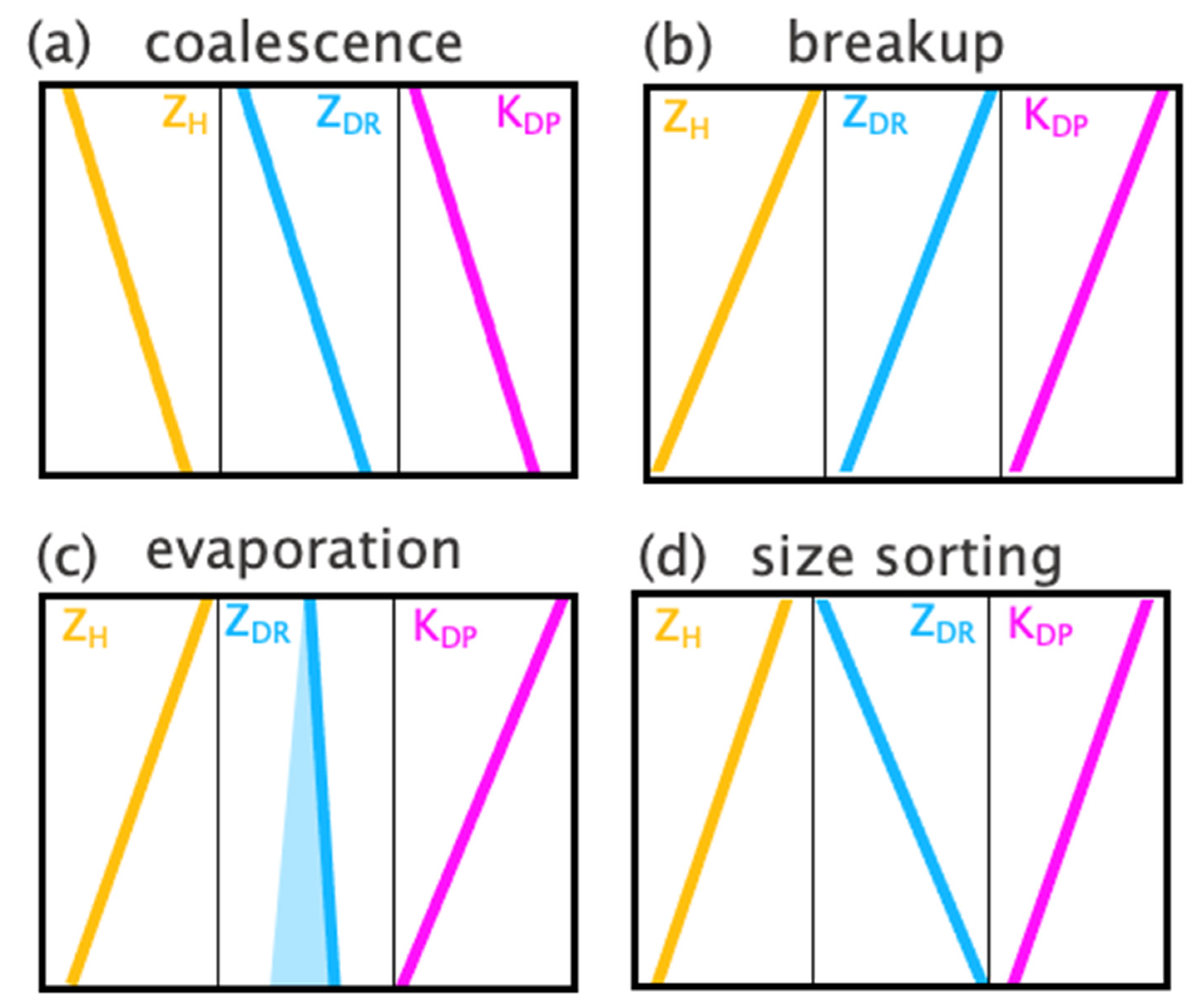
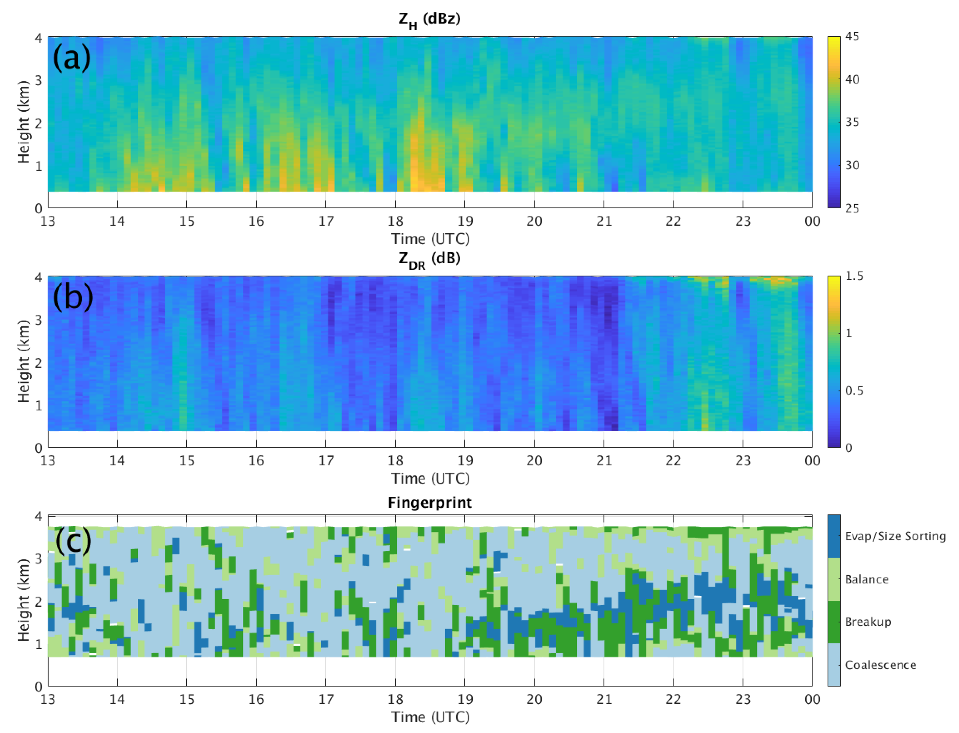
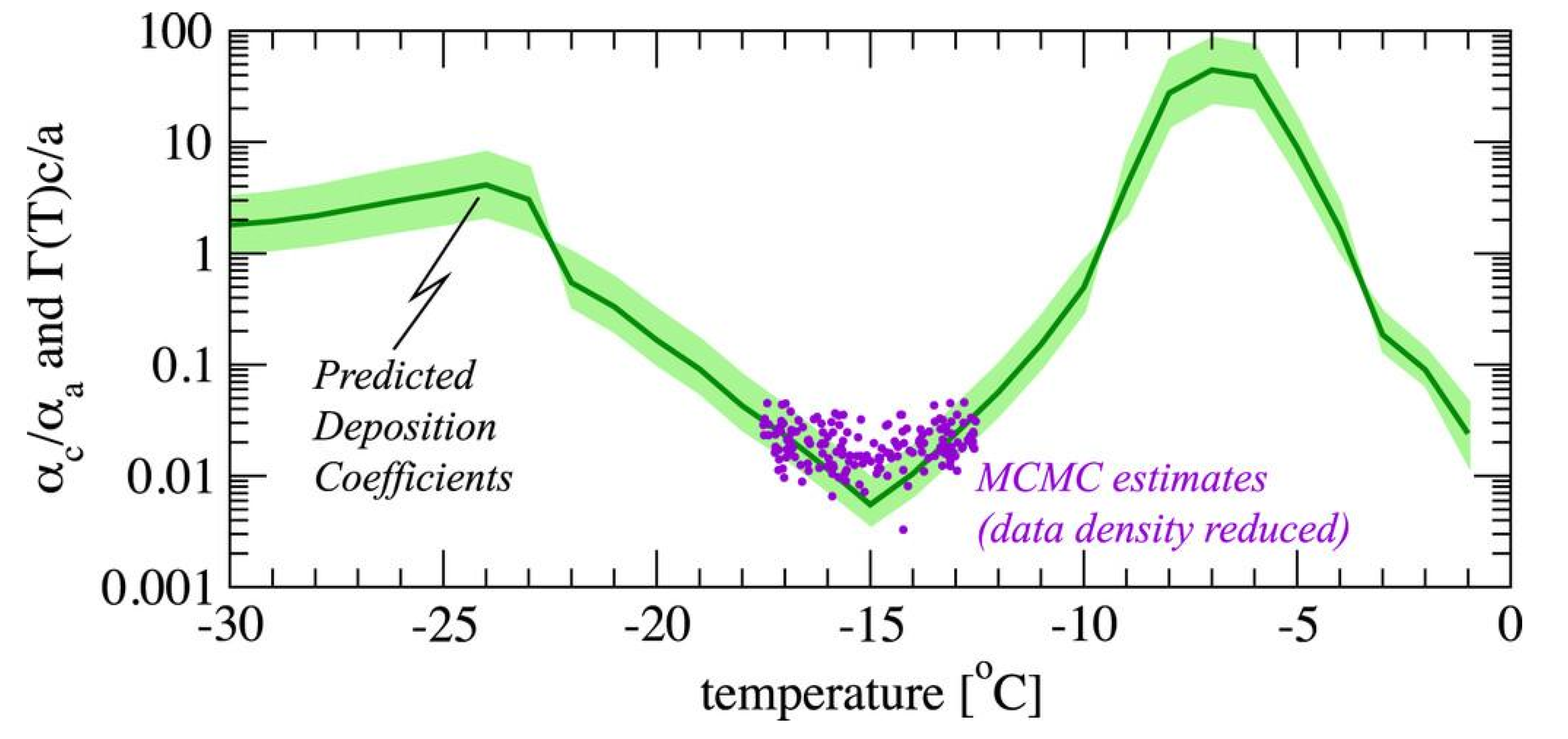
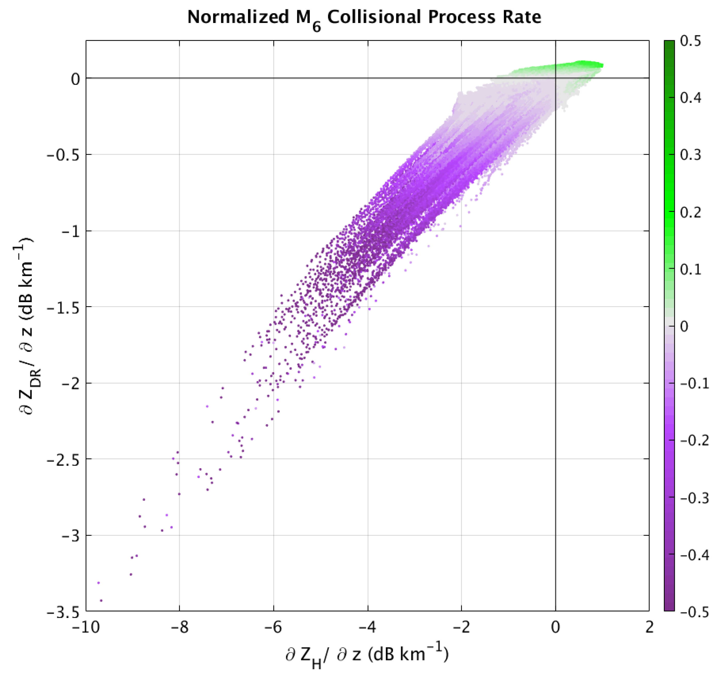
Table 1.
Summary of the changes in the polarimetric radar variables towards the ground for different microphysical processes. A positive sign + indicates an increase in that radar variable between the top and bottom of the profile, whereas a negative sign indicates a decrease. The presence of a second sign in brackets [] indicates the possible variation.
| Microphysical Processes | |||
|---|---|---|---|
| Collision-Coalescence | + | + | + |
| Breakup | |||
| Evaporation | − | ||
| Size Sorting | + | ||
| Vapor Deposition | + | + | + |
| Aggregation | + | ||
| Riming | + | ||
| Riming with ice splintering | + | + | |
| Sublimation | |||
| Sublimation with fragmentation | + | ||
| Refreezing | |||
| Melting * | + | + | + |
* The polarimetric radar signature of melting is accompanied by a sharp reduction in , which helps identify the process.
Publisher’s Note: MDPI stays neutral with regard to jurisdictional claims in published maps and institutional affiliations. |
© 2022 by the authors. Licensee MDPI, Basel, Switzerland. This article is an open access article distributed under the terms and conditions of the Creative Commons Attribution (CC BY) license (https://creativecommons.org/licenses/by/4.0/).
Share and Cite
MDPI and ACS Style
Kumjian, M.R.; Prat, O.P.; Reimel, K.J.; van Lier-Walqui, M.; Morrison, H.C. Dual-Polarization Radar Fingerprints of Precipitation Physics: A Review. Remote Sens. 2022, 14, 3706. https://0-doi-org.brum.beds.ac.uk/10.3390/rs14153706
AMA Style
Kumjian MR, Prat OP, Reimel KJ, van Lier-Walqui M, Morrison HC. Dual-Polarization Radar Fingerprints of Precipitation Physics: A Review. Remote Sensing. 2022; 14(15):3706. https://0-doi-org.brum.beds.ac.uk/10.3390/rs14153706
Chicago/Turabian StyleKumjian, Matthew R., Olivier P. Prat, Karly J. Reimel, Marcus van Lier-Walqui, and Hughbert C. Morrison. 2022. "Dual-Polarization Radar Fingerprints of Precipitation Physics: A Review" Remote Sensing 14, no. 15: 3706. https://0-doi-org.brum.beds.ac.uk/10.3390/rs14153706
Note that from the first issue of 2016, this journal uses article numbers instead of page numbers. See further details here.