Article

MBES Seabed Sediment Classification Based on a Decision Fusion Method Using Deep Learning Model

1
Acoustic Science and Technology Laboratory, Harbin Engineering University, Harbin 150001, China
2
Key Laboratory of Marine Information Acquisition and Security (Harbin Engineering University), Ministry of Industry and Information Technology, Harbin 150001, China
3
College of Underwater Acoustic Engineering, Harbin Engineering University, Harbin 150001, China
4
College of Geodesy and Geomatics, Shandong University of Science and Technology, Qingdao 266590, China
5
College of Oceanography and Space Informatics, China University of Petroleum (East China), Qingdao 266580, China
*
Author to whom correspondence should be addressed.
Remote Sens. 2022, 14(15), 3708; https://0-doi-org.brum.beds.ac.uk/10.3390/rs14153708
Submission received: 28 May 2022 / Revised: 14 July 2022 / Accepted: 27 July 2022 / Published: 2 August 2022

Abstract

:
High-precision habitat mapping can contribute to the identification and quantification of the human footprint on the seafloor. As a representative of seafloor habitats, seabed sediment classification is crucial for marine geological research, marine environment monitoring, marine engineering construction, and seabed biotic and abiotic resource assessment. Multibeam echo-sounding systems (MBES) have become the most popular tool in terms of acoustic equipment for seabed sediment classification. However, sonar images tend to consist of obvious noise and stripe interference. Furthermore, the low efficiency and high cost of seafloor field sampling leads to limited field samples. The factors above restrict high accuracy classification by a single classifier. To further investigate the classification techniques for seabed sediments, we developed a decision fusion algorithm based on voting strategies and fuzzy membership rules to integrate the merits of deep learning and shallow learning methods. First, in order to overcome the influence of obvious noise and the lack of training samples, we employed an effective deep learning framework, namely random patches network (RPNet), for classification. Then, to alleviate the over-smoothness and misclassifications of RPNet, the misclassified pixels with a lower fuzzy membership degree were rectified by other shallow learning classifiers, using the proposed decision fusion algorithm. The effectiveness of the proposed method was tested in two areas of Europe. The results show that RPNet outperforms other traditional classification methods, and the decision fusion framework further improves the accuracy compared with the results of a single classifier. Our experiments predict a promising prospect for efficiently mapping seafloor habitats through deep learning and multi-classifier combinations, even with few field samples.

Graphical Abstract

1. Introduction

Ocean ecosystems provide a wide range of services to humans, including food, resources, culture, climate control and provision of habitats. In recent years, as the demand for ocean space and resources has gradually expanded, large-scale human activities have put this system under enormous pressure [1,2]. Seafloor maps can provide essential information for ocean monitoring and management, mainly including seafloor topographic and seafloor habitat information. Seafloor habitats are referred as a “spatially defined area where the physical, chemical and biological environment is distinctly different from the surrounding environment” [3]. High-precision habitat mapping can contribute to the identification and quantification of the human footprint on the seafloor, by providing data for investigating the physical characteristics, spatial distribution, and ecological functions of biological communities and seafloor habitats. As a representative of seafloor habitat mapping, the classification of seafloor sediments has gradually drawn the interest of relevant scholars. Seabed sediments mainly refer to the constituents of the seafloor surface, consisting of the seafloor rocks and the surface sediments deposited during hydrodynamic action [4,5]. High-quality and full-coverage investigation of the seafloor sediments can help promote the application of marine scientific research, resource development, engineering construction, environmental protection, and military security in many fields [6,7]. At present, the exploration methods applied to the seabed sediments mainly include direct seafloor field sampling and indirect optical and acoustic methods [8]. Seafloor field sampling has the disadvantages of low efficiency and high cost, making it difficult to achieve a large-scale rapid survey. Optical remote sensing is also applied to seabed sediment mapping. However, because of the obvious attenuation of light in water, it can only be carried out in shallow water inshore with good water quality [9]. In contrast, acoustic waves have good water propagation properties and have been widely used for seabed sediment exploration and seafloor topography measurements [10,11].
With the rapid development of sonar systems and signal processing technologies, acoustic methods have shown great potential in seafloor habitat mapping. Researchers have used many devices, such as a multibeam, side-scan sonar, and sub-bottom profiler, to provide rich observational information for accurate exploration of seabed environments and seafloor geological structures [12,13]. When the frequency and angle of incidence are constant, the backscatter intensity depends on the seabed properties [14], which are closely related to the sediment types. A multibeam echo-sounding system (MBES), which can simultaneously acquire high-precision backscatter intensity information and corresponding seafloor topographic information, is one of the primary devices applied to acoustic seabed sediment classification studies currently [15,16].
To date, seabed sediment classification based on the MBES data is considered to be an important method to characterize the seafloor habitats [17,18,19]. The classification methods utilized in seabed sediment evaluation mainly focus on supervised and unsupervised classification. Among them, supervised classification methods mainly include K-nearest neighbor (KNN) [20], support vector machine (SVM) [21], decision tree (DT) [22], random forest (RF) [23], and back propagation neural network (BPNN) [24,25]. Unsupervised classification methods mainly include K-means clustering [26,27] and self-organizing feature map (SOM) neural networks [24]. However, sonar images have low contrast, high noise, obvious stripes and are susceptible to environmental conditions. The aforementioned classifiers mainly rely on the so-called “shallow structure” and cannot fully learn complex nonlinear features, posing a dilemma in terms of improving seabed sediment classification accuracy.
Recent researches have shown that deep learning can produce highly representative features through hierarchical learning, an advantage that s apparent when dealing with more complex data relationships [28]. Deep learning has better generalization ability and compatibility with the noise of images. Several recent studies have demonstrated the effectiveness of deep learning methods for seabed sediment classification, even if the MBES images have stripes and noises [9,29]. However, owing to the complex field conditions and high costs, the seabed sediment samples obtained from field sampling are very limited. To our knowledge, the existing deep learning networks usually require a large quantity of training samples because of the many parameters that need to be determined [30,31], which was hardly considered in previous MBES seabed mapping studies. In 2018, a new deep learning method named random patches network (RPNet) was proposed [32] and had been proven to be the most effective in hyperspectral image (HSI) classification, compared to the many existing deep learning methods. RPNet utilizes random projection for dimensionality reduction, which is beneficial for insufficient samples in the training process of the classifier [33]. RPNet combines both shallow and deep features, thus facilitating the extraction of sediment features with lower noise and more reliable information, while most deep learning methods only utilize the deepest feature [30,31,34]. Therefore, the RPNet may yield a good performance in seabed sediment mapping when the samples are limited.
However, RPNet also demonstrates some deficiencies when the sediments are mixed. The sediments are always small scale, with adjacent pixels often representing different substrate types, especially in mixed sediments. Similar to the classical convolutional neural networks, RPNet tends to have an over-smoothing phenomenon on small-scale sediments, which may falsely erase small useful features and cause misclassification. Furthermore, for seabed sediment acoustic classification, there is no strong statistical relationship between most features extracted from sonar images and sediment classes [35], which restricts the ability to extract useful information by a single classifier. In fact, different classifiers offer different generalization abilities in sample learning. The decision fusion algorithm based on voting strategies and fuzzy membership rules can inherit the advantages of every single classifier and take advantage of the complementarity between various classifiers through different fusion strategies. Thus, the misclassified pixels derived from RPNet with a lower fuzzy membership degree can be rectified by other shallow learning classifiers using the proposed decision fusion algorithm, which further improves the classification accuracy [28,36]. Previous studies have verified the effectiveness of the decision fusion method in remote sensing image classification [28,37], but it has not yet been introduced into the seabed sediment classification of acoustic images.
In this paper, we mainly consider the following questions:
(1)
The limited field samples and inevitable noise in acoustic images are obstacles for high accuracy seabed sediment classification. Can we find a classification framework that has good performance with small samples?
(2)
Although deep learning has been proved to be effective for seabed sediment classification, it may falsely erase small useful features and cause misclassification. In fact, any classifier, regardless of the architecture, has limited abilities to mine effective features and uncertainties in its predictions. Can we design an architecture to take advantage of the complementarity between deep and shallow learning classifiers?
In summary, the main contributions of this research article are as follows:
(1)
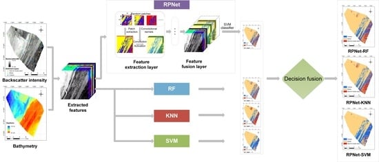
After feature extraction, we employ the RPNet algorithm for seabed sediment classification, which only needs a small number of samples during the training stage. The results are compared with several traditional machine learning methods (random forest, K-nearest neighbor, support vector machine and deep belief network) to verify the efficiency and effectiveness of RPNet. This algorithm may be a promising way to reduce the impact of few samples and noise on classification accuracy.
(2)
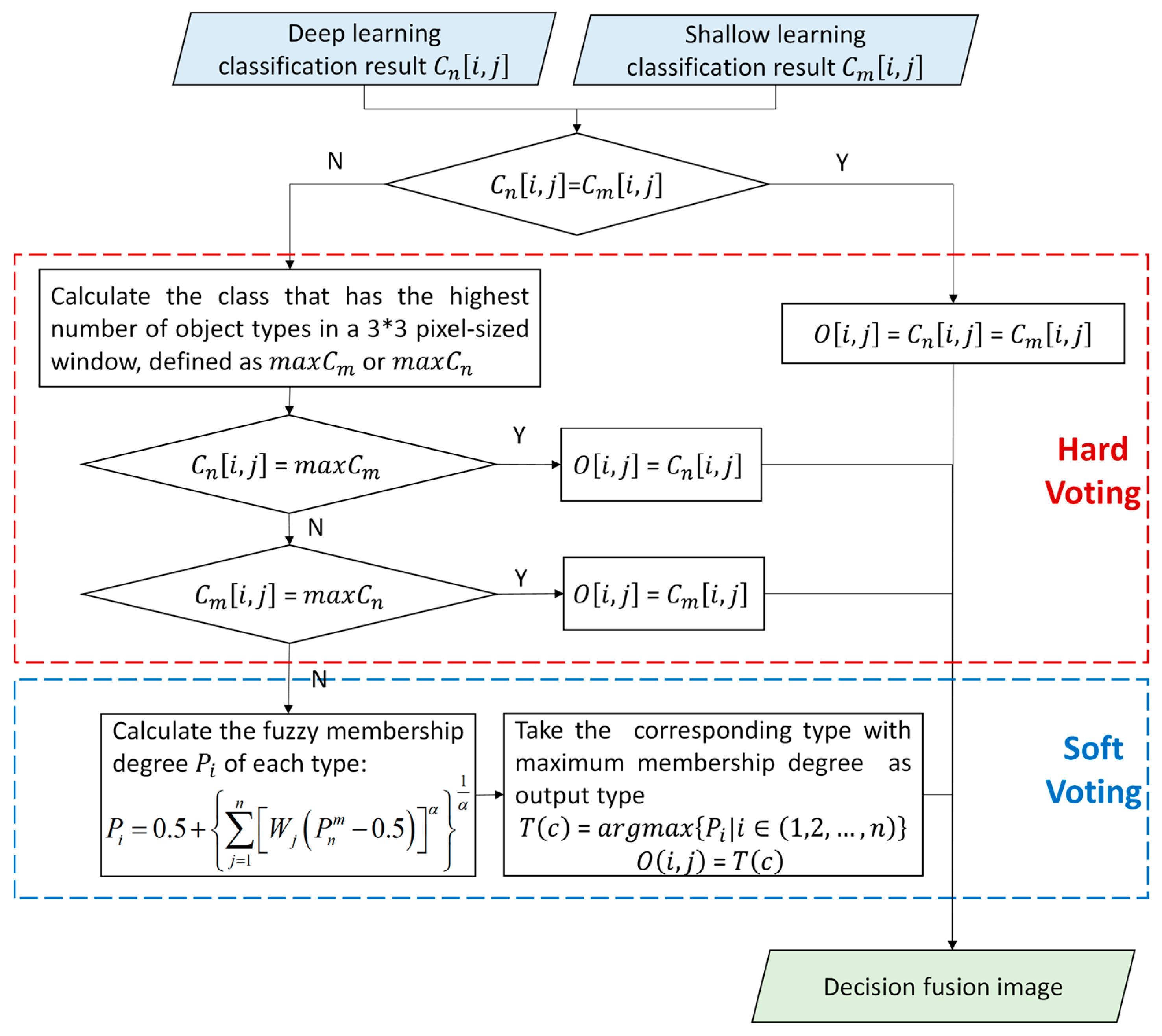
In order to take advantage of the complementarity between RPNet and other shallow architectures to alleviate the problem of over-smoothness and misclassification, we propose a deep and shallow learning decision fusion model based on voting strategies and fuzzy membership rules, which combines the seabed sediment classification results of RPNet and several traditional shallow learning classifiers. Then, a benchmark comparison is provided by the single classifier to evaluate the performance of our proposed decision fusion strategy.

2. Study Sites and Experimental Data

2.1. Study Sites

Two study sites, S1 and S2, were selected to investigate the validity and universality of the proposed method, both of which are in the sea around the United Kingdom. S1 is located in the southern North Sea. The North Sea is located in the northwestern part of the European continent and has a temperate maritime climate, whose average water depth is 91 m. According to JNCC [38], the southern North Sea has a mix of sediments, mainly covered by sandbanks and gravel beds. This site covers an area of approximately 44 km2, with a depth of 19–51 m, and gradually shows a deepening trend from northwest to southeast (Figure 1). S2 is situated in the southern Irish Sea, covering an area of 33,000 km2 [39]. Under the influence of high tidal activity and energy exchange intensity, the physical conditions and biological communities have varied significantly over these years, ranging from rocky reefs to deep mud basins [40]. Our research area is near Mid St George’s Channel, covering approximately 188 km2, and from west to east, the water depth gradually increases from 64 m to 124 m. S1 is next to the Straits of Dover and belongs to the Southern North Sea Marine Protected Areas (MPA); S2 covers the area of the Habitat Mapping for Conservation and Management of the Southern Irish Sea (HABMAP) surveys [40]. A growing number of institutions and scholars have conducted scientific research programs in these areas, aimed at understanding seafloor habitats and seafloor geology and providing support for benthic ecosystem conservation, the assessment of biotic and abiotic seafloor resources, and sustainable ocean development [40,41,42,43,44]. Hence, both of these two study sites make sense for seabed mapping and marine surveys.

2.2. Experimental Data

The experimental datasets contain the backscatter intensity data, bathymetry data, and ground-truth sediment samples. The samples were acquired via Hamon Grab. Multibeam backscatter and sample data are available from the British Geological Survey (BGS) GeoIndex Offshore [45], and the related bathymetry data are found in the Admiralty Marine Data Portal (UK Hydrographic Office). In S1, both the backscatter and bathymetry data are collected by Simrad/Kongsberg EM2040, using a frequency of 400 kHz. The manufacturer is Kongsberg Maritime in Kongsberg, Norway. The multibeam survey collected backscatter data from February to March 2012, and the bathymetry data were collected in January 2014 and processed by Caris HIPS. In S2, multibeam backscatter data and bathymetry data were gathered in March 2012 by Reson Seabat 7125, using a frequency of 200 kHz. The manufacturer is Teledyne Reson in Slangerup, Denmark. All the backscatter data were then resampled to 4 m.
Many practitioners used a simplified classification of the Folk triangle. This classification standard emerged at the request of UKSeaMap, i.e., a digital product more focused on the hierarchical European Nature Information System (EUNIS) habitat classification system [46]. Compared with the Folk triangle [47], the particle size criterion is changed to cover a larger area and finally includes the following four classes: sand and muddy sand, mud and sandy mud, mixed sediments, and coarse sediments (Figure 2). The mixed sediments correspond to mG, msG, gM, and gmS in Folk’s system, and coarse sediments correspond to G, sG and gS. In our experiment, the samples are divided into the following three classes: sand and muddy sand, mixed sediments, and coarse sediments.
Prior information on training samples was often matched manually based on ground data obtained directly from in-situ sampling techniques (underwater grabs, photos or videos, etc.) [9,48]. However, different positioning systems are utilized in the multibeam mapping technology and in-situ sampling, which may cause position deviation between the two data [49,50]. Therefore, we regard the 6 × 6 window centered on each sample as one type (same as the center type), and then select 25 groups of sediment samples with the highest Jeffries–Matsushita (J–M) separating degree. The J–M separating degree is a spectral separability index based on conditional probability theory. It is widely employed to evaluate the separability of different samples [51]. A higher separating degree is usually beneficial for classifying the different sediment types. We finally obtain 900 and 1440 samples in S1 and S2, and randomly select training and test samples according to the ratio of 7:3 (Table 1).

3. Methods

A novel deep and shallow learning decision fusion model is proposed for the classification of seabed sediments. The method consists of the following steps. (1) Since both the backscatter and bathymetry information reflect the distribution of seabed sediments, we extract some features from the backscatter and bathymetry data as the input of the classifiers. (2) To overcome the influence of obvious noise and the lack of training samples, we build an RPNet model and compare it with traditional methods. (3) In order to alleviate the over-smoothing phenomenon and misclassifications of RPNet, we propose a decision fusion framework based on voting strategies and fuzzy membership rules, which combines RPNet and traditional methods, and obtains the final classification maps.
The principles and major workflows are detailed hereafter.

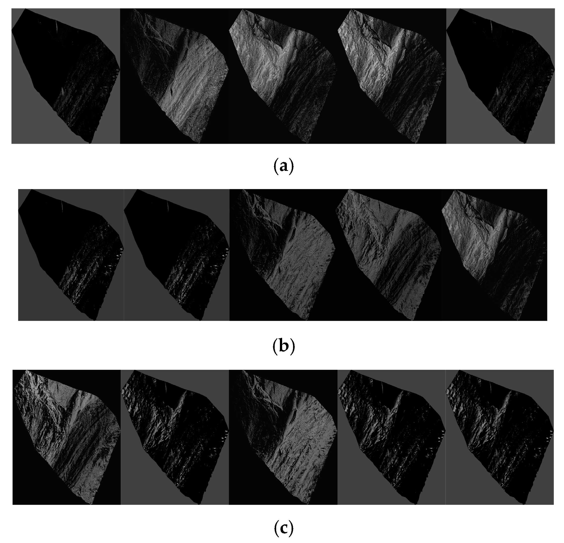
3.1. Feature Extraction

In order to construct a stable mapping relationship between the raw acoustic data and the actual sediment type, feature extraction is the foundation for correct sediment identification. To date, the multibeam backscatter intensity feature is the most widely used feature in habitat mapping studies [35,52,53]. In addition, bathymetry and bathymetry-derived variables are the most intuitive representation of seafloor topography. All of the topographic features are derived from bathymetry, including aspect, slope, curvature, bathymetric position index (BPI), roughness, etc. Since the distribution of different seabed sediment types has a high correlation with the topography of the seafloor, it is demonstrated that the combination of backscatter intensity features and topographic features plays a more effective role in the seabed sediment classification [53,54]. By removing the features with much noise and low separability between different classes, we finally choose 8 and 9 features for S1 and S2 (Table 2) as the input features.

3.2. RPNet Framework

In this section, we present a deep learning method, namely, RPNet. The RPNet is based on the theory of random projection, which is exploited to achieve classification by projecting data into a random low dimensional space. In random projection, the original d-dimensional data X N × d are projected to a k-dimensional subspace through the origin, using a random matrix R d × k [32].
X R P = X R N × k
Relevant researches have demonstrated that in low-dimensional space, only a small number of samples are required in the training process. By regarding the random patches as convolutional patches and feature fusion of different layers, the RPNet combines both shallow and deep features, so as to obtain more useful features and obtain higher classification accuracy. As shown in Figure 3, the RPNet consists of an input layer, several feature extraction layers, a feature fusion layer, an SVM classifier, and an output layer.

3.2.1. Input Layer

For the input image, r, c, n are the number of rows, columns, and bands, respectively. Since the data ranges of each input layer are quite different, the first step is data normalization, and the data are scaled in the range of (−1, 1). Then, principal component analysis (PCA) is applied to project the high-dimension data to a lower dimension and reserve the first p PCs so that the redundancy between different bands is reduced. In order to decrease the correlation and obtain a similar variance between different bands, the whitening operation is utilized [59].

3.2.2. Feature Extraction Layer

The feature extraction layer first extracts k  w × w × p -sized random patches as convolution kernels. After convolving the whitening features, these k features are activated by the rectified linear unit (ReLU) function. The moving stride is set as 1. Traditional convolutional kernels are set manually at the beginning of the deep learning methods, whereas RPNet extracts random patches from whitening features as kernels. There are complete L feature extraction layers in the whole RPNet structure.
The formula below denotes the feature map I i calculated by the ith random patch.
I i = f ( j = 1 p X ( j ) ( P i ( j ) × i ) ) ,   i = 1 , 2 , , k ,
where I i denotes the ith feature map and X ( j ) is the j th dimension of the data after PCA and whitening. is the convolution operator, P i ( j ) means the jth dimension of the i th random patch, and i is the weight of the i th random patch. f (   ) represents the rectified linear unit activation function.
f ( x ) = { x ,   x > 0 0 ,   x 0 f ( x ) = max ( 0 , x )
The feature maps of the l th layer are shown by the following equation:
I ( l ) = f ( j = 1 p i = 1 k X ( j ) ( P i ( j ) × i ) ) ,   l = 1 , 2 , , L

3.2.3. Feature Fusion Layer and SVM Classifier

After a series of feature extraction operations, the features from each feature extraction layer I ( l ) and the original image In form the final classification data I . By stacking layers of every feature extraction result, both shallow and deep features are utilized, including multi-scale information of different objects. The stacking layer can be represented as follows:
I = { I ( 1 ) , I ( 2 ) , , I ( L ) , I n }
To increase the convergence efficiency, each dimension S of I is normalized to be i s ˜ , which is as follows:
i s ˜ = i s mean ( i s ) var ( i s ) ,   s = 1 , 2 ,   , l k + n ,
where i s denotes the Sth dimension of I and mean ( i s ) and var ( i s ) denote the mean and variance value of i s , respectively.
Finally, all the features are inputted into the SVM (with RBF kernels) classifier. SVM can improve the performance in terms of training speed and classification accuracy.
The convolution operation contributes to a bigger receptive field. As the layer becomes deeper, the receptive field in the RPNet will become larger. Generally, with the fixed kernel size, the relationship between the receptive fields RF and the number of layers l is as follows:
R F = l × ( w 1 ) + 1 ,
where (w − 1) represents the RF increment for every convolution operation.

3.3. Decision Fusion Method Based on Multi Classifiers

RPNet tends to have an over-smoothing phenomenon on small-scale sediments, which may falsely erase small useful features and cause misclassification. In fact, any classifier, regardless of the architecture, has limited abilities to mine effective features and uncertainties in its predictions. Therefore, we propose a decision fusion method based on the voting strategy and fuzzy membership to rectify the misclassifications of RPNet by other shallow learning methods. Traditional voting methods include hard voting and soft voting. The former directly outputs class labels and the latter outputs class probabilities. Hard voting selects the class with the largest number by different classifiers, while soft voting calculates the weighted average of the class probabilities of each class and selects the class with the highest value. Our proposed decision fusion method combines the hard voting and soft voting strategy (Figure 4). Hard voting is first utilized to carry out preliminary classification, and then the fuzzy membership algorithm as soft voting is introduced to estimate the unknown types. Using the proposed decision fusion algorithm, the misclassified pixels with a lower fuzzy membership degree can be rectified by other classifiers. The flowchart of deep and shallow learning decision fusion is shown as follows.
In this framework, the deep and shallow learning classification results C n [ i , j ] and C m [ i , j ] are combined as the input. In this experiment, RPNet is used as the deep architecture; RF, KNN and SVM are chosen as the shallow structure. The final type O [ i , j ] in the [ i , j ] location is calculated pixel by pixel. After the hard voting method is applied for some pixels, other pixels are decided by the fuzzy membership degree.
P i = 0.5 + { j = 1 n [ W j ( P n m 0.5 ) ] α } 1 α ,
where P i is the membership degree of type n . W j denotes the weight of each classifier, which depends primarily on the classification accuracy. In our experiments, if one supposes that the classification accuracy of the two classifiers is a and b, respectively, W 1 = a / ( a + b ) , W 2 = b / ( a + b ) , P n m is the membership degree of C m [ i , j ] , belonging to the type n. One must note that j = 1 n W j = 1 and α is an odd number. In this experiment, we set α as 3, mainly based on past experience [37] and the principle of reducing computational expense. In the end, the type with the maximum membership degree is set as the best result.

4. Experiments and Results

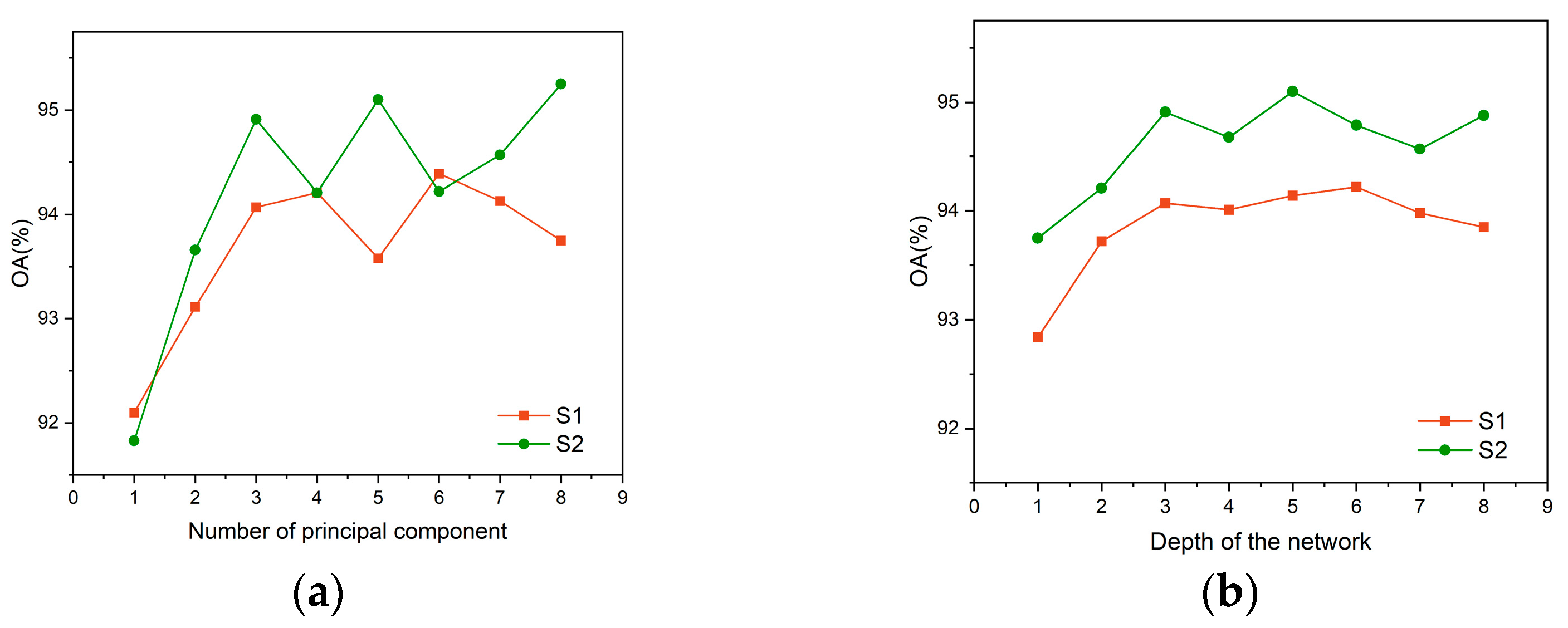
4.1. Parameter Setting of RPNet

In the experiments, the optimal parameters of classifiers were adjusted by five-fold cross-validation. Generally speaking, as the number of pc layers p and feature extraction layers L increases from 3, the computational expense increases, with no obvious promotion in classification accuracy [32]. We evaluate the classification accuracies of different p and L. Figure 5 shows that as p and L grows, the accuracies of both datasets have a trend of rising first; after the number reaches 3, the accuracies fluctuate around 94%. Therefore, we set p and L as 3. Although the size of kernels w usually is beneficial for the classification task, too large w also leads to the over-smoothing phenomenon because of the small scale of the sediments. Thus, we set the parameter w as 5. As for the number of patches k, the RPNet becomes more time-consuming as k grows (Figure 6), so we initially set k to be less than 20. In S1, when k is 5 or 10, the overall accuracy (OA) is relatively high. In S2, classification with 5 or 20 random patches is highly accurate. We finally set k as 5 as a tradeoff between time cost and accuracy for both datasets.
To better understand what RPNet learns in the different layers, the feature extraction results of each layer are displayed in Figure 7 and Figure 8. From these figures, we can find that the first layer has more obvious distribution characteristics, while in deeper layers, the extracted features tend to be more abstract and have fewer details.
The experiments were implemented on a computer equipped with an Intel i7-8700 3.20-GHz processor with 16 GB of RAM and an Intel (R) UHD Graphics 630 graphic card.

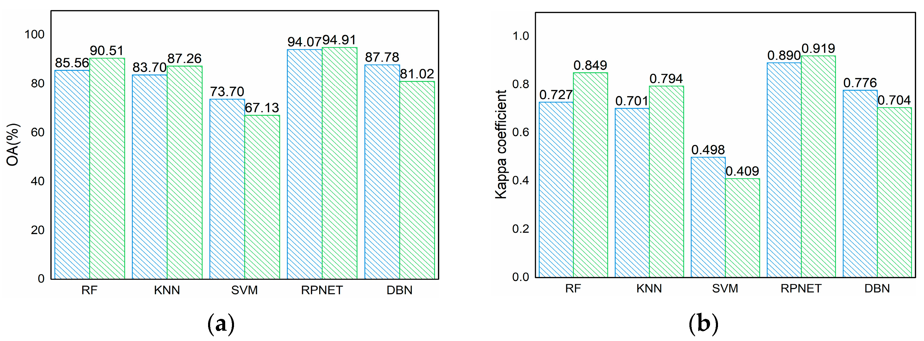
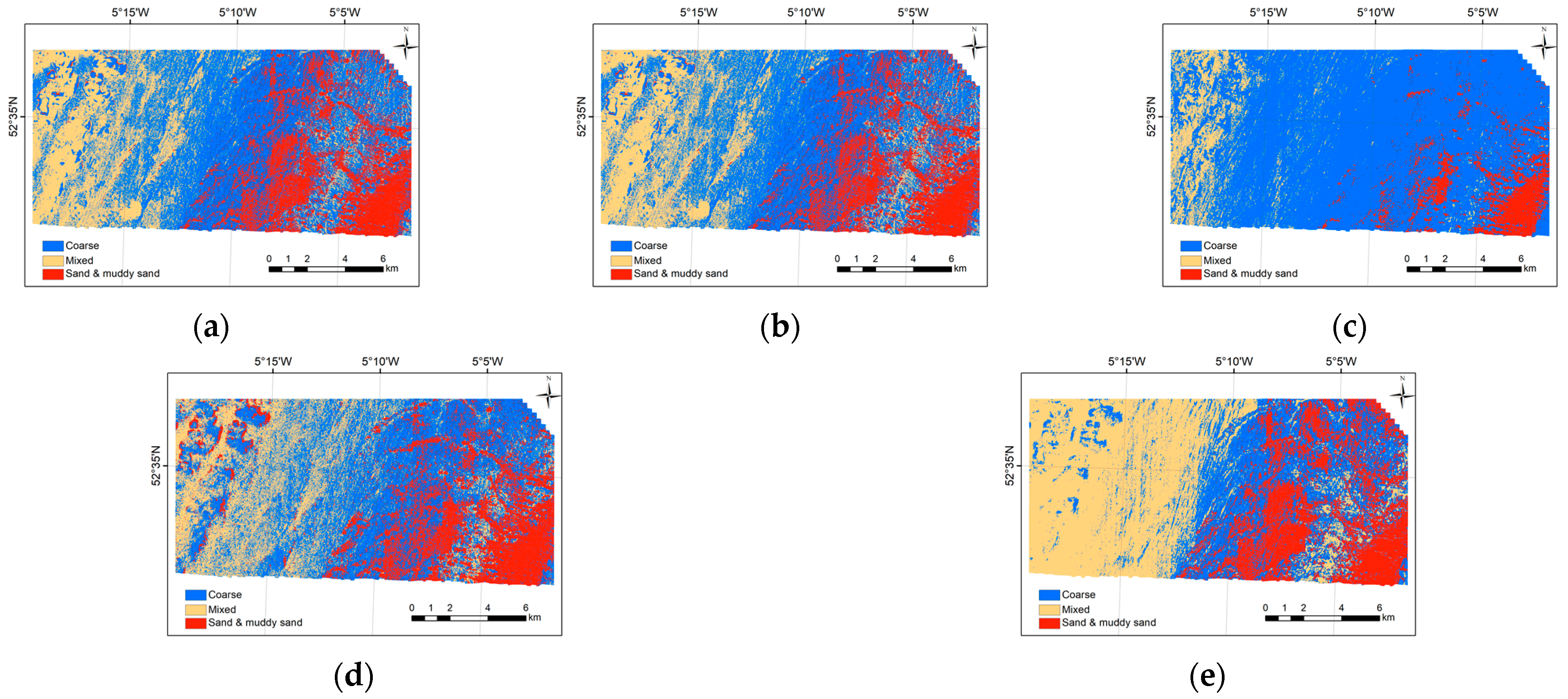
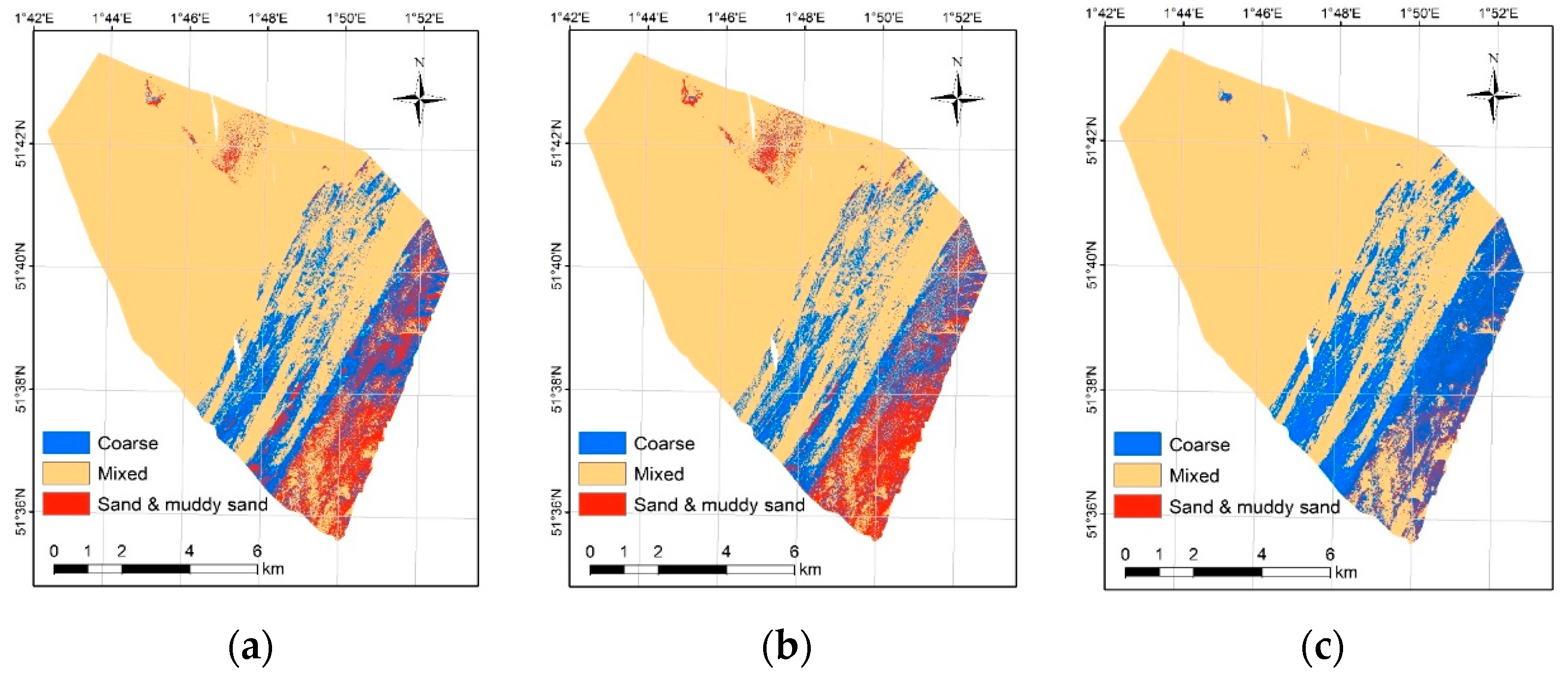
4.2. Classification Results of RPNet

Based on the backscatter and topographic features, we constructed an RPNet model to classify the sediment types in the research field. In the experiments, the values of user’s accuracy (UA), producer’s accuracy (PA), overall accuracy, and Kappa coefficient [60,61] were adopted as evaluation indicators.
P A = x i i x i +
U A = x i i x + i
O A = i = 1 n x i i S
K a p p a   c o e f f i c i e n t = S i = 1 n x i i i = 1 n ( x + i x i + ) S 2 i = 1 n ( x + i x i + )
where n is the number of sediment types, x i i denotes the number of diagonals along the confusion matrix, x + i denotes the statistical results of different classes by prediction, and x i + indicates the statistics of different classes of ground truth samples. S is the number of all the samples.
Due to the unbalanced seabed sediment samples, we also introduced the F1 score to demonstrate the classification capacities of classifiers. F1 score represents a weighted average of precision and recall, thus is commonly used as a reliable evaluation indicator for the classification of unbalanced datasets [62].
F 1   s c o r e = 2 × ( p r e c i s i o n × r e c a l l ) ( p r e c i s i o n + r e c a l l )   ,
where p r e c i s i o n = t p / ( t p + f p ) , r e c a l l = t p / ( t p + f n ) , t p is the number of true positives, f p is the number of false positives and f n is the number of false negatives.
From Table 3 and Table 4, it can be observed that in S1, the mixed sediments obtain the highest accuracy (over 96%); whilst although the coarse sediments have the lowest accuracy, it still reaches around 88%. In S2, sand and muddy sand exhibit the highest accuracy (over 98%), whereas the accuracy of mixed sediments with the smallest number is lower than the other classes. In order to further verify the effectiveness of the RPNet, the RPNet results are reported along with three shallow learning classification methods, including RF, KNN, and SVM. RPNet is also compared with the deep belief network (DBN), which is a typical deep learning algorithm utilized in seabed sediment classification recently [9].
Figure 9 shows the results of seabed sediment classification performed by the aforementioned classifiers. As shown in Figure 9, RPNet consistently reports the best classification OA, with up to 94.07% for S1 and 94.91% for S2, higher than that of RF (85.56% and 90.51%, respectively), KNN (83.70% and 87.26%, respectively), SVM (73.70% and 67.13%, respectively), and DBN (87.78 and 81.02%, respectively). Moreover, the F1 score also demonstrates that a significant increase has been achieved by RPNet over the RF, KNN, SVM, and DBN, with F1 scores of 0.854, 0.840, 0.712 and 0.877 for S1 and F1 scores of 0.905, 0.872, 0.635 and 0.810 for S2, respectively. As for time expense, although the operating time of KNN is significantly less than the other classifiers, the accuracy of KNN is remarkably lower (10.37% for S1 and 7.65% for S2) than that of RPNet. With an accuracy of over 85%, the RF method is very time-consuming. DBN outperforms other classifiers in S1, but has a lower performance than RF, KNN and RPNet in S2, which may indicate poorer robustness and universality than RPNet. As a tradeoff between accuracy and time, the most appropriate method is RPNet.
The accuracy of each sediment type was also summarized (Figure 10). It can be illustrated that their classification accuracies are ordered as follows: SVM < KNN < RF < RPNet. RPNet outperforms other classifiers for almost all the classes at both study sites in terms of accuracy. For RF, the largest increase is up to 26.83% and 5.13% for the class of sand and muddy sand in S1 and S2. Similarly, for KNN, the greatest increase in accuracy is up to 22.31% for the class of sand and muddy sand in S1 and S2. For the class of mixed sediments and coarse sediments, the accuracy of the RPNet is also larger than that of the RF, up to 5.29% and 4.76% for S1 and S2. SVM fails to perform well, whose accuracy of sand and muddy sand is only 12.2% in S1 and 41.88% in S2. The accuracies of the other sediments are slightly lower than that of KNN.
These classification methods were also visually evaluated to obtain the sediment maps (Figure 11 and Figure 12). From northwest to southeast, mixed sediments, coarse sediments, and sand and muddy sand are mainly distributed along these areas. Except for SVM, these different classification maps generally have consistent distributing patterns. The results of RPNet seem to consist of fewer omission and commission errors, which reflects the impressive capability and stability of the classifier. However, some undesirable noises in the RPNet results still remain, such as some misclassifications in detail and over-smoothness to some degree.

4.3. Decision Fusion Results

Based on the seabed sediment classification results of RPNet and several shallow learning classifiers (RF, KNN, and SVM), a deep and shallow learning decision fusion framework was then proposed. With this method, the misclassified pixels in RPNet with a lower fuzzy membership degree can be rectified by other shallow learning classifiers. As we can observe from Table 5 and Table 6, the RPNet-RF has the best performance, which enables an increase in accuracy compared with RPNet (up to 2.97% and 1.15% respectively). The greater improvement occurs in study site 1, where the accuracies of all of the three classes are over 2.4% larger than the RPNet. All of the decision fusion methods have noticeable improvements compared with the shallow learning methods. RPNet-KNN reveals the most significant increase of 11.86% and 6.72%, followed by RPNet-RF with 11.48% and 5.55% for S1 and S2. RPNet-SVM has minimal improvement, with up to 6.67% for S1 and 1.16% for S2. In S1, RPNet-RF and RPNet-KNN have a similar pattern, where sand and muddy sand exhibit the highest increase of 31.71% (in S1) and 24.75% (in S2), respectively; mixed sediments and coarse sediments have a 7–10% increase compared with the single classifier. However, for RPNet-SVM, the classes with low accuracy only show a slight increase or remain steady in terms of classification accuracy over SVM, which may be attributed to the too poor classification of sand and muddy sand. It can be estimated that decision fusion is sensitive to the poor classification performance of the input and cannot effectively obtain the desired results in this case.
The result maps after decision fusion show a similar distribution pattern with RPNet (Figure 13 and Figure 14). However, the RPNet-RF appears to remove undesirable noises and alleviate the over-smoothing phenomenon, especially in mixed areas with various classes. In S1, compared with the RPNet result, a small area in the north with sand and muddy sand has a noticeable change, with an area reduction in sand and muddy sand and more coarse sediments scattering within the area. In short, the RPNet with deep architecture and the classifiers with a shallow structure can provide complementary information, resulting in the rectification of the losses and errors in detail and better classification performance than any classifier alone.

5. Discussion

In this research, a deep and shallow learning decision fusion method was proposed for seabed sediment classification based on MBES backscatter and topographic data. This method inherits the advantages of deep and shallow learning classifiers and obtains a desirable classification result.
The results show that the RPNet method consistently reports the best classification accuracy and has good robustness against noise data. The performance of RPNet is better than that of RF and SVM, especially for SVM (with an accuracy of about 70%). However, in previous comparative studies for seabed mapping, SVM and RF tended to show good performance [21]. Cui et al. implemented an SVM classification method based on an Askey–Wilson polynomial kernel function in New Zealand and obtained an accuracy of 90.02% [50], but the universality still needs further validation because the study area was small. RF has become increasingly popular in recent years [18,22,52,53]. Diesing et al. compared the classification results of several classical models and performed model ensembling with an accuracy of only 84% [53]. Ji et al. proposed a selecting optimal random forest (SORF) and compared the accuracy with SVM and RF in Jiaozhou Bay [18]; the results showed that SORF produced the highest accuracies (85.00%), followed by RF and SVM. However, the number of samples per class reached several thousand, so the practicality of the method when lacking field samples needs to be explored. Wang et al. established a two-stage model using the XGBoost algorithm and the grain size parameters, which outperformed other classifiers, while grain size parameters are needed in this method [63]. In the aforementioned studies, RF tends to achieve higher accuracy than SVM. Our proposed algorithm performs better than RF and SVM may be because these classifiers are sensitive to noises in sonar images and their shallow structures are unable to learn enough useful characteristics. As for DBN, such deep learning methods have been applied in sediment classification recently, but methods applicable to small samples have hardly been specifically considered [9].

5.1. Effect of Sample Size on Classification Performance

To further explore the influence of sample size on classification performance, we reduced the number of samples to test the performance stability of RPNet and compared it with other classifiers. As is shown in Figure 15 and Figure 16, for RF and KNN, fewer training samples lead to a noticeable decrease in accuracy in S1, especially for coarse sediments (from about 0.8 to 0.7). For S2, when the sample size decreases, the accuracies of KNN and RF show a decrease, up to 3.57% (OA) and 0.035 (F1 score). Similar patterns are found, meaning that the DBN algorithm with more training samples is more accurate in both of the two areas. For both of the two sites, the SVM classification results are not significantly related to sample size, whose precision remains at a low level. In contrast, when the number of training samples decreases, the classification accuracy of RPNet remains steady in S1 and shows a slight downtrend in S2. The reason may be that the RPNet uses random patches to form the random matrices in random projection, which is employed to project data to a lower dimension space [32,33]. This property provides the possibility for high precision classification when samples are limited. When train: test = 7:3, the PA of coarse sediments is 88.13% and 94.76%, while the PA is 92.31% and 91.06% when train: test = 5:5 in S1 and S2, respectively. The reason may be that when the number of training samples decreases, some of the training samples that are not beneficial to the classification are reduced in S1.
The proposed decision fusion method takes advantage of the merits of the two classifiers and overcomes their individual shortcomings, thus demonstrating better performance than any classifier alone. As can be observed from the Table 5 and Table 6, the classification accuracy of a single shallow learning classifier is low for classes that are relatively less abundant, while the decision fusion method can substantially improve the accuracy of these classes. This phenomenon indicates the potential for application in unbalanced datasets. However, for classes with less than 50% accuracy (e.g., sand and muddy sand in the results of SVM), the proposed framework appears to be ineffective. It can be estimated that decision fusion is sensitive to the poor classification performance of the input and cannot obtain the desired results in this case.

5.2. Distribution of Topographic Features for Different Sediment Types

Numerous studies have indicated that combining backscatter and topographic information is more effective for multiple habitats characterization than only using backscatter intensity information [64]. In order to intuitively show the influence of topographic factors on the sediment distribution, this paper uses boxplots for the statistics of sediment distribution in topographic features (taking S1 as an example). As is shown in Figure 17, these selected topographic features all show a noticeable distinction between different types, which means that these features may contribute to the classification task. For instance, sand and muddy sand and coarse sediments can be easily distinguished in the bathymetry, mean depth, and minimum curvature features. The distributing aspect of mixed sediments is relatively concentrated, mainly floating at 100–280 degrees. Moreover, mixed sediments are widely distributed throughout the study area, mainly concentrated in relatively shallow water areas. Sand and muddy sand and coarse sediments are primarily distributed at depths of 40–50 m. These results are generally consistent with the east-west partition of sediment types shown in the classification results. Whilst some studies have demonstrated the correlation between topographic factors and sediment types [22,65], more experiments and in-depth analyses are still needed to draw general patterns.

5.3. Other Considerations

To a certain extent, our decision fusion method proposes a novel idea for the classification of seabed sediment on the premise of a single machine learning algorithm. However, the MBES images utilized in this paper tend to have noticeable stripe effects, which may be due to inadequate image mosaic processing of multibeam backscatter images in the pre-processing procedure. Even though we used the median filter and feature selection and found a proper classifier to reduce the noise, some striping noise can still be found in the results. Unsuitable network parameters and inappropriate feature selection may also lead to the loss of details, so it is better to find a more efficient way to optimize the feature selection and the model parameter setting method. In the future, we will investigate more feasible data pre-processing methods to solve this problem from the originally acquired multibeam backscatter intensity data, and extend the proposed method in more areas. Furthermore, except for the fusion of different classifiers, multisource data fusion can be considered for seabed sediment classification.

6. Conclusions

In this paper, a deep and shallow learning decision fusion method was proposed for seabed sediment classification based on MBES backscatter and topographic data. First, by combining both backscatter and topographic features, a deep architecture suitable for small samples, namely RPNet, was employed for classification; the results of which are statistically more accurate than the other existing traditional classifiers (RF, KNN, SVM and DBN). Then, a decision fusion method was proposed based on deep and shallow learning classifiers, which helps to compensate for the loss and errors of details, as well as alleviate the over-smoothing phenomenon on small-scale sediments. The effectiveness of the algorithm was tested in two areas in Europe using MBES images. This algorithm acquires the OA of 97.04% for S1 and 96.06% for S2, and consistently outperforms all of the individual classifiers. Our method takes advantage of the merits of deep learning and shallow learning methods. This study provides the possibility of high-precision classification with few training samples, which indicates a broad prospect for detailed mapping of seabed habitats and has important implications for estimating the long-term effects of human activities on the seafloor. In the future, more feasible data pre-processing methods and appropriate model parameter setting strategies are needed to alleviate the stripe noises and misclassifications.

Author Contributions

Conceptualization, J.W. and Z.Q.; methodology, J.W.; software, Z.Q.; writing—original draft preparation, J.W.; writing—review and editing, X.C., F.Y. and M.Y.; supervision, B.M. and X.L.; funding acquisition, Z.Q., B.M. and X.L. All authors have read and agreed to the published version of the manuscript.

Funding

This research was funded by the National Natural Science Foundation of China, grant number 41876053, 42006064, 42106070.

Institutional Review Board Statement

Not applicable.

Informed Consent Statement

Not applicable.

Data Availability Statement

The related original data of this article are available from http://mapapps2.bgs.ac.uk/geoindex_offshore/home.html (accessed on 1 April 2022) and https://data.admiralty.co.uk/portal/apps/sites/#/marine-data-portal (accessed on 1 April 2022).

Acknowledgments

The authors want to thank the British Geological Survey (BGS) and UK Hydrographic Office for providing the multibeam dataset and ground-truth samples and thank the editors and reviewers for their valuable comments and suggestions to improve the manuscript.

Conflicts of Interest

The authors declare no conflict of interest.

References

  1. Halpern, B.S.; Frazier, M.; Potapenko, J.; Casey, K.S.; Koenig, K.; Longo, C.; Lowndes, J.S.; Rockwood, R.C.; Selig, E.R.; Selkoe, K.A.; et al. Spatial and temporal changes in cumulative human impacts on the world’s ocean. Nat. Commun. 2015, 6, 7615. [Google Scholar] [CrossRef] [PubMed] [Green Version]
  2. Madricardo, F.; Foglini, F.; Campiani, E.; Grande, V.; Catenacci, E.; Petrizzo, A.; Kruss, A.; Toso, C.; Trincardi, F. Assessing the human footprint on the sea-floor of coastal systems: The case of the Venice Lagoon, Italy. Sci. Rep. 2019, 9, 6615. [Google Scholar] [CrossRef] [PubMed]
  3. Kostylev, V.E.; Todd, B.J.; Fader, G.; Courtney, R.C.; Cameron, G.; Pickrill, R.A. Benthic habitat mapping on the Scotian Shelf based on multibeam bathymetry, surficial geology and sea floor photographs. Mar. Ecol. Prog. Ser. 2001, 219, 121–137. [Google Scholar] [CrossRef] [Green Version]
  4. Zhi, H.; Siwabessy, J.; Nichol, S.L.; Brooke, B.P. Predictive mapping of seabed substrata using high-resolution multibeam sonar data: A case study from a shelf with complex geomorphology. Mar. Geol. 2014, 357, 37–52. [Google Scholar] [CrossRef]
  5. Ward, S.L.; Neill, S.P.; Van Landeghem, K.J.J.; Scourse, J.D. Classifying seabed sediment type using simulated tidal-induced bed shear stress. Mar. Geol. 2015, 367, 94–104. [Google Scholar] [CrossRef] [Green Version]
  6. Diesing, M.; Mitchell, P.J.; O Keeffe, E.; Gavazzi, G.O.A.M.; Bas, T.L. Limitations of Predicting Substrate Classes on a Sedimentary Complex but Morphologically Simple Seabed. Remote Sens. 2020, 12, 3398. [Google Scholar] [CrossRef]
  7. Zelada Leon, A.; Huvenne, V.A.I.; Benoist, N.M.A.; Ferguson, M.; Bett, B.J.; Wynn, R.B. Assessing the Repeatability of Automated Seafloor Classification Algorithms, with Application in Marine Protected Area Monitoring. Remote Sens. 2020, 12, 1572. [Google Scholar] [CrossRef]
  8. Strong, J.A.; Clements, A.; Lillis, H.; Galparsoro, I.; Bildstein, T.; Pesch, R. A review of the influence of marine habitat classification schemes on mapping studies: Inherent assumptions, influence on end products, and suggestions for future developments. ICES J. Mar. Sci. 2019, 76, 10–22. [Google Scholar] [CrossRef] [Green Version]
  9. Cui, X.; Yang, F.; Wang, X.; Ai, B.; Luo, Y.; Ma, D. Deep learning model for seabed sediment classification based on fuzzy ranking feature optimization. Mar. Geol. 2021, 432, 106390. [Google Scholar] [CrossRef]
  10. Kruss, A.; Madricardo, F.; Sigovini, M.; Ferrarin, C.; Gavazzi, G.M. Assessment of submerged aquatic vegetation abundance using multibeam sonar in very shallow and dynamic environment. In Proceedings of the 2015 IEEE/OES Acoustics in Underwater Geosciences Symposium (RIO Acoustics), Rio de Janeiro, Brazil, 29–31 July 2015; pp. 1–7. [Google Scholar] [CrossRef]
  11. Khomsin; Mukhtasor; Pratomo, D.G.; Suntoyo. The Development of Seabed Sediment Mapping Methods: The Opportunity Application in the Coastal Waters. IOP Conf. Ser. Earth Environ. Sci. 2021, 731, 012039. [Google Scholar] [CrossRef]
  12. Manik, H.M.; Nishimori, Y.; Nishiyama, Y.; Hazama, T.; Kasai, A.; Firdaus, R.; Elson, L.; Yaodi, A. Developing signal processing of echo sounder for measuring acoustic backscatter. In Proceedings of the 3rd International Conference on Marine Science (ICMS), Bogor City, Indonesia, 4 September 2019. [Google Scholar] [CrossRef]
  13. Luo, X.; Qin, X.; Wu, Z.; Yang, F.; Wang, M.; Shang, J. Sediment Classification of Small-Size Seabed Acoustic Images Using Convolutional Neural Networks. IEEE Access 2019, 7, 98331–98339. [Google Scholar] [CrossRef]
  14. Snellen, M.; Gaida, T.C.; Koop, L.; Alevizos, E.; Simons, D.G. Performance of Multibeam Echosounder Backscatter-Based Classification for Monitoring Sediment Distributions Using Multitemporal Large-Scale Ocean Data Sets. IEEE J. Ocean. Eng. 2019, 44, 142–155. [Google Scholar] [CrossRef] [Green Version]
  15. Montereale Gavazzi, G.; Kapasakali, D.A.; Kerchof, F.; Deleu, S.; Degraer, S.; Van Lancker, V. Subtidal Natural Hard Substrate Quantitative Habitat Mapping: Interlinking Underwater Acoustics and Optical Imagery with Machine Learning. Remote Sens. 2021, 13, 4608. [Google Scholar] [CrossRef]
  16. Innangi, S.; Barra, M.; Martino, G.D.; Parnum, I.M.; Tonielli, R.; Mazzola, S. Reson SeaBat 8125 backscatter data as a tool for seabed characterization (Central Mediterranean, Southern Italy): Results from different processing approaches. Appl. Acoust. 2015, 87, 109–122. [Google Scholar] [CrossRef]
  17. Brown, C.J.; Blondel, P. Developments in the application of multibeam sonar backscatter for seafloor habitat mapping. Appl. Acoust. 2009, 70, 1242–1247. [Google Scholar] [CrossRef]
  18. Ji, X.; Yang, B.; Tang, Q. Seabed sediment classification using multibeam backscatter data based on the selecting optimal random forest model. Appl. Acoust. 2020, 167, 107387. [Google Scholar] [CrossRef]
  19. Gaida, T.C.; Mohammadloo, T.H.; Snellen, M.; Simons, D.G. Mapping the Seabed and Shallow Subsurface with Multi-Frequency Multibeam Echosounders. Remote Sens. 2020, 12, 52. [Google Scholar] [CrossRef] [Green Version]
  20. Lucieer, V.; Hill, N.A.; Barrett, N.S.; Nichol, S. Do marine substrates ‘look’ and ‘sound’ the same? Supervised classification of multibeam acoustic data using autonomous underwater vehicle images. Estuar. Coast. Shelf Sci. 2013, 117, 94–106. [Google Scholar] [CrossRef]
  21. Ji, X.; Yang, B.; Tang, Q. Acoustic Seabed Classification Based on Multibeam Echosounder Backscatter Data Using the PSO-BP-AdaBoost Algorithm: A Case Study From Jiaozhou Bay, China. IEEE J. Ocean. Eng. 2021, 46, 509–519. [Google Scholar] [CrossRef]
  22. Pillay, T.; Cawthra, H.C.; Lombard, A.T. Characterisation of seafloor substrate using advanced processing of multibeam bathymetry, backscatter, and sidescan sonar in Table Bay, South Africa. Mar. Geol. 2020, 429, 106332. [Google Scholar] [CrossRef]
  23. Hasan, R.C.; Ierodiaconou, D.; Laurenson, L. Combining angular response classification and backscatter imagery segmentation for benthic biological habitat mapping. Estuar. Coast. Shelf Sci. 2012, 97, 1–9. [Google Scholar] [CrossRef] [Green Version]
  24. Ahmed, K.I.; Demšar, U. Improving seabed classification from Multi-Beam Echo Sounder (MBES) backscatter data with visual data mining. J. Coast. Conserv. 2013, 17, 559–577. [Google Scholar] [CrossRef]
  25. Diesing, M.; Mitchell, P.; Stephens, D. Image-based seabed classification: What can we learn from terrestrial remote sensing? ICES J. Mar. Sci. 2016, 73, 2425–2441. [Google Scholar] [CrossRef]
  26. Samsudin, S.A.; Hasan, R.C. ASSESSMENT OF MULTIBEAM BACKSCATTER TEXTURE ANALYSIS FOR SEAFLOOR SEDIMENT CLASSIFICATION. Int. Arch. Photogramm. Remote Sens. Spatial Inf. Sci. 2017, XLII-4/W5, 177–183. [Google Scholar] [CrossRef] [Green Version]
  27. Pillay, T.; Cawthra, H.C.; Lombard, A.T.; Sink, K. Benthic habitat mapping from a machine learning perspective on the Cape St Francis inner shelf, Eastern Cape, South Africa. Mar. Geol. 2021, 440, 106595. [Google Scholar] [CrossRef]
  28. Zhang, C.; Pan, X.; Li, H.; Gardiner, A.; Sargent, I.; Hare, J.; Atkinson, P.M. A hybrid MLP-CNN classifier for very fine resolution remotely sensed image classification. ISPRS J. Photogramm. Remote Sens. 2018, 140, 133–144. [Google Scholar] [CrossRef] [Green Version]
  29. Zhu, Z.; Cui, X.; Zhang, K.; Ai, B.; Shi, B.; Yang, F. DNN-based seabed classification using differently weighted MBES multifeatures. Mar. Geol. 2021, 438, 106519. [Google Scholar] [CrossRef]
  30. Chen, Y.S.; Lin, Z.H.; Zhao, X.; Wang, G.; Gu, Y.F. Deep Learning-Based Classification of Hyperspectral Data. IEEE J. Sel. Top. Appl. Earth Obs. Remote Sens. 2014, 7, 2094–2107. [Google Scholar] [CrossRef]
  31. Chen, Y.S.; Zhao, X.; Jia, X.P. Spectral-Spatial Classification of Hyperspectral Data Based on Deep Belief Network. IEEE J. Sel. Top. Appl. Earth Obs. Remote Sens. 2015, 8, 2381–2392. [Google Scholar] [CrossRef]
  32. Xu, Y.; Du, B.; Zhang, F.; Zhang, L. Hyperspectral image classification via a random patches network. ISPRS J. Photogramm. Remote Sens. 2018, 142, 344–357. [Google Scholar] [CrossRef]
  33. Arriaga, R.I.; Vempala, S. An algorithmic theory of learning: Robust concepts and random projection. Mach. Learn. 2006, 63, 161–182. [Google Scholar] [CrossRef] [Green Version]
  34. Zhao, W.Z.; Du, S.H. Learning multiscale and deep representations for classifying remotely sensed imagery. ISPRS J. Photogramm. Remote Sens. 2016, 113, 155–165. [Google Scholar] [CrossRef]
  35. Preston, J. Automated acoustic seabed classification of multibeam images of Stanton Banks. Appl. Acoust. 2009, 70, 1277–1287. [Google Scholar] [CrossRef]
  36. Li, W.; Prasad, S.; Fowler, J.E. Decision Fusion in Kernel-Induced Spaces for Hyperspectral Image Classification. IEEE Trans. Geosci. Remote Sens. 2014, 52, 3399–3411. [Google Scholar] [CrossRef] [Green Version]
  37. Hu, Y.B.; Zhang, J.; Ma, Y.; An, J.B.; Ren, G.B.; Li, X.M. Hyperspectral Coastal Wetland Classification Based on a Multiobject Convolutional Neural Network Model and Decision Fusion. IEEE Geosci. Remote Sens. Lett. 2019, 16, 1110–1114. [Google Scholar] [CrossRef]
  38. Southern North Sea MPA. Available online: http://jncc.defra.gov.uk/page-7243 (accessed on 23 February 2019).
  39. Robinson, K.A.; Karen, A. Seabed Habitats of the Southern Irish Sea. In Seafloor Geomorphology as Benthic Habitat, 2nd ed.; Peter, T.H., Elaine, K.B., Eds.; Elsevier: Amsterdam, The Netherlands, 2012; Volume 3, pp. 523–537. [Google Scholar] [CrossRef]
  40. Robinson, K.A.; Darbyshire, T.; Landeghem, K.V.; Lindenbaum, C.; O’Beirn, F. Habitat Mapping for Conservation and Management of the Southern Irish Sea (HABMAP): I: Seabed Surveys, 3rd ed.; National Museum Wales: Cardiff, Wales, 2009. [Google Scholar]
  41. Pearce, B.; Tappin, D.R.; Dove, D.; Pinnion, J. Benthos supported by the tunnel-valleys of the southern North Sea. In Seafloor Geomorphology as Benthic Habitat, 2nd ed.; Peter, T.H., Elaine, K.B., Eds.; Elsevier: Amsterdam, The Netherlands, 2012; Volume 3, pp. 597–612. [Google Scholar] [CrossRef] [Green Version]
  42. Holler, P.; Markert, E.; Bartholomä, A.; Capperucci, R.; Hass, H.C.; Kröncke, I.; Mielck, F.; Reimers, H.C. Tools to evaluate seafloor integrity: Comparison of multi-device acoustic seafloor classifications for benthic macrofauna-driven patterns in the German Bight, southern North Sea. Geo-Mar. Lett. 2017, 37, 93–109. [Google Scholar] [CrossRef]
  43. Tappin, D.R.; Chadwick, R.A.; Jackson, A.A.; Wingfield, R.; Smith, N. The Geology of Cardigan Bay and the Bristol Channel; British Geological Survey, UK Offshore Regional Report; HM Stationery Office: London, UK, 1994. [Google Scholar]
  44. Mackie, A.; Rees, E.; Wilson, J.G. The south-west Irish Sea survey (SWISS) of benthic biodiversity. In Marine Biodiversity in Ireland and Adjacent Waters, Proceedings of the Conference, Belfast, Northern Ireland, April 2001; MAGNI Publication 8; Ulster Museum: Belfast, UK; pp. 26–27.
  45. Long, D. BGS Detailed Explanation of Seabed Sediment Modified Folk Classification; British Geological Survey: Nottingham, UK, 2006. [Google Scholar]
  46. Connor, D.W.; Gilliland, P.M.; Golding, N.; Robinson, P.; Todd, D.; Verling, E. UKSeaMap: The Mapping of Seabed and Water Column Features of UK Seas, 3rd ed.; Joint Nature Conservation Committee: Peterborough, UK, 2006. [Google Scholar]
  47. Folk, R.L.; Andrews, P.B.; Lewis, D.W. Detrital sedimentary rock classification and nomenclature for use in New Zealand. N. Z. J. Geol. Geophys. 1970, 13, 937–968. [Google Scholar] [CrossRef] [Green Version]
  48. Lacharité, M.; Brown, C.J.; Gazzola, V. Multisource multibeam backscatter data: Developing a strategy for the production of benthic habitat maps using semi-automated seafloor classification methods. Mar. Geophys. Res. 2018, 39, 307–322. [Google Scholar] [CrossRef]
  49. Zhang, K.; Li, Q.; Zhu, H.; Yang, F.; Wu, Z. Acoustic Deep-Sea Seafloor Characterization Accounting for Heterogeneity Effect. IEEE Trans. Geosci. Remote Sens. 2020, 58, 3034–3042. [Google Scholar] [CrossRef]
  50. Cui, X.; Liu, H.; Fan, M.; Ai, B.; Ma, D.; Yang, F. Seafloor habitat mapping using multibeam bathymetric and backscatter intensity multi-features SVM classification framework. Appl. Acoust. 2021, 174, 107728. [Google Scholar] [CrossRef]
  51. Qiu, B.W.; Fan, Z.L.; Zhong, M.; Tang, Z.H.; Chen, C.C. A new approach for crop identification with wavelet variance and JM distance. Environ. Monit. Assess. 2014, 186, 7929–7940. [Google Scholar] [CrossRef] [PubMed]
  52. Hasan, R.; Ierodiaconou, D.; Monk, J. Evaluation of Four Supervised Learning Methods for Benthic Habitat Mapping Using Backscatter from Multi-Beam Sonar. Remote Sens. 2012, 4, 3427–3443. [Google Scholar] [CrossRef] [Green Version]
  53. Diesing, M.; Stephens, D. A multi-model ensemble approach to seabed mapping. J. Sea Res. 2015, 100, 62–69. [Google Scholar] [CrossRef]
  54. Eleftherakis, D.; Amiri-Simkooei, A.; Snellen, M.; Simons, D.G. Improving riverbed sediment classification using backscatter and depth residual features of multi-beam echo-sounder systems. J. Acoust. Soc. Am. 2012, 131, 3710–3725. [Google Scholar] [CrossRef] [Green Version]
  55. Moustier, C.D.; Matsumoto, H. Seafloor acoustic remote sensing with multibeam echo-sounders and bathymetric sidescan sonar systems. Mar. Geophys. Res. 1993, 15, 27–42. [Google Scholar] [CrossRef] [Green Version]
  56. Ismail, K.; Huvenne, V.A.I.; Masson, D.G. Objective automated classification technique for marine landscape mapping in submarine canyons. Mar. Geol. 2015, 362, 17–32. [Google Scholar] [CrossRef] [Green Version]
  57. Stephens, D.; Diesing, M. A Comparison of Supervised Classification Methods for the Prediction of Substrate Type Using Multibeam Acoustic and Legacy Grain-Size Data. PLoS ONE 2014, 9. [Google Scholar] [CrossRef] [PubMed]
  58. Wilson, M.F.J.; O’Connell, B.; Brown, C.; Guinan, J.C.; Grehan, A.J. Multiscale Terrain Analysis of Multibeam Bathymetry Data for Habitat Mapping on the Continental Slope. Mar. Geod. 2007, 30, 3–35. [Google Scholar] [CrossRef] [Green Version]
  59. Caywood, M.S.; Willmore, B.; Tolhurst, D.J. Independent components of color natural scenes resemble V1 neurons in their spatial and color tuning. J. Neurophysiol. 2004, 91, 2859–2873. [Google Scholar] [CrossRef] [PubMed] [Green Version]
  60. Congalton, R.G. A review of assessing the accuracy of classifications of remotely sensed data. Remote Sens. Environ. 1991, 37, 270–279. [Google Scholar] [CrossRef]
  61. Cohen, J.A. A Coefficient of Agreement for Nominal Scales. Educ. Psychol. Meas. 1960, 20, 37–46. [Google Scholar] [CrossRef]
  62. Chinchor, N.; Sundheim, B. MUC-5 evaluation metrics. In Proceedings of the 5th Conference on Message Understanding, Baltimore, MD, USA, 25–27 August 1993; pp. 69–78. [Google Scholar]
  63. Wang, F.; Yu, J.; Liu, Z.; Kong, M.; Wu, Y. Study on offshore seabed sediment classification based on particle size parameters using XGBoost algorithm. Comput. Geosci. 2021, 149, 104713. [Google Scholar] [CrossRef]
  64. Lark, R.M.; Marchant, B.P.; Dove, D.; Green, S.L.; Stewart, H.; Diesing, M. Combining observations with acoustic swath bathymetry and backscatter to map seabed sediment texture classes: The empirical best linear unbiased predictor. Sediment. Geol. 2015, 328, 17–32. [Google Scholar] [CrossRef] [Green Version]
  65. Ierodiaconou, D.; Schimel, A.; Kennedy, D.; Monk, J.; Gaylard, G.; Young, M.; Diesing, M.; Rattray, A. Combining pixel and object based image analysis of ultra-high resolution multibeam bathymetry and backscatter for habitat mapping in shallow marine waters. Mar. Geophys. Res. 2018, 39, 271–288. [Google Scholar] [CrossRef]
Figure 1. The locations of two study sites S1 and S2. (a) The location of the study sites; (b) the backscatter intensity image and field samples of S1; (c) the bathymetry map of S1; (d) the backscatter intensity image and field samples of S2; (e) the bathymetry map in S2.
Remotesensing 14 03708 g001
Figure 2. Ternary diagram showing (a) Folk and (b) EUNIS classification system [45].
Remotesensing 14 03708 g002
Figure 3. An overview of the RPNet framework.
Remotesensing 14 03708 g003
Figure 4. Flowchart of the deep and shallow learning decision fusion. N and Y represent no and yes, respectively. The flowchart includes hard voting and soft voting.
Remotesensing 14 03708 g004
Figure 5. The performance of the RPNet with different numbers of (a) principal components and (b) depths.
Remotesensing 14 03708 g005
Figure 6. The performance of the RPNet with different numbers of patches. (a) S1; (b) S2.
Remotesensing 14 03708 g006
Figure 7. Feature extraction results for each layer in S1. (ac) show results from the first to the third layer.
Remotesensing 14 03708 g007
Figure 8. Feature extraction results for each layer in S2. (ac) show results from the first to the third layer.
Remotesensing 14 03708 g008
Figure 9. Accuracy evaluation results of the RPNet and the traditional classification methods. (a) OA; (b) Kappa coefficient; (c) F1 score; (d) running time.
Remotesensing 14 03708 g009aRemotesensing 14 03708 g009b
Figure 10. Producer’s accuracy of the RPNet and the traditional classification methods. (a) S1; (b) S2.
Remotesensing 14 03708 g010
Figure 11. Seabed sediment classification maps of different classifiers for S1. (a) RF = random forest; (b) KNN = K-nearest neighbor; (c) SVM = support vector machine; (d) RPNet = random patches network; (e) DBN = deep belief network.
Remotesensing 14 03708 g011
Figure 12. Seabed sediment classification maps of different classifiers for S2. (a) RF = random forest; (b) KNN = K-nearest neighbor; (c) SVM = support vector machine; (d) RPNet = random patches network; (e) DBN = deep belief network.
Remotesensing 14 03708 g012
Figure 13. Three decision fusion results based on different traditional classifiers in S1. (a) RPNet-RF; (b) RPNet-KNN; (c) RPNet-SVM.
Remotesensing 14 03708 g013
Figure 14. Three decision fusion results based on different traditional classifiers in S2. (a) RPNet-RF; (b) RPNet-KNN; (c) RPNet-SVM.
Remotesensing 14 03708 g014
Figure 15. Comparison of different classifiers when the number of training samples decrease in S1. (a) Training: test = 7:3; (b) training: test = 6:4; (c) training: test = 5:5.
Remotesensing 14 03708 g015
Figure 16. Comparison of different classifiers when the number of training samples decrease in S2. (a) Training: test = 7:3; (b) training: test = 6:4; (c) training: test = 5:5.
Remotesensing 14 03708 g016
Figure 17. Boxplots for the statistics of different sediments distribution in topographic features. (a) Bathymetry; (b) mean depth; (c) slope; (d) aspect; (e) maximum curvature; (f) minimum curvature.
Remotesensing 14 03708 g017
Table 1. Number of training and test samples.
Study SitesClass NameTrainingTest
S1Sand and muddy sand10341
Mixed sediments370170
Coarse sediments15759
Total630270
S2Sand and muddy sand279117
Mixed sediments219105
Coarse sediments510210
Total1008432
Table 2. Backscatter and topographic characteristics extracted from MBES data.
DataVariable DescriptionLayers
Backscatter intensityA function of the absorption and scattering of water and seabed interface, the angle of incidence and the seafloor topography [55].Backscatter (1,2) *
Texture Grayscale distribution of pixels and surrounding neighborhoods based on gray level co-occurrence matrix.Mean (1,2);
correlation (2)
BathymetryDepth (negative elevation) of the grid.Bathymetry (1,2)
Mean depthThe mean of all cell values in the focal neighborhood of water depth value.Mean depth (1)
AspectThe downslope direction of the maximum rate of change in value from each cell to its neighbors. Description of the orientation of slope.Aspect (1,2)
SlopeThe maximum rate of change in depth between each cell and its analysis neighborhood (degrees from horizontal) [56].Slope (1,2)
CurvatureSeabed curvature defined as the derivative of the rate of change in the seabed.Maximum curvature (1);
minimum curvature (1)
BPIThe vertical difference between a cell and the mean of the local neighborhood. Broad BPI and fine BPI were calculated by 25/250 m and 3/25 m radii, respectively [57].Broad BPI (2);
fine BPI (2)
RoughnessThe difference between the minimum and maximum bathymetry of a cell and its 8 neighbors [58].Roughness (2)
* The number 1 or 2 in the third column means the features are employed in S1 or S2.
Table 3. Confusion matrix of RPNet in S1.
Ground TruthPredicted LabelsPA (%)OA (%)Kappa
Coefficient
F1
Score
Sand and Muddy SandMixed SedimentsCoarse Sediments
Sand and muddy sand380392.6894.070.8900.941
Mixed sediments2164496.47
Coarse sediments345288.13
UA (%)88.3797.6288.14--
Table 4. Confusion matrix of RPNet in S2.
Ground TruthPredicted LabelsPA (%)OA (%)Kappa
Coefficient
F1
Score
Sand and Muddy SandMixed SedimentsCoarse Sediments
Sand and muddy sand1150298.2994.910.9190.949
Mixed sediments196891.43
Coarse sediments01119994.76
UA (%)99.1489.7295.22--
Table 5. Comparison of accuracies of traditional methods and decision fusion methods (S1).
RPNetRFRPNet-RFVariationKNNRPNet-KNNVariationSVMRPNet-SVMVariation
Producer’s accuracyClass1 *92.6865.8597.5631.7170.3795.1224.7512.2012.200.00
Class296.4791.1898.827.6488.2498.239.9987.0697.0610.00
Class388.1383.0591.538.4879.6688.148.4877.9779.671.70
Overall
accuracy
OA (%)94.0785.5697.0411.4883.7095.5611.8673.7080.376.67.
Kappa0.8900.7270.9440.2170.7010.9160.2150.4980.6060.108
F1 score0.9410.8540.9700.1160.8400.9550.1150.7120.7650.053
* Class1, Class2 and Class3 represent sand and muddy sand, mixed and coarse sediments, respectively.
Table 6. Comparison of accuracies of traditional methods and decision fusion methods (S2).
RPNetRFRPNet-RFVariationKNNRPNet-KNNVariationSVMRPNet-SVMVariation
Producer’s accuracyClass1 *98.2993.1696.583.4284.6290.605.9841.8844.442.56
Class291.4386.6789.522.8580.0087.627.6230.4831.430.95
Class394.7690.9599.058.1092.3899.056.6799.52100.000.48
Overall
accuracy
OA (%)94.9190.5196.065.5587.2693.986.7267.1368.291.16
Kappa0.9190.8490.9370.0880.7940.9030.1090.4100.4320..022
F1 score0.9490.9050.9600.0550.8720.9400.0680.6350.6490.014
* Class1, Class2 and Class3 represent sand and muddy sand, mixed and coarse sediments, respectively.
Publisher’s Note: MDPI stays neutral with regard to jurisdictional claims in published maps and institutional affiliations.

