Article

FPS: Fast Path Planner Algorithm Based on Sparse Visibility Graph and Bidirectional Breadth-First Search

1
School of Electrical and Automation Engineering, Nanjing Normal University, Nanjing 210023, China
2
College of Automation & College of Artificial Intelligence, Nanjing University of Posts and Telecommunications, Nanjing 210023, China
3
Department of Aeronautical and Aviation Engineering, The Hong Kong Polytechnic University, Hong Kong, China
4
College of Instrument Science & Engineering, Southeast University, Nanjing 210096, China
5
Nanjing Zhongke Raycham Laser Technology Co., Ltd., Nanjing 210023, China
*
Author to whom correspondence should be addressed.
Remote Sens. 2022, 14(15), 3720; https://0-doi-org.brum.beds.ac.uk/10.3390/rs14153720
Submission received: 16 June 2022 / Revised: 30 July 2022 / Accepted: 31 July 2022 / Published: 3 August 2022

Abstract

:
The majority of planning algorithms used are based on the occupancy grid maps, but in complicated situations, the occupancy grid maps have a significant search overhead. This paper proposed a path planner based on the visibility graph (v-graph) for the mobile robot that uses sparse methods to speed up and simplify the construction of the v-graph. Firstly, the complementary grid framework is designed to reduce graph updating iteration costs during the data collection process in each data frame. Secondly, a filter approach based on the edge length and the number of vertices of the obstacle contour is proposed to reduce redundant nodes and edges in the v-graph. Thirdly, a bidirectional breadth-first search is combined into the path searching process in the proposed fast path planner algorithm in order to reduce the waste of exploring space. Finally, the simulation results indicate that the proposed sparse v-graph planner can significantly improve the efficiency of building the v-graph and reduce the time of path search. In highly convoluted unknown or partially known environments, our method is 40% faster than the FAR Planner and produces paths 25% shorter than it. Moreover, the physical experiment shows that the proposed path planner is faster than the FAR Planner in both the v-graph update process and laser process. The method proposed in this paper performs faster when seeking paths than the conventional method based on the occupancy grid.

Graphical Abstract

1. Introduction

With the popularity of the robotics industry, simultaneous localization and mapping (SLAM) technology has developed rapidly. SLAM technology can be divided into three categories, i.e., LiDAR-SLAM [1,2,3,4], visual-SLAM [5,6,7,8] and LiDAR fusion visual SLAM [9,10,11], and it is widely used for robot navigation tasks. In the application of robot navigation, a by-product of SLAM is the map, including metric and topological maps. The metric map emphasizes accurately representing the positional relationships of objects, while the topological map emphasizes the relationships between map elements.
In smaller spaces, such as corridors and houses, occupancy grid maps [12] are preferred over topological maps. The topology maps, on the other hand, are more appropriate for path planning in large areas where the occupancy grid maps are computationally expensive. In this paper, the visibility graph [13], a topology-based type of map, will be constructed for route planning and navigation.
Path planning has been an emerging trend in research nowadays to cater to the needs of autonomous systems. The visibility graph (v-graph) is an efficient map representation for path planning, which allows the robot to move from one node to another, but it has some drawbacks. Firstly, it is not only hard to map the visibility graph completely in the 3D world [14], but it is also difficult to extract the outlines of obstacles. Secondly, when the number of nodes in the graph increases, the associated edges will be doubled, which causes increased computational cost in terrain where complex obstacles exist [15]. In this case, it is necessary to simplify complex obstacles to reduce vertices and edges for path planning.
Most existing v-graph generation methods [16,17,18,19,20,21] store the pointcloud explored by the LiDAR into the local grid and then perform plane mapping to extract the vertices of the polygon. However, these algorithms, such as [17,18,19,20], face the following problems. Firstly, if the local grid is too sparse, the sampling accuracy will be decreased. On the other hand, if the local grid is dense, the shape of a polygon will be more accurately determined, but the amount of calculation will increase dramatically. Secondly, the quantity of vertices and edges affects how complicated the v-graph-based path search algorithm is. There will be a lot of redundant vertices and edges in maps with a lot of intricate barriers, which makes path search a time-consuming task. Finally, the large number of vertices and edges in the v-graph slows down its traversal speed, which leads to a decrease in the maintenance speed of the v-graph. Although WonheeLee et al. [21] proposed a v-graph-based obstacle avoidance strategy, they did not address the issue of dense v-graph in complicated scenes. A sparse v-graph-based path planner is proposed as a solution to these issues, which lowers the cost of v-graph maintenance, increases the effectiveness of v-graph building, and decreases space waste during the path search. Overall, the main contributions of the paper are summarized as follows:
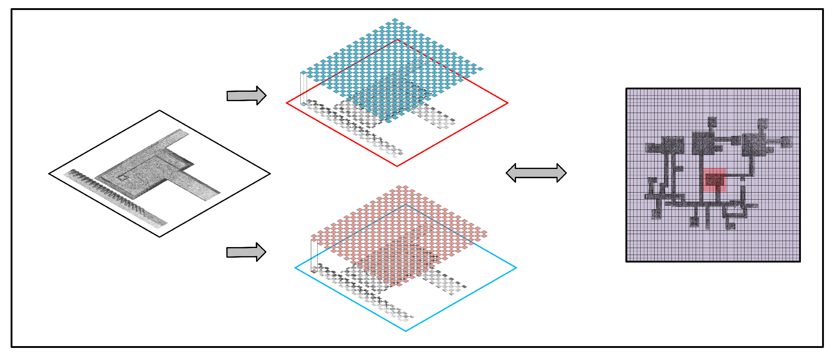
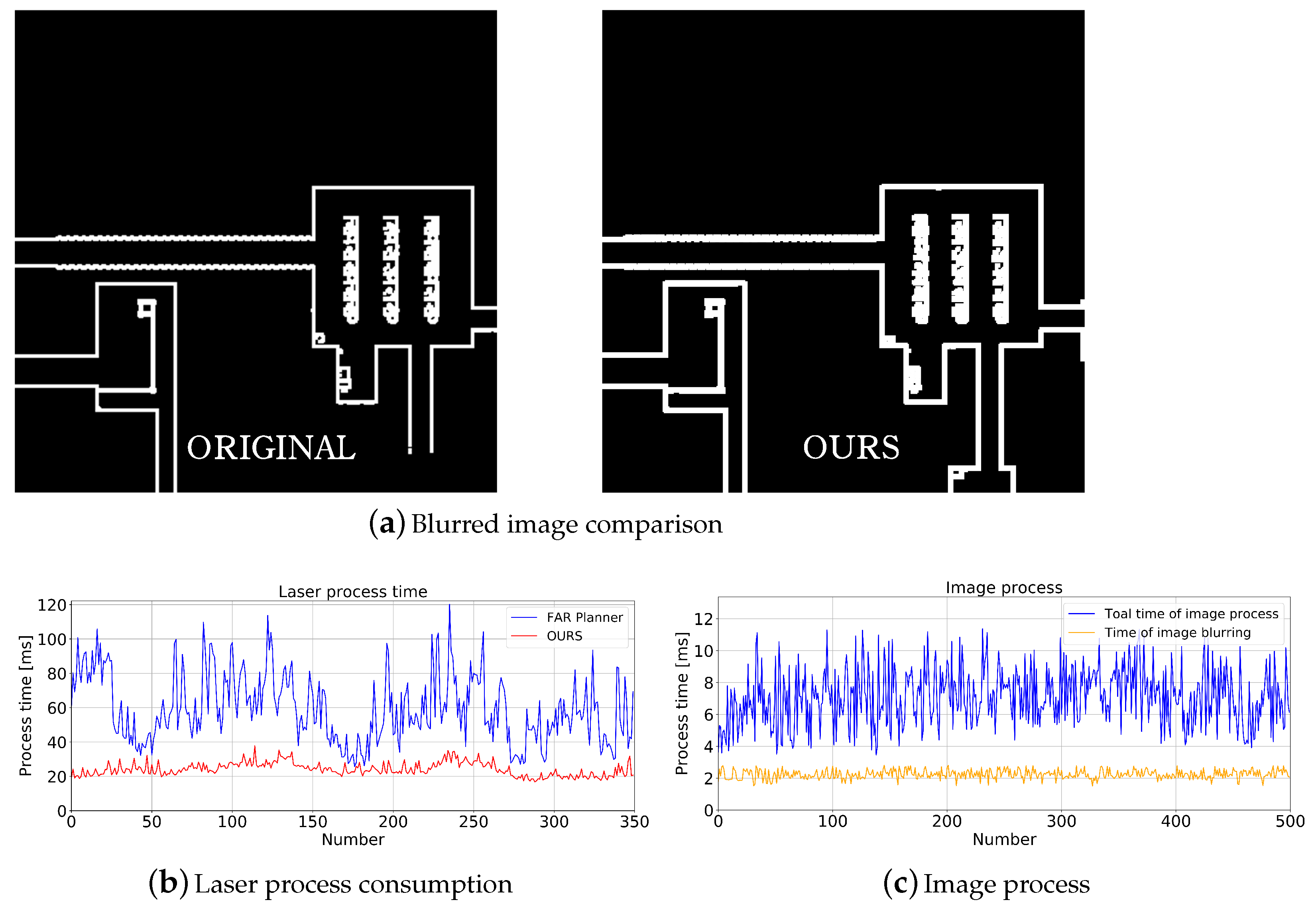
  • Compared to existing methods for storing a laser pointcloud, this paper proposes a complementary holed structure for iteratively updating the local grid. Basically, only half of the pointcloud data needs to be processed in each data frame to update the map. The pointcloud data are subjected to image blurring after planar mapping, and then key vertices are extracted from the blurred image.
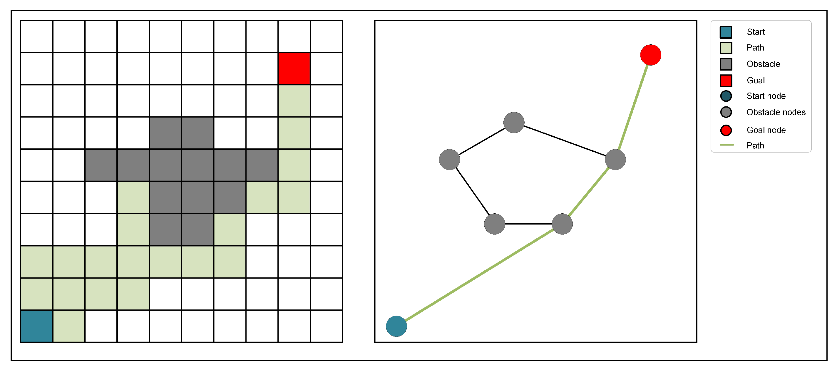
  • For obstacles with complex contours, this paper proposes a filtering method based on the edge length and the number of vertices of the obstacle contour. The method effectively reduces the number of vertices in the v-graph and the maintenance cost of the v-graph by performing vertex filtering on large complex obstacles. Since the v-graph and the path search algorithm are tightly coupled, the efficiency of the path search algorithm will also be improved.
  • A bidirectional breadth-first search algorithm was introduced since exploring uncharted territory requires a lot of search space. In this paper, the edge between the goal point and the existing vertices in the v-graph is established by geometric checking. Therefore, the bidirectional breadth-first search algorithm could reduce the waste of exploration space in navigation.

2. Related Work

The current mainstream of path planning research is divided into the following categories: search-based, sampling (probability)-based, genetic algorithm (GA)-based, and learning-based. According to the planning results, it is further divided into complete planning algorithms and probabilistic complete planning algorithms.
Search-based planning methods: These methods mainly include Dijkstra [22] and its variants, such as A* [23], D* [24], etc. The Dijkstra and A* algorithms are often used to search on discrete grids. Such algorithms are re-initialized for each search cycle, thus taking a long time to plan routes. An incremental version of the Dijkstra-derived algorithm was proposed to reduce re-planning time by adjusting the local information to the planning result in the previous cycle. However, similar to D* Lite [25], when encountering complex environments, the computational load of the incremental algorithm to re-evaluate the current environment is even greater than that of A* without increment. Many improved A* algorithms have been proposed to decrease the memory space and achieve a better trajectory [26,27], but they are all based on the occupancy grids and thus cannot avoid the shortcomings of the occupancy grids.
Random sampling planning methods: These methods mainly include rapidly expanding random tree (RRT) [28] and a series of its variants, such as RRT* [29], informed RRT* [30], and RRT-Connect [31]. These methods are designed for a known environment. Some algorithms derived from RRT are used for planning in an unknown or partially known environment. These methods must perform maintenance or regeneration of random trees frequently to account for newly observed environments.
Genetic algorithm methods (GA): This algorithm performs path planning through crossover and mutation of chromosomes. Tu et al. [32] proposed a method for generating collision-free paths based on GA. Chen et al. [33] proposed an improved GA to minimize the total distance of the UAV. The method in [34] combined deep learning and GA to design a followable path for multi-robots. Moreover, there are many different improvements to GA [35,36,37] to achieve better results. In the genetic algorithm, the choice of parameters such as crossover rate and mutation rate has a significant impact on the quality of the solution, but these values are typically chosen based on experience.
Planning by deep learning: These methods [38,39,40] require a large number of ground-truth labels for training. For example, the essence of training based on deep learning is to encode and decode environmental information. During testing, these methods can handle scenarios similar to the training environment; the essence of training based on reinforcement learning is to encode and map the information of the state of motion every time. During testing, the results are output according to the encoded motion state information. GuichaoLin et al. [41] proposed a collision-free model based on deep reinforcement learning to allow robots to avoid obstacles. Tutsoy et al. [42] provided a minimum time path for a balancing task through reinforcement learning, and [43] considered the energy consumption to design a general dynamic control model based on deep reinforcement learning. However, learning-based methods are inherently data-driven, and the magnitude of the data limits their ability to scale to different environments.
The majority of the aforementioned path planning techniques, including common search-based algorithms, RRT algorithms, and evolutionary algorithms, are based on occupancy grids. When the scope of the searched scene is large, the drawbacks of occupancy grids will constrain the speed of these algorithms, i.e., as shown in Figure 1, in a 10 × 10 grid map, the algorithm based on the occupancy grid map traversed 20 grids to reach the goal, while the algorithm based on the v-graph only traversed five vertices of the obstacle. This paper mainly studies the visibility graph-based and path-planning methods. Although the literature [13,44,45,46] studied the use of the visibility graph for robot navigation, and FAR Planner [19] applied the theoretical part to the exploration and navigation of the actual 3D world, the maintenance of a graph in complex situations is still expensive, and the way-point generated in unknown environments is easy to detour. In order to address these issues, a sparse v-graph path planner is proposed. This path planner enhances the efficiency of v-graph building while decreasing space waste and v-graph maintenance costs.
Similar to FAR Planner [19], the pointcloud is extracted from obstacles and mapped into polygons, from which vertices and edges are extracted to construct the v-graph for navigation. The improvement of our approach is that each data frame of pointcloud in the local area does not fully participate in the construction of the global layer. The complementary hole structure for iteratively updating the local grid is used to store the pointcloud information in the current local area, which means that only half of the points in each data frame need to be processed each time. The method continuously updates the pointcloud information on each data frame until a global map is formed. Compared with the original algorithm of FAR Planner, the proposed algorithm can reach the target point within a shorter distance and take less time.
In simulation experiments, the feasibility of the method is evaluated through the simulated physical environment. The environment of the simulation experiment includes medium-scale, complex-scale, and large-scale environments in the Autonomous Exploration Development Environment provided by CMU [47], and medium-scale indoor environments and complex large-scale indoor environments provided by Matterport3D [48]. In the physical experiment, the LiDAR, and an Inertial Measurement Unit (IMU) are coupled to generate state estimation of the mobile robot [4], and the proposed replacednavigationnavgiation algorithm will be tested in a real garage.

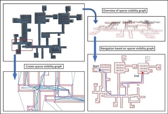
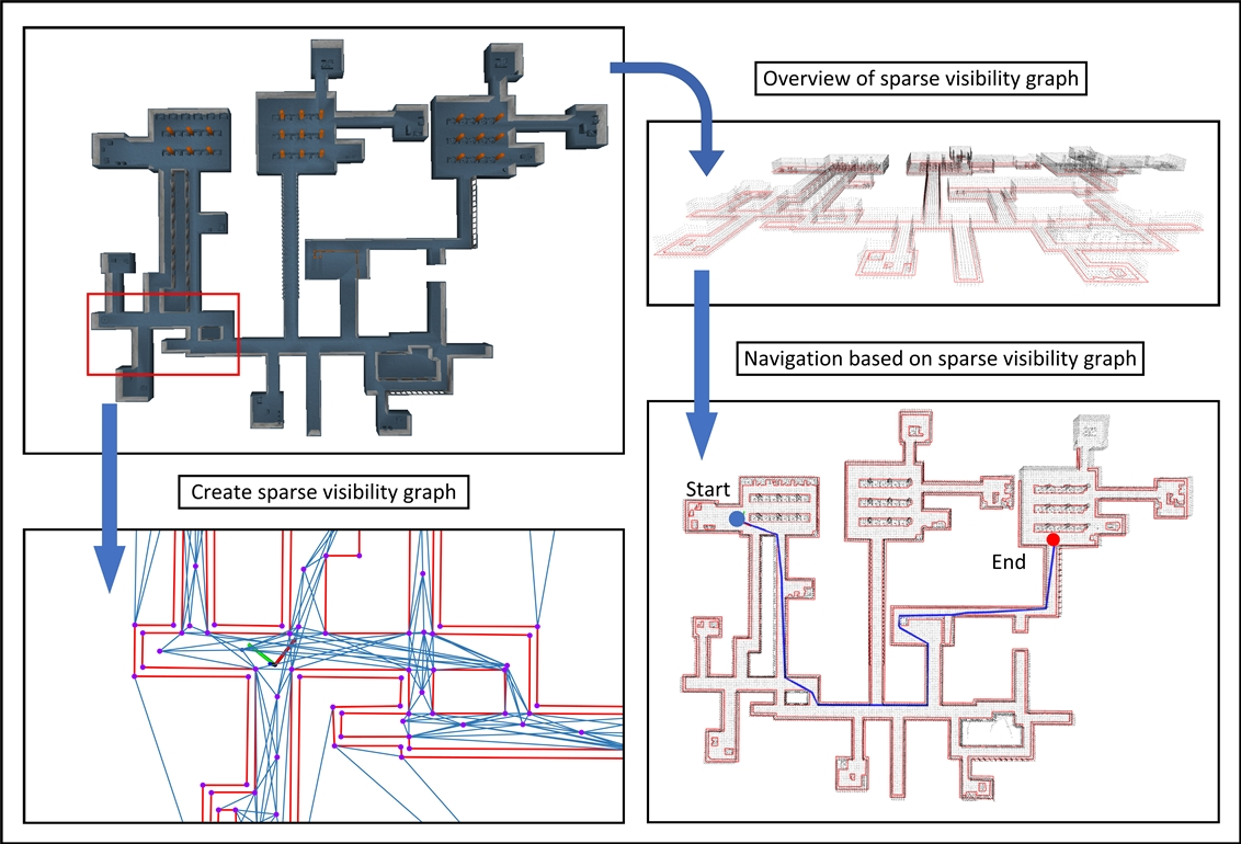
3. Sparse Visibility Graph-Based Path Planner

Define Q R 3 as the robot navigation space, and  S Q as the sensor data from obstacles. A down-sample strategy is used to update and maintain the v-graph, denoted as G , and the grid to store pointcloud is denoted as L . Define the position of robot as P r o b o t Q , the goal P g o a l Q .
The flow chart of the path planner proposed in the paper is shown in Figure 2. And the process consists of three parts: (1) generating the geometric contours of obstacles by LiDAR-to-plane mapping; (2) aggregating and simplifying complex obstacle information to maintain the v-graph at a low cost; and (3) searching for nodes and edges to generate the path from the start point to the goal through the v-graph.

3.1. Pointcloud Extraction Structure

We denote the process of extracting and mapping the pointcloud to geometric contours as extract P c l o u d k Q k Z + , and the grid as G r i d , respectively. In most laser-based SLAM, grids are used for accessibility analysis, which means that pointcloud information needs to be recorded in the global layer L g l o b a l and local L l o c a l . Although an incremental method of updating the pointcloud is proposed, in the case of complex terrain and high-resolution grids, the computational resources used to update the pointcloud are still very high. Therefore, a general sparsification module denoted as F is used to create the holed-structure local grid and incrementally update the pointcloud.
The dilated convolutional module [49] is usually used in neural networks to enlarge the receptive field in the picture, and its whole structure gives another way to deal with the pointcloud in the local grid: as shown in Figure 3, the pointcloud will be stored in the complementary hole grid.
The holed-structure local grid is defined as G r i d d , and the F contains S u b G r i d d ; when obstacles are detected by the LiDAR, the sensor data S is transferred to S u b , all S u b forms the G r i d d . We denote the voxel size as V S , and this value will affect the density of pointcloud. In this paper, the value of V S is set to 0.15 m. When the G r i d d is formed, a PCL filter with a kernel size of ( V S , V S , V S ) will be applied to reduce the size of the pointcloud. S is the remaining pointcloud in the G r i d d . After the local pointcloud is formed, the  S are classified as obstacles or free, and we denote the classified S as P c l o u d k . At this step, the fully classified G r i d d is denoted as L l o c a l , then integrates L l o c a l to L g l o b a l . The complementary hole grids will be generated respectively in different data frames, so that the final L g l o b a l still contains all the information of the pointcloud. The module F is shown in Algorithm 1.
Algorithm 1 Module F .
Input: Sensor data S
Output:  S
    1:
i n p u t   S
    2:
for  e v e r y d a t a f r a m e   do
    3:
    Generate G r i d d
    4:
    for  e a c h S u b  ⊂  G r i d d  do
    5:
         s t o r e p o i n t c l o u d  ∈  S
    6:
    end for
    7:
end for
    8:
A p p l y P C L f i l t e r t o p o i n t  ∈  G r i d d
    9:
c l a s s i f y p o i n t  ∈  G r i d d
    10:
S r e m a i n p o i n t c l o u d i n G r i d d
    11:
U p d a t e G r i d d t o   L l o c a l
As shown in Figure 4, the S u b is a cell in the grid, and it stores a part of the pointcloud information in the 3D space. The standard practice is to form a grid from all cells, but in this paper, a grid with holed structure, as shown in Figure 5a,b, is used to let only part of the cells participate in the calculation. In fact, for a grid of a certain size, the number of cells depends on its resolution. As shown in Figure 6, the higher the resolution, the more cells there are, and the denser the grid, the better its mapping effect. However, the amount of computation increases dramatically. Therefore, this kind of holed-structure grid can save the calculation cost very well because it mainly requires half cells to participate in the calculation in each data frame.
For the obstacle extraction process and obstacle vertices reconstruction process in the v-graph, the sensor information S is gridded and stored by the module F to obtain S . After that, the  S will be converted to a binary image I . To enhance robustness, the image I will be blurred, then obstacle vertices will be extracted through image processing [50] to generate polygons P c o n t o u r k Q k Z + . The polygon extraction algorithm is shown in Algorithm 2.
To define the kernel size of the box filter in Algorithm 2, the equation is as follows, where  R W and R L are the width and length of the robot, respectively, and  V S is the voxel size. In this paper, V S is set to 0.15 m:
( k e r n e l w i d t h , k e r n a l h e i g h t ) = m a x ( m a x ( R W , R L ) 2 + V S V S , 5 )
Figure 7 demonstrates the blurred picture of LiDAR-mapped obstacle geometry and the time consumption of the laser process. As can be seen from Figure 7a, the hollow structure (using module F ) does not affect the image after blurring. Compared with the original (without using a hollow structure), it can be found that our generated contour approximates the original image. The projected outline of the obstacle is thicker because of the blurred image, and the details inside the outline are lost.
The time required for the laser process, according to Figure 7b, includes gathering the raw pointcloud and downsampling. For the same area, the time consumed by using the holed structure is more gentle, while the processing process without the holed structure is steeper and its curve fluctuates greatly. The time it takes to process an image is depicted in Figure 7c. The total time of the image process includes mapping the pointcloud in L l o c a l into the image I , blurring the image, and initially extracting the obstacle contour points. About 20% of the total image processing time is spent on blurring the outline of obstacles.
Algorithm 2 Polygon Extraction.
Input:  S  ∈  L l o c a l
Output:  P o l y g o n s :   P c o n t o u r k
    1:
i n p u t   S
    2:
C r e a t e b i n a r y i m a g e   I   f r o m p o i n t s i n   S
    3:
A p p l y b o x f i l t e r   w i t h k e r n a l s i z e o f ( k e r n e l   w i d t h , k e r n a l h e i g h t ) t o b l u r i m a g e   I
    4:
E x t r a c t p o l y g o n s   P c o n t o u r k   b a s e d o n [50]
    5:
for  e a c h   P c o n t o u r k   do
    6:
     D o w n s a m p l e v e r t i c e s i n   P c o n t o u r k   b a s e d o n [51]
    7:
end for

3.2. Simplified Complex Contours Algorithm

In the previous Section 3.1, the  L was constructed to obtain the pointcloud from LiDAR. In this section, the polygons will be extracted and simplified based on L .
For the graph update method of the two-layer architecture, shown in Figure 8, we define G l o c a l and G g l o b a l . Between them, G l o c a l is the local layer around the robot, and  G g l o b a l is the layer set of the entire observation environment. G l o c a l will be generated by the sensor information S for each data frame and then merged into G g l o b a l For each data frame, the sensor information S will generate G l o c a l and then be merged with G g l o b a l , noting that since the module F is used to store the sensor information S , now S  ∈  L l o c a l can be used to merge G g l o b a l at a lower cost.
It is known that the computational complexity involved in constructing a v-graph is O( n 2 log n ) [52], where n is the number of vertices in the graph. In normal case, the cost of building a local graph in the environment is small enough so that computational resources can be allocated to each data frame in an incremental update manner. However, redundant nodes will also be generated during each v-graph update if the environment has numerous complex obstacles, leading to a significant increase in the number of edges connecting the nodes. To ensure the effectiveness of the v-graph update, a method for further sparse operation on complex contours is required.
Constructing local layers: The S  ∈  L l o c a l will be converted into local polygons P c o n t o u r k , and use P c o n t o u r k to construct a local visualization graph G l o c a l . Note that for complex polygons, as shown in Figure 9, the polygon contains many vertices composed of short edges. Adding redundant vertices will construct more useless edges; thus, a lot of computing resources are wasted on unnecessary vertices and edges in the process of path search in complex terrain.
A threshold η is set to control the number of vertices for complex large local polygons. When the number of vertices of the polygon P c o n t o u r k is greater than η , the vertices will be reduced, which not only optimizes the geometric outline of large and complex obstacles, but also retains the geometric characteristics of small obstacles. As shown in Figure 10, the continuous vertices inside those red circles in Figure 10a should be eliminated, but the current method does not eliminate them well, resulting in more vertices and edges in the v-graph. Compared to Figure 10a, the optimized version in Figure 10b has fewer vertices.
When the number of vertices of an obstacle is greater than η in the local layer, the algorithm preferentially records the distance between the two longest vertices in the obstacle. For example, the distance between the longest two vertices is d i s t m a x . The algorithm traverses the three consecutive vertices v e r t e x i 1 , v e r t e x i , v e r t e x i + 1 in the obstacle and calculates the length between the two vertices, respectively. The distance between them is denoted as d i s t ( i , i 1 ) and d i s t ( i , i + 1 ) . If both d i s t ( i , i 1 ) and d i s t ( i , i + 1 ) are less than 0.1 ×  d i s t m a x , it means that v e r t e x i is an invalid vertex (excess vertex), in which case we delete v e r t e x i and destroy its connection edges e d g e ( i 1 , i ) and e d g e ( i , i + 1 ) .
Since the simplified complex contours algorithm only works on the G l o c a l , the v-graph update process will not be slowed down by the accumulation of the number of nodes in the G g l o b a l .
Update the global layer: After G l o c a l is constructed, the  G l o c a l and the G g l o b a l are fused. The strategy is: take out the overlapping parts of G l o c a l in G g l o b a l , and associate the vertex position in the G l o c a l to the G g l o b a l . The Euclidean distance is used to associate vertices in two layers, and the associated vertices are recorded. The entire graph updating algorithm is as follows in Algorithm 3, and the final obstacle contours and edges are shown in Figure 11.
For the given two points a ( a x , a y , a z ) and b ( b x , b y , b z ) , the  d i s t a n c e ( a , b ) in Algorithm 3 is defined as followed:
d i s t a n c e ( a , b ) = ( a x b x ) 2 + ( a y b y ) 2 + ( a z b z ) 2
Algorithm 3 Visibility Graph Update.
Input:  S  ∈  L l o c a l , g r a p h   G
Output:  U p d a t e g r a p h   G
    1:
P c o n t o u r k  ←  P o l y g o n E x t r a c t i o n ( S ); // f r o m A l g o r i t h m   2
    2:
for  e a c h   P c o n t o u r k   do
    3:
    if  t h e n u m b e r o f v e r t i c e s  >  η  then
    4:
        for  e a c h   v e r t e x   i n   c o n t o u r  do
    5:
            d i s t m a x = m a x ( d i s t a n c e ( v e r t e x i , v e r t e x i + 1 ) )
    6:
        end for
    7:
        while  t r u e  do
    8:
           for  e a c h   v e r t e x   i n   v e r t i c e s  do
    9:
                 d i s t ( i , i 1 ) = d i s t a n c e ( v e r t e x i 1 , v e r t e x i )
    10:
               d i s t ( i , i + 1 ) = d i s t a n c e ( v e r t e x i , v e r t e x i + 1 )
    11:
              if  d i s t ( i , i ± 1 )  <  0.1 × d i s t m a x  then
    12:
                    E l i m i n a t e v e r t e x i
    13:
                    E l i m i n a t e u n n e c e s s a r y e d g e ( i 1 , i ) a n d e d g e ( i , i + 1 )
    14:
               end if
    15:
           end for
    16:
           if  a l l   d i s t ( i , i ± 1 )  ≥  0.1 × d i s t m a x  then
    17:
                b r e a k
    18:
           end if
    19:
        end while
    20:
    else
    21:
         c o n t i n u e
    22:
    end if
    23:
end for
    24:
A s s o c i a t e v e r t i c e s   P c o n t o u r k   i n t h e   G g l o b a l
    25:
U p a t e t o v i s i b i l i t y g r a p h   G

3.3. Path-Planning Based on Bidirectional Breadth-First Search

In FAR Planner, the goal point P g o a l is used as a vertex, and the Euclidean distance is used as the score to update the parent node of P g o a l . Although the path can be found in an unknown environment, its spatial search range is obviously wasted. The strategy adopted by the robot in many cases is to explore many unnecessary spaces until it finally reaches the goal. As shown in Figure 12, the robot travels from position 0 (start) to position 1, resulting in unnecessary exploration space.
A bidirectional breadth-first search (bidirectional BFS) structure is combined with the v-graph to search for a path, selecting a vertex of a connecting edge of the robot in the forward search while simultaneously beginning a backward search from the P g o a l to find the path to the robot’s current position. This minimizes the amount of unnecessary exploration space.
In the planning, assume that there are no obstacles in the unknown area where the P g o a l is located. The  P g o a l uses geometric collision checking to establish edges with existing vertices P n o d e P n o d e G g l o b a l in the v-graph, and then the P g o a l will be connected to the vertices of the discovered obstacles in the v-graph as shown in Figure 13a. The one-way BFS usually wastes some search space in unknown or partially known environments. This is because the one-way BFS starts from the nodes connected to the robot, calculates the target point according to the cost, and then iterates to the robot position according to the parent node of the target point.
As shown in Figure 13b,c, the one-way BFS enters a fork in the planning of the global path from the starting point to the ending point, resulting in an increase in the search space. The result is shown in Figure 13d, from the red point to the green point, the one-way search wastes a huge amount of space. Therefore, this paper embeds the goal in the v-graph and associates it with the existing vertices in the graph, and adopts a bidirectional breadth-first algorithm for path search.
The bidirectional BFS structure shows in Algorithm 4, in which the two BFS are divided into forward and backward according to the direction of the search (forward searches from the robot position to the P g o a l , and backward searches from the P g o a l to the robot position).
In the Algorithm 4,  p a r e n t F ( · ) and p a r e n t B ( · ) are the functions returning the forward and backward parent of a node.  Q F and Q B are the min-priority queues in forward and backward ones, respectively, and  Q F is ordered by g F , Q B is ordered by g B μ is the cost of the best path found so far (initially,  μ is set to ). Whenever the robot reaches a node and expands in the other search,  μ will be updated if a better path goes through the node. g F is the current distance from start and g B is the current distance from P g o a l t o p F and t o p B are the distances to the top nodes in the forward and backward queues, respectively. The STEP function in Algorithm 5 is responsible for advancing the search through the v-graph and updating μ .
One of the benefits of bidirectional search is that it can, to some extent, avoid the wasted search space caused by entering invalid forks. As shown in Figure 13e, the globally planned path no longer passes through the fork, thus avoiding excessive searching. As a result, as shown in Figure 13f, compared to Figure 13d, the distance traveled by the robot is greatly reduced.
It is not possible to use a vertex that has just been extracted from the v-graph G as a point of navigation directly; instead, a transform is used to turn the vertex into a way-point. As Figure 14 shows, in the obstacle where the point is located, the vertices connected to the point at the polygon will be extracted to calculate the direction vector of the point (in Algorithm 6, they are d i r f r o n t and d i r b a c k , respectively, and the direction vector of the point is the s u r f d i r ).
A detailed description is shown in Algorithm 6. In Algorithm 6, the parameter of s e a r c h d i s t is set to constrain the searching area, and the n e a r d i s t is a step parameter which extends the way-point from s u r f d i r direction, and  R W and R L are the width and length of the robot, respectively. When the way-point extends, the  m a x e x t e n d is set to constrain the length of the extension. The  N e a r O B S ( · ) function is to obtain a range of obscloud from L g l o b a l , with  P w a y p o i n t as center and s e a r c h d i s t as the radius.  C h e c k _ C o l l i s i o n is used to detect if the expanded P w a y p o i n t collides with surrounding obstacles, and the detail of the C h e c k _ C o l l i s i o n function is shown in Algorithm 7.
Algorithm 4 Bidirectional BFS.
Input:  P s t a r t , P g o a l , V i s i b i l i t y G r a p h : G
Output:  p a t h :   P p a t h
    1:
Q F , Q B  ←  m a k e m i n p r i o r i t y q u e u e s f o r t h e n o d e s i n i t i a l l y c o n t a i n i n g o n l y   P s t a r t   a n d   P g o a l
    2:
e x p a n d e d F , e x p a n d e d B  ←  m a k e f o r w a r d a n d b a c k w a r d l o o k u p t a b l e s
    3:
s e a r c h F  ←  ( Q F , e x p a n d e d F , p a r e n t F )
    4:
s e a r c h B  ←  ( Q B , e x p a n d e d B , p a r e n t B )
    5:
μ  ← 
    6:
i n i t i a l i z e   G , a s s o c i a t e   P g o a l   i n   G
    7:
p a t h  ←  n o n e
    8:
while  t o p F + t o p B < μ   do
    9:
    if  a t l e a s t o n e q u e u e i s n o n e m p t y  then
    10:
         c h o o s e t h e s e a r c h t o a d v a n c e
    11:
    else
    12:
        return p a t h
    13: 
    end if
    14: 
    if f o r w a r d s e a r c h w a s c h o s e n then
    15: 
         ( p a t h , μ )  ← STEP ( s e a r c h F , s e a r c h R , p a t h , μ )
    16: 
    else
    17: 
         ( p a t h , μ )  ← STEP ( s e a r c h R , s e a r c h F , p a t h , μ )
    18: 
    end if
    19: 
end while
    20: 
return p a t h
Algorithm 5 STEP ( s e a r c h 1 , s e a r c h 2 , s o l u t i o n , μ ) .
    1:
// 1 denotes the chosen direction and 2 is other direction
    2:
// c ( · ) is the cost function, in this paper, manhattan distance is used
    3:
// c ( u , v ) =   | u x v x |   +   | u y v y |   +   | u z v z |
    4:
μ p o p t h e m i n g 1 n o d e f r o m Q 1
    5:
for  v p a r e n t 1 ( u ) do
    6:
       if  v e x p a n d e d 1 Q 1 o r g 1 ( u ) + c ( u , v ) < g 1 ( v )  then
    7:
             g 1 ( v ) g 1 ( u ) + c ( u , v )
    8:
            Add v to Q 1
    9:
            if  v e x p a n d e d 2 a n d g 1 ( v ) + g 2 ( v ) < μ  then
    10:
                 p a t h r e c o n s t r u c t t h e p a t h t h r o u g h u a n d v
    11:
                 μ g 1 ( v ) + g 2 ( v )
    12:
            end if
    13:
       end if
    14:
       return ( p a t h , μ )
    15: 
end for
In Algorithm 6, the  n o r m a l i z e ( P a , P b ) and n o r m a l i z e ( · ) are defined as followed:
n o r m a l i z e ( P a , P b ) = P b P a | | P b P a | |
n o r m a l i z e ( V ) = V | | V | |
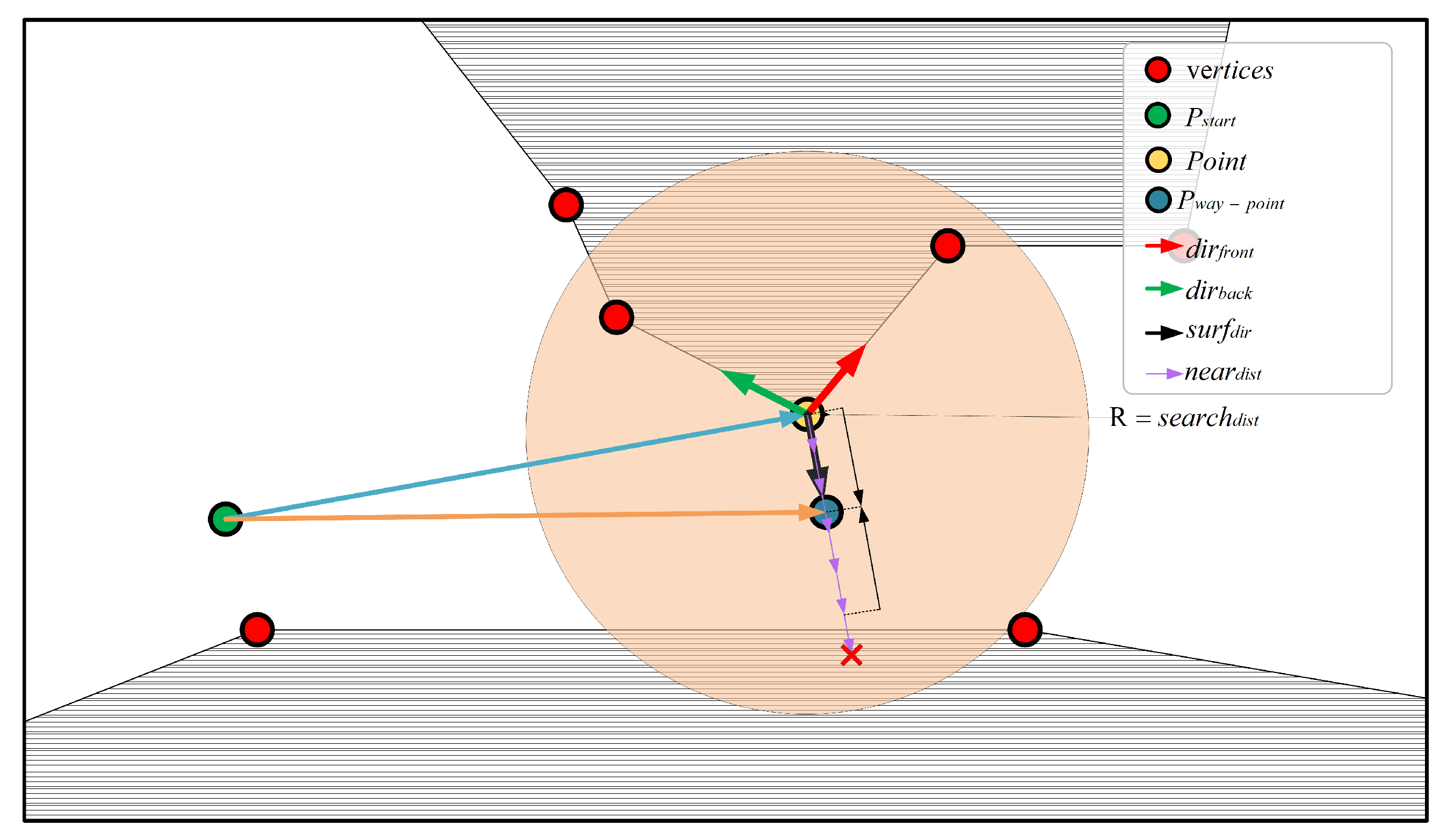
Algorithm 6 Way-point generation.
Input:  P s t a r t , P a t h , L g l o b a l
Output:  P w a y p o i n t
    1:
v e r t e x = P a t h [ 0 ]
    2:
P a t h = P a t h [ 1 : ]
    3:
s e a r c h d i s t = m a x ( 2.5 × m a x ( R L , R W ) , 5 )
    4:
n e a r d i s t = m i n ( m i n ( R L , R W ) , 0.5 )
    5:
P w a y p o i n t = v e r t e x
    6:
m a x e x t e n d = m i n ( s e a r c h d i s t , d i s t a n c e ( P s t a r t , P w a y p o i n t )
    7:
d i r f r o n t = n o r m a l i z e ( p o l y g o n k ( i 1 ) , p o l y g o n k ( i ) )
    8:
d i r b a c k = n o r m a l i z e ( p o l y g o n k ( i + 1 ) , p o l y g o n k ( i ) )
    9:
if  P w a y p o i n t i s a c o n v e x p o i n t   then
    10:
     s u r f d i r = n o r m a l i z e ( d i r f r o n t + d i r b a c k )
    11:
else
    12:
     s u r f d i r = n o r m a l i z e ( d i r f r o n t + d i r b a c k )
    13:
end if
    14:
o b s c l o u d = N e a r O B S ( L g l o b a l , s e a r c h d i s t , P w a y p o i n t )
    15:
o b s c l o u d = s e t I n p u t C l o u d ( o b s c l o u d ) //setInputCloud is a pcl library function to build the KDTree of a set of pointcloud
    16:
t e m p = P w a y p o i n t + s u r f d i r × n e a r d i s t
    17:
i s _ c o l l i d e = C h e c k _ C o l l i s i o n ( t e m p , o b s c l o u d ) //from Algorithm 6
    18:
e x t e n d d i s t = n e a r d i s t
    19:
while  i s _ c o l l i d e i s f a l s e a n d e x t e n d d i s t < s e a r c h d i s t   do
    20:
     t e m p + = s u r f d i r × n e a r d i s t
    21:
     e x t e n d d i s t + = n e a r d i s t
    22:
     i s _ c o l l i d e = C h e c k _ C o l l i s i o n ( t e m p , o b s c l o u d )
    23:
    if  e x t e n d d i s t < m a x e x t e n d  then
    24:
         P w a y p o i n t = t e m p
    25:
    end if
    26:
end while
    27:
if  i s _ c o l l i d e i s t r u e a n d e x t e n d d i s t > m a x ( R W , R L )   then
    28:
     P w a y p o i n t = P w a y p o i n t + v e r t e x s u r f d i r × n e a r d i s t 2
    29:
    return P w a y p o i n t
    30: 
else
    31: 
    return d r o p t h i s v e r t e x a n d r e s e a r c h p a t h
    32: 
end if
Algorithm 7 Check_Collision.
Input:  p o i n t  P, o b s c l o u d
Output:  f a l s e o r t r u e
    1:
r a d i u s = n e a r d i s t / 2 + V S
    2:
t h r e = n e a r d i s t / V S
    3:
K D T r e e r a d i u s S e a r c h ( P , r a d i u s , i n d i c e s , d i s ) // search points with P as center and radius as the search radius, return the number of points in indices and the distance between each point and P.
    4:
if  i n d i c e s > t h r e   then
    5:
    return t r u e
    6: 
else
    7: 
    return f a l s e
    8: 
end if

4. Experiments and Results

The paper uses the same experimental parameters as FAR Planner [19], (uniform sensor parameters, the robot speed is set to 2 m/s). A highly complex channel network tunnel, a parking garage with multiple floors, and a forest of trees with many irregularly shaped trees are all included in the simulated experimental environment. The indoor is moderately complex but easy to detour. Additionally, Matterport3D [48] provides a simple environment 17DRP5sb8fy (denoted as 17DR), a slightly complex environment PX4nDJXEHrG (denoted as PX4n), and a large complex environment 2azQ1b91cZZ (denoted as 2azQ).
In the simulation environment, all methods run on a 2.6Ghz i7 laptop, and the v-graph-based methods use images at 0.2 m/pixel resolution to extract points to form polygons. The local layer on the v-graph is in a 40 m × 40 m area with the robot in the center. The threshold of the length of each visibility edge is set to 5 m. Finally, the simulated mobile robot is 0.6 m long, 0.5 m wide, and 0.6 m high.
In the physical environment, ours runs on an embedded device, and the robot speed is set to 0.7 m/s. To adapt to the real environment, the local layer of the v-graph is set to 20 m × 20 m. The length, width, and height of the mobile robot are set as 0.32 m, 0.25 m, and 0.31 m, respectively.

4.1. Simulation Experiment

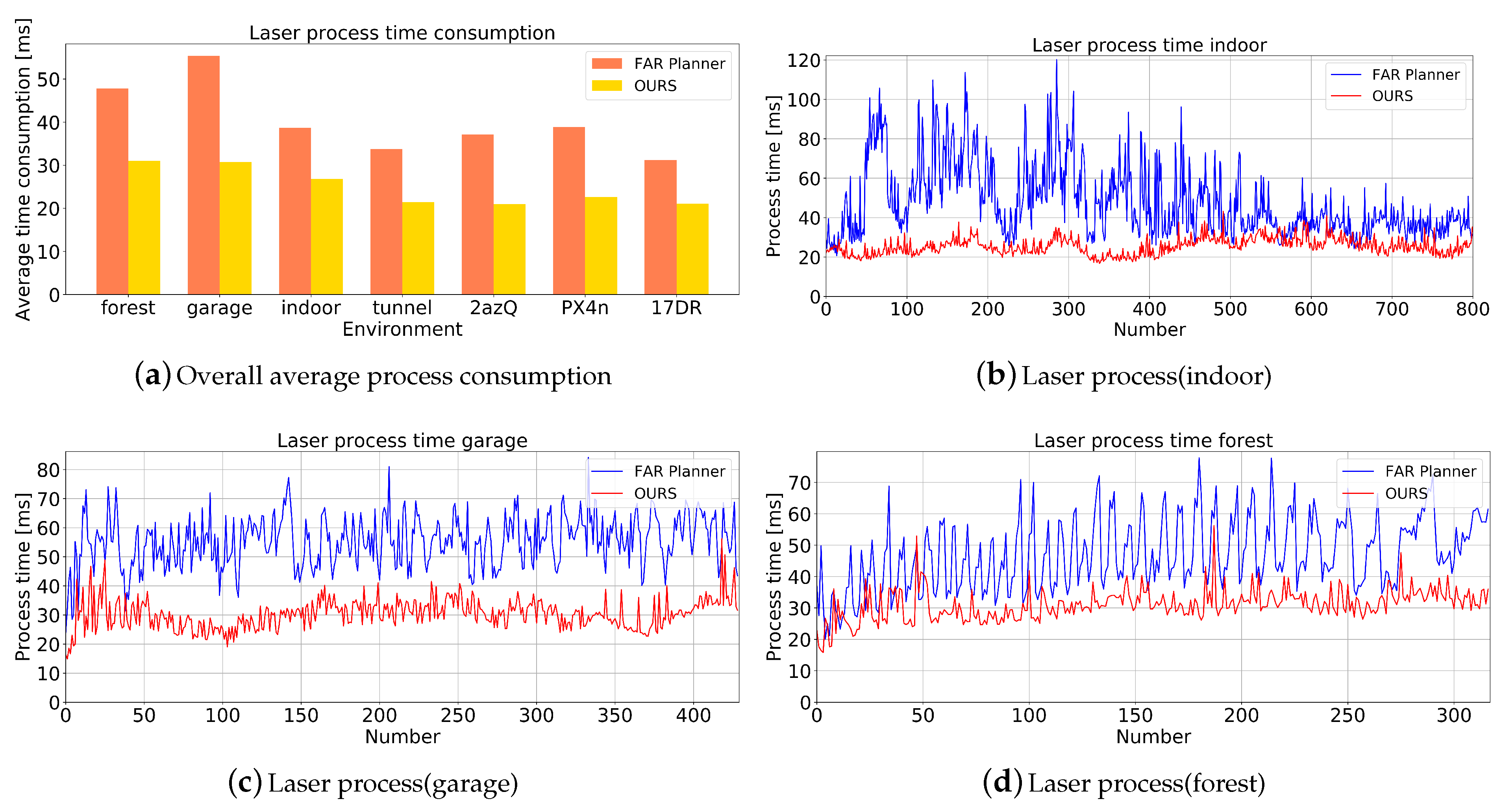
4.1.1. Laser Process Simulation Experiment

In the laser process simulation experiment, seven different types of environments are used to compare the holed structure with the original one. The experimental results are shown in Figure 15. The robot moves according to a fixed route, and the experiment analyzes the time of the laser processing process. The laser processing process refers to the whole process of extracting and storing the pointcloud information of the local layer into the grid and classification (obstacle pointcloud or free pointcloud).
As shown in Figure 15, for example, in the indoor environment, the robot will start from 0 (start) and pass through the target points 1, 2, 3, 4, 5, and 6 in sequence. The initial state of the robot is set to be in an unknown environment, and the known information in the environment is continuously accumulated through exploration. The program records the time of receiving and processing the pointcloud data from LiDAR during the movement of the robot.
Figure 16a is a summary of the average time of laser processing in different environments. It can be clearly seen from Figure 16a that our method used less time in the processing of the pointcloud information in every data frame. Figure 16b–h show that using the grid with the holed-structure leads to the smooth processing of the laser pointcloud. Compared with the original grid, the use of the holed structure can improve the processing speed of the pointcloud by 30.5∼44.5%.

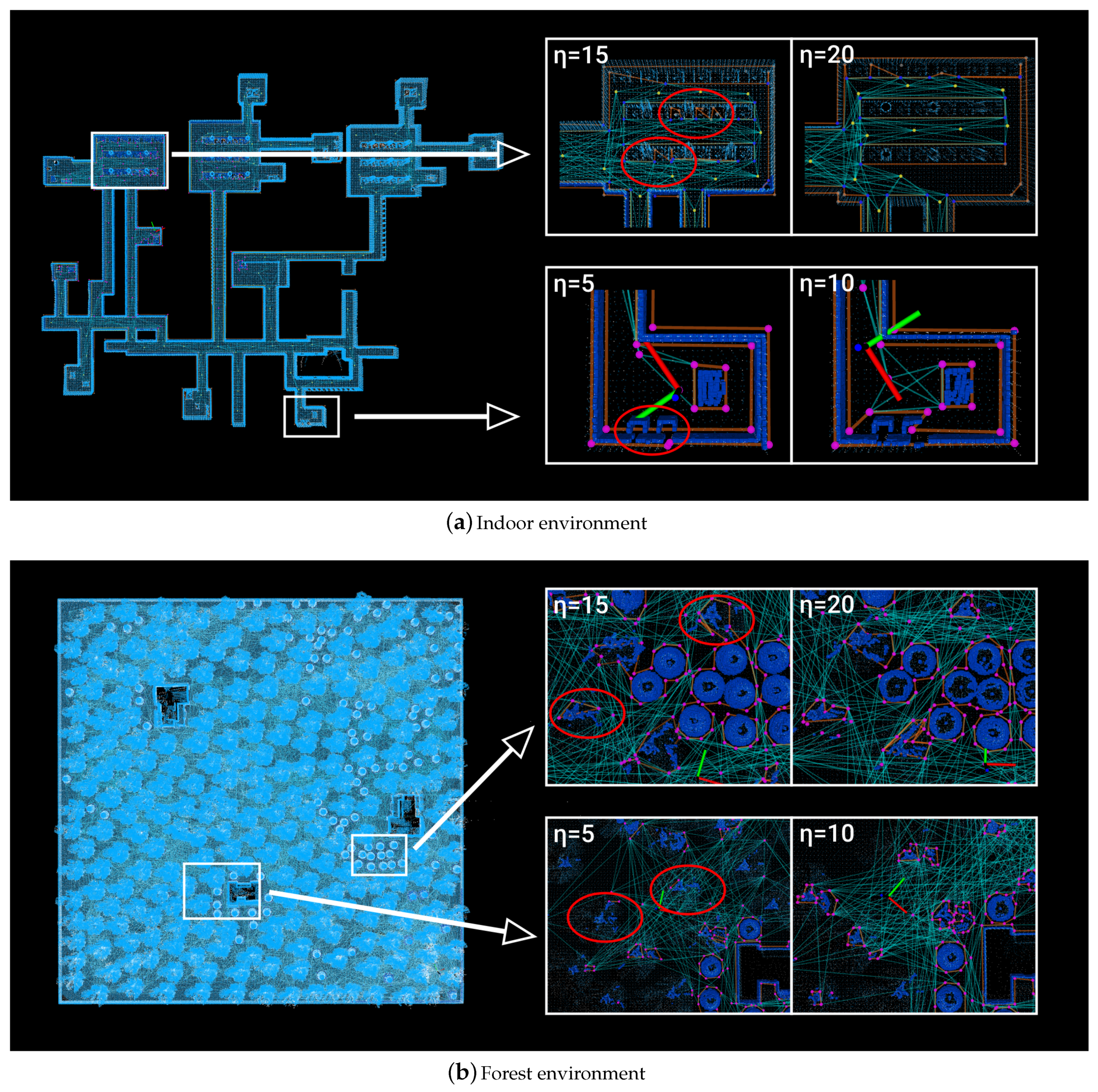
4.1.2. Visibility Graph Update Simulation Experiment

Different values of η , ranging from 5 to 25, are set in representative indoor and outdoor environments in order to select an appropriate value. The robot in the simulation experiment travels throughout the entire environment to count all of the vertices in the v-graph and logs the average update speed. As the Table 1 shows, it can be seen that the number of vertices in the v-graph and the update speed of the v-graph are positively correlated with the value of η , but η is not as small as possible.
Theoretically, a smaller η value should lead to fewer vertices in the v-graph. However, a value of η that is too small will have some drawbacks. The function of collision detection may be affected when some minor obstacles are ignored, as shown in Figure 17a, and this phenomenon also occurs in forest environments. When η is equal to 5, there are two small trees missing from the v-graph in Figure 17b. When η is greater than or equal to 15 and less than or equal to 20, with the increase of η , the outline of the obstacle is well guaranteed, and the update speed of the v-graph is also relatively fast. When η is greater than 25, the number of vertices in the v-graph gradually increases toward the direction of none η . After several rounds of testing, a preliminary conclusion can be drawn that when the value of η is between 15 and 20, the algorithm is most suitable for generating obstacle vertices.
In the v-graph update simulation experiment, seven different environments are used to compare our v-graph update method with FAR Planner’s, and the parameter of η is set to 20. In different environments, a series of target points are established for the mobile robot to travel. These points are fixed, and both methods let the mobile robot pass through them in sequence. For example, in the indoor environment, the robot will pass through the six target points 1, 2, 3, 4, 5, and 6 in sequence. During the driving process of the robot, the update speed of the v-graph will be recorded, and similarly, all the vertices in the v-graph will be recorded. The experimental results are shown in Figure 18.
In each environment in Figure 18a, the robot passes through a series of target points, and the known environment information is reset after reaching each target point. Figure 18b shows the optimized nodes and edges for complex irregular objects. For complex obstacles, ours simplifies the vertex information of the obstacle. When the redundant vertices are reduced, the redundant edges will also be correspondingly reduced. As shown in Figure 18b, the cyan and blue edges and red nodes in the optimized v-graph are significantly reduced, respectively.
Figure 18c shows the average speed of the v-graph update, and Figure 18d shows the total number of vertices in the v-graph. For simple terrain and most of the obstacles with simple shapes and corners, such as the tunnel and 17DRP5sb8fy, our method obtains similar results to FAR Planner, and the improvement is only 10∼20%; for large-scale maps containing complex obstacles, such as the forest, 2azQ1b91cZZ, PX4nDJXEHrG, indoor, etc., our method significantly improves the efficiency by 40∼60% compared to FAR Planner.
It is evident from Figure 19 that for environments with complex terrain, our method greatly reduces the number of vertices for obstacles in the v-graph. In Figure 19e,f, the original method has a total of 73 vertices while our method has only 49 vertices.

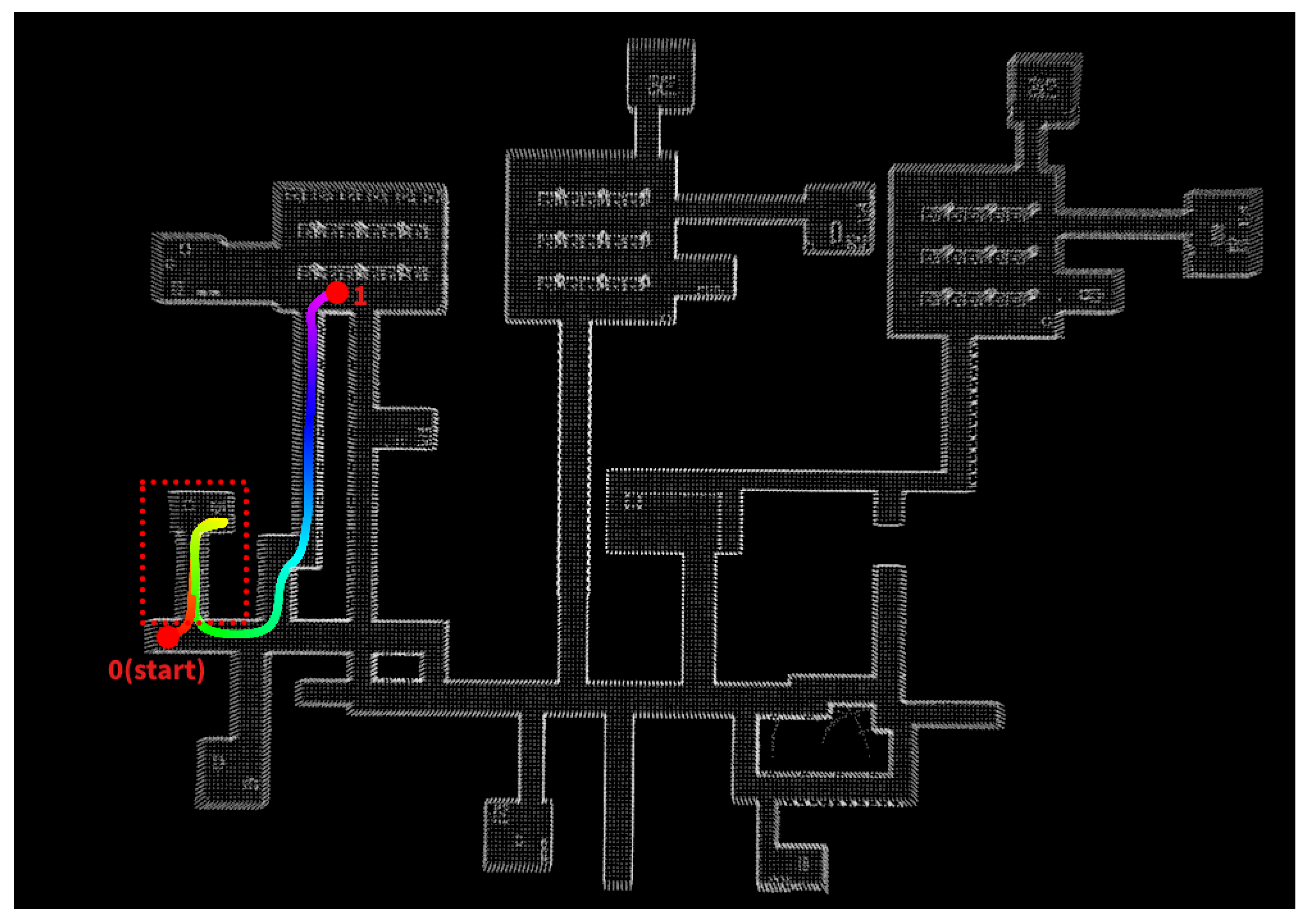
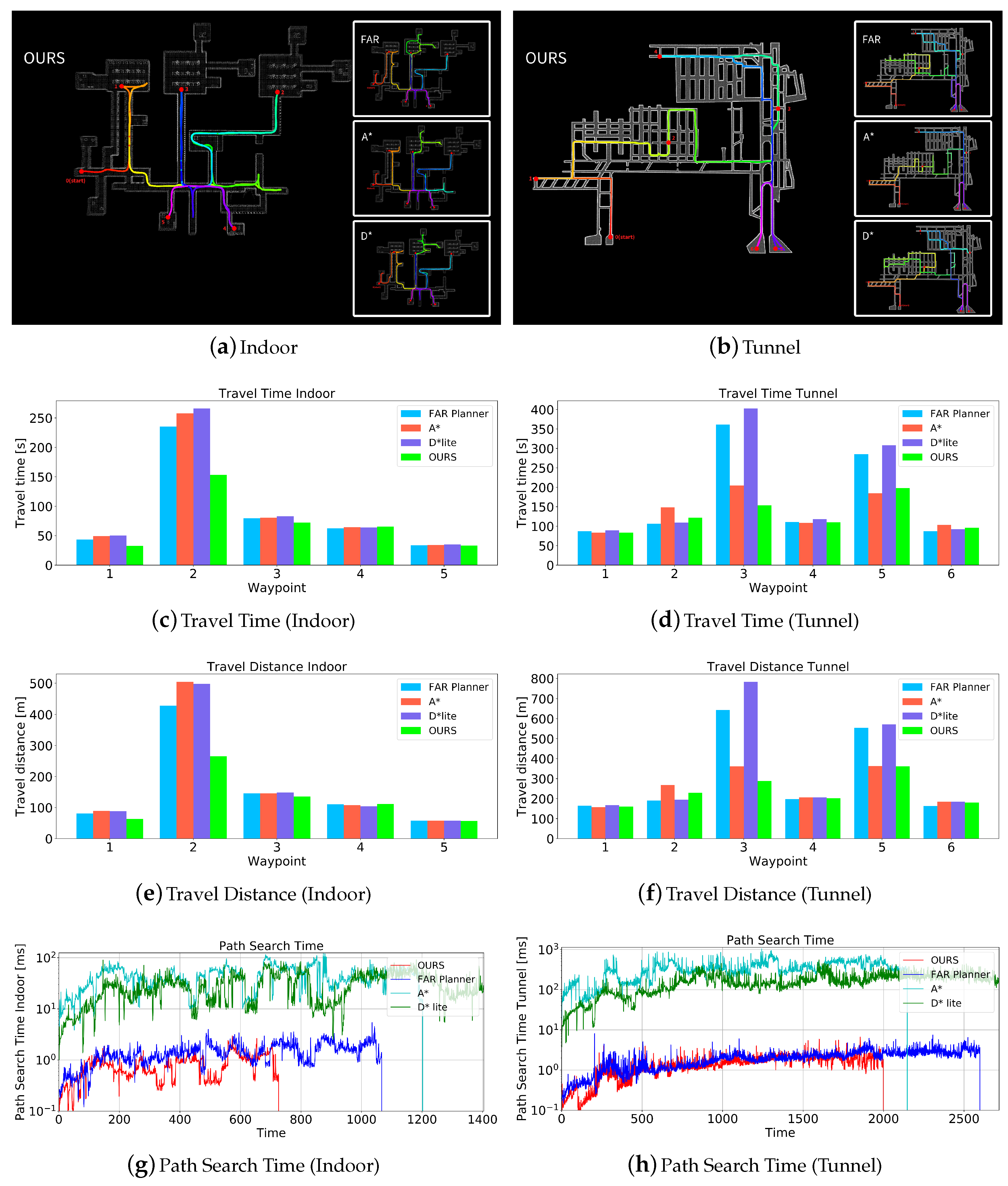
4.1.3. Path Planning Simulation Experiment

For the path exploration in the unknown environment, we compared the slightly complex indoor environment and the tunnel environment with complex network structures, respectively. Similar to the graph update simulation experiment, a series of waypoints are set up in each environment, allowing the robot to pass one by one. Define the robot to accumulate environmental information while exploring the unknown environment.
FAR Planner (v-graph-based), A*, and D* Lite (occupancy grid-based) are all added for comparison with our algorithm. Figure 20 shows the trajectory paths generated by our algorithm and other algorithms in navigation. In the case of reaching the same navigation point, our algorithm can avoid unnecessary exploration space to a greater extent than the FAR Planner and A*, D* Lite, so as to achieve a shorter distance and less time.
Figure 20c–f show the time and distance it takes for the robot to travel from one navigation point to another, and the robot accumulates map information during driving. Table 2 and Table 3 (FAR Planner denoted as FAR) gives a summary of the overall travel time, distance, and search time used for each map robot navigation.
As can be seen from Figure 20a for the indoor environment, the search space is wasted to varying degrees when using FAR Planner, A*, and D* Lite to navigate from point 1 to point 2. They are more inclined to explore the place where point 3 is located and then turn back after finding that there is no passage leading to point 2. The possible reason for this is that most of their cost functions only refer to the cost of the current node itself and the cost of the Euclidean distance between the endpoint and the current node. This causes the robot to tend to drive towards the node with the lowest total cost in a single direction, even though that node may not be able to reach the goal.
For adjacent navigation points with relatively short distances, such as from navigation point 4 to navigation point 5 in an indoor environment, the time and distance consumed by all algorithms are not much different.
The A* and D* Lite are known for their search integrity in finding the optimal path. However, those methods are difficult to scale as the computational cost increases significantly when environments are large and complex [19]. For the tunnel environment, although the environment contains a series of complex #- and T-shaped structures, there are almost no dead ends, that is, the goal can be reached in any direction, so the robot hardly needs to be turned back during the running process. For traditional A* and D* Lite, due to the increase in scene scale, the number of grids that need to be calculated increases sharply, and the cost of algorithm operation increases significantly in large-scale scenes. However, for us, the use of bidirectional BFS allows us to avoid some bifurcations and travel a shorter distance to the destination point.
As shown in Figure 20a,b, our planner is able to search for shorter paths and generate effective trajectories. Table 2 shows that in the indoor case, our method reduces travel time by 23% compared to A*, 28% compared to D* Lite, and 21% compared to FAR Planner’s original algorithm. In terms of increased time, FAR Planner has the most time wasted due to ineffective exploration, while A* and D* Lite are time-consuming when the robot is constantly swinging back and forth in a certain position, but what all three have in common is wasted search space between some navigation points. Table 3 shows that in the tunnel case, our method produces the shortest distance, which is 8% shorter than A*, 32% shorter than D* Lite, and 25% shorter than FAR Planner.
Table 2 and Table 3 show that our planning algorithm can run faster because of the use of a hole-structured mesh to update the graph and vertex optimization for complex obstacles. Compared to FAR Planner, our search algorithm update rate is 43% faster.

4.2. Physical Experiment

The physical experiment uses the mobile robot platform in Figure 21 with the speed set to 0.7 m/s. The mobile robot is equipped with a Velodyne-16 LiDAR and an Inertial Measurement Unit (IMU) 9250. The entire autonomous system is built on Robot Operating System [53], and the Raspberry Pi 4B is the master and the laptop is the slave. In the autonomous system, the master is used to transmit LiDAR data, run the CMU autonomous exploration interface [47], and drive the stm32. The navigation algorithm runs on the slave. The camera at 640 × 480 resolution in the mobile robot is only used to obtain pictures of the environment. The LiDAR and IMU are coupled to generate the state estimation of the robot through Lego-LOAM [4]. The main system structure of the mobile robot is shown in Figure 22, the autonomy system incorporates navigation modules from CMU autonomous development interface, e.g., terrain analysis and way-point following as fundamental navigation modules.
As shown in Figure 23a,b, obstacles are mapped as polygons in exploration, and solid edges are formed from each relevant vertex. In Figure 23c, colored pointclouds of obstacles are displayed to better show the details; orange lines denote the obstacles’ outlines, while cyan lines denote the relationships between the edges of various obstacles.
In the navigation, as shown on the left side of Figure 23d, the mobile robot started from point 1 and arrived at points 2, 3, and 4 in sequence and on the right side of the Figure 23d shows pictures when the mobile robot navigates to the corresponding position.
As shown in Figure 24, our algorithm is compared with FAR Planner in the physical experiment. The processing speed of the laser data, the update speed of the v-graph, and the operation speed of the search algorithm are recorded every 0.5 seconds.
In Figure 24a, The mean and standard deviation for the laser processing of FAR Planner are 60.95 ms and 16.59 ms, respectively, while our method’s mean and standard deviation of the laser processing are 41.59 ms and 9.93 ms, respectively. Not only is ours 31.76% faster on average than FAR Planner, but the time taken by the algorithm is also more stable. As shown in Figure 24b, both approaches will take longer to update the v-graph because of the unexpected rise in obstacles, but ours is on average 37.12% quicker than FAR Planner. In Figure 24c, ours is on average 18.06% faster than the FAR Planner on the search algorithm.

5. Discussion

5.1. Grid in Mapping

In the process of robot simultaneous localization and mapping, grids can be used to store pointcloud data [12,54,55,56,57,58], and can also be used as occupancy grid maps for robot navigation [56,59,60,61,62,63]. As mentioned in Lau, B et al. [58], the processing speed of a computer is limited by the resolution of the grid. When the grid resolution is higher, the information represented by each cell is more accurate, but the calculation time is longer. In Homm et al. [61], they use a Graphics Processing Unit (GPU) to speed up the formation of fine grids, and in A. Birk et al. [56], they use multiple robots to jointly maintain grid maps, an approach that indirectly speeds up the construction of the grid map.
The aim of the work in this paper is to use a discrete hollow grid to convert pointcloud information into a binary image and extract obstacle vertices. Therefore, the focus of this paper is on how to quickly extract the grid to generate the vertices of obstacles. For a 30 m × 30 m local grid, the processing speed of a high-resolution grid, such as 0.5 m × 0.5 m per cell, is much slower than that of a low-resolution grid, such as 1 m × 1 m per cell. Therefore, a grid with spaced hollow structures is designed to speed up the processing of high-resolution grids. Since the use of hollow structures will affect subsequent images, such as the discontinuous edges of obstacles, it is necessary to blur the generated images. Blurring the image can cover empty spots caused by hollow structures. Additionally, a complementary hollow-structured grid is also considered, storing a set of complementary hollow-structured grids under adjacent data frames and integrated into the local map.
It is foreseeable that the grid application with this sparse structure can significantly reduce the amount of computation and shorten the computation time in three-dimensional space. In future work, the authors hope to use this sparse structure for 3D grids.

5.2. The Reduced Visibility Graph

The v-graph is a topology map that is widely used for path planning since it is constructed using the vertices of obstacles. The difficulty of calculating and maintaining the v-graph mainly depends on the number of vertices in the graph; thus, many researchers focus on how to simplify the v-graph [19,64,65,66,67,68,69,70,70].
In Nguyet et al. [69], he proposed a method for clustering small obstacles according to their volume, which can well reduce the number of vertices in the v-graph, thereby improving the efficiency of the path search algorithm. However, this method needs to calculate the total area of the global map for each iteration, which wastes a lot of time for multiple small-volume obstacles. In Yang et al. [19], an angle ζ is set to limit the visibility of each obstacle vertex, which can well reduce the number of edges of the obstacle vertex. The method used in this paper combined Yang’s method [19] and proposed a method of simplifying obstacle vertices that only act on the local map. Compared with [69], the speed of the algorithm proposed in this paper is not affected by the global map, and it effectively reduces invalid vertices and redundant edges.

5.3. Uncertainties in the Path Planning

The path planning is based on the produced map (they can be occupancy maps, topological maps, or semantic maps), and the localization of the robot is very important for constructing the map. In the simulation experiment, we can easily obtain the relevant data of the robot, such as the simulated IMU sensor information and the simulated LiDAR information, and this information is accurate and unbiased in the simulated environment to estimate the state of the robot. How well the robot is positioned determines whether the map used for navigation is available. However, in real life, we cannot obtain such unbiased data; therefore, we used Lego-LOAM for the state estimation of the robot. If the robot’s state estimation data has a large error, the v-graph it builds will deviate from the real world.
As shown in Figure 25, in the real world, the mobile robot made an error in the state estimation, and the white pointcloud newly scanned by the LiDAR was obviously offset from the colored obstacle pointcloud. This will lead to the establishment of an unreliable v-graph, thus affecting the effect of path planning.

6. Conclusions

This paper proposed a sparse visibility graph-based path planner based on the FAR Planner framework. Our method is far superior to the FAR Planner in terms of the efficiency of v-graph maintenance and generation. Our method can be used for navigation in known environments and exploration in unknown environments. Moreover, a complementary hollow grid is designed for local layer updates and merges the local layer into the global layer. For complex obstacles in the environment, a method was proposed to reduce the cost of maintaining the v-graph by simplifying the vertices and edges of polygons. For small obstacles, their information is still preserved in the graph. Moreover, the paper proposed a path planning method based on a bidirectional breadth-first search combined with the v-graph. By comparing the original algorithm of FAR Planner and the traditional search algorithms A* and D* Lite, ours achieves the optimal path planning in unknown environments, and the speed of the path search algorithm is faster than that of FAR Planner.

Author Contributions

Conceptualization, Q.L. and F.X.; methodology, Q.L., F.X., J.Z. and B.X.; software, Q.L., F.X. and J.Z.; validation, Q.L., F.X. and B.X.; formal analysis, F.X., J.Z.; investigation, J.Y.; resources, X.L.; data curation, H.S. and J.Z.; writing—original draft preparation, Q.L. and F.X.; writing—review and editing, Q.L., F.X. and B.X.; visualization, H.S. and J.Z.; supervision, J.Y.; project administration, F.X. and X.L.; funding acquisition, J.Y. All authors have read and agreed to the published version of the manuscript.

Funding

This work was partially supported by the National Natural Science Foundation of China (Grant Nos. 41974033 and 61803208), the Scientific and technological achievements transformation project of Jiangsu Province (BA2020004), 2020 Industrial Transformation and Upgrading Project of Industry and Information Technology Department of Jiangsu Province, Postgraduate Research & Practice Innovation Program of Jiangsu Province.

Data Availability Statement

The CMU simulation environment can be acquired through https://www.cmu-exploration.com. The Matterport3D simulation environment can be acquired through https://niessner.github.io/Matterport. The original framework used in the paper can be acquired through https://github.com/MichaelFYang/far_planner (all accessed on 14 June 2022).

Acknowledgments

The authors would like to sincerely thank all the funders.

Conflicts of Interest

The authors declare no conflict of interest. The funders had no role in the design of the study; in the collection, analyses, or interpretation of data; in the writing of the manuscript, or in the decision to publish the results.

Abbreviations

The following abbreviations are used in this manuscript:
FAR PlannerFast, Attemptable Route Planner using Dynamic Visibility Update [19]
SLAMSimultaneous Localization And Mapping
IMUInertial Measurement Unit
GPUGraphics Processing Unit

References

  1. Hess, W.; Kohler, D.; Rapp, H.; Andor, D. Real-time loop closure in 2D LIDAR SLAM. In Proceedings of the 2016 IEEE International Conference on Robotics and Automation (ICRA), Stockholm, Sweden, 16–21 May 2016; pp. 1271–1278. [Google Scholar] [CrossRef]
  2. Grisetti, G.; Kümmerle, R.; Stachniss, C.; Burgard, W. A Tutorial on Graph-Based SLAM. IEEE Intell. Transp. Syst. Mag. 2010, 2, 31–43. [Google Scholar] [CrossRef]
  3. Li, T.; Pei, L.; Xiang, Y.; Wu, Q.; Xia, S.; Tao, L.; Guan, X.; Yu, W. P3-LOAM: PPP/LiDAR Loosely Coupled SLAM With Accurate Covariance Estimation and Robust RAIM in Urban Canyon Environment. IEEE Sens. J. 2021, 21, 6660–6671. [Google Scholar] [CrossRef]
  4. Shan, T.; Englot, B. Lego-loam: Lightweight and ground-optimized lidar odometry and mapping on variable terrain. In Proceedings of the 2018 IEEE/RSJ International Conference on Intelligent Robots and Systems (IROS), Madrid, Spain, 1–5 October 2018; pp. 4758–4765. [Google Scholar]
  5. Li, J.; Pei, L.; Zou, D.; Xia, S.; Wu, Q.; Li, T.; Sun, Z.; Yu, W. Attention-SLAM: A Visual Monocular SLAM Learning From Human Gaze. IEEE Sens. J. 2021, 21, 6408–6420. [Google Scholar] [CrossRef]
  6. Mur-Artal, R.; Montiel, J.M.M.; Tardós, J.D. ORB-SLAM: A Versatile and Accurate Monocular SLAM System. IEEE Trans. Robot. 2015, 31, 1147–1163. [Google Scholar] [CrossRef] [Green Version]
  7. Mur-Artal, R.; Tardós, J.D. ORB-SLAM2: An Open-Source SLAM System for Monocular, Stereo, and RGB-D Cameras. IEEE Trans. Robot. 2017, 33, 1255–1262. [Google Scholar] [CrossRef] [Green Version]
  8. Qin, T.; Li, P.; Shen, S. VINS-Mono: A Robust and Versatile Monocular Visual-Inertial State Estimator. IEEE Trans. Robot. 2018, 34, 1004–1020. [Google Scholar] [CrossRef] [Green Version]
  9. Chan, S.H.; Wu, P.T.; Fu, L.C. Robust 2D Indoor Localization Through Laser SLAM and Visual SLAM Fusion. In Proceedings of the 2018 IEEE International Conference on Systems, Man, and Cybernetics (SMC), Miyazaki, Japan, 7–10 October 2018; pp. 1263–1268. [Google Scholar] [CrossRef]
  10. Debeunne, C.; Vivet, D. A Review of Visual-LiDAR Fusion based Simultaneous Localization and Mapping. Sensors 2020, 20, 2068. [Google Scholar] [CrossRef] [Green Version]
  11. Nguyen, T.M.; Cao, M.; Yuan, S.; Lyu, Y.; Nguyen, T.H.; Xie, L. VIRAL-Fusion: A Visual-Inertial-Ranging-Lidar Sensor Fusion Approach. IEEE Trans. Robot. 2022, 38, 958–977. [Google Scholar] [CrossRef]
  12. Thrun, S. Learning Occupancy Grid Maps with Forward Sensor Models. Auton. Robot. 2003, 15, 111–127. [Google Scholar] [CrossRef]
  13. Lozano-Pérez, T.; Wesley, M.A. An algorithm for planning collision-free paths among polyhedral obstacles. Commun. ACM 1979, 22, 560–570. [Google Scholar] [CrossRef]
  14. Kitzinger, J.; Moret, B. The Visibility Graph among Polygonal Obstacles: A Comparison of Algorithms. Ph.D. Thesis, University of New Mexico, Albuquerque, NM, USA, 2003. [Google Scholar]
  15. Alt, H.; Welzl, E. Visibility graphs and obstacle-avoiding shortest paths. Z. Für Oper. Res. 1988, 32, 145–164. [Google Scholar] [CrossRef]
  16. Shen, X.; Edelsbrunner, H. A tight lower bound on the size of visibility graphs. Inf. Process. Lett. 1987, 26, 61–64. [Google Scholar] [CrossRef]
  17. Sridharan, K.; Priya, T.K. An Efficient Algorithm to Construct Reduced Visibility Graph and Its FPGA Implementation. In Proceedings of the VLSI Design, International Conference, Mumbai, India, 9 January 2004; IEEE Computer Society: Los Alamitos, CA, USA, 2004; p. 1057. [Google Scholar] [CrossRef]
  18. Wu, G.; Atilla, I.; Tahsin, T.; Terziev, M.; Wang, L. Long-voyage route planning method based on multi-scale visibility graph for autonomous ships. Ocean Eng. 2021, 219, 108242. [Google Scholar] [CrossRef]
  19. Yang, F.; Cao, C.; Zhu, H.; Oh, J.; Zhang, J. FAR Planner: Fast, Attemptable Route Planner using Dynamic Visibility Update. arXiv 2021, arXiv:2110.09460. [Google Scholar]
  20. Pradhan, S.; Mandava, R.K.; Vundavilli, P.R. Development of path planning algorithm for biped robot using combined multi-point RRT and visibility graph. Int. J. Inf. Technol. 2021, 13, 1513–1519. [Google Scholar] [CrossRef]
  21. D’Amato, E.; Nardi, V.A.; Notaro, I.; Scordamaglia, V. A Visibility Graph approach for path planning and real-time collision avoidance on maritime unmanned systems. In Proceedings of the 2021 International Workshop on Metrology for the Sea; Learning to Measure Sea Health Parameters (MetroSea), Reggio Calabria, Italy, 4–6 October 2021; pp. 400–405. [Google Scholar] [CrossRef]
  22. Dijkstra, E.W. A note on two problems in connexion with graphs. Numer. Math. 1959, 1, 269–271. [Google Scholar] [CrossRef] [Green Version]
  23. Hart, P.E.; Nilsson, N.J.; Raphael, B. A formal basis for the heuristic determination of minimum cost paths. IEEE Trans. Syst. Sci. Cybern. 1968, 4, 100–107. [Google Scholar] [CrossRef]
  24. Stentz, A. Optimal and efficient path planning for partially-known environments. In Proceedings of the 1994 IEEE International Conference on Robotics and Automation, San Diego, CA, USA, 8–13 May 1994; Volume 4, pp. 3310–3317. [Google Scholar] [CrossRef]
  25. Koenig, S.; Likhachev, M. Fast replanning for navigation in unknown terrain. IEEE Trans. Robot. 2005, 21, 354–363. [Google Scholar] [CrossRef]
  26. XiangRong, T.; Yukun, Z.; XinXin, J. Improved A-star algorithm for robot path planning in static environment. J. Phys. Conf. Ser. 2021, 1792, 012067. [Google Scholar] [CrossRef]
  27. Zhang, L.; Li, Y. Mobile Robot Path Planning Algorithm Based on Improved A Star. J. Phys. Conf. Ser. 2021, 1848, 012013. [Google Scholar] [CrossRef]
  28. LaValle, S.M.; Kuffner, J.J.; Donald, B. Rapidly-exploring random trees: Progress and prospects. Algorithmic Comput. Robot. New Dir. 2001, 5, 293–308. [Google Scholar]
  29. Karaman, S.; Frazzoli, E. Sampling-based algorithms for optimal motion planning. Int. J. Robot. Res. 2011, 30, 846–894. [Google Scholar] [CrossRef]
  30. Gammell, J.D.; Srinivasa, S.S.; Barfoot, T.D. Informed RRT*: Optimal sampling-based path planning focused via direct sampling of an admissible ellipsoidal heuristic. In Proceedings of the 2014 IEEE/RSJ International Conference on Intelligent Robots and Systems, Chicago, IL, USA, 14–18 September 2014; pp. 2997–3004. [Google Scholar]
  31. Kuffner, J.J.; LaValle, S.M. RRT-connect: An efficient approach to single-query path planning. In Proceedings of the 2000 ICRA, Millennium Conference, IEEE International Conference on Robotics and Automation, Symposia Proceedings (Cat. No. 00CH37065), San Francisco, CA, USA, 24–28 April 2000; Volume 2, pp. 995–1001. [Google Scholar]
  32. Tu, J.; Yang, S. Genetic algorithm based path planning for a mobile robot. In Proceedings of the 2003 IEEE International Conference on Robotics and Automation (Cat. No.03CH37422), Taipei, Taiwan, 14–19 September 2003; Volume 1, pp. 1221–1226. [Google Scholar] [CrossRef]
  33. Chen, J.; Ye, F.; Li, Y. Travelling salesman problem for UAV path planning with two parallel optimization algorithms. In Proceedings of the 2017 Progress in Electromagnetics Research Symposium—Fall (PIERS - FALL), Singapore, 19–22 November 2017; pp. 832–837. [Google Scholar] [CrossRef]
  34. Pan, Y.; Yang, Y.; Li, W. A Deep Learning Trained by Genetic Algorithm to Improve the Efficiency of Path Planning for Data Collection With Multi-UAV. IEEE Access 2021, 9, 7994–8005. [Google Scholar] [CrossRef]
  35. Hao, K.; Zhao, J.; Wang, B.; Liu, Y.; Wang, C. The application of an adaptive genetic algorithm based on collision detection in path planning of mobile robots. Comput. Intell. Neurosci. 2021, 2021, 5536574. [Google Scholar] [CrossRef] [PubMed]
  36. Rahmaniar, W.; Rakhmania, A.E. Mobile Robot Path Planning in a Trajectory with Multiple Obstacles Using Genetic Algorithms. J. Robot. Control (JRC) 2022, 3, 1–7. [Google Scholar] [CrossRef]
  37. Zhang, T.W.; Xu, G.H.; Zhan, X.S.; Han, T. A new hybrid algorithm for path planning of mobile robot. J. Supercomput. 2022, 78, 4158–4181. [Google Scholar] [CrossRef]
  38. Richter, C.; Vega-Brown, W.; Roy, N. Bayesian Learning for Safe High-Speed Navigation in Unknown Environments. In Robotics Research: Volume 2; Bicchi, A., Burgard, W., Eds.; Springer: Cham, Switzerland, 2018; pp. 325–341. [Google Scholar] [CrossRef]
  39. Zeng, J.; Ju, R.; Qin, L.; Hu, Y.; Yin, Q.; Hu, C. Navigation in unknown dynamic environments based on deep reinforcement learning. Sensors 2019, 19, 3837. [Google Scholar] [CrossRef] [Green Version]
  40. Guo, X.; Fang, Y. Learning to Navigate in Unknown Environments Based on GMRP-N. In Proceedings of the 2019 IEEE 9th Annual International Conference on CYBER Technology in Automation, Control, and Intelligent Systems (CYBER), Suzhou, China, 29 July–2 August 2019; pp. 1453–1458. [Google Scholar]
  41. Lin, G.; Zhu, L.; Li, J.; Zou, X.; Tang, Y. Collision-free path planning for a guava-harvesting robot based on recurrent deep reinforcement learning. Comput. Electron. Agric. 2021, 188, 106350. [Google Scholar] [CrossRef]
  42. Tutsoy, O.; Brown, M. Reinforcement learning analysis for a minimum time balance problem. Trans. Inst. Meas. Control 2016, 38, 1186–1200. [Google Scholar] [CrossRef]
  43. Tutsoy, O.; Barkana, D.E.; Balikci, K. A novel exploration-exploitation-based adaptive law for intelligent model-free control approaches. IEEE Trans. Cybern. 2021, 1–9. [Google Scholar] [CrossRef]
  44. Oommen, B.; Iyengar, S.; Rao, N.; Kashyap, R. Robot navigation in unknown terrains using learned visibility graphs. Part I: The disjoint convex obstacle case. IEEE J. Robot. Autom. 1987, 3, 672–681. [Google Scholar] [CrossRef]
  45. Wooden, D.; Egerstedt, M. Oriented visibility graphs: Low-complexity planning in real-time environments. In Proceedings of the 2006 IEEE International Conference on Robotics and Automation, Orlando, FL, USA, 15–19 May 2006; pp. 2354–2359. [Google Scholar]
  46. Rao, N.S. Robot navigation in unknown generalized polygonal terrains using vision sensors. IEEE Trans. Syst. Man Cybern. 1995, 25, 947–962. [Google Scholar] [CrossRef]
  47. Cao, C.; Zhu, H.; Yang, F.; Xia, Y.; Choset, H.; Oh, J.; Zhang, J. Autonomous Exploration Development Environment and the Planning Algorithms. In Proceedings of the 2022 International Conference on Robotics and Automation (ICRA), Philadelphia, PA, USA, 23–27 May 2022. [Google Scholar]
  48. Chang, A.; Dai, A.; Funkhouser, T.; Halber, M.; Niessner, M.; Savva, M.; Song, S.; Zeng, A.; Zhang, Y. Matterport3D: Learning from RGB-D Data in Indoor Environments. arXiv 2017, arXiv:1709.06158. [Google Scholar]
  49. Wei, Y.; Xiao, H.; Shi, H.; Jie, Z.; Feng, J.; Huang, T.S. Revisiting dilated convolution: A simple approach for weakly-and semi-supervised semantic segmentation. In Proceedings of the IEEE Conference on Computer Vision and Pattern Recognition, Salt Lake City, UT, USA, 18–23 June 2018; pp. 7268–7277. [Google Scholar]
  50. Suzuki, S. Topological structural analysis of digitized binary images by border following. Comput. Vision Graph. Image Process. 1985, 30, 32–46. [Google Scholar] [CrossRef]
  51. Teh, C.H.; Chin, R.T. On the detection of dominant points on digital curves. IEEE Trans. Pattern Anal. Mach. Intell. 1989, 11, 859–872. [Google Scholar] [CrossRef] [Green Version]
  52. Lee, D.T. Proximity and Reachability in the Plane. Ph.D. Thesis, University of Illinois at Urbana-Champaign, Champaign, IL, USA, 1978. [Google Scholar]
  53. Quigley, M.; Conley, K.; Gerkey, B.; Faust, J.; Foote, T.; Leibs, J.; Wheeler, R.; Ng, A.Y. ROS: An open-source Robot Operating System. In Proceedings of the ICRA Workshop on Open Source Software, Kobe, Japan, 12–17 May 2009; Volume 3, p. 5. [Google Scholar]
  54. Will, P.; Pennington, K. Grid coding: A preprocessing technique for robot and machine vision. Artif. Intell. 1971, 2, 319–329. [Google Scholar] [CrossRef]
  55. Agarwal, P.K.; Arge, L.; Danner, A. From Point Cloud to Grid DEM: A Scalable Approach. In Progress in Spatial Data Handling: 12th International Symposium on Spatial Data Handling; Riedl, A., Kainz, W., Elmes, G.A., Eds.; Springer: Berlin/Heidelberg, Germany, 2006; pp. 771–788. [Google Scholar] [CrossRef]
  56. Birk, A.; Carpin, S. Merging Occupancy Grid Maps From Multiple Robots. Proc. IEEE 2006, 94, 1384–1397. [Google Scholar] [CrossRef]
  57. Meyer-Delius, D.; Beinhofer, M.; Burgard, W. Occupancy grid models for robot mapping in changing environments. In Proceedings of the Twenty-Sixth AAAI Conference on Artificial Intelligence, Toronto, ON, Canada, 22–26 July 2012. [Google Scholar]
  58. Lau, B.; Sprunk, C.; Burgard, W. Efficient grid-based spatial representations for robot navigation in dynamic environments. Robot. Auton. Syst. 2013, 61, 1116–1130. [Google Scholar] [CrossRef]
  59. Kim, B.; Kang, C.M.; Kim, J.; Lee, S.H.; Chung, C.C.; Choi, J.W. Probabilistic vehicle trajectory prediction over occupancy grid map via recurrent neural network. In Proceedings of the 2017 IEEE 20th International Conference on Intelligent Transportation Systems (ITSC), Yokohama, Japan, 16–19 October 2017; pp. 399–404. [Google Scholar] [CrossRef] [Green Version]
  60. Elfes, A. Using occupancy grids for mobile robot perception and navigation. Computer 1989, 22, 46–57. [Google Scholar] [CrossRef]
  61. Homm, F.; Kaempchen, N.; Ota, J.; Burschka, D. Efficient occupancy grid computation on the GPU with lidar and radar for road boundary detection. In Proceedings of the 2010 IEEE Intelligent Vehicles Symposium, La Jolla, CA, USA, 21–24 June 2010; pp. 1006–1013. [Google Scholar] [CrossRef] [Green Version]
  62. Li, H.; Tsukada, M.; Nashashibi, F.; Parent, M. Multivehicle Cooperative Local Mapping: A Methodology Based on Occupancy Grid Map Merging. IEEE Trans. Intell. Transp. Syst. 2014, 15, 2089–2100. [Google Scholar] [CrossRef] [Green Version]
  63. Li, Y.; Ruichek, Y. Occupancy Grid Mapping in Urban Environments from a Moving On-Board Stereo-Vision System. Sensors 2014, 14, 10454–10478. [Google Scholar] [CrossRef] [Green Version]
  64. Kneidl, A.; Borrmann, A.; Hartmann, D. Generation and use of sparse navigation graphs for microscopic pedestrian simulation models. Adv. Eng. Inform. 2012, 26, 669–680. [Google Scholar] [CrossRef]
  65. Welzl, E. Constructing the visibility graph for n-line segments in O(n2) time. Inf. Process. Lett. 1985, 20, 167–171. [Google Scholar] [CrossRef]
  66. Majeed, A.; Lee, S. A Fast Global Flight Path Planning Algorithm Based on Space Circumscription and Sparse Visibility Graph for Unmanned Aerial Vehicle. Electronics 2018, 7, 375. [Google Scholar] [CrossRef] [Green Version]
  67. Oleynikova, H.; Taylor, Z.; Siegwart, R.; Nieto, J. Sparse 3D Topological Graphs for Micro-Aerial Vehicle Planning. In Proceedings of the 2018 IEEE/RSJ International Conference on Intelligent Robots and Systems (IROS), Madrid, Spain, 1–5 October 2018; pp. 1–9. [Google Scholar] [CrossRef] [Green Version]
  68. Himmel, A.S.; Hoffmann, C.; Kunz, P.; Froese, V.; Sorge, M. Computational complexity aspects of point visibility graphs. Discret. Appl. Math. 2019, 254, 283–290. [Google Scholar] [CrossRef] [Green Version]
  69. Nguyet, T.T.N.; Hoai, T.V.; Thi, N.A. Some Advanced Techniques in Reducing Time for Path Planning Based on Visibility Graph. In Proceedings of the 2011 Third International Conference on Knowledge and Systems Engineering, Hanoi, Vietnam, 14–17 October 2011; pp. 190–194. [Google Scholar] [CrossRef]
  70. Ben-Moshe, B.; Hall-Holt, O.; Katz, M.J.; Mitchell, J.S.B. Computing the Visibility Graph of Points within a Polygon. In Proceedings of the Twentieth Annual Symposium on Computational Geometry, Brooklyn, NY, USA, 8–11 June 2004; Association for Computing Machinery: New York, NY, USA, 2004; pp. 27–35. [Google Scholar] [CrossRef] [Green Version]
Figure 1. Comparison of the occupancy grids and the visibility graph.
Remotesensing 14 03720 g001
Figure 2. The main flow chart of the path planner based on the v-graph.
Remotesensing 14 03720 g002
Figure 3. A schematic diagram of the holed grid structure used for the local update. The pointcloud is updated through the complementary holed grids between every two data frames and merged into the global layer.
Remotesensing 14 03720 g003
Figure 4. (a) is the spatial 3D pointcloud; (b) is the mapping of the pointcloud information in the local grid.
Remotesensing 14 03720 g004
Figure 5. The complementary grids with holed structure.
Remotesensing 14 03720 g005
Figure 6. Grid with (a) higher resolution, and (b) lower resolution.
Remotesensing 14 03720 g006
Figure 7. (a) shows blurred images, the vertices of the obstacle will be extracted through the blurred image. The FAR Planner generates images without holed structure, and ours generates pictures through the holed structure. (b) shows the consumption of the laser process and (c) shows the consumption of the image process.
Remotesensing 14 03720 g007
Figure 8. A two-layer update structure, where the blue grid is the global map, and the turquoise grid is the local map. The local map is located in the red boxed area in the global map.
Remotesensing 14 03720 g008
Figure 9. The red solid lines are redundant edges which connect with the robot, and the purple lines are the redundant edges from obstacles themselves.
Remotesensing 14 03720 g009
Figure 10. (a) shows the obstacle vertices extracted after pointcloud mapping. (b) shows the remaining obstacle vertices after optimizing the (a).
Remotesensing 14 03720 g010
Figure 11. An illustration of sparse v-graph. The edge (orange) that head into at least one polygon from the shaded angle are eliminated, and the blue one will be kept. After eliminating those green vertices, the dot blue edge will be removed from the G l o c a l .
Remotesensing 14 03720 g011
Figure 12. The robot travels from position 0 to position 1, and the red dotted box represents the wasted exploration space during navigation.
Remotesensing 14 03720 g012
Figure 13. The blue area of the map represents the part that has been explored by LiDAR and is considered known. (a) shows the connection between the endpoint and the existing node, represented by a solid yellow line. (b,c) show the path planning using one-way BFS. (d) is the result of one-way BFS. The red dot is the starting point, and the green dot is the endpoint. (e,f), respectively, show the path planning and the final result using bidirectional BFS. The globally planned path appears on the map as a thick blue line.
Remotesensing 14 03720 g013
Figure 14. The schematic diagram of generating a way-point.
Remotesensing 14 03720 g014
Figure 15. The overall view of seven different environments.
Remotesensing 14 03720 g015
Figure 16. (a) is the summary of the average time of laser processing in different environments. (bh) show the process time of pointcloud in each data frame.
Remotesensing 14 03720 g016aRemotesensing 14 03720 g016b
Figure 17. Different η in the indoor and forest environment.
Remotesensing 14 03720 g017
Figure 18. (a) shows that the robot runs in different environments and passes through a series of target points. (b) shows the geometric outline of obstacles and the connection of edges, red points are valid vertices, and cyan lines represent effective edges. The last one in (b) is the optimized global map. (c) shows the update speed of our method and the original method in different environments. (d) shows the number of vertices in the v-graph after running the same trajectory.
Remotesensing 14 03720 g018
Figure 19. From (af) is the comparison result of the extracted obstacle vertices.
Remotesensing 14 03720 g019
Figure 20. (a,b) show that the trajectory of the robot using different algorithms to navigate in indoor and tunnel simulation environments respectively and passes through a series of target points. (c,d) show the time consumption for each target point. (e,f) show the distance robot takes to travel to each target point. (g,h) show different path-searching algorithms’ time consumption.
Remotesensing 14 03720 g020
Figure 21. The mobile robot.
Remotesensing 14 03720 g021
Figure 22. The main structure of autonomous system.
Remotesensing 14 03720 g022
Figure 23. (a,b) show the path planning and exploration of the garage. (c) shows the details of exploration, and (d) shows the entire navigation in the garage.
Remotesensing 14 03720 g023
Figure 24. Data recorded when the path planning algorithm runs.
Remotesensing 14 03720 g024
Figure 25. The unreliable v-graph.
Remotesensing 14 03720 g025
Table 1. Relevances among η , total vertices besides the speed of v-graph update.
TestWithout η η = 25 η = 20 η = 15 η = 10 η = 5
total vertices (Indoor)904873725714695630
v-graph update (Indoor)21.48 ms20.64 ms14.13 ms13.88 ms13.82 ms12.81 ms
total vertices (Forest)397635892893283827432334
v-graph update (Forest)71.25 ms54.23 ms39.12 ms38.97 ms36.82 ms35.64 ms
Table 2. The overall time spent by the robot using different algorithms in [s] in Indoor environment.
TestOverall Time [s]Overall Distance [m]Average Search Time [ms]
FAR(baseline)455.31824.11.43
A*486.4906.344.21
Compare to FAR+6.7%+9%+2991%
D* Lite498.1896.629.6
Compare to FAR+9.4%+8.8%+1967%
OURS357.2633.10.81
Compare to FAR−21.5%−19.5%−43.3%
Table 3. The overall time spent by the robot using different algorithms in [s] in Tunnel environment.
TestOverall Time [s]Overall Distance [m]Average Search Time [ms]
FAR(baseline)1038.21914.42.05
A*833.61543.8332.95
Compare to FAR−19.7%−19.3%+16,141%
D* Lite1119.82109.8162.3
Compare to FAR+7.8%+10.2%+7817%
OURS763.81420.41.44
Compare to FAR−26.4%−25.8%−29.7%
Publisher’s Note: MDPI stays neutral with regard to jurisdictional claims in published maps and institutional affiliations.

