Article

Comparing Object-Based and Pixel-Based Methods for Local Climate Zones Mapping with Multi-Source Data

1
Jiangsu Provincial Key Laboratory of Geographic Information Science and Technology, Key Laboratory for Land Satellite Remote Sensing Applications of Ministry of Natural Resources, School of Geography and Ocean Science, Nanjing University, Nanjing 210023, China
2
State Key Laboratory of Hydraulics and Mountain River Engineering, Sichuan University, Chengdu 610065, China
3
College of Earth Sciences, Chengdu University of Technology, Chengdu 610059, China
*
Author to whom correspondence should be addressed.
Remote Sens. 2022, 14(15), 3744; https://0-doi-org.brum.beds.ac.uk/10.3390/rs14153744
Submission received: 24 June 2022 / Revised: 25 July 2022 / Accepted: 1 August 2022 / Published: 4 August 2022
(This article belongs to the Special Issue Pattern Analysis in Remote Sensing)

Abstract

:
The local climate zones (LCZs) system, a standard framework characterizing urban form and environment, effectively promotes urban remote sensing research, especially urban heat island (UHI) research. However, whether mapping with objects is more advantageous than with pixels in LCZ mapping remains uncertain. This study aims to compare object-based and pixel-based LCZ mapping with multi-source data in detail. By comparing the object-based method with the pixel-based method in 50 and 100 m, respectively, we found that the object-based method performed better with overall accuracy (OA) higher at approximately 2% and 5%, respectively. In per-class analysis, the object-based method showed a clear advantage in the land cover types and competitive performance in built types while LCZ2, LCZ5, and LCZ6 performed better with the pixel-based method in 50 m. We further employed correlation-based feature selection (CFS) to evaluate feature importance in the object-based paradigm, finding that building height (BH), sky view factor (SVF), building surface fraction (BSF), permeable surface fraction (PSF), and land use exhibited high selection frequency while image bands were scarcely selected. In summary, we concluded that the object-based method is capable of LCZ mapping and performs better than the pixel-based method under the same training condition unless in under-segmentation cases.

Graphical Abstract

1. Introduction

Urbanization, along with population growth, aging and international migration, is one of four “demographic mega-trends” described by the United Nations. In 2018, more than 55 percent of the population around the world lived in urban areas, and this proportion will increase to two thirds by 2050 [1]. The urbanization process has changed the urban surface structure and environment, resulting in artificial heat elevation, especially in megacities [2,3]. The phenomenon that urban heat is higher than surrounding areas, urban heat island (UHI), has caused climate issues such as heat waves and air pollution all over the world and has aroused people’s attention [4,5]. Traditional studies on UHI only analyze the difference between “rural” and “urban” areas, lacking a standard urban classification framework to evaluate temperature differences in urban regions [6,7,8].
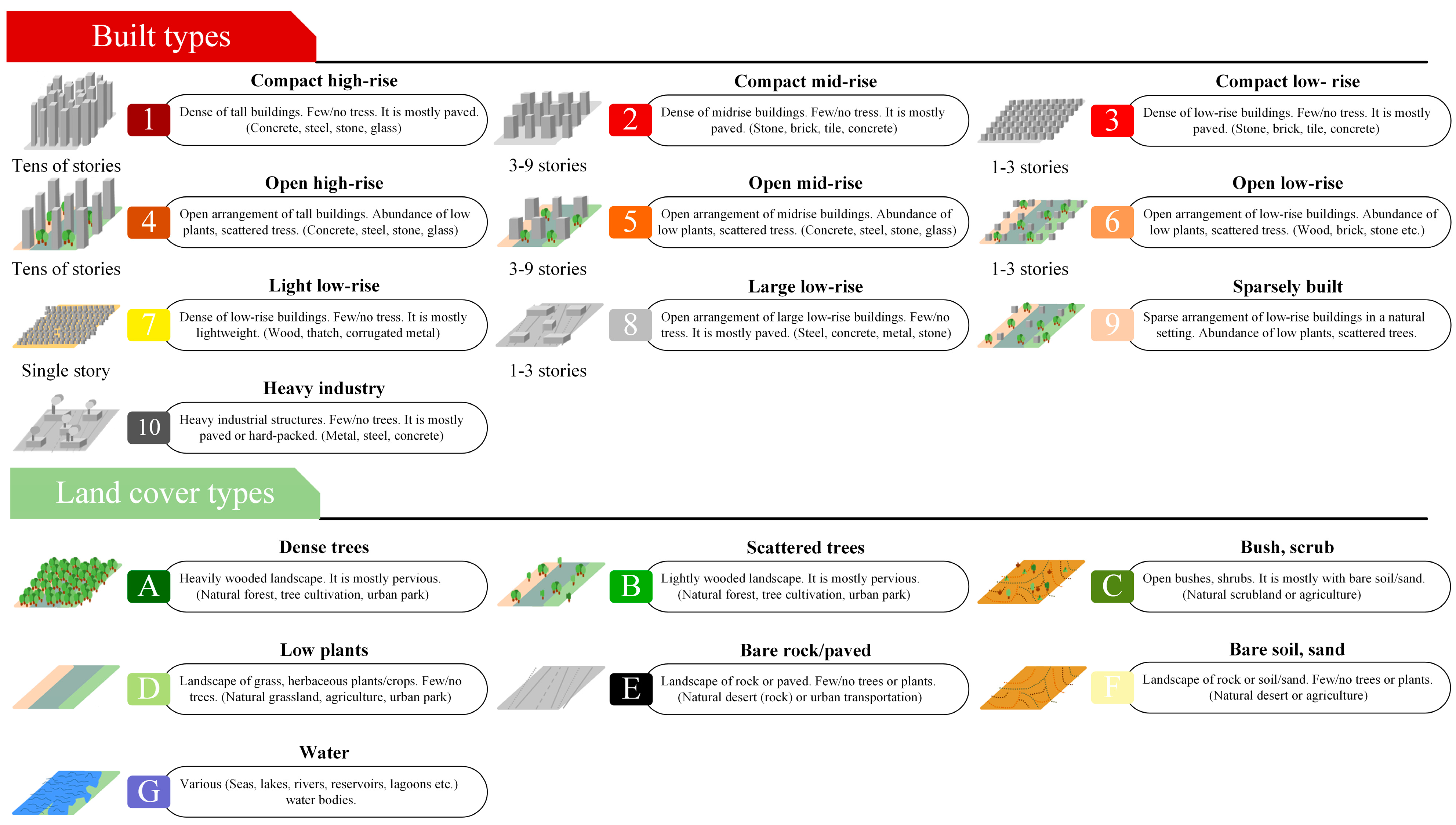
To fill the gap in the urban classification framework, Stewart and Oke proposed the local climate zones (LCZs) scheme in 2012 [9], which divided the areas of interest into 17 standard LCZ types including 10 built types and 7 land cover types, describing diverse urban landscapes ranging from hundreds of meters to several kilometers. The detailed information on each LCZ type is shown in Figure 1. Considering building height, spatial distribution and covering material of land surface structure, the system provides a standard evaluation framework for UHI studies. With the popularity of LCZ research in related fields, the demands for high-quality LCZ maps are also gradually increasing. However, until now, a variety of mapping quality assessments indicate that there is still a lot of room for improvement in LCZ mapping, which can only be improved when considering all built classes together or using weights defined by the morphological and climatic similarity of certain classes [10].
Geographic information system (GIS) based mapping shows high potential in producing high-quality LCZ maps [12], but large-scale GIS-based mapping is limited by data and complexity of operations, making RS-based mapping the mainstream. Most RS-based mapping products use pixels as mapping units, among which the Level 0 product mapping process proposed by the WUDAPT (The World Urban Database and Access Portal Tools) project is the most popular [13]. The WUDAPT method uses free Landsat image and SAGA GIS software to resample remote sensing images to 100 m and realize LCZ mapping through random forest. Until now, LCZ maps for more than 100 cities around the world have been completed and shared. However, WUDAPT-based LCZ maps clearly show a disadvantage in accuracy. Overall accuracy (OA) of the 90 LCZs uploaded on the WUDAPT portal is 74.5%, and the average OA of the built LCZ types of the 90 LCZs is only 59.3%, leaving much room for improvement [14]. To obtain high-quality LCZ maps, many researchers have made efforts in mapping methods. Verdonck used derived spectral information to help classification [15], while Liu and Shi proposed new network architecture for LCZ classification [16]. However, pixel-based classification still has two problems: (1) it cannot provide good boundaries for LCZ types; (2) most LCZ products are made with low resolution, resulting in mixed pixels.
Object-based classification has made great success in the field of high-resolution image analysis. In recent years, some scholars have begun to explore the application of object-based LCZ mapping. Collins and Dronova generated an object-based LCZ map for the urban areas of Salt Lake City, United States of America [17]. They argued that the object-based LCZ classification paradigm could better describe the boundaries of LCZ types. In addition, Ma et al. proved the effectiveness of object-based LCZ mapping through land surface temperature analysis of three cities in China [18]. Although the exploration of OBIA in the field of LCZ mapping has been gradually carried out, their research did not show the advantages of object-based LCZ mapping. If the object-based LCZ mapping is more advantageous, there is still no definite conclusion in existing research. In addition, many studies use auxiliary data to help LCZ mapping at present, which can be divided into two categories: (1) Derivation of related features. This method uses spectral index, mean, maximum, and minimum to aid classification [14]. (2) Addition of datasets. This approach uses multiple datasets simultaneously, such as Landsat, Sentinel, Global Urban Footprint, and Open Street Map [19,20]. Although multi-source data were used in their studies, the mapping units are all pixels, limiting the effectiveness of multi-source data.
The comparison between the object-based method and pixel-based method has been carried out in various fields. Shi and Liu compared two methods for mapping quasi-circular vegetation patches and recommended the object-based SVM approach to map the QVPs [21]. Nachappa proved that the object-based geon approach creates meaningful regional units and performs better than the pixel-based approach in landslide susceptibility mapping [22]. For land use/land cover (LULC) mapping and change detection, similar research was conducted, and the object-based method showed greater potential compared with the pixel-based method [23,24,25]. However, little research has systematically compared object-based and pixel-based methods in the field of LCZ mapping, especially with multi-source data. Since most LCZ products are made through the pixel-based paradigm, it is important to figure out the advantages and disadvantages of an object-based paradigm and whether image objects can maximize the benefits of multi-source data.
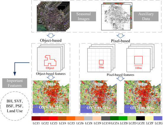
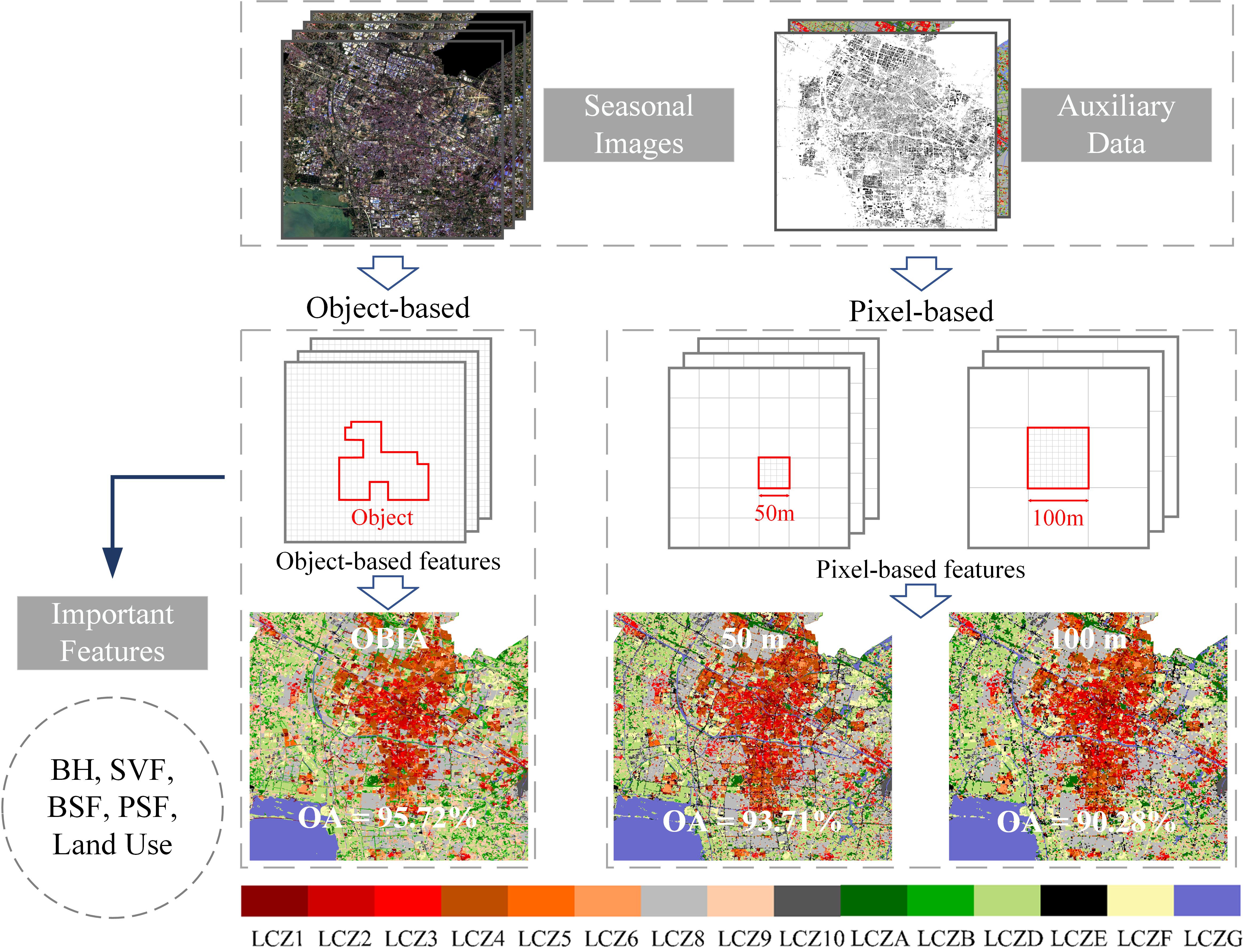
This study aims to systematically compare the object-based and pixel-based data with multi-source data. Since few studies have been carried out on object-based LCZ mapping, we further propose an improved object-based LCZ mapping workflow. The objects of this research are to: (1) complete the object-based LCZ mapping process with multi-source data and object-based sampling strategy; (2) compare the LCZ maps generated from two different types of paradigms; (3) assess multi-source features in the object-based LCZ mapping; (4) discuss the future direction for improving the object-based LCZ mapping.

2. Study Area and Multi-Source Data for LCZ Mapping

2.1. Study Area

This study is conducted in Changzhou, a city in Jiangsu Province, China, with longitude 119°08′–120°12′ east and latitude 31°09′–32°04′ north, which is shown in Figure 2. Changzhou is located on the southern bank of the lower reaches of the Yangtze River, the Taihu Lake Basin water network plain, in the southern part of Jiangsu Province. The terrain of the territory is slightly higher in the southwest and lower in the northeast, with a height difference of about 2 m. The climate of Changzhou is a subtropical monsoon climate, characterized by warm winters and cool summers. Changzhou has distinct seasonal characteristics and scarcely suffers from large-area and long-term cloud cover or snowfall, becoming an appropriate city for LCZ mapping research. The area investigated in this study covers approximately 800 km2, which comprises the main urban area and nearby rural area. As the number of LCZ classes varies from city to city because of the different urban form, 15 classes (nine built types and six land cover types) were taken into consideration in our study area.

2.2. Multi-Source Data Acquirement

Three types of data were used for mapping in this study: satellite images in raster format, building data and land use data in vector format. Sentinel-2 (S2) images of four seasons were used for data composition, which is introduced in Section 3.1. Six multispectral bands of S2 images were used in this study: B2, B3, B4 and B8 with 10 m Ground Sampling Distance (GSD) and B11 and B12 with 20 m GSD. The use of multi-season remote-sensing data has been shown to improve the accuracy of LCZ classification [19]. So seasonal S2 images are used and the related information is displayed in Table 1. Building data and land use data are used in this study to provide urban morphological information, common in GIS-based mapping [12]. Land use data include eight categories: water, low vegetation, woodland, bare soil, road, industrial area, residential area, and other facilities. These two types of data were obtained from Baidu Map and the local department, respectively, representing the study area in 2019.

3. Methods

For LCZ mapping, four main steps were conducted in this study (Figure 3):
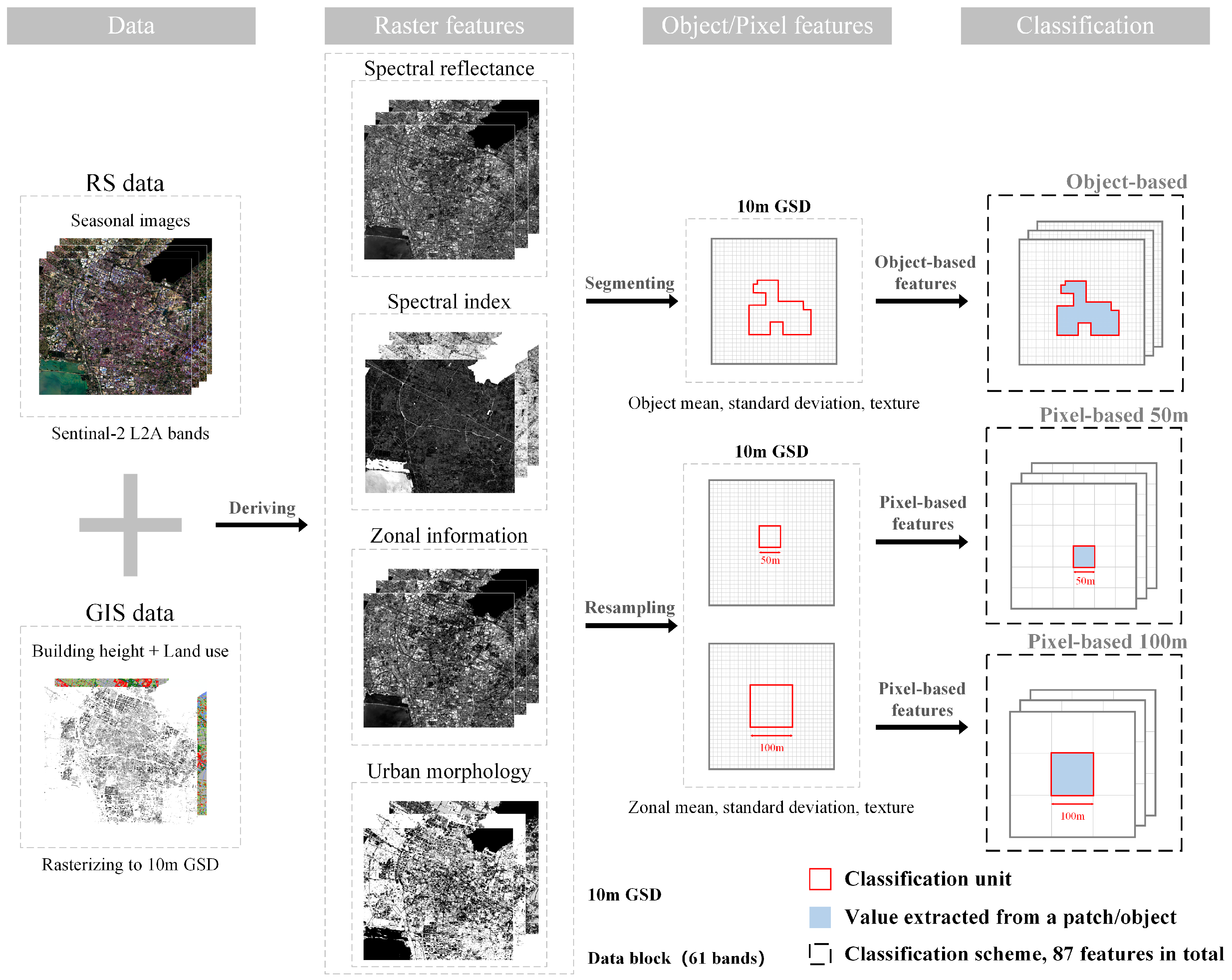
  • Data preprocessing. To obtain high-quality data for LCZ mapping. Seasonal composite satellite images were obtained as basic mapping data, while building data and land use data were converted to raster form. All data are resampled into 10 m GSD.
  • Feature derivation for LCZ mapping. For ricing spectral information and better depicting the urban form, diverse features were selected and derived, including spectral reflectance, spectral indices, zonal information obtained through filtering, urban morphological parameters (UMPs) that depict urban morphology.
  • Feature extraction based on image objects and patches. After obtaining segmentation results by multi-resolution segmentation (MRS) and determining the resampling size, we extracted zonal mean, standard deviation and texture from objects and pixels based on a 10 m data block respectively.
  • LCZ classification. LCZ samples based on objects or pixels were input to the random forest classifier for training and testing. Finally, each object or pixel was predicted by the random forest classifier for producing the LCZ map.

3.1. Data Preprocessing

Synthetic seasonal cloudless S2 images, rasterized building data and land use data were obtained to integrate RS and GIS information. For S2 images, after geometric correction and atmospheric correction from Google Earth Engine, a series of image preprocessing operations were carried out to make sure to obtain images without cloud. The QA60 band, which is a bitmask band with cloud mask information, was used to remove the pixels with cloud. Subsequently, image sets of each season were created by a date filter for the study areas and were then used to generate synthetic images based on the median of individual pixels. Finally, synthetic multi-season S2 images including B2, B3, B4, B8, B11 and B12 with 10 m were created for LCZ mapping with bilinear resampling method. GIS data were converted and resampled into 10 m. Building layer was assigned based on height while land use layer was assigned based on categories with values 0–7.

3.2. Derived Raster Features for LCZ Mapping

In this study, diverse features were extracted and stacked as a multi-channel data block with a resolution of 10 m. This data block includes spectral reflectance layers, spectral indices layers, zonal information layers in four seasons and UMPs including BH, SVF, BSF, PSF and land use layers. More information is shown in Table 2. The whole data block serves as the input for object-based and pixel-based methods to ensure that they are completely consistent for comparison. The input features in this data block are:
Spectral reflectance: blue (B2), green (B3), red (B4) and near-infrared (B8) were selected to provide spectral information. Considering that seasonal images were used in our study, 16 layers were finally obtained.
Spectral index: NDVI (Normalized Difference Vegetation Index), NDBI (Normalized Difference Built Index), NBAI (Normalized built-in Area Index), BRBA (Band Ratio for built-up Area), BSI (bare-soil Index) and MNDWI (Modified Normalized Difference Water Index) were used for rich spectral information. These spectral indices were demonstrated to be able to characterize vegetation, buildings, water and bare soil [26,27], aiding the classifier to mine underlying spectral differences and connections among diverse LCZ types. Notably, as the classification for built LCZ types is harder, three building-related spectral indices were selected for improving the performance of the classifier. Considering four seasons, a total of 24 spectral index layers were obtained.
Zonal information: Verdonck proved that using zonal information can effectively improve LCZ mapping quality on a fine scale [15]. In this study, we used a mean filter to obtain zonal information based on seasonal images. In detail, the filter is defined with size 11*11 and moving with step = 1. When the filter is at the edge of the image, the extent of the processing is outside the image; thus, zero-padding was applied. Finally, we obtained 16 layers containing zonal information.
Urban morphological parameter: Stewart and Oke defined LCZs with measurable and stable physical properties including SVF, Aspect Ratio (AR), BSF, Impervious Surface Fraction (ISF), PSF, Height of Roughness Elements and Terrain Roughness Class [9]. In this study, BH, SVF, BSF, and PSF were calculated, while the land use layer was obtained by assigning the value of every pixel according to the category, because they are available from our data and are widely used for LCZ mapping [12,28,29]. SVF is defined as the visible proportion of the sky hemisphere from a ground point [30]. Figure 4 displays the visible sky (S_sky) and the invisible sky (S_obstacle), which are determined by search radius (R) and building distribution. In this study, the SVF value for each pixel was obtained by SAGA GIS [31]. Building height data with 10 m GSD were input, and R was determined as 100 m. The relevant calculation formulas are displayed in Table 3.

3.3. Classification Schemes for LCZ Mapping

3.3.1. Object-Based Classification

MRS in Trimble eCognition software was used in this study, which adopts a bottom-up method to gradually merge homogeneous pixels into one object and determines the threshold of an object by parameters such as scale, color/shape, smoothness/tightness [32,33]. In addition to traditional LULC classification tasks, MRS has been successfully adopted in the field of urban functional zones mapping [34,35], which demonstrated that MRS has the potential for classifying diverse landscapes. Thus, MRS was selected for image segmentation in this study.
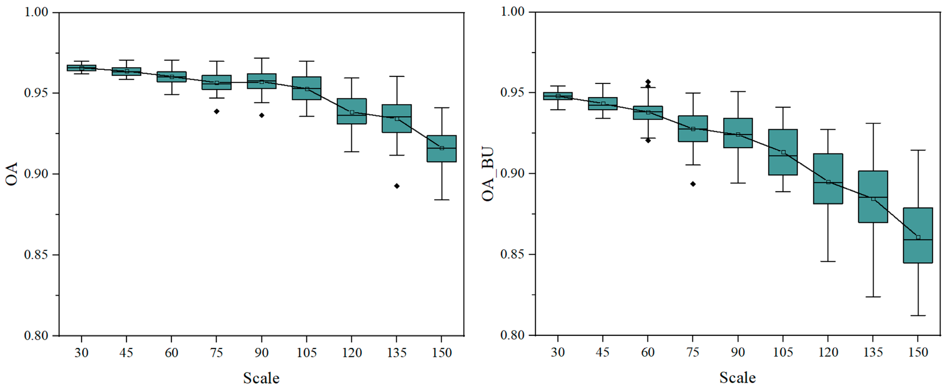
Regarding parameter settings, segmentation weights of spectral layers (16 layers) were set as 1 while others were set as 0. Segmentation parameters of color/shape and smoothness/compactness were considered as 0.9/0.1 and 0.5/0.5. A total of nine scales ranging from 30 to 150 were selected to evaluate mapping results in different scale scenarios.
For LCZ mapping, it has become well known that values extracted from an adjacent region (mean, standard deviation, maximum, minimum, et.) help classification [20]. However, most researchers used a moving window to calculate statistical values as a new feature map. In the object-based method, we extracted features from image objects. Three types of features were obtained through Trimble eCongnition for our classifier: mean, standard deviation and texture. The total number of features is 87. The number of features for each type is shown in Table 4.
The total number of mean features is 63. Sixty-one of them were calculated one by one from the layers we input. The remaining two features were MAX.DIFF and brightness. The total number of standard deviation features is 16, which were calculated from the composite S2 images. Gray Level Co-occurrence Matrix (GLGM) was used to extract texture features from the composite S2 images, which describes the distribution of co-occurring values of an image in a given area and provides a statistical view of the texture based on the image histogram. We selected eight features, including contrast, dissimilarity, homogeneity, angular second moment, entropy, mean, standard deviation and correlation with all angles.

3.3.2. Pixel-Based Classification

In pixel-based classification, two schemes with 50 and 100 m were designed for LCZ mapping. Although the most appropriate mapping scale for LCZ classification has not reached a consensus yet, Bechtel et al. argued that a “valid” LCZ may vary depending on the resolution, and mapping with 100–150 m is a good compromise while 10–30 m is too high [13]. Furthermore, the WUDAPT project, which strongly promotes the development of LCZ research, produced LCZ maps in a resolution of 100 m, leading most scholars to achieve LCZ classification in a resolution of 100 m [10,14,16,36]. Thus, 100 m was selected in this study as the first choice. In addition, since multi-source data can provide detailed urban information, making LCZ mapping possible at a fine scale. We selected 50 m as the second choice, which is almost the highest resolution in the LCZ mapping research [37]. Thus, after the optimal scale was selected for the object-based method, we compared the object-based method with the pixel-based method in 50 and 100 m.
In order to make the pixel-based method and the object-based method comparable, zonal mean, standard deviation and texture were extracted from image patches for LCZ classification instead of traditional resampled values. Similar to the object-based method, a total of 87 features were finally adopted: 63 of them were zonal mean calculated from the data block, 16 were standard deviation features, and 8 were texture features calculated from the composite S2 images.

3.4. Random Forest Classifier

Random forest has been widely adopted in the remote sensing field, showing great performance in classification and regression tasks [38,39,40]. By producing independent trees with randomly selected subsets through bootstrapping from training samples and input variables, the classifier obtains the final result through votes of majority trees. In addition, due to the popularity of the WUDAPT project, which achieves LCZ classification through random forest, most of the current LCZ maps were produced by random forest. We selected the same classifier to better exhibit the difference between object-based and pixel-based methods.
Since random forest is composed of independent decision trees, it is a machine learning algorithm that is sensitive to the different input features, which is convenient for us to analyze feature importance in the LCZ mapping field. Finally, the classifier we used in this study consists of 476 trees. In addition, 60% of the total sample data was selected for training the classifier, and all samples were used for testing, as we performed an area-based accuracy assessment for the object-based method.

3.5. Sampling Strategy

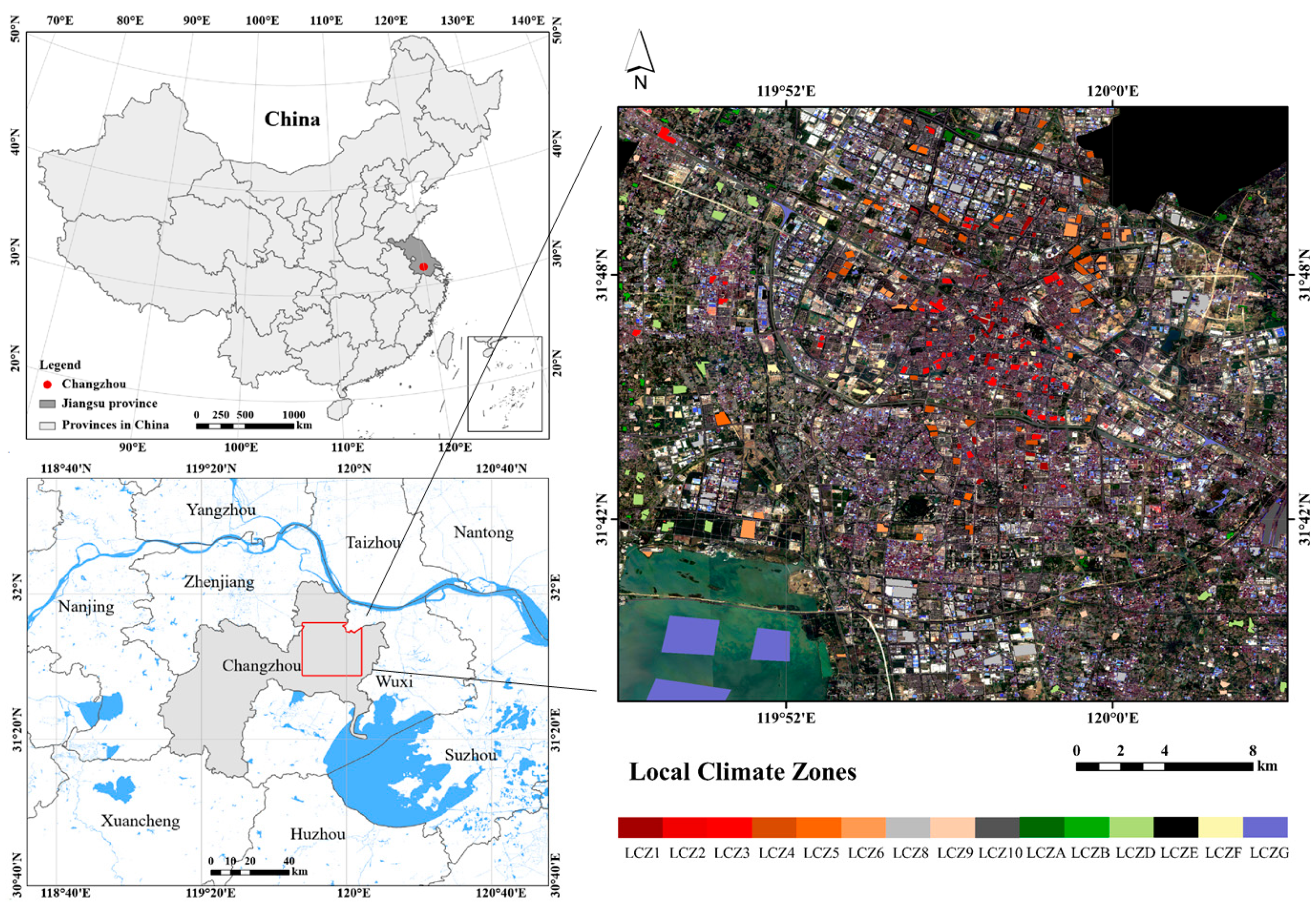
Three steps were conducted for sampling in our study. First, the sample polygons were digitalized on Google Earth software. Second, we stacked the samples with the segmentation/resampled layer and finally extracted reference objects/pixels. Considering the actual condition of Changzhou, we adopted 15 LCZ types including nine built types (excluding LCZ7) and six land cover types (excluding LCZC). Figure 5 displays the difference between object-based workflow and pixel-based workflow in sampling. Notably, when digitalizing on Google Earth, sampling criteria from Zhu et al. were conducted to identify diverse LCZ types [41]. In particular, for built LCZ types, after determining the target area uniform, a large area was distinguished as LCZ8 or LCZ10 while others were distinguished by height, compactness and material according to Figure 1.
Since the polygon samples obtained at the digitalization stage cannot completely coincide with the segmented image objects, it is hard to label objects correctly. Radoux set different overlay ratio thresholds for labeling different land cover categories, fully considering the differences among ground objects [42]. In addition, LCZ classification is gradually regarded as a scene classification task, and many scholars attempted to utilize surrounding information of samples to improve the robustness of the classifier [14,16,35]. For a similar purpose, diverse overlay ratios were set for each LCZ type. Taking 0.5 as a basic threshold (too high is meaningless while too low may introduce wrong samples), we adjusted the overlay ratio according to the complexity of an LCZ. Namely, simple scenarios require a higher threshold while complex ones need a lower threshold. Table 5 displays the settings we used. Finally, the stratified random sampling strategy was used to select training and test samples.

3.6. Accuracy Assessment

Overall accuracy ( OA ), kappa coefficient ( Kappa ), user’s accuracy, producer’s accuracy and F1-Score ( F 1 ) were used for accuracy assessment. Several accuracy metrics proposed for LCZ mapping including OA B U , OA N and WA were also taken into consideration [43]. The related formulas are shown in Table 6. For the object-based method, an area-based accuracy assessment was performed counting for the correct proportions of classified areas in segmented objects [44]. For the pixel-based method, all metrics were calculated by counting the correct number of pixels. In the accuracy metrics we designed, user’s accuracy and producer’s accuracy, which reflect commission error and omission error, were performed with a normalized confusion matrix. F1-score can be regarded as a harmonic average of model accuracy for better assessing per-class performance. OA B U is the OA on only the built types, and OA N is the OA of the built versus natural LCZ classes only. WA is a metric that accounts for similarity and dissimilarity between classes.

4. Results

4.1. Classifications of Object-Based Method in Multi-Scale Scenarios

4.1.1. Visual Interpretation Analysis of LCZ maps at Various Scales

To the best of our knowledge, no detailed assessment for object-based LCZ mapping has been made in state-of-the-art research. To assess the optimal scale of the object-based method, first, we conducted a visual interpretation analysis to evaluate LCZ maps in multi-scale scenarios.
Figure 6 shows LCZ mapping results as scale range from 30 to 150. In general, all maps show no obvious misclassifications because segmentation merges discrete pixels before classification. Analyzing each map individually, the maps at scales 30 and 45 were finer, and major roads were successfully classified into LCZEs. At scales 60–105, the fragmentation of the classification was reduced but still maintained a high agreement with the LCZ maps at scales 30 and 45. When the scale was greater than 105, the classification of urban areas changed greatly. From observation, the maps with scales 30–105 performed better, as they were relatively stable. At scales 120–150, the area of LCZ1-LCZ6 types increased, and the area of LCZ8 decreased. Although Bechtel et al. pointed out that LCZ types may vary with scale [13], our maps should not show much difference because they were trained with the same samples. In order to further analyze the results of each scale, we carried out precision analysis.

4.1.2. Accuracy Analysis in Multi-Scale Scenarios

Table 7 presents accuracy metrics for the object-based method with a scale ranging from 30 to 150. All results in Table 7 represent the average value of 50 runs. In general, all object-based classifications achieved over 85% accuracy for all accuracy metrics, especially WA and OA N , which surpassed 98% at all scales. This could be explained that in the object-based method, the classifier benefits from segmentation and avoids huge mistakes while the resampling process leads to mixed pixels (e.g., The classifier cannot distinguish objects between nature type and built type). As the segmentation scale became larger, all metrics decreased except for WA and OA N , which both peaked at scale 90, indicating the optimal scale required for natural and built types differs. The phenomenon of accuracy decrease was mainly in OA , Kappa and OA B U . As the scale surpassed 105, accuracy loss was accelerated in OA , Kappa and OA B U , which indicates that large scale is not suitable for built-type classification.
In particular, Figure 7 shows the variation of OA and OA B U to scale. OA was relatively stable at scale 30–90, and the mean curve formed a platform. When the scale is greater than 105, OA declines significantly, mainly at scales 105–120 and 135–150, where the slope of the curve is much higher, indicating that a large scale is not suitable for LCZ mapping. Considering that the object size increases as the scale increases, the decrease in accuracy may be caused by the fact that important classification features, such as BH and SVF, are blurred by the excessively large object. Although the variation curve of OA B U is similar to OA , the decline is more obvious than OA , indicating that the accuracy decrease is mainly in the built types. Both figures show a trend of variance increasing with the increasing scale, which can be attributed to two reasons: one is the feature uncertainty caused by large objects, and the other is the insufficient generalization ability due to the reduction of samples. In general, the mapping results are relatively stable at the scale of 30–90, indicating that the object-based method can be capable of LCZ mapping despite under-segmentation cases. In order to minimize the computational demands of mapping, we chose scale 90 as the optimal scale.

4.2. Comparison of Object-Based and Pixel-Based Methods

4.2.1. Overall Accuracy and Statistical Analysis Comparison

According to the results above, we chose scale 90 as our optimal parameter for the object-based method and compared the object-based method with the pixel-based method of 50 and 100 m. Table 8 displays related information of the three classification schemes, showing huge computational costs in the pixel-based methods.
Figure 8 displays the LCZ maps in three schemes. We can see that the object-based method provides better boundaries for LCZs, improving the visualization of the LCZ map. Table 9 displays the accuracy metrics of three classification schemes. All results were obtained from 50 classification repeats. In general, all metrics revealed that the object-based method performed better than the two pixel-based methods. In three classification schemes, all WA and OA N surpassed 97%, much higher than other accuracy metrics. With multi-source data, the pixel-based method performed better in 50 m instead of 100 m, which indicates that features in this study are able to characterize LCZs well at a fine scale. OA and kappa of the object-based method were both about 2% higher than those in the 50 m pixel-based method, while OA B U was only about 1% higher. Variances are displayed in Table 9. Two pixel-based methods exhibit smaller accuracy variances compared with the object-based method. We think that it can be attributed to more samples in the pixel-based methods.
To prove that there is a significant difference in accuracies between the object-based method and the pixel-based method, Student’s t-test was conducted to compare the means of OA of three schemes. In our study, independent samples t-test was conducted. Furthermore, to ensure that our test was statistically effective, Shapiro–Wilk test was conducted to test whether our data obey a normal distribution and all three sets of data passed the test with p value > 0.05. Levene’s test is conducted to test the equality of variances. All tests are finished with α = 0.05. Every set of data has 50 samples.
Table 10 displays the results of statistical tests. Levene’s tests both rejected null hypotheses, which means the data from the object-based method have different variances with two pairs of data from the pixel-based method under the condition α = 0.05. Under the premise of uneven variances, t-tests were conducted, and the results showed significant differences. Through statistical tests, we proved that the object-based method performed better than two pixel-based methods.

4.2.2. Per-Class Accuracy Comparison between Schemes

User’s accuracy and producer’s accuracy were used to assess errors of commission and omission. Each confusion matrix in Figure 9 was an accumulation of normalized confusion matrices (50-runs classification) where the original elements have been divided by the row total, ensuring that we can evaluate the object-based and the pixel-based method equally.
In two pixel-based methods, there was a significant similarity between the two matrices, but the results from 50 m performed better. By adding various features, the classifier can reach high accuracy in the high-resolution scenario. By comparing the object-based method with the pixel-based method in 50 m, the results indicated some differences between the two methods. The distribution of errors of commission and omission in the object-based method was more concentrated, while more non-zero values were scattered in the matrix in the 50 m scenario. In addition, the object-based method performed better in typical LCZ types such as LCZ4, LCZF, which always appear with distinct visual features. However, in some types such as LCZ2, LCZ5 and LCZ6, the object-based method performed worse. This failure indicates that complex scenes are still challenging for the object-based method. However, object-based results were trained with fewer samples, which limited the potential of the method.
It is not objective to evaluate the performance of a certain LCZ type with user’s accuracy or producer’s accuracy only. For instance, in Figure 8, all methods achieved a high producer’s accuracy with LCZD but with a lower user’s accuracy. Thus, for F1-Score, a comprehensive metric was selected to describe the performance of each LCZ type.
Figure 10 displays the performance of each LCZ type in the three schemes. Comparing two pixel-based schemes, the accuracy of each LCZ type increases, which indicates that adding multi-source features can help the classifier learn better in high-resolution cases. The results in the object-based method performed quite differently. Compared with the pixel-based method in 50 m, the variances of most LCZ types of the object-based method are larger. This is because the object-based method was trained with fewer samples. However, the object-based method performed much better on nature types and competitive results in built types despite LCZ2, LCZ5 and LCZ6. Considering that there is a much smaller number of samples in the object-based method, the object-based method showed great potential in LCZ mapping. In addition, according to our analysis above, the accuracy of built types can be improved at a fine scale.

4.3. Feature Importance Analysis Based on the Object-Based LCZ Classification

Random forest has been proven to be a classifier less affected by sample imbalance [45] and has more obvious advantages in improving mapping results with input features compared with deep learning methods [46]. Therefore, feature analysis based on random forest is meaningful. CFS is a relatively stable method in feature selection and it can maintain the effect of a classifier to a large extent [44]. In this study, CFS was used for feature selection, and the frequency of feature selection was used as a metric to assess feature importance.
Figure 11 shows the results of feature selection from scales 30 to 150 with 50 classification repeats at each scale. It can be seen from Figure 10 that the features selected by the object-based method mainly focus on four aspects: first, the urban morphological parameters related to LCZ definition: SVF, BSF, PSF, land Use, BH; second, the spectral indices that can represent characteristics of buildings, vegetation or water: NDBI, NBAI, MNDWI, BRBA; third, the spectral reflectance (including variation) standard deviation layers and convolution layers; finally, texture features.
Urban morphological parameters have high selectivity at each scale, which proves the importance of urban morphological parameters for LCZ classification. The spectral indices selected by CFS were mainly the bands containing short-wave infrared information, such as NDBI, NBAI and BRBA, indicating that short-wave infrared information is also important for LCZ mapping. NDVI did not stand out from many features, which is inconsistent with the conclusion of Qiu [19]. The reason is that PSF is similar to NDVI while PSF can better depict regional permeable surface information. From the selection of spectral features, we can see the uniqueness of LCZ classification. Feature selection focused on convolutional features (including zonal information) and standard deviation features, indicating that LCZ classification pays more attention to the spectral information of a local area rather than to a single pixel. As the scale increases, the selection of convolutional features gradually disperses, indicating that with the increase in mixed objects, the spectral features of objects become more chaotic and meaningless. Meanwhile, the selection of texture features gradually highlights as the scale increases, indicating that as the object grows, the texture features inside the object become more obvious and no longer appear redundant. In addition, features of each season were selected, indicating that time series features help classification.

5. Discussion

Currently, LCZ mapping is mostly divided into two streams: RS based and GIS based. LCZ mapping based on the integration of the two methods is considered to have great potential, and a few studies have begun to focus on the integration of the two [35]. The methods used in this study can be regarded as an integration of the two mapping methods, which further proves the great potential of the integrated framework.
From the perspective of the mapping accuracy, mapping results of small-scale/high-resolution were still higher than all other cases, which is inconsistent with some studies showing that mapping with moderate scale/resolution is better [13,16]. This is mainly because all features adopted in this study have regional information to help mapping reflect the mean or standard deviation value of image objects. Verdonck obtained a similar conclusion to ours and obtained the optimal mapping result by utilizing neighborhood information features [15]. However, an LCZ represents a region spanning at least hundreds of meters, which means that mapping at a too small scale will cause the result to deviate from the application purpose. Thus, it is not encouraged to map at a too small scale. In addition, the amount of computation brought by the small scale is huge, which is more obvious in the pixel-based method.
According to accuracy results and statistical analysis, object-based methods show advantages and are stable at multiple scales, which is because the boundaries offered the by object-based method reduce confusion among LCZs. In the pixel-based method, it is difficult for regular grids to correctly divide LCZ boundaries, making classification difficult. Object-based methods are not beneficial to all LCZ types. For example, segmentation makes labeling and classification of LCZ5 types more difficult. Segmentation makes various features separated, which is an urgent problem to be solved when applying the object-based method to LCZ mapping. Lehner and Blaschke proposed the use of object-based methods for urban structure type mapping [47]. If it is applied to LCZ mapping, the potential of object-based LCZ mapping may be further explored.
In feature analysis, the maximum difference, convolution features, NDBI, BRBA, BH, BSF, PSF, and land use were frequently selected, indicating that the above features are extremely important in LCZ mapping. Among the features of remote sensing data, convolution features that contain neighborhood information and the two spectral indices that contain short-wave infrared information performed well. These features have also been adopted in previous studies and are proven to be effective [20]. Mapping based on GIS data has always been considered as a method of high-precision LCZ mapping [12]; we also demonstrate the validity of GIS data.
The performance of the machine learning classifier is closely related to the number of training samples [44]. Considering that the number of training samples will decrease as the scale parameter increases, the mapping accuracies of multiple scales were similar to the object-based methods. In the case of similar mapping accuracy, the choice of scale should be determined by the application conditions. Misclassification is acceptable in some cases because similar LCZ types represent similar temperature conditions. However, if the 17 LCZ types cannot meet application requirements and if the mapping scale is small, an LCZ subclass can be considered to be added. Kotharkar solved the confusing LCZ types problem by employing 21 LCZ types [48]. Perera also pointed out that using LCZ subclasses is necessary for further analysis of urban development status [49].

6. Conclusions

This study describes an attempt to compare the object-based method and the pixel-based method for LCZ mapping with multi-source data, aiming to determine a more advantageous mapping paradigm. In addition, four types of features were derived for ensuring mapping quality: (1) composite seasonal satellite images; (2) diverse spectral indices; (3) zonal information; (4) urban morphological information.
In multiple scale cases, the object-based method performed stable unless in under-segmentation cases. When the scale was less than 90, the OA and OA B U of all maps exceeded 95.5% and 92%, respectively, and no significant difference behaved in visual performance. When the scale was larger than 105, the object-based method showed an obvious performance decline, especially in built types, which indicated that multi-source data cannot provide sufficient urban information with under-segmentation.
Comparing the object-based method with a pixel-based method in 50 and 100 m, the object-based method showed the best performance and statistical difference from pixel-based methods (p < 0.05). OA , OA B U , OA N and WA of the object-based method increased by about 2%, 1%, 1% and 1%, respectively, compared with the 50 m case (the better one) while 10 times the amount of data was processed in the pixel-based method. In per-class analysis, the object-based method showed a significant advantage in the natural types and competitive performance in built types, while partial LCZ types such as LCZ2, LCZ5, and LCZ6 performed worse than the pixel-based method in 50 m. However, we found that built type accuracy can be improved with finer segmentation.
In feature analysis, CFS was selected to evaluate the importance of features, and frequency characterized feature importance. For urban morphological information, BH, SVF, BSF, PSF and land use exhibited an extremely high frequency of selection at all scales. Among other features, convolutional layers, BRBA, NBDI, NBAI, MNDWI of certain seasons performed well, while original image bands were hardly selected, indicating that derived spectral features can better characterize differences among LCZs.
In our study, the object-based method can achieve equivalent mapping results with less computation cost compared with the pixel-based method, making it more suitable for large-scale mapping. In the future, the object-based method will become more advantageous when the segmentation results of urban regions can be improved.

Author Contributions

Conceptualization, L.M.; Data curation, Z.Y., L.M., L.Z. and G.H.; Formal analysis, Z.Y., L.Z. and G.H.; Funding acquisition, L.M.; Investigation, Z.Y. and L.M.; Methodology, Z.Y., L.M. and W.H.; Project administration, L.M.; Resources, L.M.; Software, L.M. and W.H.; Supervision, L.M., H.L. and G.L.; Validation, Z.Y., H.L. and G.L.; Visualization, Z.Y.; Writing—original draft, Z.Y.; Writing—review & editing, Z.Y., L.M., L.Z., H.L. and G.L. All authors have read and agreed to the published version of the manuscript.

Funding

This research was funded by National Natural Science Foundation of China, grant number 42171304 and 41701374.

Data Availability Statement

Sentinel 2 images are openly available on Google Earth Engine. Building data is available on request from the authors. Land use data is not available due to the legal restrictions.

Acknowledgments

This work was supported by the funding provided by the National Natural Science Foundation of China (42171304, 41701374), and the Fundamental Research Funds for the Central Universities. Sincere thanks to the anonymous reviewers and members of the editorial team for the comments and contributions.

Conflicts of Interest

The authors declare no conflict of interest.

References

  1. Tadros, W.; Wellenstein, S.N.; Das, A. Demographic Trends and Urbanization (English); World Bank Group: Washington, DC, USA, 2021. [Google Scholar]
  2. Giridharan, R.; Ganesan, S.; Lau, S.S.Y. Daytime urban heat island effect in high-rise and high-density residential developments in Hong Kong. Energy Build. 2004, 36, 525–534. [Google Scholar] [CrossRef]
  3. Rizwan, A.M.; Dennis, L.Y.; Chunho, L.I.U. A review on the generation, determination and mitigation of Urban Heat Island. J. Environ. Sci. 2008, 20, 120–128. [Google Scholar] [CrossRef]
  4. Yadav, N.; Yadav, N.; Sharma, C.; Peshin, S.K.; Masiwal, R. Study of intra-city urban heat island intensity and its influence on atmospheric chemistry and energy consumption in Delhi. Sustain. Cities Soc. 2017, 32, 202–211. [Google Scholar] [CrossRef]
  5. Grimmond, S. Urbanization and Global Environmental Change: Local Effects of Urban Warming. Geogr. J. 2007, 173, 83–88. [Google Scholar] [CrossRef]
  6. Chen, J.; Chen, J.; Liao, A.; Cao, X.; Chen, L.; Chen, X.; Mills, J. Global land cover mapping at 30m resolution: A POK-based operational approach. ISPRS J. Photogramm. Remote Sens. 2015, 103, 7–27. [Google Scholar] [CrossRef] [Green Version]
  7. Liu, Y.; Fang, X.; Xu, Y.; Liu, Y.; Fang, X.; Xu, Y.; Zhang, S.; Luan, Q. Assessment of surface urban heat island across China’s three main urban agglomerations. Theor. Appl. Climatol. 2018, 133, 473–488. [Google Scholar] [CrossRef]
  8. Mathew, A.; Khandelwal, S.; Kaul, N. Investigating spatio-temporal surface urban heat island growth over Jaipur city using geospatial techniques. Sustain. Cities Soc. 2018, 40, 484–500. [Google Scholar] [CrossRef]
  9. Oke, T.R.; Stewart, I.D. Local Climate Zones for Urban Temperature Studies. Bulletin of the American Meteorol. Soc. 2012, 93, 1879–1900. [Google Scholar]
  10. Bechtel, B.; Alexander, P.J.; Beck, C.; Böhner, J.; Brousse, O.; Ching, J.; Xu, Y. Generating WUDAPT Level 0 data–Current status of production and evaluation. Urban Clim. 2019, 27, 24–45. [Google Scholar] [CrossRef] [Green Version]
  11. Zhou, L.; Ma, L.; Johnson, B.A.; Yan, Z.; Li, F.; Li, M. Patch-Based Local Climate Zones Mapping and Population Distribution Pattern in Provincial Capital Cities of China. ISPRS Int. J. Geo-Inf. 2022, 11, 420. [Google Scholar] [CrossRef]
  12. Quan, S.J.; Bansal, P. A systematic review of GIS-based local climate zone mapping studies. Build. Environ. 2021, 196, 107791. [Google Scholar] [CrossRef]
  13. Bechtel, B.; Alexander, P.J.; Böhner, J.; Ching, J.; Conrad, O.; Feddema, J.; Stewart, I. Mapping Local Climate Zones for a Worldwide Database of the Form and Function of Cities. ISPRS Int. J. Geo-Inf. 2015, 4, 199–219. [Google Scholar] [CrossRef] [Green Version]
  14. Yoo, C.; Han, D.; Im, J.; Bechtel, B. Comparison between convolutional neural networks and random forest for local climate zone classification in mega urban areas using Landsat images. ISPRS J. Photogramm. Remote Sens. 2019, 157, 155–170. [Google Scholar] [CrossRef]
  15. Verdonck, M.; Okujeni, A.; Linden, S.V.; Demuzere, M.; De Wulf, R.; Van Coillie, F. Influence of neighbourhood information on ‘Local Climate Zone’ mapping in heterogeneous cities. Int. J. Appl. Earth Obs. Geoinf. 2017, 62, 102–113. [Google Scholar] [CrossRef]
  16. Liu, S.; Shi, Q. Local climate zone mapping as remote sensing scene classification using deep learning: A case study of metropolitan China. ISPRS J. Photogramm. Remote Sens. 2020, 164, 229–242. [Google Scholar] [CrossRef]
  17. Collins, J.; Dronova, I. Urban Landscape Change Analysis Using Local Climate Zones and Object-Based Classification in the Salt Lake Metro Region, Utah, USA. Remote Sens. 2019, 11, 1615. [Google Scholar] [CrossRef] [Green Version]
  18. Ma, L.; Yang, Z.; Zhou, L.; Lu, H.; Yin, G. Local climate zones mapping using object-based image analysis and validation of its effectiveness through urban surface temperature analysis in China. Build. Environ. 2021, 206, 108348. [Google Scholar] [CrossRef]
  19. Qiu, C.; Schmitt, M.; Mou, L.; Ghamisi, P.; Zhu, X.X. Feature Importance Analysis for Local Climate Zone Classification Using a Residual Convolutional Neural Network with Multi-Source Datasets. Remote Sens. 2018, 10, 1572. [Google Scholar] [CrossRef] [Green Version]
  20. Yokoya, N.; Ghamisi, P.; Xia, J.; Sukhanov, S.; Heremans, R.; Tankoyeu, I.; Tuia, D. Open Data for Global Multimodal Land Use Classification: Outcome of the 2017 IEEE GRSS Data Fusion Contest. IEEE J. Sel. Top. Appl. Earth Obs. Remote Sens. 2018, 11, 1363–1377. [Google Scholar] [CrossRef] [Green Version]
  21. Shi, L.; Liu, Q.; Huang, C.; Li, H.; Liu, G. Comparing Pixel-Based Random Forest and the Object-Based Support Vector Machine Approaches to Map the Quasi-Circular Vegetation Patches Using Individual Seasonal Fused GF-1 Imagery. IEEE Access 2020, 8, 228955–228966. [Google Scholar] [CrossRef]
  22. Nachappa, G.T.; Kienberger, S.; Meena, S.R.; Hölbling, D.; Blaschke, T. Comparison and validation of per-pixel and object-based approaches for landslide susceptibility mapping. Geomat. Nat. Hazards Risk 2020, 11, 572–600. [Google Scholar] [CrossRef]
  23. Berhane, T.; Lane, C.; Wu, Q.; Anenkhonov, O.A.; Chepinoga, V.V.; Autrey, B.C.; Liu, H. Comparing Pixel- and Object-Based Approaches in Effectively Classifying Wetland-Dominated Landscapes. Remote Sens. 2018, 10, 46. [Google Scholar] [CrossRef] [PubMed] [Green Version]
  24. De Giglio, M.; Greggio, N.; Goffo, F.; Merloni, N.; Dubbini, M.; Barbarella, M. Comparison of Pixel- and Object-Based Classification Methods of Unmanned Aerial Vehicle Data Applied to Coastal Dune Vegetation Communities: Casal Borsetti Case Study. Remote Sens. 2019, 11, 1416. [Google Scholar] [CrossRef] [Green Version]
  25. Balha, A.; Mallick, J.; Pandey, S.; Gupta, S.; Singh, C.K. A comparative analysis of different pixel and object-based classification algorithms using multi-source high spatial resolution satellite data for LULC mapping. Earth Sci. Inform. 2021, 14, 2231–2247. [Google Scholar] [CrossRef]
  26. Pal, M.; Antil, K. Comparison of Landsat 8 and Sentinel 2 Data for Accurate Mapping of Built-up Area and Bare Soil. In Proceedings of the 38th Asian Conference on Remote Sensing, New Delhi, India, 23–27 October 2017. [Google Scholar]
  27. Bhatti, S.S.; Tripathi, N.K. Built-up area extraction using Landsat 8 OLI imagery. GIScience Remote Sens. 2014, 51, 445–467. [Google Scholar] [CrossRef] [Green Version]
  28. Zhou, Y.; Zhang, G.; Jiang, L.; Chen, X.; Xie, T.; Wei, Y.; Lun, F. Mapping local climate zones and their associated heat risk issues in Beijing: Based on open data. Sustain. Cities Soc. 2021, 74, 103174. [Google Scholar] [CrossRef]
  29. Zheng, Y.; Ren, C.; Xu, Y.; Wang, R.; Ho, J.; Lau, K.; Ng, E. GIS-based mapping of Local Climate Zone in the high-density city of Hong Kong. Urban Clim. 2018, 24, 419–448. [Google Scholar] [CrossRef]
  30. Hantzschel, J.; Goldberg, V.; Bernhofer, C. GIS-based regionalisation of radiation, temperature and coupling measures in complex terrain for low mountain ranges. Meteorol. Appl. 2005, 12, 33–42. [Google Scholar] [CrossRef]
  31. Conrad, O.; Bechtel, B.; Bock, M.; Dietrich, H.; Fischer, E.; Gerlitz, L.; Böhner, J. System for automated geoscientific analyses (SAGA) v. 2.1.4. Geosci. Model Dev. 2015, 8, 1991–2007. [Google Scholar] [CrossRef] [Green Version]
  32. Baatz, M.; Schape, A. Multiresolution Segmentation: An Optimization Approach for High Quality Multi-Scale Image Segmentation. Adv. Remote Sens. 2000, 5, 12–23. [Google Scholar]
  33. Benz, U.C.; Hofmann, P.; Willhauck, G.; Lingenfelder, I.; Heynen, M. Multi-resolution, object-oriented fuzzy analysis of remote sensing data for GIS-ready information. ISPRS J. Photogramm. Remote Sens. 2004, 58, 239–258. [Google Scholar] [CrossRef]
  34. Du, S.; Liu, B.; Zhang, X. Mapping large-scale and fine-grained urban functional zones from VHR images using a multi-scale semantic segmentation network and object based approach. Remote Sens. Environ. 2021, 261, 11248. [Google Scholar] [CrossRef]
  35. Zhou, W.; Ming, D.; Lv, X.; Zhou, K.; Bao, H.; Hong, Z. SO–CNN based urban functional zone fine division with VHR remote sensing image. Remote Sens. Environ. 2020, 236, 111458. [Google Scholar] [CrossRef]
  36. Kim, M.; Jeong, D.; Kim, Y. Local climate zone classification using a multi-scale, multi-level attention network. ISPRS J. Photogramm. Remote Sens. 2021, 181, 345–366. [Google Scholar] [CrossRef]
  37. Yoo, C.; Lee, Y.; Cho, D.; Im, J.; Han, D. Improving Local Climate Zone classification using incomplete building data and sentinel 2 images based on convolutional neural networks. Remote Sens. 2020, 12, 3552. [Google Scholar] [CrossRef]
  38. Breiman, L. Random forests. Mach. Learn. 2001, 45, 5–32. [Google Scholar] [CrossRef] [Green Version]
  39. Sim, S.; Im, J.; Park, S.; Park, H.; Ahn, M.H.; Chan, P.W. Icing detection over East Asia from geostationary satellite data using machine learning approaches. Remote Sens. 2018, 10, 631. [Google Scholar] [CrossRef] [Green Version]
  40. Richardson, H.J.; Hill, D.J.; Denesiuk, D.R.; Fraser, L.H. A comparison of geographic datasets and field measurements to model soil carbon using random forests and stepwise regressions (British Columbia, Canada). Gisci. Remote Sens. 2017, 54, 573–591. [Google Scholar] [CrossRef]
  41. Zhu, X.X.; Hu, J.; Qiu, C.; Shi, Y.; Kang, J.; Mou, L.; Wang, Y. So2Sat LCZ42: A benchmark data set for the classification of global local climate zones [Software and Data Sets]. IEEE Geosci. Remote Sens. Mag. 2020, 8, 76–89. [Google Scholar] [CrossRef] [Green Version]
  42. Radoux, J.; Bogaert, P. Accounting for the area of polygon sampling units for the prediction of primary accuracy assessment indices. Remote Sens. Environ. 2014, 142, 9–19. [Google Scholar] [CrossRef]
  43. Bechtel, B.; Demuzere, M.; Sismanidis, P.; Fenner, D.; Brousse, O.; Beck, C.; Verdonck, M.L. Quality of Crowdsourced Data on Urban Morphology—The Human Influence Experiment (HUMINEX). Urban Sci. 2017, 1, 15. [Google Scholar] [CrossRef] [Green Version]
  44. Ma, L.; Cheng, L.; Li, M.; Liu, Y.; Ma, X. Training set size, scale, and features in Geographic Object-Based Image Analysis of very high resolution unmanned aerial vehicle imagery. ISPRS J. Photogramm. Remote Sens. 2015, 102, 14–27. [Google Scholar] [CrossRef]
  45. Liu, T.; Abd-Elrahman, A.H.; Morton, J.; Wilhelm, V.L. Comparing fully convolutional networks, random forest, support vector machine, and patch-based deep convolutional neural networks for object-based wetland mapping using images from small unmanned aircraft system. GIScience Remote Sens. 2018, 55, 243–264. [Google Scholar] [CrossRef]
  46. Athiwaratkun, B.; Kang, K. Feature representation in convolutional neural networks. arXiv 2015, arXiv:1507.02313. [Google Scholar]
  47. Lehner, A.; Blaschke, T. A Generic Classification Scheme for Urban Structure Types. Remote Sens. 2019, 11, 173. [Google Scholar] [CrossRef] [Green Version]
  48. Kotharkar, R.; Bagade, A. Local Climate Zone classification for Indian cities: A case study of Nagpur. Urban Clim. 2018, 24, 369–392. [Google Scholar] [CrossRef]
  49. Perera, N.G.R.; Emmanuel, R. A “Local Climate Zone” based approach to urban planning in Colombo, Sri Lanka. Urban Clim. 2018, 23, 188–203. [Google Scholar] [CrossRef] [Green Version]
Figure 1. The LCZ system and related definitions from Stewart and Oke [9,11]. The contents in brackets are the common materials or landscapes for diverse LCZs.
Remotesensing 14 03744 g001
Figure 2. Study area and reference data sampled from Google Earth.
Remotesensing 14 03744 g002
Figure 3. The schematic workflow of LCZ mapping and comparison schemes.
Remotesensing 14 03744 g003
Figure 4. The calculation of SVF. SVF is the visible proportion of the sky hemisphere. S_sky and S_obstacle are the visible sky and invisible sky. The angle (θ) and the search radius (R) are determined by the highest building in the search range and users’ definition, respectively.
Remotesensing 14 03744 g004
Figure 5. The process of sampling and labeling. In step 1, different LCZ types were digitalized on Google Earth and the red block is an example of the original sample. In step 2, pixels overlaid by the original sample were labeled in a pixel-based process while image objects were labeled according to the overlay ratio we set. Step 3 displays the final samples for a pixel-based method and object method. The blue line and orange line represent the process of labeling objects and pixels respectively.
Remotesensing 14 03744 g005
Figure 6. LCZ maps in multi-scale scenarios.
Remotesensing 14 03744 g006
Figure 7. Accuracy boxplots from scale 30 to 150. The left picture shows the change in OA , and the right picture shows the change in OA B U .
Remotesensing 14 03744 g007
Figure 8. LCZ maps of three comparison schemes. (AC) are the enlarged display areas for object-based, pixel-based in 50 m and pixel-based 100 m respectively.
Remotesensing 14 03744 g008
Figure 9. Confusion matrices of three schemes. Each confusion matrix is the accumulation of 50 normalized confusion matrices where the original elements have been divided by the row total. (ac) are the confusion matrices of object-based, pixel-based in 50 m, pixel-based in 100 m respectively.
Remotesensing 14 03744 g009
Figure 10. F1-score boxplots of the three classification schemes. (ac) are the F1-scores of object-based, pixel-based in 50 m, pixel-based in 100 m respectively. The diamonds represent outliers. The horizontal line and the square in the box represent the median and mean of F1-scores for a set of data respectively. The number next to the box is the mean of F1-scores.
Remotesensing 14 03744 g010
Figure 11. Results of feature selection from scales 30 to 150 with 50 runs at each scale. All results were obtained through CFS. “1”, “2”, “3”, “4” represent blue, green, red, nir, respectively. “Con” represents the convolutional layer, “Std” represents the standard deviation layer, and the abbreviations for the four seasons are “Spr”, “Sum”, “Aut”, “Win”. Features with a total frequency of fewer than 20 times were not considered.
Remotesensing 14 03744 g011
Table 1. Remote sensing image data for data composition.
Satellite ImageSeasonDate
Sentinel-2 L2ASpring2020-03-01 to 2020-05-31
Summer2019-06-01 to 2019-08-31
Autumn2020-09-01 to 2020-11-30
Winter2020-12-01 to 2021-02-28
Table 2. Overview of features in the data block.
FeatureContentSeasonalNumber
Spectral reflectanceBlue, Green, Red, Nir16
Spectral indexNDVI, MNDWI, NDBI, NBAI, BSI, BRBA16
Zonal informationConvolutional layers24
UMPBH, SVF, BSF, PSF, Land Use 5
Table 3. Urban morphological parameters. In this study, the final UMPs for mapping were extracted from mapping units.
UMPDefinitionFormula
Building Height n is the number of buildings in a classification unit (a resampled pixel or an object); B S i is the area of one building; B H i is the height of one building; S s i t e is the area of a classification unit. BH = i = 1 n B S i × B H i S _ s i t e
Sky View Factor n is the number of pixels in a classification unit; S V F i is the S V F in pixel i ; S _ s k y i and S _ o b s t a c l e i are the area of visible sky and invisible sky for pixel i , respectively; S V F i = S _ s k y i S _ s k y i + S _ o b s t a c l e i   SVF = i = 1 n S V F i n
Building Surface Fraction n is the number of buildings in a classification unit. BSF = i = 1 n B S i S _ s i t e
Permeable Surface Fraction S _ p e r is the area of the permeable surface in a classification unit (average NDVI for four seasons > 0.2) PSF = S _ p e r S _ s i t e
Table 4. Summary of feature types for object/pixel-based classification.
FeatureNumber
Mean63
Standard deviation16
Texture8
Table 5. Overlay ratio settings for LCZs.
LCZ TypeOverlay RatioExplanation
LCZ10.55The composition of LCZ1 is complex, and the threshold should not be too high.
LCZ20.65The distribution of LCZ2 is relatively concentrated, and a higher threshold can be set.
LCZ30.60Same as LCZ2.
LCZ40.55LCZ4 is easier to distinguish, but because it contains a certain degree of vegetation, the threshold should not be too high.
LCZ50.55Same as LCZ4.
LCZ60.45LCZ6 is similar to LCZ5, but constructions are usually sparser, making a low threshold necessary.
LCZ80.60Most of them belong to industrial areas with concentrated distribution; thus, a higher threshold can be set.
LCZ90.45The natural coverage is greater than that of artificial buildings; thus, a low threshold is set.
LCZ100.65Same as LCZ8.
LCZA0.75LCZA is widely distributed and easy to identify, setting a high threshold.
LCZB0.50LCZB includes low vegetation and a few trees; thus, a low threshold is needed for labeling.
LCZD0.60Mostly cultivated land and grassland, covering a large area, including diverse vegetation, the threshold should not be too high or too low.
LCZE0.65LCZE is easy to identify but is small in area. A higher threshold is necessary.
LCZF0.60Same as LCZE.
LCZG0.75LCZG is widely distributed and easy to identify, setting a high threshold.
Table 6. Description of accuracy metrics.   N i c is the area/number of class i correctly classified, w is weight matrix introduced by Betchel [31].
MetricFormula
Overall Accuracy ( OA ) 1 N i = 1 n N i c
Built-up OA ( OA B U ) 1 N B u i l t i = 1 n N B u i l t , i c
Natural OA ( OA N ) 1 N N a t u r a l i = 1 n B u i l i t N N a t u r a l , i c
Weighted Accuracy ( WA ) 1 N i = 1 n N a t u r e w × N i c
F1-Score (F1) 2 ( P r e c i s i o n   ×   R e c a l l P r e c i s i o n   +   R e c a l l )
Table 7. Accuracy statistics from scale 30 to 150 with the average values from 50 runs.
Scale O A   % K a p p a   % O A B U   % O A N   % W A   %
3096.5996.0594.8199.5799.22
4596.3895.7894.3499.6499.22
6096.0595.3593.8399.6199.19
7595.6794.8492.8099.7199.18
9095.7294.8892.4399.7699.24
10595.2994.3891.3499.5799.09
12093.8492.6689.5299.0998.68
13593.4592.1888.4699.1098.63
15091.6490.1586.1098.9398.13
Table 8. Training and test samples of each scheme. The values in the table are the number of objects/pixels.
Units to Be ClassifiedTraining SamplesTest Samples
Object-based28,071560949
Pixel-based 50 m316,52211,52919,224
Pixel-based 100 m79,47637546267
Table 9. Accuracy assessment results for three schemes with the average values from 50 runs for each scheme.
O A   ( σ 2 )   % K a p p a   ( σ 2 )   % O A B U   ( σ 2 )   % O A N   ( σ 2 )   % W A   ( σ 2 )   %
Object-based95.72 (5.04 × 10⁻⁵)94.88 (7.2 × 10⁻⁵)92.43 (1.7 × 10⁻⁴)99.76 (2.31 × 10⁻⁵)99.24 (1.86 × 10⁻⁶)
Pixel-based 50 m93.71 (2.78 × 10⁻⁶)92.95 (3.5 × 10⁻⁶)91.60 (5.17 × 10⁻⁶)98.60 (6.57 × 10⁻⁷)98.23 (3.34 × 10⁻⁷)
Pixel-based 100 m90.28 (7.57 × 10⁻⁶)89.25 (9.28 × 10⁻⁶)88.11 (1.68 × 10⁻⁵)97.47 (3.49 × 10⁻⁶)97.01 (1.39 × 10⁻⁶)
Table 10. Results of statistical tests. The test results are the comparison results with the object-based method.
Levene’s TestIndependent Samples t-Test
p ValueSignificant Differencep ValueSignificant Difference
OBIA vs. 100 m pixel<0.001Yes<7 × 10−50Yes
OBIA vs. 50 m pixel<0.001Yes<4 × 10⁻²⁶Yes
Publisher’s Note: MDPI stays neutral with regard to jurisdictional claims in published maps and institutional affiliations.

