Article

NeXtNow: A Convolutional Deep Learning Model for the Prediction of Weather Radar Data for Nowcasting Purposes

by
Alexandra-Ioana Albu
1,†,
Gabriela Czibula
1,*,†,
Andrei Mihai
1,†,
Istvan Gergely Czibula
1,†,
Sorin Burcea
2 and
Abdelkader Mezghani
3
1
Department of Computer Science, Babeş-Bolyai University, 400084 Cluj-Napoca, Romania
2
Romanian National Meteorological Administration, 013686 Bucharest, Romania
3
Meteorologisk Instittut, 0371 Oslo, Norway
*
Author to whom correspondence should be addressed.
These authors contributed equally to this work.
Remote Sens. 2022, 14(16), 3890; https://0-doi-org.brum.beds.ac.uk/10.3390/rs14163890
Submission received: 4 July 2022 / Revised: 7 August 2022 / Accepted: 8 August 2022 / Published: 11 August 2022
(This article belongs to the Special Issue Artificial Intelligence-Based Learning Approaches for Remote Sensing)

Abstract

:
With the recent increase in the occurrence of severe weather phenomena, the development of accurate weather nowcasting is of paramount importance. Among the computational methods that are used to predict the evolution of weather, deep learning techniques offer a particularly appealing solution due to their capability for learning patterns from large amounts of data and their fast inference times. In this paper, we propose a convolutional network for weather forecasting that is based on radar product prediction. Our model (NeXtNow) adapts the ResNeXt architecture that has been proposed in the computer vision literature to solve the spatiotemporal prediction problem. NeXtNow consists of an encoder–decoder convolutional architecture, which maps radar measurements from the past onto radar measurements that are recorded in the future. The ResNeXt architecture was chosen as the basis for our network due to its flexibility, which allows for the design of models that can be customized for specific tasks by stacking multiple blocks of the same type. We validated our approach using radar data that were collected from the Romanian National Meteorological Administration (NMA) and the Norwegian Meteorological Institute (MET) and we empirically showed that the inclusion of multiple past radar measurements led to more accurate predictions further in the future. We also showed that NeXtNow could outperform XNow, which is a convolutional architecture that has previously been proposed for short-term radar data prediction and has a performance that is comparable to those of other similar approaches in the nowcasting literature. Compared to XNow, NeXtNow provided improvements to the critical success index that ranged from 1% to 17% and improvements to the root mean square error that ranged from 5% to 6%.

Graphical Abstract

1. Introduction

Short-term weather analysis and forecasting for the next 0 to 6 h, which is known as weather nowcasting [1,2], are of great interest in meteorology due to the increasing number of severe weather events that can severely affect the safety of the human population by causing damage and even mortality. For instance, precipitation nowcasting, which refers to the prediction of rainfall intensity in specific regions in the near future, plays an important role in our daily life [2] and represents a challenging topic in nowcasting. The problem is that short-term weather forecasting is complex and difficult, even for operational meteorologists, mainly due to the large volume of data that needs to be examined and interpreted in a short period of time. In addition, nowcasting [3] is highly dependent on various environmental conditions and requires a lot of human experience.
Significant progress has recently been made in the field of nowcasting, ranging from operational nowcasting systems to the numerous computational intelligence solutions that have been proposed in the literature for detecting the occurrence of severe weather events [4,5]. Radar data [6] are useful for nowcasting [7,8]. Most operational nowcasting systems use numerical weather prediction (NWP) models, which combine radar data and other meteorological observations to provide weather forecasts for up to 6 h in the future, e.g., the INCA system [9]. Still, there are a lot of challenges in issuing precise nowcasting warnings as most severe events (e.g., severe convective storms) occur within small spatial areas and have short overall life cycles. Despite the significant improvements that have been achieved by NWP models in precipitation nowcasting, there are still some limitations to their use, such as insufficient computational resources in operational centers and increased error rates at convection-permitting scales [10].
Most existing operational and semi-operational methods for nowcasting are based on cell-tracking algorithms that use radar data as inputs. A real-time cell-tracking algorithm named TITAN, which is useful for single cells, was introduced by Dixon and Wiener [7] and the SCIT system, which uses a more complex cell-tracking algorithm and reflectivity thresholds, was later proposed by Johnson et al. [8]. An operational nowcasting tool that uses a centroid cell-tracking method (named TRT) was also developed by Hering et al. [11] and used by Meteo Swiss, while Germany’s National Meteorological Service uses a nowcasting system that is called NowCastMIX, which was introduced by James et al. [5] and employs fuzzy logic rules to analyze remote and ground observations. Fuzzy logic is also used in a cell-tracking algorithm that was proposed by Jung and Lee [4]. AROME [12] is a prediction model that is used to provide a forecast for up to 30 h in the future and has been used by Meteo France since 2008, while AROME-NWC [13] was later developed for nowcasting in the range of 0–6 h.
Machine learning (ML) techniques are useful computational intelligence tools that can assist operational meteorologists in decision-making as they are able to learn relevant patterns from weather-related data. Deep learning (DL) [14,15] models have become popular within the ML domain as they are able to express target functions that are more complex than those that are encoded by traditional ML models. Additionally, DL models can automatically extract useful features from raw data, thereby removing the difficult task of manual feature engineering that is required by classical ML models. DL architectures are characterized by a hierarchy of multiple levels of representations. Despite the complex aspects of this type of neural model, the key advantage of DL models is the fact that they are universal approximators, i.e., they have the ability to learn arbitrary functions as a composition of several operations.
Reflectivity (R) and Doppler radial velocity (V) are radar products that are used by operational meteorologists to monitor the spatiotemporal evolution of precipitating clouds and thus, they are useful in weather nowcasting.
These reflectivity and velocity values are also used by operational radar algorithms to estimate rainfall and to track and classify storms: R values that are higher than 35 dBZ [7,16] suggest the possible occurrence of convective storms, which are associated with heavy rainfall. The prediction of the values of these radar products based on their historical measurements is important for the early assessment of storm evolution, which can lead to improved nowcasting and timely severe weather warnings.
Time series data, which represent the values of the selected variables at specific time points, are generally used in forecasting because of the temporal characteristics of these data. This study used time series radar data to predict the values of the radar products in a specific geographical region, based on their historical values. The contribution of the paper is twofold. Firstly, the proposal of NeXtNow, which is a new convolutional weather forecasting model that was adapted from the ResNeXt [17] architecture that has been proposed in the computer vision literature for the task of spatiotemporal prediction. Our proposed model has an encoder–decoder architecture that consists of ResNeXt blocks and simple convolutions, which maps past radar measurements onto radar measurements that are recorded in the future. Therefore, NeXtNow is a customized version of ResNeXt for the short-term prediction of radar data. We opted for the convolutional architecture instead of a recurrent alternative due to its training and inference efficiency. The ResNeXt architecture was chosen due to the versatility of ResNet-type [18] architectures, which allows for the design of models that can be customized for specific tasks by stacking multiple blocks of the same type. Moreover, we empirically showed that the inclusion of multiple past radar measurements led to more accurate predictions further in the future. The performance of our proposed NeXtNow model was evaluated using two case studies, which consisted of real radar data that were collected from the Romanian National Meteorological Administration (NMA) and the Norwegian Meteorological Institute (MET). The obtained results were analyzed from a meteorological perspective to examine the ability of the NeXtNow model to capture relevant patterns in the evolution of radar echoes, i.e., patterns that could be relevant for nowcasting severe weather phenomena. Comparisons between NeXtNow and other models in the literature highlighted that NeXtNow outperformed a convolutional architecture [19] that was proposed for short-term radar data prediction and that its performance was also comparable to the performances of other similar approaches from the nowcasting literature. To the best of our knowledge, an approach that is similar to NeXtNow has not yet been proposed in the nowcasting literature.
To summarize, the following research questions guided this study:
RQ1
How can the ResNeXt deep learning architecture be adapted for the task of spatiotemporal prediction and customized for the short-term prediction of radar data? (This led to the development of the NeXtNow model.)
RQ2
How does the NeXtNow model perform using real radar data? Would adding multiple past radar measurements improve the future prediction performance?
RQ3
Does the ResNeXt model improve the performance of the short-term prediction of radar data? Is the performance improvement that is achieved by NeXtNow statistically significant from similar existing approaches?
The rest of the paper is organized as follows. Section 2 presents a literature review of recent machine learning and deep learning approaches for weather nowcasting that use radar data (Section 2.1) and an overview of the case studies that were used to evaluate our proposed model (Section 2.2). The methodology that was used in our work is detailed in Section 2.3. Section 3 presents the experimental evaluation of our proposed approach and the comparisons to similar models are presented in Section 4. The last section presents the conclusions of this study and potential directions for future research.

2. Materials and Methods

2.1. Recent Literature Advances in Nowcasting, Based on Radar Data Prediction

Various classical ML and DL models have been introduced in the literature for weather nowcasting. In the following section, we summarize the nowcasting techniques that are based on radar data that have been proposed recently.
Prudden et al. [20] reviewed the existing forecasting methods for precipitation prediction that are based on radar data and the machine learning techniques that are applicable for radar-based precipitation nowcasting. Four classes of methods for precipitation nowcasting were mentioned by the authors: persistence-based methods, probabilistic and stochastic methods, nowcasting convective development and ML-based approaches. The study emphasized the performance improvements that could be obtained by applying deep neural networks combined with domain knowledge about the physical system that was being modeled. The authors also highlighted the potential of generative adversarial networks, which are able to capture data uncertainty and generate new data that follow the same distribution patterns as the input data.
Han et al. [21] used support vector machines (SVMs) for radar data nowcasting, which was modeled as a binary classification task. The model was trained to identify whether the radar would detect a radar echo >35 dBZ in the following 30 min. The features that characterized the input data included temporal and spatial information. The experiments revealed a probability of detection (POD) of around 0.61, a critical success index (CSI) of 0.36 and a false alarm rate (FAR) of about 0.52.
Ji [22] employed artificial neural networks for short-term precipitation prediction using radar observations that were collected from China from 2010 to 2012. The reflectivity values were extracted from the raw data, then interpolated into 3D data and used to train the predictive model. The minimum and maximum values that were obtained for the root mean square error (RMSE) were 0.97 and 4.7, respectively [22].
A convolutional neural network (CNN) model was proposed by Han et al. [16] for predicting convective storms in the near future using radar data. The model was designed as a binary classification model to predict whether radar echo values would be higher than 35 dBZ in the next 30 min. The input radar data were represented by 3D images and the output was also a 3D image, in which each point of the image was "1" when the radar echo was predicted to be higher than 35 dBZ in the next 30 min and "0" when it was not. The experiments produced a CSI value of 0.44.
Socaci et al. [19] proposed an adaptation of the Xception deep learning model, which they named X N o w , for the short-term prediction of radar data. Experiments were performed using radar data that were provided by the Romanian National Meteorological Administration and an average normalized root mean square error of less than 3% was obtained.
The U-Net convolutional architecture has been employed in multiple studies on weather nowcasting using radar data [23,24]. Agrawal et al. [23] proposed a U-Net model for precipitation nowcasting. Their proposed model surpassed several baselines of other methods in terms of short-term prediction (up to 1 h), namely the persistence model and an optical flow algorithm, as well as the high-resolution rapid refresh (HRRR) system, but was outperformed by the HRRR model in terms of forecasts for up to 5 h. The RainNet model, which was proposed by Ayzel et al. [25], is a U-Net model that was trained using a logcosh objective function. Trebing et al. [24] introduced a lightweight U-Net model that used depth-wise separable convolutions. Their model achieved a similar performance to that of the classical U-Net while only having a quarter of its parameters.
Ciurlionis and Lukosevicius [26] used a CNN model to forecast future precipitation using current precipitation data. They used precipitation data that were estimated using a radar and trained the model with four time steps as the inputs and the next step as the output (i.e., when t was the current step, the input data were t 3 , t 2 , t 1 and t and the model predicted data for t + 1 ). To predict further in the future, they used consecutive predictions (using the predicted data from the previous step as the input for the next step). They compared their approach to four basic numerical algorithms: the persistence model, a basic translation algorithm, a step translation algorithm and a sequence translation algorithm. They measured whether the models correctly predicted zero or non-zero values (i.e., they transformed the task into a classification problem). When predicting one time step, both the CNN and the sequence translation algorithm had a CSI of 0.81, while the others had CSI values of under 0.8. For predictions further in the future, the CNN had a better performance than the sequence translation algorithm; for example, at 60 min, the CNN model had a CSI of 0.71 while the numerical algorithm had a CSI of 0.65.
Differentiating from the general trend of using deep learning for machine learning models, Mao and Sorteberg [27] proposed a model that was based on a random forest (RF) for precipitation nowcasting. The random forest was trained to predict precipitation data. The inputs for the model were multiple types of data, with the main ones being precipitation data that were estimated using a radar, AROME numerical model predictions and other various data from ground weather stations, such as air pressure, air temperature and/or wind speed. To evaluate the model, the predictions were transformed into two classes: below 0.1 and above or equal to 0.1. They obtained a CSI of 0.49 for the proposed model, while the automatic radar nowcasting had a CSI of 0.42 and a baseline numerical model had a CSI of 0.33.
Bonnet et al. [28] used a video prediction model named PredRNN++, which was based on ConvLSTM combined with gradient highway units (GHUs), to predict radar reflectivity and had radar reflectivity as the input. They only used the reflectivity from the lowest elevation angle, which was collected every 5 min. The input data consisted of 10 time steps and the model predicted 10 time steps into the future. In order to measure the performance of the model, they also transformed the predictions into classifications using the thresholds of 10 dBZ for predictions and 20 dBZ for observations. In terms of metrics, they used CSI and the equitable threat score (ETS), which is an improvement on CSI that also takes true negatives into consideration. Their model obtained a CSI of 0.52 and an ETS of 0.46 for prediction at 15 min and outperformed ENCAST, which is the model that is currently used in São Paulo, Brazil, based on the extrapolation of the data that were collected from the radar.
While the majority of nowcasting models that have been proposed so far have been based on a single machine learning model, Xiang et al. [29] proposed a model that combined two types of neural networks in order to improve the nowcasting results: decision trees and numerical methods. The goal of their model was to predict the amount of precipitation at a single point 1–2 h in the future (they targeted points where there were weather stations so they were able to compare the predictions to the ground truth values that were obtained by the stations). The dataset was processed so it only contained time steps with meteorological activity. Their model worked in three steps: first, they used a numerical model for trajectory tracking to compute the trajectory of the meteorological phenomenon (e.g., storm, clouds, etc.); then, there was a feature extraction phase, in which the best features were selected (some were just general features that were provided by the weather station and some were dependent on the previous phase, such as cropping images depending on the computed trajectory); the final phase consisted of using three models to separately predict the amount of precipitation. Each model used a different set of features from the features that were extracted in the second phase. For the final output, these three values were summed up with different weights. They tested the model using different features that were extracted in the second phase. The best results were 4.035 for the RMSE and 246.52 for the mean absolute percentage error (MAPE).
One of the main problems with using convolutional neural networks that were trained with conventional loss functions to predict images is that the predictions tend to be blurry or smoothed out. Hu et al. [30] proposed an improvement for nowcasting models by adding generative adversarial networks (GANs) as a second step after the usual predictive model. They proposed two types of GANs: a spatial GAN (acting on the actual image) and a spectral GAN (acting on the spectrum of the image following a fast Fourier transform). A masked-style loss function was introduced to improve the sharpness of the generated images. In addition, a new metric (the power spectral density score (PSDS)) was proposed, which was computed based on the spectrum of the images. In order to evaluate the quality of the predictions, another metric (the learned perceptual image patch similarity (LPIPS)) was used, which was measured according to the perceptual similarity between the observations and the predictions. The CSI metric was employed to measure the performance of the model using binarized values. In their experiments, U-Net and ConvLSTM were used as base models. The results that were obtained using both types of GANs were better than those that were obtained using only the spatial GAN, except when measuring CSI at the lowest threshold. Adding the mask-style loss yielded better results in most cases. As mentioned before, the original models yielded better results than the GANs for CSI at the lowest threshold, but this changed at higher thresholds. The GANs produced better LPIPS scores, which were even better when using the mask-style loss function (0.412 for the original ConvLSTM and 0.27 for the ConvLSM with both GANs and the loss function). The PSDS scores were significantly improved when using the GANs and the loss function (0.78 for the original ConvLSTM and 0.16 for the ConvLSTM with both GANs and the loss function).
Choi and Kim [31] also used GANs to improve the performance of U-Net models. Their goal was to predict radar reflectivity using radar reflectivity as the input data. The authors proposed a precipitation nowcasting model (Rad-cGAN) that was based on a conditional generative adversarial network (cGAN). To evaluate their model, they compared their estimated precipitation values using the ZR model to the observed ground truth precipitation values that were gathered at several dams. They obtained a Pearson correlation coefficient of 0.86, an RMSE of 0.42, a Nash–Sutcliffe efficiency (NSE) of 0.73 and a CSI of 0.81.

2.2. Case Studies

In the following section, we describe the case studies that were used to evaluate the proposed NeXtNow model. The two case studies were conducted using datasets from Romania (provided by the NMA) and Norway (provided by the MET), which were selected because they belonged to different geographical/climatic areas and contained different radar measurements (as further highlighted in Table 1), thus allowing us to test the performance of the NeXtNow model more thoroughly.

2.2.1. First Case Study (NMA Data)

The NMA dataset that was used in our first case study was collected by a Doppler single-polarization radar that is located in central Romania. During a full volume scan, which is completed every 6 min, the radar outputs many different products that are related to the location, intensity and movement of precipitating clouds and their associated meteorological phenomena. For the experiments, we used the base reflectivity (R) product and the base velocity (V) product. The radar collects these base products at nine elevation angles, effectively gathering nine sets of velocity and reflectivity data at each time step. For both products, we used the data from the lowest four elevation angles, which resulted in eight products in total: R01, R02, R03, R04, V01, V02, V03 and V04. The reflectivity and Doppler radial velocity were used for the NMA case study as these are the first products that are analyzed by forecasters to identify weather features. The use of velocity fields can be theoretically useful because they can introduce the effects of convergence zones into the model for the prediction of the initiation and evolution of convective storms. The experiments that are presented in Section 3 empirically sustained this hypothesis.
To train, validate and test the model, 20 summer days with heavy rain, wind and hail and without any meteorological events were extracted from the observations, which corresponded to events that were observed in June 2010 (2nd, 10th, 12th, 13th, 14th, 19th, 20th, 22nd, 23rd and 24th), June 2017 (from 3rd to 7th) and June 2018 (11th, 13th, 15th, 16th and 21st). The study area was the central Romania region (central Transylvania) as the radar is located near the village of Bobohalma. The month of June was selected for the NMA case study as, in Romania, it is the month that the most convective storms and convective systems develop in the Carpathian basin. The dataset included days both with and without severe meteorological events and thus, a diverse dataset was obtained. Out of the entire area that is scanned by the radar, we focused on a central square with a size of 256 × 256 cells (the radar is located in the middle of this square).

2.2.2. Second Case Study (MET Data)

The MET radar dataset that was used in our second case study consisted of composite reflectivity values that were obtained from the MET Norway Thredds Data Server [32]. The data, which are available at [33], were obtained by processing the raw reflectivity measurements that were retrieved from multiple radars. Thus, the reflectivity product that is stored at the MET Norway is a composite map that is obtained from all elevations and tilts by taking into account the radar scans that have the best quality and not the strongest reflectivity across the elevations. This composite reflectivity product is obtained by applying an interpolation procedure and using different weights for the various radars, depending on their quality and other meteorological or non-meteorological factors that can alter the radar measurements. The reflectivity values that were used in our experiments were collected at intervals of 5 min.
To train, validate and test the model, days with and without meteorological events were selected from December 2020 (23rd, 25th, 26th and 27th), January 2021 (17th and 18th), March 2021 (3rd and 4th), April 2021 (12th and 13th), June 2021 (the entire month) and January 2022 (1st–25th). The days were selected so as to obtain a diverse dataset that contained days both with and without severe meteorological events and included both summer and winter months. The analyzed geographical area was a region surrounding Oslo. From the entire map, a square of 256 × 256 pixels was selected.
Table 1 describes the datasets that were used in our case studies. The second column in the table indicates the radar products of interest and the last column shows the number of days on which the radar data that were used in each case study were collected.

2.3. Methodology

With the goal of answering our first research question (RQ1), we developed and evaluated our NeXtNow deep learning model, which was customized for the short-term prediction of weather radar products. NeXtNow was adapted for radar data prediction from the ResNeXt [17] architecture, which is mainly used for image processing. To the best of our knowledge, no other architecture that is based on ResNeXt has been proposed for weather nowcasting or spatiotemporal prediction problems. While several works have proposed fully convolutional or convolutional–recurrent neural networks for weather forecasting, they have employed simple and causal 2D or 3D convolutional architectures [34] and architectures that were inspired by U-Net [24] or the Xception model [19]. The basic details of the ResNeXt deep learning model are presented in Section 2.3.1, then Section 2.3.2 introduces the model that was used in our approach. Our NeXtNow learning model is introduced in Section 2.3.3, while the testing stage of NeXtNow and the methodology that was employed for the performance evaluation is discussed in Section 2.3.4.

2.3.1. ResNeXt Architecture

The ResNeXt architecture was proposed by Xie et al. [17] as an improved version of the R e s N e t model [35]. The R e s N e t architecture [35] addresses the difficulty in training very deep neural networks by introducing shortcut connections, a technique in which the input of an architectural block is added to its output in order to obtain the final output. By passing information from earlier layers to deeper layers, the network can optimize residual mappings, thus making it possible to efficiently train very deep architectures. This process can be viewed as a form of feature fusion, in which features at different levels of depth are combined using an addition operation [36]. Multiple residual blocks are stacked to form deep networks [35].
ResNeXt further builds on this architectural blueprint by using grouped convolutions instead of plain convolutions inside the residual blocks. Grouped convolutions are a type of convolutional layer in which the input is split channel-wise into multiple groups, with each group being processed individually by convolutions and concatenated at the end to obtain the final result. This construction has been shown to be equivalent to applying a set of aggregated transformations, which can be formalized as follows.
Given an input x and a hyperparameter that is called cardinality C, an aggregated transformation can be obtained from a set of transformations { τ 1 , , τ C } as:
F ( x ) = i = 1 C τ i ( x )
Following the strategy in R e s N e t , the aggregated transformation is a residual connection, which leads to the following computation for the output:
y = x + i = 1 C τ i ( x )
Figure 1 shows a schematic representation of the two types of blocks that are used in the R e s N e t and ResNeXt architectures. It has been shown experimentally that tuning the hyperparameter C can lead to significant performance improvements in image classification tasks [17].
As in the case of R e s N e t , the ResNeXt architecture is composed of a succession of blocks [17].

2.3.2. Formalization, Data Modeling and Preprocessing

We denoted the radar products of interest by P = { r 1 , r 2 , , r n } , where n is the dimensionality of P (the number of radar products that were used). For our case studies that were described in Section 2.2, we obtained the following values for P and n:
  • For the first case study (NMA dataset), n = 8 and P = { R 01 , R 02 , R 03 , R 04 , V 01 , V 02 , V 03 , V 04 } ;
  • For the second case study (MET dataset), n = 1 and P = { C R } .
The radar data that were input at a certain time moment t were denoted by I t and were modeled as 3D images with n channels (corresponding to the available radar products), with the i-th channel representing the value of the radar product r i at time t. More specifically, the OX and OY axes represented the longitudinal and latitudinal values of the geographical area and the OZ axis represented the channels (i.e., the values of the radar products P at time moment t).
A sample 4-channel 3D image (with n = 4 products) is shown in Figure 2.
Given a certain step k, the goal of our learning problem was to predict the 3D image at time moment t from the 3D images that were collected at the time moments t k , t k + 1 , , t 1 . In our model, the output was also an n-channel 3D image, in which the value of a point on the i-th channel of the image I t was the value that was predicted for the radar product r i at time t. We noted that one time step (i.e., the time period between two consecutive time moments t 1 and t) represented the time resolution between two consecutive radar scans. More specifically, a time step was 6 min for the NMA case study and 5 min for the MET case study.
We denoted the sequence of 3D images that represented the radar data that were collected at time moments t k , t k + 1 , , t 1 by S e q ( t , k ) = < I t k , I t k + 1 , , I t 1 > . In this context, the target function of our learning problem was a function M that mapped the k-length sequence of n-channel 3D images ( S e q ( t , k ) ) onto another n-channel 3D image ( I t ), i.e., I t = M ( S e q ( t , k ) ) . The NeXtNow deep learning model learned hypothesis h, which was an approximation of M ( h M ), i.e., h ( I t k , I t k + 1 , , I t 1 ) I t t . Thus, for a sequence of images ( S e q ( t , k ) ), NeXtNow provided a multi-channel 3D image I t that contained the estimation of the values of the radar products at time t.
A sequence of 3D images that contained radar data that were collected at different time moments t was available. A dataset D was created from sequences in the form of < I t k , I t k + 1 , , I t 1 > , i.e., a sequence of n-channel 3D images that represented radar data that were collected at time moments t k , t k + 1 , , t 1 . For each instance, the S e q ( t , k ) from the ground truth D (i.e., the n-channel 3D image I t that contained the values of the radar products at time t) was available and was used to train the model.
Before building the NeXtNow deep learning model, a preprocessing step was applied to the 3D images I t to correct any possible errors that existed in the radar data. For the NMA dataset, two different preprocessing methods were used, depending on the product. For R, the only preprocessing that was carried out was to replace the “No Data” (NaN) values with “0”. For the V product, there was a more complex preprocessing step. The issue with V was that it was a very noisy product because it represented the velocity relative to the radar, so there were some cases in which the radar could not properly estimate the direction or the speed, thus producing invalid values. These invalid values appeared often enough that they could interfere with the model learning [37]. We addressed this problem by introducing a cleaning step, which replaced the invalid values with valid values. The new values were computed as the weighted average of the values in the neighborhood surrounding the invalid value. The weight of a value in the neighborhood was inverse proportional to the difference between that value and the invalid value.
The raw MET data were preprocessed as follows. Since the raw data had negative reflectivity values, which were not important for nowcasting, these values were all replaced with a constant value of −1. Additionally, the NaN values that corresponded to missing radar measurements were replaced with values that were outside the domain of valid reflectivity values, i.e., −5, in order to be able to distinguish them from the negative values and the reflectivity values that were of interest (i.e., the positive values).
As well as the previous preprocessing steps, the data were normalized using the classical min-max normalization method. For the min-max normalization, we used the minimum and maximum values from the domain of the radar products instead of the minimum and maximum values from the training dataset. This way, we made sure that the same values in different datasets were assigned the same normalized values. In the case of the MET dataset, the minimum value that was used for normalization was −5, which corresponded to the missing radar measurements.

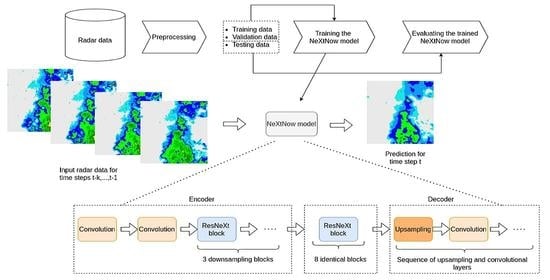
2.3.3. Building the NeXtNow Model

The predictive model NeXtNow was built using a training dataset that consisted of training samples in the form of ( S e q ( T , k ) , I t ), where I t = M ( S e q ( T , k ) ) represented the ground truth (the 3D image that consisted of the real values of the radar products at time t) that was used to train the instance S e q ( t , k ) = < I t k , I t k + 1 , , I t 1 > .
The proposed model had a fully convolutional encoder–decoder architecture, which was formed of three main components. The first component was an encoder, which was inspired by the ResNeXt architecture.
The encoder consisted of two classical convolutions, which had the role of providing multiple feature maps for the inputs, followed by three ResNeXt blocks. The blocks were constructed according to the original ResNeXt paper [17], as presented in Section 2.3.1. The final convolution in the block multiplied the filter size by four, while the group convolution downsampled the input image by a factor of two. Each convolution in the block was followed by a batch normalization layer and the ReLU activation function. The convolutions that were used in the encoder had a kernel size of 3 × 3.
The second component was a series of eight identical ResNeXt blocks, with 1024 filters each. In contrast to the blocks that were used in the encoder, the blocks that were included in this component did not change the resolution or number of filters of their inputs, but they did have the aim of obtaining refined representations for the feature maps that were retrieved from the encoder. Empirically, we found that the addition of these additional blocks was beneficial to the model’s overall performance.
While the first two components benefited from the use of ResNeXt blocks, we opted for a succession of simple convolutional layers for the decoder as experimenting with more complex architectural components did not lead to a better performance for the forecasting model. Therefore, in our proposed model, the decoder consisted of a series of upsampling layers, followed by convolutions. Following a standard approach to designing architectures for image-to-image tasks, the number of filters was progressively increased in the encoder and decreased in the decoder.
A schematic representation of the N e X t N o w architecture is shown in Figure 3.
The proposed architecture represented a new purely convolutional approach to weather nowcasting. The main advantage of our model was the simplicity and flexibility of the architecture, which allowed it to be easily adapted for other spatiotemporal prediction tasks with few hyperparameters that needed to be tuned. A limitation of our approach was that it did not incorporate a recurrent component for modeling the time dimension, relying instead on a simple concatenation operation for the time steps. Our model could be extended, however, by including modules from our architecture in recurrent architectures as feature extractors.
The datasets for both case studies (NMA and MET) were split into train, validation and testing subsets from the total number of days that were available (i.e., 20 days for the NMA dataset and 65 days for the MET dataset): 80% for training, 10% for model validation and the remaining of 10% for testing. From each subset (training/validation/testing), the complete days (with no missing time steps) were used.

2.3.4. Performance Evaluation and Testing Methodology

As shown in Section 2.3.3, after the NeXtNow model was trained, it was evaluated using 10% of the instances from the datasets D , which were unseen during the training stage.
Various performance metrics were computed to assess the performance of NeXtNow using a testing subset. The experiments were repeated three times using three different training–validation–testing splits and the values for each of the performance metrics were averaged over the three runs.
Depending on the type of the input data that was used in the forecasting problem, there were three types of verification methods that were used for the performance evaluation: categorical, continuous (real values) or probabilistic approaches. Our experiments used the continuous approach since we modeled the problem as a regression task and used continuous input data that were mapped onto a continuous output.
The first set of evaluation metrics that we considered used the continuous ground truth data and the continuous forecasts that were made by the NeXtNow model. Given a testing dataset with n ground truth data samples in which each sample was an image containing m points, we denoted the ground truth (observation) value for the i-th point in the t-th testing instance by O t , i and the prediction (forecast) value for the i-th point in the t-th testing instance by F t , i . The following evaluation metrics that have been used in the regression literature were computed for each testing sample [39]:
  • Root mean square error ( R M S E ), which was computed as the square root of the mean square errors that were obtained using the tth testing data sample:
    R M S E ( t ) = i = 1 m ( O t , i F t , i ) 2 m .
    Lower R M S E values indicated better predictions.
  • Correlation coefficient ( C C ), which expressed a linear relationship between the forecast and the actual observation (ground truth) and was computed as
    C C ( t ) = i = 1 m ( F t , i F ¯ t ) ( O t , i O ¯ t ) i = 1 m ( F t , i F ¯ t ) 2 i = 1 m ( O t , i O ¯ t ) 2 ,
    where O ¯ t represents the average of the actual observations ( O ¯ t = 1 m · i = 1 m O t , i ) and F ¯ t is the average of the forecasts ( F ¯ t = 1 m · i = 1 m F t , i ). C C produced values between [−1, 1], where C C = 1 represented a perfect fit between the forecast and the true observation that was obtained. Higher values of CC indicated better predictions.
  • The radar reflectivity data included numerous missing points, which corresponded to the regions for which the radar did not detect any signals. In the NMA case study, these points were associated with 0 values, while for the MET dataset, which contained negative values, we encoded missing radar reflectivity data using a value of −5, as presented in Section 2.3.2. In order to present common terminology and notations, we referred to these points as zero-labeled points. Since we were not interested in the prediction performance at these points, we only computed the values for the R M S E and C C performance metrics for the non-zero labeled instances, i.e.,:
    R M S E n z ( t ) = i , O t , i 0 ( O t , i F t , i ) 2 n z ( t )
    where n z ( t ) = | { i { 1 , , m } | O t , i 0 } | is the number of non-zero points in testing sample t and
    C C n z ( t ) = i , O t , i 0 ( F t , i F ¯ t ) ( O t , i O ¯ t ) i , O t , i 0 ( F t , i F ¯ t ) 2 i , O t , i 0 ( O t , i O ¯ t ) 2
    where O ¯ t and F ¯ t represent the mean observations and forecasts that were computed across the non-zero points.
The values that were obtained for all of the testing samples were averaged in order to obtain the final evaluation metrics for the testing subset: R M S E = t = 1 n R M S E ( t ) n , R M S E n z = t = 1 n R M S E n z ( t ) n , C C = t = 1 n C C ( t ) n and C C n z = t = 1 n C C n z ( t ) n .
For a thorough assessment of NeXtNow’s performance, we discretized its continuous output by applying a threshold in order to evaluate the performance of our model using additional evaluation metrics. For meteorologists, the classes of the values of the radar products are particularly relevant, for example, for stratiform and convective rainfall classification. By applying a threshold τ to the continuous output values that were provided by NeXtNow, the set of evaluation metrics was enlarged with the performance metrics that were used for binary classification: values that were higher than τ could be considered as belonging to the positive class, while values that were lower than τ belonged to the negative class.
For the testing dataset, after computing the confusion matrix that corresponded to the binary classification task ( T P , number of true positives; F P , number of false positives; T N , number of true negatives; F N , number of false negatives), the evaluation metrics that are described below were calculated:
  • Critical success index ( C S I ), which was obtained as C S I = T P T P + F N + F P ;
  • False alarm rate ( F A R ), which was computed as F A R = F P F P + T P ;
  • Probability of detection ( P O D ), which represented the recall of the classifier and was computed as P O D = T P T P + F N ;
  • Bias ( B I A S ), which was used for categorical forecasts and was equal to the total number of events that were positively predicted divided by the total number of actual positive events, i.e., B I A S = ( T P + F P ) / ( T P + F N ) .
We note that the C S I , F A R , P O D and B I A S metrics have been widely used for performance assessment in the forecasting literature. C S I , F A R and P O D ranged between [0, 1], while the domain of B I A S was [0, ). Higher values of C S I and P O D and lower F A R values were expected for better predictions, while B I A S values of closer to 1 were expected for better forecasting models.

3. Results

This section aims to answer the second research question (RQ2) and present the experimental results that were obtained when evaluating the performance of the NeXtNow forecasting model, which was built to predict the values of radar products using the methodology that was introduced in Section 2.3. The model was implemented using the TensorFlow library [40]. The experiments were run on two laptops, which had the following configurations: an Intel i9-10980HK CPU, 32 GB of RAM and an Nvidia RTX 2080 Super for GPU acceleration; an Intel i7-9750H CPU and an Nvidia GeForce GTX 1660 GPU.

3.1. Datasets

The datasets that were used in our experiments were collected during the two case studies that were described in Section 2.2 and are publicly available at [41] (NMA dataset) and [33] (MET dataset).

3.1.1. NMA Dataset

The meteorological radar at NMA collects data at every 6 min (240 acquisitions per day) at nine elevation angles. Every collection at every elevation is a matrix of floating point numbers and contains 460 × 460 = 211,600 data points, ranging from 0 to 70. A custom cleaning process was applied to the raw radar from NMA and the cleaned data were used in the experiments. The data were stored in .NetCDF (network common data form) files [42] and each collection (for each elevation and each radar product) was stored in a separate file ( 460 × 460 × 240 × 9 = 457,056,000 data points for a single product for an entire day).
Figure 4 summarizes the reflectivity radar product for all elevation levels and all acquisitions during one full day and highlights the area that is covered by the radar, both in terms of raw data and geographical location (projected onto the map).
The histogram in Figure 5 reveals the imbalance between the larger values and smaller values and also highlights the fact that during the cleaning process, the data points were grouped into categories ([0–5), [5–10), [10–15)). There were significantly fewer high values (> 50 usually indicated severe meteorological phenomena) than small values (the x axis used a logarithmic scale) and this imbalance in the data made the prediction problem more difficult.

3.1.2. MET Dataset

The meteorological radars at MET collect data at every 5 min (288 acquisitions per day). The data that were used in the experiments were measurements of composite reflectivity, which is a derived (computed) radar product that aggregates the actual radar data for all elevations. Every collection is a matrix of floating point numbers and contains 2134 × 1694 = 3,614,996 data points, ranging from −33 to 80. All data that correspond to a single day are stored inside a single .NetCDF file ( 2134 × 1694 × 288 = 1,041,118,848 data points).
Figure 6 graphically presents the data points that are missing for all acquisitions during a day in the MET dataset. Each pixel in the picture represents 288 data points (all acquisitions during the day). A pixel is red when the data were missing for the entire day in that region. The left-hand picture illustrates the data matrix, while the right-hand figure shows the data when projected onto a map.
The available MET data presented some challenges in terms of applying deep learning methods. Approximately 50 % of the data were missing (zero-value) due to various factors. Figure 7 depicts the number of missing data points during a day. Each pixel in the picture represents the number of times the data were present during the day. A pixel is colored in dark red when the data were present for all acquisitions during a day and white/transparent when the data were missing for the entire day. On the left, there is a visualization of the data matrix; on the right, there is a visualization of the data projected onto a map. As shown in Figure 7, the data are never collected in some regions because those regions are not covered by the radars or the geographic topology prevents data collection. For other areas, as shown in Figure 7, data are sometimes present and sometimes not (data are temporarily unavailable at a given point because measurements are eliminated from the composite product, etc.).
A histogram of the non-missing values in the MET dataset for the entire region and for all acquisitions during a day is presented in Figure 8. As shown in the figure, the distribution of the actual values in the dataset was highly imbalanced, as for the NMA dataset (Section 3.1.1). Larger values were of more interest from a meteorological viewpoint as these indicated severe weather phenomena, but those were relatively rare. This severe imbalance was a challenge from a supervised learning viewpoint.

3.2. Parameter Setting

Our model was trained to minimize the errors between the ground truth radar data values and the predicted outputs using the root mean square error loss. The Adam optimizer was also used with an initial learning rate of 0.0005 for the MET experiments and an initial learning rate of 0.001 for the NMA experiments. A learning rate scheduler was applied to reduce the learning rate by a factor of two after every five epochs with no improvements in the validation loss. For the MET case study, the 32 grouped convolutions were used in the ResNeXt blocks while for the NMA case study, 64 groups were used.
As described in Section 2.3.4, for performance evaluation purposes, a threshold τ was used to transform the continuous output of the NeXtNow model into a discrete output. The values that we considered for the threshold τ were 5, 10, 15, 20 and 30, which corresponded to light to moderate rainfall.

3.3. Experimental Results

This section presents the results that were obtained for our proposed model using the two case studies that were presented in Section 2.2. We first evaluated our model in terms of predicting the evolution of the radar data products using a lead time of one time step (5 or 6 min) in the future. Table 2 shows the results that were obtained for the regression metrics using the two case studies for predicting one time step in the future, where k denotes the number of previous time steps that were used in the prediction (as presented in Section 2.3). The results for the classification evaluation metrics that were obtained for the considered thresholds are presented in Table 3. The best values are highlighted.
By analyzing the performance metrics that are shown in Table 3, we observed that the performance decreased with the increases in the threshold value, which was to be expected since high reflectivity values were scarce in the dataset, thus were challenging to predict accurately. For both the NMA and MET datasets, the results in Table 2 and Table 3 revealed that the average performance for predicting one time step in the future using four previous time steps ( k = 4 ) was better than that when only using one previous time step ( k = 1 ) in terms of the F A R , C C and C C n z performance metrics. We noted that for the NMA dataset, the F A R value was better for k = 1 with high values for the threshold τ (i.e., 20 and 30). For the other performance metrics ( R M S E , R M S E n z , C S I , P O D and B I A S ) the performance was better for k = 1 . This suggested that when the NeXtNow model used four previous time steps, it reduced the number of forecasts that were false alarms; however, it forecasted a smaller number of events than when it only used one previous time step.
The values for the performance metrics (Table 2 and Table 3) that were obtained by our NeXtNow model using one previous time step ( k = 1 ) for both the NMA and MET datasets were tested against those that were obtained using four previous time steps ( k = 4 ) using a two-tailed paired Wilcoxon signed-rank test [43,44]. A p-value of less than 0.00001 was obtained, which highlighted that the differences between the NeXtNow performances when using one and four previous time steps were statistically significant, with a significance level of α = 0.01 . Thus, the results revealed that using multiple time steps did not improve the performance of predictions for one time step in the future, which corresponded to a lead time of 6 min for the NMA case study and 5 min for the MET case study.
While this result might seem counter-intuitive, it was not completely unexpected for the NMA experiments. In our previous work on radar data from NMA [45], we used unsupervised neural network techniques (self-organizing maps) to mine relevant patterns from the data and empirically showed that when predicting the value of the next step at a location, there were no significant differences between the patterns that were mined from one previous time step and those that were mined from five previous time steps. In other words, when the patterns were similar, adding more time steps did not add much more information. We hypothesized that this occurred because we were using both reflectivity and velocity, thus the network had the possibility to find the trajectory of the meteorological event from a single time step because of the velocity product, so multiple time steps did not add much information.
In light of these new results, it might just be that because meteorological data change very slowly from one time step to another [46], the trajectory of the meteorological event was not so relevant when only predicting one time step (5 to 6 min) in the future. While the velocity product might still be enough to make multiple past time steps redundant, this could explain why using multiple previous time steps did not improve the results for the MET experiments, in which the velocity product was not used. This meant that using multiple previous time steps, which would allow the network to learn to compute the trajectory of an event, could be more useful when predicting further than 5 min in the future.
In other words, in the absence of radar products that relate to motion, we hypothesized that including multiple radar measurements could encapsulate information regarding the direction of movements and hence, improve the predictive performance for larger lead times than just 5 min. In order to validate this hypothesis for the MET case study, we further evaluated the predictive performance of forecasts that were performed by our model for 15 min in the future. The model was trained in a similar manner to before, with the difference that it was optimized to predict the radar reflectivity values at a time point 15 min in the future using a series of k consecutive time steps. As previously, we performed the experiments for k { 1 , 4 } . The results for the regression and classification metrics are presented in Table 4 and Table 5, respectively. The best obtained results are highlighted for each regression metric (Table 4) and each classification metric for each value of the threshold τ (Table 5).
By analyzing the results for both the regression and classification metrics in Table 4 and Table 5, we observed that the results that were obtained for k = 4 time steps were better than the results that were obtained using only one past time step, which confirmed our hypothesis. Only for the threshold value of 30 were the values for F A R and B I A S slightly better for k = 1 than for k = 4 , but this might be due to the data imbalance (reflectivity values that were higher than τ = 30 were scarce in the dataset). By comparing the regression metrics in Table 2 and Table 4 and the classification metrics in Table 3 and Table 5, we also observed that our model obtained better results for a 5-min lead time than for a 15-min lead time, which could be explained by the fact that the forecasts were more challenging for lead times that were further in the future.
Figure 9 illustrates some sample predictions from our N e X t N o w model, which was trained using the NMA dataset. The first column depicts the inputs, the second column presents the predictions and the last column shows the actual radar observations. Each row in the figure shows a different product (R01 to R04).
Figure 10 and Figure 11 show sample predictions that were obtained using our model that was trained using the MET case study for lead times of 5 min and 15 min, respectively. In both figures, the first four columns show the inputs, the fifth column depicts the predictions and the last column shows the actual radar observations. As can be observed from the figures, the predictions that were produced by the model were smoother than the actual observations.
The experimental results that were previously presented revealed a decrease in NeXtNow’s performance at higher reflectivity values, which was likely due to the imbalance between the amounts of smaller and higher reflectivity values in the datasets. Extending the dataset by including a much larger number of convective events could improve the prediction at higher reflectivity values. Nevertheless, when dealing with storm-based nowcasting, as per the NMA case study, the prediction of reflectivity spatial patterns is equally important to assess the evolution of convective storms. Our future work is envisaged to address this challenge.
By comparing the predictions of N e X t N o w for one time step in the future using the NMA (Figure 9) and MET (Figure 10) datasets, we could observe better predictions at high reflectivity values using the NMA dataset. This improvement in N e X t N o w ’s prediction performance at higher reflectivity values could be due to the velocity field introducing supplementary information about convections.

4. Discussion

The literature review that was presented in Section 2.1 discussed the recent advancements within the field of deep learning nowcasting. Still, there has been limited research on short-term prediction of radar products’ values. Most of the related work has focused on the precipitation nowcasting problem.
To answer our third research question (RQ3), the proposed NeXtNow model was further compared to a convolutional architecture that has been previously proposed in the nowcasting literature for the short-term prediction of radar data and has a goal similar to ours ( X N o w [19]). X N o w is an Xception-based deep learning model that was trained using radar data that were collected at time t 1 for a specific geographic area for predicting one time step in the future (i.e., predicting the radar data at time t).
For an exact comparison between the NeXtNow and X N o w models, X N o w was evaluated using the methodology that was employed for our evaluation of NeXtNow. The experiments were repeated three times using three different training–validation–testing splits and the values for each of the performance metrics that were described in Section 2.3.4 were averaged over the three runs.
Table 6 and Table 7 illustrate the results for the regression and classification metrics for the NeXtNow and X N o w models, which were trained using one previous time step ( k = 1 ) for predicting one time step in the future using both the NMA and MET datasets. The results for the classification metrics that are shown in Table 7 were evaluated for various values of the threshold τ . The means and standard deviations that were computed across the three runs are also shown in the tables. The best values are highlighted.
The comparative results in Table 6 and Table 7 highlighted that for both the NMA and MET datasets, NeXtNow outperformed X N o w in most of the evaluation metrics and at most of the considered thresholds. In all of these cases, the standard deviation was lower for NeXtNow, which showed that the NeXtNow model was more stable than X N o w . For the NMA dataset, we noted that NeXtNow was outperformed by X N o w , but only in terms of F A R at all thresholds. This suggested that NeXtNow forecasted a higher number of events than X N o w , but it erroneously forecasted a slightly higher number of normal weather conditions. For the MET dataset, on the other hand, there were only four cases when NeXtNow was only slightly outperformed by X N o w .
The improvement in the performance of NeXtNow with respect to X N o w was statistically significant, with a significance level of α = 0.01 , as shown by a one-tailed paired Wilcoxon signed-rank test [43,44]. A p-value of less than 0.00001 was obtained, which highlighted the statistical significance of the differences that were observed between the performances of NeXtNow and X N o w , as shown in Table 6 and Table 7.
The performance of NeXtNow could not be precisely compared to that of other approaches in the literature that focused on the prediction of the values of radar products as the datasets that were used for their evaluation differed from ours (considering the radar products that were employed, i.e., reflectivity, velocity and composite reflectivity in our case) and the learning tasks were not formulated exactly as in this paper. When we were only looking at the magnitude of the performance metrics that have been provided by the literature and we disregarded the datasets that were used, we noted the following: R M S E values ranging from 0.97 to 4.7 [22], C S I values ranging from 0.36 [21] to 0.81 [31], a P O D value of 0.61 [21] and a F A R value of 0.52. The experimental results that were presented in Section 3.3 revealed that the performance of the NeXtNow model for the classification task for predicting one step in the future (for τ = 5 ) compared favorably to the performances of the models in the related work: a maximum R M S E of 2.442 for the regression task; C S I values of 0.683 and 0.735 (for the two case studies); P O D values ranging from 0.673 to 0.809; and a maximum F A R of 0.134.

5. Conclusions

In this paper, we proposed a convolutional deep learning model called NeXtNow, which was inspired by the ResNeXt architecture for weather radar data forecasting. NeXtNow adapted the ResNeXt [17] architecture that has been proposed in the computer vision literature for the task of spatiotemporal prediction. Our proposed model has an encoder–decoder architecture, which maps past radar measurements onto radar measurements that are recorded in the future. We noted the generality of the NeXtNow model, which was proposed for short-term radar data prediction. The model could be applied not only to nowcasting but also to predicting other meteorological phenomena, such as heatwaves or droughts.
To evaluate the performance of NeXtNow using radar data that were obtained from different geographical/climatic areas and contained different radar measurements, two case studies were considered: one using data that were collected from Romania and the other employing data that were collected from Norway.
The research questions that were formulated in Section 1 were answered. The NeXtNow model that was designed for short-term radar data prediction answered RQ1. To the best of our knowledge, the ResNeXt architecture has yet not been adapted for the task of spatiotemporal prediction or, more specifically, radar data prediction. RQ2 was answered by the experiments that were performed using the time series of radar data that were provided by the Romanian National Meteorological Administration and the Norwegian Meteorological Institute. We empirically showed through these case studies that including multiple past radar measurements did not improve predictions for one time step in the future, but they did provide more accurate predictions for multiple time steps further in the future. Our experimental evaluation of NeXtNow also highlighted an improvement in performance when predicting the values of the radar products based on their historical values compared to the performance of a convolutional architecture that has been previously proposed in the nowcasting literature for short-term prediction of radar data ( X N o w [19]).
To answer to RQ3, the improvement in the performance of NeXtNow with respect to that of X N o w was proven to be statistically significant, with a significance level of α = 0.01 , as shown by a one-tailed paired Wilcoxon signed-rank test. Additionally, through our experiments, we empirically showed that including multiple past radar measurements led to more accurate predictions at time steps that were further in the future.
The NeXtNow architecture that was proposed in this paper offers one step toward the broader goal of our research, which is to develop accurate ML-based prediction models that can be integrated into both Romanian and Norwegian weather nowcasting systems.
Future work will be carried out with the aim of improving the predictive performance of our model for extreme weather phenomena by using weighted loss functions, which could emphasize the errors that are obtained for high reflectivity values. Comparisons between our NeXtNow model and other classic methods for radar echo extrapolation are also envisaged for a more thorough experimental validation. For instance, advection methods (e.g., Lagrangian advection), which use reflectivity values from multiple past time steps as inputs, are known for their very good performances and may offer comparable or even better performances than N e X t N o w by providing sharper predictions. Nevertheless, the spatial resolution of our model’s predictions could be enhanced by using perceptual losses or adversarial training techniques, which will also be investigated in future work. Data that are collected from geographical areas other than Romania and Norway will be used to further validate the NeXtNow model. Future performance improvements are also envisaged for predicting multiple times steps in the future by extending our approach to include a recurrent architecture.

Author Contributions

Conceptualization, A.-I.A., G.C., A.M. (Andrei Mihai) and I.G.C.; methodology, A.-I.A., G.C., A.M. (Andrei Mihai) and I.G.C.; software, A.-I.A. and A.M. (Andrei Mihai); validation, A.-I.A., G.C., A.M. (Andrei Mihai) and I.G.C.; formal analysis, A.-I.A., G.C., A.M. (Andrei Mihai) and I.G.C.; investigation, A.-I.A., G.C., A.M. (Andrei Mihai) and I.G.C.; resources, A.-I.A., G.C., A.M. (Andrei Mihai), I.G.C., S.B. and A.M. (Abdelkader Mezghani); data curation, S.B.; writing—original draft preparation, G.C.; writing—review and editing, A.-I.A., G.C., A.M. (Andrei Mihai), S.B. and A.M. (Abdelkader Mezghani); visualization, A.-I.A., G.C., A.M. (Andrei Mihai) and I.G.C.; funding acquisition, G.C., S.B. and A.M. (Abdelkader Mezghani). All authors have read and agreed to the published version of the manuscript.

Funding

The research leading to these results has received funding from the NO Grants 2014–2021 under project contract number 26/2020.

Data Availability Statement

The data that were used in this study are available at [41] (NMA data) and [33] (MET data).

Acknowledgments

The authors would like to thank the editors and anonymous reviewers for their useful suggestions and comments that helped us to improve this paper and presentation. The research leading to these results has received funding from the NO Grants 2014–2021 under project contract number 26/2020.

Conflicts of Interest

The authors declare no conflict of interest. The funders had no role in the design of the study, the collection, analyses or interpretation of data, the writing of the manuscript or the decision to publish the results.

References

  1. Franch, G.; Nerini, D.; Pendesini, M.; Coviello, L.; Jurman, G.; Furlanello, C. Precipitation Nowcasting with Orographic Enhanced Stacked Generalization: Improving Deep Learning Predictions on Extreme Events. Atmosphere 2020, 11, 267. [Google Scholar] [CrossRef]
  2. Chen, L.; Cao, Y.; Ma, L.; Zhang, J. A Deep Learning-Based Methodology for Precipitation Nowcasting With Radar. Earth Space Sci. 2020, 7, e2019EA000812. [Google Scholar] [CrossRef]
  3. Alonso-Montesinos, J.; Monterreal, R.; Fernandez-Reche, J.; Ballestrín, J.; López, G.; Polo, J.; Barbero, F.J.; Marzo, A.; Portillo, C.; Batlles, F.J. Nowcasting System Based on Sky Camera Images to Predict the Solar Flux on the Receiver of a Concentrated Solar Plant. Remote Sens. 2022, 14, 1602. [Google Scholar] [CrossRef]
  4. Jung, S.H.; Lee, G. Radar-based cell tracking with fuzzy logic approach. Meteorol. Appl. 2015, 22, 716–730. [Google Scholar] [CrossRef]
  5. James, P.; Reichert, B.; Heizenreder, D. NowCastMIX–optimized automatic warnings from continuously monitored nowcasting systems based on fuzzy-logic evaluations of storm attributes. In Proceedings of the 8th European Conference on Severe Storms, Wiener Neustadt, Austria, 14–18 September 2015. [Google Scholar]
  6. Li, K.; Zhang, M.; Xu, M.; Tang, R.; Wang, L.; Wang, H. Ship Detection in SAR Images Based on Feature Enhancement Swin Transformer and Adjacent Feature Fusion. Remote Sens. 2022, 14, 3186. [Google Scholar] [CrossRef]
  7. Dixon, M.; Wiener, G. TITAN: Thunderstorm Identification, Tracking, Analysis, and Nowcasting—A radar-based methodology. J. Atmos. Ocean. Technol. 1993, 10, 785–797. [Google Scholar] [CrossRef]
  8. Johnson, J.T.; MacKeen, P.L.; Witt, A.; Mitchell, E.D.W.; Stumpf, G.J.; Eilts, M.D.; Thomas, K.W. The Storm Cell Identification and Tracking Algorithm: An Enhanced WSR-88D Algorithm. Weather Forecast. 1998, 13, 263–276. [Google Scholar] [CrossRef]
  9. Haiden, T.; Kann, A.; Wittmann, C.; Pistotnik, G.; Bica, B.; Gruber, C. The Integrated Nowcasting through Comprehensive Analysis (INCA) System and Its Validation over the Eastern Alpine Region. Weather Forecast. 2011, 26, 166–183. [Google Scholar] [CrossRef]
  10. Sun, J.; Xue, M.; Wilson, J.W.; Zawadzki, I.; Ballard, S.; onvlee hooiMeyer, J.; Joe, P.; Barker, D.; Li, P.W.; Golding, B.; et al. Use of NWP for Nowcasting Convective Precipitation: Recent Progress and Challenges. Bull. Am. Meteorol. Soc. 2014, 95, 409–426. [Google Scholar] [CrossRef]
  11. Hering, A.M.; Morel, C.; Galli, G.; Sénési, S.; Ambrosetti, P.; Boscacci, M. Nowcasting thunderstorms in the Alpine region using a radar based adaptive thresholding scheme. In Proceedings of the Third European Conference on Radar Meteorology (ERAD), Island of Gotland, Sweden, 6–10 September 2004; pp. 206–211. [Google Scholar]
  12. Auger, L.; Dupont, O.; Hagelin, S.; Brousseau, P.; Brovelli, P. AROME–NWC: A new nowcasting tool based on an operational mesoscale forecasting system. Q. J. R. Meteorol. Soc. 2015, 141, 1603–1611. [Google Scholar] [CrossRef]
  13. Merlet, N.; Cau, P.; Jauffret, C.; Maynard, K.; Sanchez, I.; Brousseau, P. AROME-NWC Overview, Results, Evolution and Perspectives. Eur. Forecast. 2017, 22, 40–43. [Google Scholar]
  14. Goodfellow, I.; Bengio, Y.; Courville, A. Deep Learning; MIT Press: Cambridge, MA, USA, 2016. [Google Scholar]
  15. Su, H.; Jiang, J.; Wang, A.; Zhuang, W.; Yan, X.H. Subsurface Temperature Reconstruction for the Global Ocean from 1993 to 2020 Using Satellite Observations and Deep Learning. Remote Sens. 2022, 14, 3198. [Google Scholar] [CrossRef]
  16. Han, L.; Sun, J.; Zhang, W. Convolutional Neural Network for Convective Storm Nowcasting Using 3-D Doppler Weather Radar Data. IEEE Trans. Geosci. Remote Sens. 2020, 58, 1487–1495. [Google Scholar] [CrossRef]
  17. Xie, S.; Girshick, R.B.; Dollár, P.; Tu, Z.; He, K. Aggregated Residual Transformations for Deep Neural Networks. In Proceedings of the 2017 IEEE Conference on Computer Vision and Pattern Recognition (CVPR), Honolulu, HI, USA, 21–26 July 2017; pp. 5987–5995. [Google Scholar]
  18. Mu, K.; Zhang, Z.; Qian, Y.; Liu, S.; Sun, M.; Qi, R. SRT: A Spectral Reconstruction Network for GF-1 PMS Data Based on Transformer and ResNet. Remote Sens. 2022, 14, 3163. [Google Scholar] [CrossRef]
  19. Socaci, I.A.; Czibula, G.; Ionescu, V.S.; Mihai, A. XNow: A deep learning technique for nowcasting based on radar products’ values prediction. In Proceedings of the IEEE 14th International Symposium on Applied Computational Intelligence and Informatics (SACI 2020), Timisoara, Romania, 21–23 May 2020; pp. 117–122. [Google Scholar]
  20. Prudden, R.; Adams, S.V.; Kangin, D.; Robinson, N.H.; Ravuri, S.V.; Mohamed, S.; Arribas, A. A review of radar-based nowcasting of precipitation and applicable machine learning techniques. arXiv 2020, arXiv:2005.04988. [Google Scholar]
  21. Han, L.; Sun, J.; Zhang, W.; Xiu, Y.; Feng, H.; Lin, Y. A machine learning nowcasting method based on real-time reanalysis data. J. Geophys. Res. Atmos. 2017, 122, 4038–4051. [Google Scholar] [CrossRef]
  22. Yan, J.I. Short-term Precipitation Prediction Based on a Neural Network Method from Radar Observations. In Proceedings of the 3rd International Conference on Artificial Intelligence and Industrial Engineering (AIIE 2017), Shanghai, China, 26–27 November 2017; pp. 246–251. [Google Scholar]
  23. Agrawal, S.; Barrington, L.; Bromberg, C.; Burge, J.; Gazen, C.; Hickey, J. Machine learning for precipitation nowcasting from radar images. In Proceedings of the 33rd Conference on Neural Information Processing Systems (NeurIPS 2019), Vancouver, BC, Canada, 8–14 December 2019; pp. 1–6. [Google Scholar]
  24. Trebing, K.; Stanczyk, T.; Mehrkanoon, S. SmaAt-UNet: Precipitation nowcasting using a small attention-UNet architecture. Pattern Recognit. Lett. 2021, 145, 178–186. [Google Scholar] [CrossRef]
  25. Ayzel, G.; Scheffer, T.; Heistermann, M. RainNet v1. 0: A convolutional neural network for radar-based precipitation nowcasting. Geosci. Model Dev. 2020, 13, 2631–2644. [Google Scholar] [CrossRef]
  26. Aivaras, C.; Mantas, L. Nowcasting precipitation using weather radar data for Lithuania: The first results. In Proceedings of the CEUR Workshop Proceedings: System 2018, Gliwice, Poland, 28 May 2018; Volume 2147, pp. 55–60. [Google Scholar]
  27. Mao, Y.; Sorteberg, A. Improving Radar-Based Precipitation Nowcasts with Machine Learning Using an Approach Based on Random Forest. Weather Forecast. 2020, 35, 2461–2478. [Google Scholar] [CrossRef]
  28. Bonnet, S.M.; Evsukoff, A.; Morales Rodriguez, C.A. Precipitation Nowcasting with Weather Radar Images and Deep Learning in São Paulo, Brasil. Atmosphere 2020, 11, 1157. [Google Scholar] [CrossRef]
  29. Xiang, Y.; Ma, J.; Wu, X. A Precipitation Nowcasting Mechanism for Real-World Data Based on Machine Learning. Math. Probl. Eng. 2020, 2020, 8408931. [Google Scholar] [CrossRef]
  30. Hu, Y.; Chen, L.; Wang, Z.; Pan, X.; Li, H. Towards a More Realistic and Detailed Deep-Learning-Based Radar Echo Extrapolation Method. Remote Sens. 2022, 14, 24. [Google Scholar] [CrossRef]
  31. Choi, S.; Kim, Y. Rad-cGAN v1.0: Radar-based precipitation nowcasting model with conditional Generative Adversarial Networks for multiple domains. Geosci. Model Dev. 2022, 15, 5967–5985. [Google Scholar] [CrossRef]
  32. MET Norway Thredds Data Server. Available online: https://thredds.met.no/thredds/catalog.html (accessed on 7 May 2021).
  33. Composite Reflectivity Product–MET Norway Thredds Data Server. Available online: https://thredds.met.no/thredds/catalog/remotesensing/reflectivity-nordic/catalog.html (accessed on 15 January 2022).
  34. Castro, R.; Souto, Y.M.; Ogasawara, E.; Porto, F.; Bezerra, E. Stconvs2s: Spatiotemporal convolutional sequence to sequence network for weather forecasting. Neurocomputing 2021, 426, 285–298. [Google Scholar] [CrossRef]
  35. He, K.; Zhang, X.; Ren, S.; Sun, J. Deep residual learning for image recognition. In Proceedings of the IEEE Conference on Computer Vision and Pattern Recognition, Las Vegas, NV, USA, 27–30 June 2016; pp. 770–778. [Google Scholar]
  36. Dai, Y.; Gieseke, F.; Oehmcke, S.; Wu, Y.; Barnard, K. Attentional feature fusion. In Proceedings of the IEEE/CVF Winter Conference on Applications of Computer Vision, Waikoloa, HI, USA, 3–8 January 2021; pp. 3560–3569. [Google Scholar]
  37. Czibula, G.; Mihai, A.; Mihuleţ, E. NowDeepN: An Ensemble of Deep Learning Models for Weather Nowcasting Based on Radar Products’ Values Prediction. Appl. Sci. 2021, 11, 125. [Google Scholar] [CrossRef]
  38. PlotNeuralNet. Available online: https://github.com/HarisIqbal88/PlotNeuralNet (accessed on 16 June 2022).
  39. WCRP. Methods for Probabilistic Forecasts. Available online: https://www.cawcr.gov.au/projects/verification/#Methods_for_probabilistic_forecasts (accessed on 20 December 2021).
  40. Abadi, M. TensorFlow: Learning functions at scale. In Proceedings of the 21st ACM SIGPLAN International Conference on Functional Programming, Nara, Japan, 18–22 September 2016. [Google Scholar]
  41. Mihai, A. NMA Data Set. Available online: http://www.cs.ubbcluj.ro/~mihai.andrei/datasets/nextnow/ (accessed on 31 July 2022).
  42. Network Common Data Form. Available online: https://www.unidata.ucar.edu/software/netcdf/ (accessed on 15 January 2022).
  43. Siegel, S.; Castellan, N. Nonparametric Statistics for the Behavioral Sciences, 2nd ed.; McGraw–Hill, Inc.: New York, NY, USA, 1988. [Google Scholar]
  44. Social Science Statistics. Available online: http://www.socscistatistics.com/tests/ (accessed on 15 April 2022).
  45. Mihai, A. Using self-organizing maps as unsupervised learning models for meteorological data mining. In Proceedings of the 2020 IEEE 14th International Symposium on Applied Computational Intelligence and Informatics (SACI), Timisoara, Romania, 21–23 May 2020; pp. 000023–000028. [Google Scholar]
  46. Czibula, G.; Mihai, A.; Mihulet, E.; Teodorovici, D. Using self-organizing maps for unsupervised analysis of radar data for nowcasting purposes. Procedia Comput. Sci. 2019, 159, 48–57. [Google Scholar] [CrossRef]
Figure 1. The R e s N e t (left) and R e s N e X t (right) blocks. The kernel size in each convolution is shown in the figure.
Remotesensing 14 03890 g001
Figure 2. A sample 4-channel 3D image for I t .
Remotesensing 14 03890 g002
Figure 3. The proposed NeXtNow architecture. The ResNeXt blocks are depicted in blue, while classical convolutional layers are shown in orange. In the case of the ResNeXt blocks, the filters that correspond to the first and last convolutions in the block are shown, while only only the number of filters is shown for the plain convolutions. This figure was created using the PlotNeuralNet package [38].
Remotesensing 14 03890 g003
Figure 4. A visualization of the data points that are missing for all acquisitions at all elevation levels during an entire day in the NMA dataset for the reflectivity product. On the left, there is a visualization of the data matrix, in which each red pixel indicates that the value is present all day for all elevations. On the right, there is a visualization of the missing data projected onto the map, in which the red color indicates that the values are missing all day for all acquisitions at all elevation levels.
Remotesensing 14 03890 g004
Figure 5. A histogram of the non-missing values in the NMA dataset for the entire region for a whole day, including all acquisitions at all elevations. A logarithmic scale was used on the OY axis.
Remotesensing 14 03890 g005
Figure 6. A visualization of data points that are missing for all acquisitions during a day from the MET dataset. Each pixel in the picture represents 288 data points (all acquisitions during a day). A pixel is colored in red when the data were missing for the entire day at that pixel. On the left, there is a visualization of the data matrix; on the right, there is a visualization of the data projected onto a map.
Remotesensing 14 03890 g006
Figure 7. A visualization of the number of missing data points in the MET dataset during a day. Each pixel in the picture represents the number of times the data were present during the day. A pixel is colored in dark red when the data were present for all acquisitions during the day and white/transparent when data were missing for the entire day. On the left, there is a visualization of the data matrix; on the right, there is a visualization of the data projected onto a map.
Remotesensing 14 03890 g007
Figure 8. A histogram of the non-missing values in the MET dataset for the entire region and for all acquisitions during a day. A logarithmic scale was used on the OY axis.
Remotesensing 14 03890 g008
Figure 9. Sample predictions from our model that was trained using the NMA dataset. The first column depicts the inputs, the second column presents the predictions and the last column shows the ground truth observations. Each row shows a different product (R01 to R04). The illustrated observations and predictions correspond to radar measurements that were gathered in an area of approximately 250 × 250 km.
Remotesensing 14 03890 g009
Figure 10. Sample predictions from our model that was trained using the MET dataset for a 5-min lead time. The first four columns show the inputs, the fifth column depicts the predictions and the last column shows the observations. The illustrated observations and predictions correspond to radar measurements that were gathered in an area of approximately 250 × 250 km.
Remotesensing 14 03890 g010
Figure 11. Sample predictions from out model that was trained using the MET dataset for a 15-min lead time. The first four columns show the inputs, the fifth column depicts the predictions and the last column shows the observations. The illustrated observations and predictions correspond to radar measurements that were gathered in an area of approximately 250 × 250 km.
Remotesensing 14 03890 g011
Table 1. A description of the datasets that were used in our case studies.
Case StudyRadar ProductsNumber of Days
NMAReflectivity and velocity at the four lowest20
elevations (R01, R01, R03, R04, V01, V02, V03 and V04)
METComposite reflectivity (CR)65
Table 2. The results for the regression evaluation metrics for predicting one time step in the future, where k denotes the number of previous time steps that were used in the predictions. The means and standard deviations that were computed across the three experimental runs are shown. The best values for the performance metrics are marked with bold and colored with yellow (for the NMA case study) and with blue (for the MET case study).
Case Studyk RMSE (↓) RMSE nz (↓) CC (↑) CC nz (↑)
MeanStdevMeanStdevMeanStdevMeanStdev
NMA12.4420.0917.9880.3710.5500.0050.6660.020
42.5390.0798.0380.1840.5570.0250.6740.033
MET11.5820.5845.2131.8170.7470.0600.6030.042
41.6060.5425.2951.5840.8230.0570.6930.059
Table 3. The results for the classification evaluation metrics for predicting one time step in the future. The means and standard deviations that were computed across the three experimental runs are shown. The best values for the performance metrics are marked with bold and colored with yellow (for the NMA case study) and with blue (for the MET case study).
Case StudykThreshold CSI (↑) FAR (↓) POD (↑) BIAS (↑)
τ MeanStdevMeanStdevMeanStdevMeanStdev
NMA150.6830.0090.1340.0430.7670.0460.8880.100
100.5950.0680.0740.0350.6290.0940.6820.130
150.4590.1260.0600.0340.4770.1450.5110.174
200.3110.1700.0760.0430.3250.1870.3590.220
300.1350.1440.2040.1150.1510.1670.2100.245
450.6740.0250.1160.0330.7410.0520.8410.089
100.5780.0720.0660.0270.6050.0890.6500.112
150.4340.1010.0560.0290.4480.1110.4770.130
200.2660.0990.0810.0570.2750.1070.3050.131
300.0940.0890.3090.2660.1060.1030.1920.179
MET150.7350.0600.1140.0430.8090.0380.9130.009
100.6600.0480.1360.0270.7370.0440.8530.036
150.5840.0610.1600.0170.6570.0670.7810.068
200.5170.0610.1770.0130.5810.0710.7050.078
300.2120.1950.2040.0180.2320.2160.2930.270
450.6630.0940.0200.0110.6730.0990.6870.105
100.4670.1750.0110.0050.4700.1770.4760.180
150.2930.1760.0050.0020.2930.1760.2950.178
200.1390.1260.0080.0090.1390.1260.1400.127
300.0030.0050.0010.0020.0030.0050.0030.005
Table 4. The results for the regression evaluation metrics for predicting three time steps in the future using the MET case study, where k denotes the number of previous time steps that were used in the predictions. The means and standard deviations that were computed across the three experimental runs are shown. The best values for the performance metrics are marked with bold.
k RMSE (↓) RMSE nz (↓) CC (↑) CC nz (↑)
MeanStdevMeanStdevMeanStdevMeanStdev
12.4230.8347.1841.8290.6230.0550.4500.066
41.8100.6125.8051.7220.7470.0590.5970.064
Table 5. The results for the classification evaluation metrics for predicting three time steps in the future using the MET case study. The means and standard deviations that were computed across the three experimental runs are shown. The best values for the performance metrics are marked with bold.
kThreshold CSI (↑) FAR (↓) POD (↑) BIAS (↑)
τ MeanStdevMeanStdevMeanStdevMeanStdev
150.4670.1360.1550.1050.5220.1670.6330.232
100.3420.2080.1550.1160.3840.2400.4780.313
150.2300.1790.1430.1290.2520.2000.3200.265
200.1330.1390.1070.1320.1430.1540.1810.210
300.0060.0100.2080.2940.0060.0100.0100.017
450.6600.0260.0960.0410.7100.0080.7860.032
100.5110.0810.0820.0350.5370.0940.5870.115
150.3590.1180.0640.0270.3700.1280.3970.146
200.1950.1540.0600.0290.1990.1590.2110.171
300.0070.0110.4310.4970.0070.0110.0070.012
Table 6. The results for the regression metrics for the NeXtNow and XNow models, which were trained using one previous time step ( k = 1 ) for predicting one time step in the future using both the NMA and MET datasets. The means and standard deviations that were computed across the three experimental runs are shown. The best values for the performance metrics are marked with bold and colored with yellow (for the NMA case study) and with blue (for the MET case study).
Case StudyModel RMSE (↓) RMSE nz (↓) CC (↑) CC nz (↑)
MeanStdevMeanStdevMeanStdevMeanStdev
NMANeXtNow2.4420.0917.9880.3710.5500.0050.6660.020
XNow2.5070.1378.1740.3880.5950.0160.6920.003
METNeXtNow1.5820.5845.2131.8170.7470.0600.6030.042
XNow1.6300.6155.4101.8570.7370.0680.5800.053
Table 7. The results for the classification metrics for the NeXtNow and XNow models, which were trained using one previous time step ( k = 1 ) for predicting one time step in the future using both the NMA and MET datasets. The means and standard deviations that were computed across the three experimental runs are shown. The best values for the performance metrics are marked with bold and colored with yellow (for the NMA case study) and with blue (for the MET case study).
Case StudyModelThreshold CSI (↑) FAR (↓) POD (↑) BIAS (↑)
τ MeanStdevMeanStdevMeanStdevMeanStdev
NMANeXtNow50.6830.0090.1340.0430.7670.0460.8880.100
100.5950.0680.0740.0350.6290.0940.6820.130
150.4590.1260.0600.0340.4770.1450.5110.174
200.3110.1700.0760.0430.3250.1870.3590.220
300.1350.1440.2040.1150.1510.1670.2100.245
XNow50.6370.0170.1020.0090.6870.0240.7660.033
100.4800.0660.0530.0130.4950.0730.5230.084
150.2930.1210.0380.0140.2970.1250.3110.134
200.1480.1120.0380.0130.1490.1140.1560.121
300.0290.0360.0650.0180.0290.0360.0320.040
METNeXtNow50.7350.0600.1140.0430.8090.0380.9130.009
100.6600.0480.1360.0270.7370.0440.8530.036
150.5840.0610.1600.0170.6570.0670.7810.068
200.5170.0610.1770.0130.5810.0710.7050.078
300.2120.1950.2040.0180.2320.2160.2930.270
XNow50.7230.0640.1310.0450.8100.0440.9320.015
100.6410.0680.1530.0410.7250.0650.8560.067
150.5580.0990.1670.0320.6290.1210.7550.145
200.4680.1390.1650.0210.5210.1720.6260.217
300.1820.1890.2230.0250.2000.2120.2530.270
Publisher’s Note: MDPI stays neutral with regard to jurisdictional claims in published maps and institutional affiliations.

