Article

Effect of Image-Processing Routines on Geographic Object-Based Image Analysis for Mapping Glacier Surface Facies from Svalbard and the Himalayas

by
Shridhar D. Jawak
1,
Sagar F. Wankhede
2,*,
Alvarinho J. Luis
3 and
Keshava Balakrishna
2
1
Svalbard Integrated Arctic Earth Observing System (SIOS), SIOS Knowledge Centre, Svalbard Science Centre, P.O. Box 156, N-9171 Longyearbyen, Svalbard, Norway
2
Department of Civil Engineering, Manipal Institute of Technology, Manipal Academy of Higher Education, Manipal 576104, India
3
Earth System Sciences Organization, National Centre for Polar and Ocean Research (NCPOR), Ministry of Earth Sciences, Government of India, Headland Sada, Vasco-da-Gama, Goa 403804, India
*
Author to whom correspondence should be addressed.
Remote Sens. 2022, 14(17), 4403; https://0-doi-org.brum.beds.ac.uk/10.3390/rs14174403
Submission received: 8 July 2022 / Revised: 24 August 2022 / Accepted: 31 August 2022 / Published: 4 September 2022

Abstract

:
Advancements in remote sensing have led to the development of Geographic Object-Based Image Analysis (GEOBIA). This method of information extraction focuses on segregating correlated pixels into groups for easier classification. This is of excellent use in analyzing very-high-resolution (VHR) data. The application of GEOBIA for glacier surface mapping, however, necessitates multiple scales of segmentation and input of supportive ancillary data. The mapping of glacier surface facies presents a unique problem to GEOBIA on account of its separable but closely matching spectral characteristics and often disheveled surface. Debris cover can induce challenges and requires additions of slope, temperature, and short-wave infrared data as supplements to enable efficient mapping. Moreover, as the influence of atmospheric corrections and image sharpening can derive variations in the apparent surface reflectance, a robust analysis of the effects of these processing routines in a GEOBIA environment is lacking. The current study aims to investigate the impact of three atmospheric corrections, Dark Object Subtraction (DOS), Quick Atmospheric Correction (QUAC), and Fast Line-of-Sight Atmospheric Analysis of Hypercubes (FLAASH), and two pansharpening methods, viz., Gram–Schmidt (GS) and Hyperspherical Color Sharpening (HCS), on the classification of surface facies using GEOBIA. This analysis is performed on VHR WorldView-2 imagery of selected glaciers in Ny-Ålesund, Svalbard, and Chandra–Bhaga basin, Himalaya. The image subsets are segmented using multiresolution segmentation with constant parameters. Three rule sets are defined: rule set 1 utilizes only spectral information, rule set 2 contains only spatial and contextual features, and rule set 3 combines both spatial and spectral attributes. Rule set 3 performs the best across all processing schemes with the highest overall accuracy, followed by rule set 1 and lastly rule set 2. This trend is observed for every image subset. Among the atmospheric corrections, DOS displays consistent performance and is the most reliable, followed by QUAC and FLAASH. Pansharpening improved overall accuracy and GS performed better than HCS. The study reports robust segmentation parameters that may be transferable to other VHR-based glacier surface facies mapping applications. The rule sets are adjusted across the processing schemes to adjust to the change in spectral characteristics introduced by the varying routines. The results indicate that GEOBIA for glacier surface facies mapping may be less prone to the differences in spectral signatures introduced by different atmospheric corrections but may respond well to increasing spatial resolution. The study highlighted the role of spatial attributes for mapping fine features, and in combination with appropriate spectral features may enhance thematic classification.

Graphical Abstract

1. Introduction

Glacial systems are dynamic. This dynamicity revolves around the intricate dependence of the glacier’s health on its immediate environment and long-term climate. Glaciers serve not only as sources of fresh water but also as drivers for socio-economic and industrial growth [1,2]. Continuous monitoring of these systems is not only important for their indications of climate variations [3], but also for their cascading impact on human life. Remote sensing (RS) is one of the most effective mechanisms for near-continuous monitoring of the ever-changing cryosphere. Satellite multispectral sensors have an advantage, as the derivable reflectance from these sensors enable the identification of various supraglacial features [4]. Glacier surface facies are easily distinguished based upon variations in surface reflectance [5]. These facies are formed by the natural aging and movement of snow and its melting, refreezing, and intermixing with dust and debris. The spatial distribution of facies can be incorporated into distributed mass balance models [6] and used for validating existing three-dimensional models. Development of a recent open-source cryospheric model, the Snow Multidata Mapping and Modeling (S3M) 5.1, may allow for assimilation of glacier surface facies [7].
Multispectral remote sensors capture scenes which necessitate processing routines to derive usable information from raw data. These processing routines exert an influential impact on the consequent information extraction methods [8]. Moreover, the method of information extraction plays an important role in developing a sustainable mapping mechanism. Traditional pixel-based image analysis (PBIA) focuses on assigning a thematic class to each pixel, while object-based image analysis (OBIA) groups homogenous pixels into objects for classification [9] and is reported to be superior for remote sensing classification [10]. Hay and Castilla [11] define the primary aim of Geographic Object-Based Image Analysis (GEOBIA) as a discipline to develop theory, methods, and tools to replicate human interpretation of RS imagery through automated/semi-automated mechanisms. GEOBIA differs from OBIA in that it is solely focused on RS of the Earth and its surface.

GEOBIA

The foundation of OBIA is image segmentation [12]. Segments are groups/objects of similar pixels determined by criteria of homogeneity. Segmentation decreases image detail, reduces spectral complexity, and enhances understanding of image content [13]. These criteria result in additional features such as mean values per band, minimum and maximum values, relationships to neighbor objects, spatial topology, and geometric descriptions [14]. Thus, segmentation operations and their resultant features are suggested to be comparable to building a database with information of the objects. The subsequent classification of the objects can be reviewed as a database query [15]. Studies testing the capacity of OBIA in various applications have resulted in intriguing research problems related to selection of segmentation parameters, classification methods, and validation of end results. For example, Kim et al. [16] investigated multi-scale and single-scale segmentation and incorporation of a texture-derived grey-level co-occurrence matrix (GLCM) at different quantization levels. Their results suggest that multi-scale segmentation offers the highest accuracy when combined with GLCM for classification of features in a salt marsh environment. Verhagen and Dragut [17] utilized OBIA to perform predictive archaeological mapping using a digital elevation model (DEM). They suggest that geomorphological analysis using additional contextual features may enable better mapping and highlight the necessity of expert knowledge for interpretation of image objects. This implies that expert knowledge may drive the success or failure of segmentation and sequential classification.
Among GEOBIA for glaciological applications, Höfle et al. [18] identified ice, firn, snow, and crevasses using airborne laser scanning point cloud and intensity data through segmentation and subsequently supervised classification. Rastner et al. [9] comparatively assessed pixel-based image analysis (PBIA) and OBIA for mapping clean snow, ice, and debris-covered ice. Robson et al. [19] classified clean ice and debris-covered ice, by combining Synthetic Aperture Radar (SAR) and optical and topographic data in an OBIA environment. Sharda and Shrivastava [20] mapped snow, ice, and a glacial lake on the Siachen Glacier using band ratios and thresholds on indices. Jawak et al. [21] comparatively assessed PBIA and OBIA for mapping glacier surface facies in the Chandra–Bhaga basin, Himalaya, using a multi-index approach. GEOBIA was also tested for change detection of seasonal snow cover [22]. More recently, Mitkari et al. [23] mapped debris cover using a multi-scale segmentation approach utilizing ancillary datasets for mapping glacial lakes, exposed ice, debris cones, rills, crevasses, snow, ice-mixed debris, and supraglacial debris.
Much of the research involving GEOBIA for glacier mapping involves multi-scale segmentation and incorporation of ancillary data for delineating features. However, little to no research is conducted on the impact of basic image-processing routines on GEOBIA classification. The influence of atmospheric corrections and image sharpening can induce variations in the final thematic outputs of surface facies maps [8]. This study is a subsequent part of Jawak et al. [8]. Therefore, the previous work is referred to as “paper 1” henceforth. Hence, the current study aims to fill this research gap by analyzing the effects of variable processing schemes on the resultant thematic GEOBIA classification of glacier surface facies in two distinct study areas: Ny-Ålesund, Svalbard, and Chandra–Bhaga basin, Himalaya.

2. Study Areas and Data Used

2.1. Study Sites

Svalbard lies between 75° to 82°N and 10° to 35°E. The rate of warming experienced by this region is almost twice that of the global average [24]. Ny-Ålesund houses a research hub for international researchers and some of the most well-studied glaciers. The glaciers selected for this study include Vestre Brøggerbreen (VB), Austre Lovénbreen (AL), Austre Brøggerbreen (AB), Midtre Lovénbreen (ML), Edithbreen (EB), Botnfjellbreen (BB), Pedersbreen (PB), and Uvérsbreen (UB). The second site is the Chandra–Bhaga basin, which falls in the Lahaul and Spiti district of Himachal Pradesh, India. It lies between 32°05′N to 32°45′N and 76°50′E to 77°50′E. This basin hosts India’s Himalayan research base, Himansh. The glaciers selected are Samudra Tapu (ST), CB1, CB2, CB3, CB4, CB5, and CB6. Figure 1 highlights the geospatial location of the study sites, whereas Supplementary Table S1 highlights the area of each glacier and their Global Land Ice Measurements from Space (GLIMS) reference ID [25].

2.2. Satellite and Elevation Data

The primary data of this study were LV2A-processed images from Digital Globe (now Maxar Technologies), Inc., Westminster, CO, USA [26]. The Himalayan image was acquired on 16 October 2014 (WorldView-2 © 2014 Maxar Technologies, Pasadena, CA, USA). It has a multispectral (MSL) resolution of 2 m and a panchromatic (PAN) resolution of 0.5 m. The Svalbard image was acquired on 10 August 2016 (WorldView-3 © 2016 Maxar Technologies). This product has an at-nadir spatial resolution of 1.24 m, whereas the SWIR bands and PAN band had resolutions of 3.7 m and 0.31 m, respectively. The datasets had a radiometric resolution of 16 bits per pixel. The spectral resolution of WorldView-2 (WV-2) consisted of the bands PAN (0.45–0.80 µm), Coastal (0.40–0.45 µm), Blue (0.45–0.51 µm), Green (0.51–0.58 µm), Yellow (0.585–0.625 µm), Red (0.63–0.69 µm), Red Edge (0.705–0.745 µm), near-infrared 1 (NIR 1) (0.770–0.895 µm), and near-infrared 2 (NIR 2) (0.86–1.04 µm). The projection and datum of the Svalbard image are WGS 1984 UTM Zone 33N, and the Himalayan image are WGS 1984 UTM Zone 43N.
Elevation data consisted of 30 m Advanced Spaceborne Thermal Emission and Reflection Radiometer (ASTER) and Global Digital Elevation Model (GDEM) v2 [27] for the Chandra–Bhaga basin, and 5 m Arctic DEM [28,29] for Ny-Ålesund.

3. Research Methodology

3.1. Experimental Setup

This study aims to map surface facies using a multi-rule set GEOBIA approach on selected glaciers in Ny-Ålesund, Svalbard, and Chandra–Bhaga basin, Indian Himalaya, using visible to near-infrared (VNIR) very-high-resolution (VHR) WV-2 data. Three atmospheric corrections, Dark Object Subtraction (DOS), Fast Line-of-Sight Atmospheric Analysis of Hypercubes (FLAASH), and Quick Atmospheric Correction (QUAC) are used to obtain reflectance, followed by pansharpening via Gram–Schmidt (GS) and Hyperspherical Color Sharpening (HCS). Glacial extents are defined by digitizing over the pansharpened raised images as 3D surfaces using an ASTER GDEM v2 and Arctic DEM for the two areas. The results are then examined using error matrices and by comparison with published literature. The multiple rule sets and data processing are elaborated in the subsequent sections. In summary, we apply three rule sets in a GEOBIA domain to determine the variation induced by different processing routines on the classification of glacier surface facies. The nomenclature used in the study is described in Table 1 and the methodology is depicted in Figure 2.

3.2. Processing Routines

3.2.1. Deriving Reflectance: Radiometric and Atmospheric Corrections

Deriving reflectance from multispectral imagery entails a two-step routine: (a) conversion of digital numbers/brightness values to at-sensor spectral radiance; (b) application of an atmospheric correction model to calculate apparent spectral reflectance. The Environment for Visualizing Images (ENVI) 5.3 includes a calibration tool which was used to perform the first step. The radiometrically calibrated images were then subjected to three different atmospheric corrections. (1) The FLAASH correction is a dual-step module that simulates the atmosphere at the moment of image capture. This is performed by utilizing aerosol description and water column amount along with sensor and image data in an atmosphere model [30] and aerosol model [31]. According to Abreu and Anderson [32], the atmospheric model was set to tropical for the Himalayan image and subarctic summer for the Ny-Ålesund image. Similarly, the aerosol model was set as tropospheric for the Himalayan image and maritime for the Ny-Ålesund image [32]. Other input parameters such as pixel size, aerosol height, CO2 mixing ratio, water column multiplier, zenith angle, sensor altitude, and scene center location were computed automatically upon selection of image and sensor. (2) The DOS correction is built upon the principle that atmospheric scattering upwells path radiance in the dark pixels of an image [33]. Removal of this contribution to the path radiance can be performed using the value of a single dark pixel [34]. Following paper 1 and Rumora et al. [35], Top of Atmosphere (TOA) reflectance values of user-defined dark pixels were used as an input to the DOS correction. Supplementary Table S2 consists of the spectral-band-wise at-sensor reflectance values of selected dark pixels for the DOS correction. (3) Similar to DOS, the QUAC model is an in-scene approach, utilizing no model computations, rather using central wavelengths and the first step of sensor calibration [36]. The process involves direct input of the image into the QUAC module without any user intervention.

3.2.2. Pansharpening and Glacier Extent Delineation

HCS replaces the intensity component of MS data in the Hyperspherical color space with the intensity-matched form of the PAN band [37]. This was performed in ERDAS IMAGINE. GS predicts the panchromatic data based on the spectral response function of the sensor [38]. The suitability of generating a 3D surface to determine a glacier’s boundaries and ice divides is demonstrated in previous studies [21,39]. Hence, the current study draped GS-pansharpened imagery over the Arctic DEM for Ny-Ålesund, and over the ASTER GDEM v2 for the Chandra–Bhaga basin to observe and digitize glacial extents.

3.3. Mapping Facies in a GEOBIA Domain

Surface facies were identified on the selected glaciers using visual and spectral characteristics. The characteristics of facies in the Chandra–Bhaga basin and in Ny-Ålesund are described in detail by Jawak et al. [21] and paper 1. The logic following the identification of facies is the reduction in reflectance due to mixing of dust, debris, and moisture, along with comparison against literature performed previously [21] (paper 1). Facies identified in the Ny-Ålesund image consist of dry snow, wet snow, melting snow, saturated snow, shadowed snow, glacier ice, melting glacier ice, dirty ice, and streams and crevasses. Facies observed in the Chandra–Bhaga basin image consist of snow, shadowed snow, glacier ice, ice mixed debris, debris, and crevasses.

3.3.1. Multiresolution Segmentation

To derive maximum spatial and spectral information from VNIR VHR imagery, the GEOBIA approach must first focus on identifying the optimal segmentation algorithm and subsequently its associated parameters. In this study, we utilize the multiresolution segmentation [40] algorithm loaded into eCognition Developer. Multiresolution segmentation is an iterative process that begins by aggregating highly correlated adjacent pixels into objects. This cycle repeats until the conditions set by the scale parameter, shape/color, and compactness are satisfied [41]. The scale parameter determines the size of the resultant objects, whereas shape regulates the influence of spectral characteristics [41]. Kim et al. [16] define optimal segmentation as that which generates objects of similar size to that of the target ground features.
In the current study, we utilized a trial-and-error approach to the scale, shape, and compactness parameters to determine which setting delivers the most meaningful objects. For image subsets of both study sites, the best scale parameter was found to be 5, shape was set at 0.9, and compactness at 0.4. Along with common parameters, the same layer weights were assigned during the segmentation process. NIR 1 was assigned the highest weight at 3, followed by Blue, Green, Red Edge and Yellow at 2, followed by Coastal, NIR 2, and Red at 1 each. NIR 1 was assigned the maximum weight as it is the most impacted by moisture, enabling greater spectral differentiation. The other layers were weighed one at a time in a repeated iterative process to determine the best weight to deliver meaningful objects. The segmentation parameters were consistently used to segment all image-processing schemes from both study sites. Figure 3 and Figure 4 highlight pre and post segmentation as well as the post classification objects from the atmospherically corrected and pansharpened subsets, respectively.

3.3.2. Object Features and Rule Sets

Post segmentation, image objects provide much more than just spectral information. In this study, several object features were identified which were incorporated into rule sets for enabling classification. The features identified for classification are mean, quantile, standard deviation, min. pixel value, max. pixel value, edge contrast of neighbor pixels, number of overlapping thematic objects, relative border to, and customized ratios/arithmetic features. Table 2 describes each feature and the features per band used in the current study. The rule sets incorporating these features are developed based on a logic of testing the spectral and contextual features to determine how much information and which features are more suitable for mapping surface facies across different processing schemes.
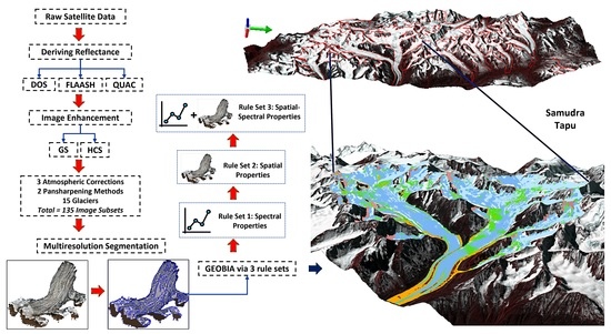
  • Rule Set 1: Only object spectral information
    This rule set utilizes only spectral information from the mean values per band and customized ratios developed from the mean values to classify objects, the reasoning being to test the level of accuracy achievable when classifying objects using only spectral properties.
  • Rule Set 2: Inter-object and contextual information
    This rule set utilizes features that are not direct object spectral properties or ratioed spectral properties. This rule set will test classification of segmented objects without direct information on the spectral properties of the object.
  • Rule Set 3: Combination of spectral and contextual information
    This rule set will attempt to combine the features of both rule sets to achieve the best possible classification map. Supplementary Table S3 presents the exact rule set post segmentation for all the processing schemes. Table 3 highlights the best performing rule sets for the associated processing scheme for both study areas based on individual overall accuracy and F1 score.
Figure 5 displays the classification results of the rule sets and processing schemes displayed in Table 3.

3.4. Accuracy Assessment

Logistical constraints in the field campaign to Svalbard, and harsh field conditions in the month of image acquisition in the Himalaya, prohibited ground truth collection. Avoiding bias in the manual assignment of reference data, a total of 1160 points were selected in an equalized random-sampling approach [42,43] to determine the accuracy of the thematic results. Error matrices were generated to calculate measures such as precision, recall, F1 score, overall accuracy (OA), error rate, and specificity [44]. While error rate is calculated as ‘100-OA’ in terms of percentage, Supplementary Table S4 highlights the mathematical equations of the measures.

4. Results and Discussion

4.1. Quantitative Analysis of Surface Facies

4.1.1. Area of Surface Facies for Each Processing Scheme

The area of each facies is reported as an average across the rule sets for each individual processing scheme. Table 4 highlights the area per facies for glaciers ST and ML.
Glaciers in Ny-Ålesund are smaller in size when compared to glaciers in the Chandra–Bhaga basin. Owing to this, the variances in area of facies are greater for ST classification than the ML classification. Figure 6 presents the deviations from the average classified area for all facies across glaciers ML and ST using stacked bar graphs. For the ST glacier, cumulative variances across all processing schemes highlight that the atmospherically corrected, non-sharpened imageries (average of DOS, FLAASH, and QUAC) deliver the highest variance of 2.78 km2. Among the individual subsets, FLAASH provides the least variance across all facies (0.76 km2). The maximum variation was delivered by the QUAC subsets. The GS sharpened subsets provide moderate variance with an average of 2.54 km2. The HCS subsets deliver the least variance in the classified area (13.68 km2) among the facies for the ST glacier. Within the facies themselves, glacier ice observes the most cumulative variations in classified area, whereas shadowed snow varies the least.
Unlike the ST classifications, the ML facies show an inverse trend of variability according to pansharpening. The pansharpened subsets report slightly higher cumulative average variances for the GS and HCS subsets (0.10 and 0.11 km2) than the non-pansharpened subsets (0.09 km2). Within the individual subsets the QUAC delivers least variability. Among the facies, dry snow retains maximum consistency across all processing schemes with a variance in classified area of 0.02 km2. Glacier ice shows maximum variation at 0.19 km2.

4.1.2. Accuracy Yielded by Each Rule Set

Complete accuracy assessment for the classification is detailed in Supplementary Sheet S1. Here, we aim to assess the classification results of the rule sets using the F1 score [44] as an average of all processing schemes/subsets. The aim is to utilize the robustness of the F1 score to determine reliability of the classified surface facies and rule sets. This is followed by the OA to delineate the order of reliable classification across both study areas and as an average of both study areas. Figure 7 highlights the F1 score of the classified facies averaged across all processing schemes for each rule set along with the respective deviation from the mean.
Overall observations suggest that rule set 3 delivered the best performance for both study sites. In the case of Ny-Ålesund classifications, it is observed that rule set 1 provides the least variance in mapped facies. However, the inability of spectral information to isolate fine features such as streams and crevasses is a major limiting factor. Rule set 2, which primarily utilizes spatial and contextual information, is limited by the large variations in performance across all processing schemes. An inference is possible here that different preprocessing routines may influence the spatial and contextual characteristics of objects to a greater extent than absolute spectral information. Unfortunately, this finding does not extend to facies in the Chandra–Bhaga basin. Here, rule set 2 delivered the median variance between rule set 1 and 3. The variance for the Chandra–Bhaga rule set 2 classification is less (0.06) than the Ny-Ålesund rule set 2 classifications (0.16). The better performance of the Chandra–Bhaga classifications suggests that fewer classes with better spectral separability can result in better thematic classifications across all processing schemes by combining spatial–spectral attributes. Hence, the implication from these results highlights the decrease in impact of processing schemes on VHR imagery for facies with larger spectral separability and a lower number of classes and by utilizing spatial–spectral attributes. Table 5 summarizes the OA and the reliability orders for mapped facies and the study sites. The reliability orders highlight the best combination of features (Table 3 and Supplementary Table S3) that enabled mapping of the facies with the highest calculated accuracy.

4.1.3. Variable Effect of Atmospheric Corrections

Figure 8 highlights the error rate yielded by each rule set for the atmospherically corrected image subsets. Rule set 3 delivers the most consistent performance, i.e., the lowest error rate except for the Himalaya FLAASH_Rule Set 1 classification. The common highest error rate was observed for both the Ny-Ålesund QUAC_Rule Set 1 and Ny-Ålesund FLAASH_Rule Set 2 classifications. When based upon variances in the performance of processing schemes, the reliability order of atmospheric corrections is DOS > FLAASH > QUAC.
Rule set 3 delivers the most consistent performance, i.e., the lowest error rate except for the Himalaya FLAASH_Rule Set 1 classification. The common highest error rate was observed for both the Ny-Ålesund QUAC_Rule Set 1 and Ny-Ålesund FLAASH_Rule Set 2 classifications. When based upon variances in performance of processing schemes, the reliability order of atmospheric corrections is DOS > FLAASH > QUAC. The reliability of individual rule sets based upon the error rate is Ny-Ålesund QUAC_Rule Set 3 > Ny-Ålesund DOS_Rule Set 3 = Ny-Ålesund FLAASH_Rule Set 3 > Ny-Ålesund DOS_Rule Set 2 > Ny-Ålesund QUAC_Rule Set 2 > Himalaya DOS_Rule Set 3 > Himalaya FLAASH_Rule Set 1 > Himalaya DOS_Rule Set 2 = Himalaya QUAC_Rule Set 2 = Himalaya QUAC_Rule Set 3 > Himalaya QUAC_Rule Set 1 > Ny-Ålesund FLAASH_Rule Set 1 > Himalaya FLAASH_Rule Set 3 > Ny-Ålesund DOS_Rule Set 1 = Himalaya DOS_Rule Set 1 = Himalaya FLAASH_Rule Set 2 > Ny-Ålesund QUAC_Rule Set 1 = Ny-Ålesund FLAASH_Rule Set 2.
These findings imply that when combining spatial–spectral properties of objects, the DOS correction is sufficient for deriving reliable and accurate thematic classifications. FLAASH is most useful when the mapping procedure relies purely on spectral information. QUAC and DOS deliver similar performances for rule set 2, and this suggests that GEOBIA relying heavily on spatial properties between objects would benefit from simpler corrections. In a comparative assessment using GEOBIA for mapping benthic habitats, Siregar et al. [45] suggested that the difference between FLAASH corrected and noncorrected classification is not significant. However, the profile used to highlight post correction spectral signatures highlights that the range of reflectance was not resampled from 0 to 1. Moreover, as the classification was performed using support vector machines (SVM) post segmentation, a comparison between rule-set-based classification is difficult. While the high performance of the DOS correction in the current study does not agree with the findings of Phiri et al. [46], it is likely because the current study utilizes rule sets rather than a classification algorithm (such as random forest) to classify segmented objects. Moreover, the superior performance of DOS is due to the combination of spatial and spectral properties, whereas FLAASH performs better for only spectral properties. This is important because where PBIA relies solely on spectral properties, GEOBIA can utilize spatial–spectral properties to overcome computational loads of complex atmospheric corrections.

4.1.4. Impact of Pansharpening

Table 6 depicts the average performance of pansharpened imagery across all three rule sets utilizing the OA as the assessing measure. Figure 9 highlights the OA for pansharpened, and non-sharpened images averaged across all the rule sets.
Considering rule set 1, neither GS nor HCS enhanced the OA for DOS and FLAASH subsets. HCS and GS added minor accuracy improvements to the QUAC subsets. Rule set 2 displayed the greatest loss in performance after pansharpening. The HCS_FLAASH reduced in performance by 15.84%. This is a significant decrease in OA. However, rule set 3 classifications showed enhancements in the OA of GS_FLAASH, HCS_DOS, and HCS_QUAC. Averaging across rule sets, the performance trend for the pansharpened subsets is GS_QUAC > GS_FLAASH > GS_DOS = HCS_QUAC > HCS_DOS > HCS_FLAASH. Overall comparison between pansharpening algorithms suggest that GS > HCS. Of all pansharpened image rule sets, rule set 3 delivered maximum performance and rule set 2 was the most inaccurate. This is surprising, as finer resolution can improve the contrast between image pixels, allowing for potentially better segregation of homogenous objects [47]. Rule set 2, which relies on the spatial distinction between objects, decreased in accuracy after pansharpening. Gavankar and Ghosh [48] utilized HCS sharpened Ikonos imagery to identify buildings in an urban setting. Buildings usually have consistent geometric shapes; this consistency can be leveraged using shape parameters such as circulometry and rectangulomtery [48]. A glacier’s surface does not contain consistent geometric patterns, and this may indicate that segmentation of fine-resolution satellite data does not necessarily translate to improved classification. In a post-earthquake GEOBIA-based mapping application to identify damaged buildings and temporary relief sites, Omarzdeh et al. [49] found that damaged buildings which have lost their consistent structure are difficult to map. This inconsistency due to shape can also be detrimental for glacier facies mapping, as developing rules to accurately depict textural variations in observed facies is a challenge. Rule set 2 is testament to the challenges of spatial property-based mapping. The importance of combined spatial–spectral characteristics is evident, as segmentation can compensate the pansharpened image with high frequency information inserted during pansharpening [50].

4.2. Discussion

In the quest of mapping earth features through GEOBIA, the focus is usually on multi-level/scale segmentation to highlight finer features. Glacier surfaces have a variety of undulating and disheveled features such as crevasses and debris which may necessitate such segmentation. However, in the current study, we focused on attempting to adapt the object features post segmentation to discern the visible surface facies. Utilizing only spectral information, streams and crevasses were not defined in any rule set 1 for Ny-Ålesund. In the case of Himalayan facies, crevasses were highlighted using all rule sets. This may be because the crevasses in Himalayan facies are larger and more clearly discernible than in Ny-Ålesund. Mitkari et al. [23] found some rills that were misclassified with periglacial debris in their multi-source GEOBIA approach on the Bara Shigri glacier. This is attributed to the coarser scale of segmentation. In the current study, however, the finer streams and crevasses were not classified using only spectral information. The contextual and spatial attributes of rule set 2 and rule set 3 enabled the identification of streams and crevasses. The standard deviation feature was most useful for discerning the minor streams and crevasses. This may point towards certain spatial attributes that can overcome the spectral constraints. Kim et al. [16] found that addition of the GLCM to multi-scale and single-scale segmentation improved classification performance. Moreover, the same constraint was found in the current study when mapping the same features using pansharpened images. Dabiri et al. [51] utilized Landsat images to perform landslide mapping using thresholds on indices and layer values in OBIA. However, due to acquisition of different images under different illumination conditions, each image was assigned thresholds independently. In the current study, differing processing routines cause a change in the derived reflectance [paper 1]. This therefore implies that the thresholds and object features utilized must be assigned accordingly. Each rule set for each processing scheme was assigned independently. It is observed that the maximum variation in rule sets is required in processing schemes for the Ny-Ålesund image, whereas most of the Himalayan images were classified with similar features, albeit with changes in the thresholds owing to changes in reflectance. This suggests that fewer features and larger targets can be extracted with more stable rule sets using changes in thresholds according to image and scene conditions. However, smaller features necessitate more rigorous processing. Rastner et al. [9] found that pixel-based mapping outperformed OBIA when detecting objects with single pixel size such as nunataks, narrow ridges, and couloirs. However, their analysis was performed on Landsat ETM+, ASTER, and Landsat TM imagery. In the case of the current study, the streams and crevasses in Ny-Ålesund were mapped using spatial attributes. A key finding is that improvement in spatial resolution did not necessitate a change in segmentation parameters. Furthermore, the same segmentation was applicable on all processing schemes, and this suggests that irrespective of the processing routines the combination of ‘optimal’ segmentation when combined with adjusted spatial and spectral attributes is sufficient for mapping glacier surface facies using VHR data.
In paper 1, we analyzed the variations induced by different processing routines in the thematic classification of facies using conventional and advanced pixel-based classification methods. In this study, we analyzed the impact of the same processing routines on GEOBIA mapping of surface facies. In paper 1, the FLAASH algorithm performed the best, whereas here, the DOS-based rule sets delivered superior performance. Pansharpening significantly reduced reliability of PBIA, whereas it selectively improved overall performance in OBIA. This highlights that segmentation and spatial–spectral attributes have a key advantage over hard pixel classification using VHR VNIR satellite data.

Significances and Challenges

GEOBIA classifications can be categorized into (a) operator driven (rule sets) and (b) operator assisted (classification algorithms). Johnson et al. [52] labels these groups as knowledge driven and automated classification. In the current study, we focus on rule sets because although semi-automated approaches are reported to be less subjective [52], rigorous analysis of individual object characteristics to identify meaningful segmentation and useful spatial–spectral features must be performed to gauge the quality of classification. Rule sets can be described as an attempt to replicate logical patterns of image interpretation from the human brain into classification operations [47]. The impact of processing routines on the modification of rule sets presents an opportunity to identify necessary changes in feature thresholds. The data of variation in thresholds, applicability of indices, and spectral information for each processing routine can also help drive the direction of semi-automated classification. Deep learning approaches such as SVM [45] and random forest (RF) [46] can be applied after OBIA to turn the classification into a semi-automatic process. However, the selection of the preprocessing method, the collection of training data, and the resultant goal of mapping facies using any GEOBIA method require a foundational test of the impact of these methods. Rule sets offer the best capacity for object-by-object analysis for many GEOBIA mapping applications and can be compared with results of semi-automatic methods. In this study, each rule set was defined by carefully testing all the parameters associated with the respective facies under consideration and the object features that can enable clear delineation of the target. For Ny-Ålesund, rule set 1 was not capable of differentiating streams and crevasses. This class was misclassified between dirty ice and saturated snow across all processing schemes. Enhancing spatial resolution did not improve mapping of fine features, although the overall classification did improve in cumulative accuracy. The variations in rule sets across processing schemes are found to be greater when the number of surface facies are greater, and the classes have a greater probability of spectral overlap. In such scenarios, scene-based adjustments are necessary for more accurate mapping [53]. However, as demonstrated in this study, spatial attributes may help overcome spectral complexities.
Shadowed areas in the Himalayan images were classified using an overlap of manually digitized vector data. This was constant throughout the experiment. However, the same issue did not arise in the classification of shadowed snow in Ny-Ålesund. Unfortunately, no index or mean threshold parameter was useful in delineating shadowed snow. This is a persistent problem in mountain glacier classification [54]. Figure 10 displays the spectral signatures of the shadowed areas on different points on the FLAASH subset of the glaciers. Figure 11 presents the variations in spectral reflectance of each of the processing schemes. In Figure 10, spectral pattern 2 shows a combination of saturated snow and dry/wet snow. Spectral patterns 3 and 4 are combinations of wet snow, melting snow, and saturated snow. Figure 10b highlights the variations in shadowed snow on the ST glacier. Figure 10b spectral pattern 2 does not even follow the same trend in reflectance. Patterns 1, 3, 4, and 5 vary in intensity, and these variations are significant when derived on other processing schemes (Figure 11). Using the atmospheric corrections in the current study, shadowed areas could not be divided into their constituent facies. Ryan et al. [55] and Leidman et al. [56] noted that shadowed areas can cause overestimation of darker classes. To avoid misclassification between streams and crevasses, dirty ice (the facies with the lowest reflectance), and the snow facies within the shadow, all shadowed areas were labelled as shadowed ‘snow’. Shadows induced by larger features present challenges in the classification of smaller features lying within the shadow area. In such cases, the presence of more spectral bands and operator innovation is necessary for creative application of object features [49]. The aim of the current study is to focus on the impact of basic image-processing routines on GEOBIA mapping of glacier facies. The time needed for manual assignment of rules is immense. In this case, corrections for shadows were beyond scope. Moreover, differentiating between glacier features under shadowed areas is more problematic for large-scale mapping applications. Breaking down the component facies of shadowed areas on many glaciers would be an engaging challenge for future experiments. Ancillary layers have been used to supplement GEOBIA [19,23]. This study does not utilize multi-source datasets and highlights the capabilities of a combination of object features to map surface facies.
The Himalayan image shows a larger distribution of snow for its acquisition period. Unfortunately, free precipitation data are not available to corroborate this snow cover with a sudden precipitation event. Currently, free precipitation data for this region are only available from 1901 to 2002 [57]. Estimation of snow cover areas (SCA) and the trend of SCA variability for this region may help support any increase in snow cover during the period of acquisition. Prior to this, it is important to distinguish between SCA and surface facies mapping. SCA mapping is more often performed at a basin level or larger regional scale encompassing a coarser resolution for analyzing spatial, hypsographic, and temporal variability [58]. For example, the Moderate Resolution Imaging Spectroradiometer (MODIS) global snow cover product MOD10CM outlines SCA at a spatial resolution of 5 km [59]. Glacier surface facies are all the zones of snow and ice which can be distinguished based on visual and spectral properties. These facies are clearly visible at the end of the summer season, when almost all the seasonal snow has disappeared. While SCA operations can consider an entire glacier to be ‘snow’, facies mapping operations may divide snow into dry, wet, melting, saturated, etc. At the basin level and larger, SCA is reported to have substantially reduced [60]. However, at the sub-basin level, snow cover is reported to have greater dynamicity [61]. Rathore et al. [61] analyzed SCA variability and accumulation and ablation patterns using daily snow cover data from 2004 to 2014 for six sub-basins of the Chenab basin, which include the Chandra and Bhaga basins of the current study. The imagery used in the present study covers part of the Chandra and part of the Bhaga sub-basins. Hence, the name used here is the Chandra–Bhaga (sub)basin of the current study. Rathore et al. [61] observed an increasing trend in maximum snow cover during the accumulation period. Sub-basins such as Ravi and Warwan showed greater variability in the snow cover due to simultaneous accumulation and ablation, whereas the Chandra–Bhaga area did not display such variability. The larger distribution in snow cover in Chandra–Bhaga was attributed to the higher elevation of the sub-basin in comparison to the others. The authors even observed full coverage of snow even at temperatures of 13 °C. This is suggested to be because of melt causing a reduction in thickness, but not area. Moreover, precipitation data collected using an all-weather station (AWS) in the Bhaga basin suggests that rainfall (wet precipitation) is decreasing, whereas snowfall (dry precipitation) is not. SCA for the month of October also highlights a greater distribution of snow for the year 2014 than 2010–2013 [61]. Sahu and Gupta [62] report similar findings for seasonal analysis of SCA in the Chandra basin from 2000–2017. The authors observed that SCA begins increasing from September due to lower temperatures. This effectively corroborates the large distribution of snow observed and classified in the Chandra–Bhaga basin in the present study.
Unlike the Chandra–Bhaga basin, glaciers in Svalbard are experiencing accelerated thinning [63,64]. The ML glacier in Ny-Ålesund contains the longest record of observed data [65]. The Equilibrium Line Altitude (ELA) determines the transition from accumulation facies to ablation facies. Average elevation of the maximum snowline in summer can be used as a representative ELA [65]. The various snow facies in the ML glacier identified here comprise dry snow, wet snow, melting snow, saturated snow, and shadowed snow. The facies are based on visual assessments and spectral characteristics with comparisons against the literature [paper 1]. The image was acquired at the end of the ablation season in August 2016, and this implies that most of the seasonal snow has disappeared, leaving the full range of facies. As precipitation largely determines the ELA, it would be lower in Ny-Ålesund, as the region is closer to the coast [65,66]. The ELA estimated by Pelt et al. [65] is available until 2012. Recently, Garg et al. [67] mapped radar facies at the same site. They utilized the boundary of percolation/wet snow and clean ice as the ELA. Their analysis was performed on seasonal data for the years 2016 to 2020. The year 2016 was marked by an increase in winter season temperature and spring temperature. This invariably would cause an increase in the melt of accumulated snow, thus increasing the amount of wet snow adjacent to dry/perennial snow. This dry snow facies was not discernible in the observation made by Garg et al. [67]. However, in the current study, dry snow was characterizable using VHR multispectral characteristics and GEOBIA. The ELA is reported to be shifting upward due to increasing temperature and reduced precipitation [67]. Precipitation data for Ny-Ålesund for the month and year of image acquisition [68] show no sudden precipitation event prior to scene capture. This suggests that the facies maps and the rule sets are not impacted by any sudden increase in snow.
Increasing temperature in glaciated areas also raises the necessity for identifying and mapping permafrost. According to the National Snow and Ice Data Center (NSIDC), permafrost is a layer of soil/rock, at some depth below the surface, where the temperature has been continuously below 0 °C for a few years or where summer heat does not penetrate to the basal layer of frozen ground [69]. Dabski [70] describes the presence of permafrost in the periglacial and foreland area of a polythermal glacier. The author further highlights the difficulty in discerning between glacial and periglacial domains in high mountain and polar areas [71]. The primary mechanisms for identifying and measuring permafrost are through physical assessments in boreholes, geophysical sounding, temperature logging, and modelling [72]. As it is a subsurface phenomenon, permafrost can itself be difficult to observe using RS data [60]. The observable surface phenomenon is the active layer (lying above permafrost), which freezes, thaws, and refreezes seasonally. This layer can be measured either directly or by interpolation of 0 °C isotherm derived from borehole measurements [73,74]. Using data of mean annual ground temperature, depth of zero annual amplitude, and active layer thickness from the Global Terrestrial Network for Permafrost (GTN-P) database [75,76], Karjalainen et al. [77] predicted the risks of permafrost thaw. Much of the data within the GTN-P database comes from the Thermal State of Permafrost (TSP) Snapshot Borehole Inventory [78,79]. Westermann et al. [80] described two methods for characterizing permafrost using remote observations: (a) mapping landforms indicative of the presence of permafrost, and (b) characterizing and isolating physical variables that correspond to thermal subsurface phenomena. This requires penetrative radar to account for the freeze–thaw state and modelling of land surface temperature (LST) [81]. In the current experiment, we only rely on VNIR VHR multispectral data and thus can neither model LST nor identify subsurface conditions. Incorporating complex permafrost modelling into GEOBIA would be a challenge beyond the scope of the current study. Currently, global permafrost zonation maps are available at a spatial resolution of 1 km [81]. In this study, digitized glacial boundaries were used to extract the glaciers from the study sites, and a 3D visualization of ice divides was used to ensure maximum efficiency. Due to this, it was not necessary to isolate the glacial and periglacial margins. However, the process of permafrost extraction using a combination of RS datasets can be a promising, albeit challenging, direction.
We acknowledge the lack of field data for validation. However, the main aim of the experiment was to test the impact that various processing routines have on the final classification of glacier surface facies. The comparison between the SCA derived in the current study against previous findings along with the equalized random sampling approach and rigorous analysis of performances aid the robustness of the current study. As travel restrictions due to the COVID-19 pandemic did not permit a field campaign during the experiment, visual and spectral characteristics of facies were compared against the literature for their validity [21] (paper 1). A major limitation is the time needed to manually adjust rule sets for each processing scheme. Nevertheless, this works to our advantage in analyzing the implementation of GEOBIA for specific processing schemes. To the best of our knowledge, no study has yet tested the impacts of various processing schemes and rule sets on the thematic classification of glacier surface facies using GEOBIA. An important part of GEOBIA is the transferability of methods. Through the current study, we infer that even for the same sensor over the same glacier, the influence of processing routines dictates the thresholds of spectral features. However, the segmentation parameters tested here may be transferable, as they have consistently yielded optimal objects.

5. Conclusions

This study aimed to map glacier surface facies using a multi-rule set GEOBIA approach utilizing varying image-processing schemes to test the robustness of segmentation and reliability of rule sets. Three atmospheric corrections and two pansharpening algorithms were tested on VHR VNIR WV-2 for Ny-Ålesund and Chandra–Bhaga basin, Himalaya. The atmospheric correction methods included DOS, QUAC, and FLAASH. The pansharpening methods included GS and HCS. The selected segmentation parameters delivered consistent results across all processing schemes. A series of object features were identified to create three rule sets. Rule set 1 focused on only spectral information and rule set 2 relied on contextual and inter-object features, whereas rule set 3 combined both spatial and spectral information. Among the atmospheric corrections, DOS delivered the highest overall accuracy, followed by QUAC, and lastly FLAASH. Pansharpening improved overall performance with GS delivering greater accuracy than HCS. For the Ny-Ålesund glaciers, dirty ice, glacier ice, saturated snow, melting snow, wet snow, and streams and crevasses were best mapped by rule set 3, whereas dry snow and melting glacier ice were best mapped by rule set 1. For the Chandra–Bhaga basin glaciers, all facies were best mapped by rule set 3.
The current study highlights the requirement of selection of segmentation parameters. The incorporation of thresholds differed across rule sets, indicating a more processing-focused, in-scene, and image-specific approach for mapping applications of surface facies. Nevertheless, the segmentation parameters may be transferable to other VHR VNIR data. GEOBIA offers the capability of combining spatial–spectral attributes to glacier surface facies mapping, which can transcend the distortions in performance induced in PBIA by variable processing routines. Moreover, the classification is performed entirely devoid of ancillary data such as slope and temperature, enabling a much deeper understanding of the potential of VHR VNIR data for mapping glacier surface facies.

Supplementary Materials

The following supporting information can be downloaded at: https://0-www-mdpi-com.brum.beds.ac.uk/article/10.3390/rs14174403/s1, Table S1: The selected glaciers of the study, their areal extents, and GLIMS reference IDs. The extents were calculated from the delineated shapefiles using the geometry calculator in ArcGIS; Table S2: Spectral-band-wise at-sensor reflectance values of selected dark pixels for input into DOS correction module in ENVI 5.3. Table S3: Stepwise rule sets and threshold delineation for each processing scheme for both study sites. The ratios used here are highlighted in Table 2. Table S4: Measures of accuracy used in the current study. TP: samples are those that are in the positive class and are correctly classified, TN: samples that are correctly classified as negative, FP: samples that are not truly of the positive class but are incorrectly mapped as positive. FN: samples that are mapped as negative when they are positive. Sheet S1: Precision, recall, specificity, F1 score. Overall accuracy (OA), error rate (ER) for each processing scheme, rule sets, facies, and both study sites.

Author Contributions

Conceptualization and experiment setup, S.D.J. and S.F.W.; methodology and manuscript design, S.D.J. and S.F.W.; software and processing, S.D.J. and S.F.W.; validation, S.D.J. and S.F.W.; result analysis and discussion, S.D.J. and S.F.W.; resources, A.J.L. and K.B.; writing—original draft preparation, S.F.W. and S.D.J.; writing—review and editing, S.D.J., A.J.L. and K.B.; visualization, S.F.W.; supervision, S.D.J., A.J.L. and K.B.; project administration, S.D.J., A.J.L. and K.B. All authors have read and agreed to the published version of the manuscript.

Funding

This research received no external funding.

Data Availability Statement

Freely available data used in the current study—(1) ASTER GDEM v2. Downloaded from: Gdex.cr.usgs.gov/gdex/ (accessed on: 2 February 2017). The data are now moved to GDEM v3: (reviewed on: 12 March 2022) ASTER GDEM is a product of Japan’s Ministry of Economy, Trade, and Industry (METI) and NASA. (2) Arctic DEM. Available online: Pgc.umn.edu/data/arcticdem/ (accessed on: 21 January 2019).

Acknowledgments

The authors would like to thank DigitalGlobe (now Maxar Technologies) for providing high-resolution satellite data. Chandra–Bhaga basin imagery WorldView-2 © 2014 Maxar Technologies; Ny-Ålesund imagery WorldView-3 © 2016 Maxar Technologies. The authors thank the reviewers for their constructive criticism, which helped improve the manuscript. The authors also thank HOD, Civil Engineering, and Director, MIT, MAHE for their support.

Conflicts of Interest

The authors declare no conflict of interest.

References

  1. Huss, M. Present and future contribution of glacier storage change to runoff from macroscale drainage basins in Europe. Water Resour. Res. 2011, 47, W07511. [Google Scholar] [CrossRef]
  2. Kulkarni, A.V.; Randhawa, S.S.; Rathore, B.P.; Bahuguna, I.M.; Sood, R.K. Snow and glacier melt runoff model to estimate hydropower potential. J. Indian Soc. Remote Sens. 2002, 30, 221–228. [Google Scholar] [CrossRef]
  3. Gaddam, V.K.; Boddapati, R.; Kumar, T.; Kulkarni, A.V.; Bjornsson, H. Application of “OTSU”—An image segmentation method for differentiation of snow and ice regions of glaciers and assessment of mass budget in Chandra basin, Western Himalaya using Remote Sensing and GIS techniques. Environ. Monit. Assess. 2022, 194, 337. [Google Scholar] [CrossRef] [PubMed]
  4. Bolch, T.; Menounos, B.; Wheate, R. Landsat-based inventory of glaciers in western Canada, 1985–2005. Remote Sens. Environ. 2010, 114, 127–137. [Google Scholar] [CrossRef]
  5. Gore, A.; Mani, S.; HariRam, R.P.; Shekhar, C.; Ganju, A. Glacier surface characteristics derivation and monitoring using Hyperspectral datasets: A case study of Gepang Gath glacier, Western Himalaya. Geocarto Int. 2017, 34, 23–42. [Google Scholar] [CrossRef]
  6. Braun, M.; Schuler, T.V.; Hock, R.; Brown, I.; Jackson, M. Comparison of remote sensing derived glacier facies maps with distributed mass balance modelling at Engabreen, northern Norway. IAHS Publ. Ser. Proc. Rep. 2007, 318, 126–134. [Google Scholar]
  7. Avanzi, F.; Gabellani, S.; Delogu, F.; Silvestro, F.; Cremonese, E.; di Cella, U.M.; Ratto, S.; Stevenin, H. Snow Multidata Mapping and Modeling (S3M) 5.1: A distributed cryospheric model with dry and wet snow, data assimilation, glacier mass balance, and debris-driven melt. Geosci. Model Dev. 2022, 15, 4853–4879. [Google Scholar] [CrossRef]
  8. Jawak, S.D.; Wankhede, S.F.; Luis, A.J.; Balakrishna, K. Impact of Image-Processing Routines on Mapping Glacier Surface Facies from Svalbard and the Himalayas Using Pixel-Based Methods. Remote Sens. 2022, 14, 1414. [Google Scholar] [CrossRef]
  9. Rastner, P.; Bolch, T.; Notarnicola, C.; Paul, F. A Comparison of Pixel-and Object-Based Glacier Classification with Optical Satellite Images. IEEE J. Sel. Top. Appl. Earth Obs. Remote Sens. 2014, 7, 853–862. [Google Scholar] [CrossRef]
  10. Guo, S.; Du, P.; Xia, J.; Tang, P.; Wang, X.; Meng, Y.; Wang, H. Spatiotemporal changes of glacier and seasonal snow fluctuations over the Namcha Barwa–Gyala Peri massif using object-based classification from Landsat time series. ISPRS J. Photogramm. Remote Sens. 2021, 177, 21–37. [Google Scholar] [CrossRef]
  11. Hay, G.J.; Castilla, G. Geographic Object-Based Image Analysis (GEOBIA): A New Name for a New Discipline. In Object-Based Image Analysis; Springer: Berlin/Heidelberg, Germany, 2021; pp. 75–89. [Google Scholar]
  12. Blaschke, T. Object based image analysis for remote sensing. ISPRS J. Photogramm. Remote Sens. 2010, 65, 2–16. [Google Scholar] [CrossRef] [Green Version]
  13. Lang, S. Object-Based Image Analysis for Remote Sensing Applications: Modeling Reality–Dealing with Complexity. In Object-Based Image Analysis; Springer: Berlin/Heidelberg, Germany, 2008; pp. 3–27. [Google Scholar]
  14. D’Oleire-Oltmanns, S.; Marzolff, I.; Tiede, D.; Blaschke, T. Detection of Gully-Affected Areas by Applying Object-Based Image Analysis (OBIA) in the Region of Taroudannt, Morocco. Remote Sens. 2014, 6, 8287–8309. [Google Scholar] [CrossRef]
  15. Willhauck, G.; Schneider, T.; De Kok, R.; Ammer, U. Comparison of object-oriented classification techniques and standard image analysis for the use of change detection between SPOT multispectral satellite images and aerial photos. Int. Arch. Photogramm. Remote Sens. 2000, 33 Pt B3, 35–42. [Google Scholar]
  16. Kim, M.; Warner, T.A.; Madden, M.; Atkinson, D.S. Multi-scale GEOBIA with very high spatial resolution digital aerial imagery: Scale, texture and image objects. Int. J. Remote Sens. 2011, 32, 2825–2850. [Google Scholar] [CrossRef]
  17. Verhagen, P.; Drăguţ, L. Object-based landform delineation and classification from DEMs for archaeological predictive mapping. J. Archaeol. Sci. 2012, 39, 698–703. [Google Scholar] [CrossRef]
  18. Höfle, B.; Geist, T.; Rutzinger, M.; Pfeifer, N. Glacier surface segmentation using airborne laser scanning point cloud and intensity data. Int. Arch. Photogramm. Remote Sens. Spat. Inf. Sci. 2007, 36 Pt 3, W52. [Google Scholar]
  19. Robson, B.; Nuth, C.; Dahl, S.; Hölbling, D.; Strozzi, T.; Nielsen, P. Automated classification of debris-covered glaciers combining optical, SAR and topographic data in an object-based environment. Remote Sens. Environ. 2015, 170, 372–387. [Google Scholar] [CrossRef]
  20. Sharda, S.; Srivastava, M. Classification of Siachen Glacier Using Object-Based Image Analysis. In Proceedings of the 2018 International Conference on Intelligent Circuits and Systems (ICICS), Phagwara, India, 19–20 April 2018. [Google Scholar]
  21. Jawak, S.D.; Wankhede, S.F.; Luis, A.J. Explorative Study on Mapping Surface Facies of Selected Glaciers from Chandra Basin, Himalaya Using WorldView-2 Data. Remote Sens. 2019, 11, 1207. [Google Scholar] [CrossRef]
  22. Farhan, S.B.; Kainat, M.; Shahzad, A.; Aziz, A.; Kazmi, S.J.H.; Shaikh, S.; Zhang, Y.; Gao, H.; Javed, M.N.; Zamir, U.B. Discrimination of Seasonal Snow Cover in Astore Basin, Western Himalaya using Fuzzy Membership Function of Object-Based Classification. Int. J. Econ. Environ. Geol. 2019, 9, 20–25. [Google Scholar]
  23. Mitkari, K.V.; Arora, M.K.; Tiwari, R.K.; Sofat, S.; Gusain, H.S.; Tiwari, S.P. Large-Scale Debris Cover Glacier Mapping Using Multisource Object-Based Image Analysis Approach. Remote Sens. 2022, 14, 3202. [Google Scholar] [CrossRef]
  24. Isaksen, K.; Nordli, Ø.; Førland, E.J.; Lupikasza, E.; Eastwood, S.; Niedźwiedź, T. Recent warming on Spitsbergen—Influence of atmospheric circulation and sea ice cover. J. Geophys. Res. Atmos. 2016, 121, 11913. [Google Scholar] [CrossRef]
  25. Raup, B.; Racoviteanu, A.; Khalsa, S.J.; Helm, C.; Armstrong, R.; Arnaud, Y. The GLIMS geospatial glacier database: A new tool for studying glacier change. Glob. Planet. Change 2007, 56, 101–110. [Google Scholar] [CrossRef]
  26. Digital Globe Product Details. Available online: https://www.geosoluciones.cl/documentos/worldview/DigitalGlobe-Core-Imagery-Products-Guide.pdf (accessed on 20 February 2020).
  27. ASTER GDEM v2. Available online: https://asterweb.jpl.nasa.gov/gdem.asp (accessed on 7 July 2022).
  28. Arctic DEM. Available online: Pgc.umn.edu/data/arcticdem/ (accessed on 21 January 2019).
  29. Porter, C.; Morin, P.; Howat, I.; Noh, M.-J.; Bates, B.; Peterman, K.; Keesey, S.; Schlenk, M.; Gardiner, J.; Tomko, K.; et al. “ArcticDEM”, Harvard Dataverse, V1. 2018. Available online: https://www.pgc.umn.edu/data/arcticdem/ (accessed on 13 March 2022).
  30. Atmospheric Correction User Guide. Available online: https://www.l3harrisgeospatial.com/portals/0/pdfs/envi/Flaash_Module.pdf (accessed on 20 November 2021).
  31. Kaufman, Y.; Wald, A.; Remer, L.; Gao, B.-C.; Li, R.-R.; Flynn, L. The MODIS 2.1-μm channel-correlation with visible reflectance for use in remote sensing of aerosol. IEEE Trans. Geosci. Remote Sens. 1997, 35, 1286–1298. [Google Scholar] [CrossRef]
  32. Abreu, L.W.; Anderson, G.P. The MODTRAN 2/3 report and LOWTRAN 7 model. Contract 1996, 19628, 132. [Google Scholar]
  33. Teillet, P.; Fedosejevs, G. On the Dark Target Approach to Atmospheric Correction of Remotely Sensed Data. Can. J. Remote Sens. 1995, 21, 374–387. [Google Scholar] [CrossRef]
  34. Zhang, Z.; He, G.; Zhang, X.; Long, T.; Wang, G.; Wang, M. A coupled atmospheric and topographic correction algorithm for remotely sensed satellite imagery over mountainous terrain. GIScience Remote Sens. 2017, 55, 400–416. [Google Scholar] [CrossRef]
  35. Rumora, L.; Miler, M.; Medak, D. Impact of Various Atmospheric Corrections on Sentinel-2 Land Cover Classification Accuracy Using Machine Learning Classifiers. ISPRS Int. J. Geo-Inform. 2020, 9, 277. [Google Scholar] [CrossRef]
  36. Bernstein, L.S.; Jin, X.; Gregor, B.; Adler-Golden, S.M. Quick atmospheric correction code: Algorithm description and recent upgrades. Opt. Eng. 2012, 51, 111719. [Google Scholar] [CrossRef]
  37. Pushparaj, J.; Hegde, A.V. Evaluation of pan-sharpening methods for spatial and spectral quality. Appl. Geomat. 2016, 9, 1–12. [Google Scholar] [CrossRef]
  38. Laben, C.A.; Brower, B.V. Process for Enhancing the Spatial Resolution of Multispectral Imagery Using Pan-Sharpening. U.S. Patent 6,011,875, 4 January 2000. [Google Scholar]
  39. Bhardwaj, A.; Joshi, P.; Snehmani; Sam, L.; Singh, M.; Singh, S.; Kumar, R. Applicability of Landsat 8 data for characterizing glacier facies and supraglacial debris. Int. J. Appl. Earth Obs. Geoinf. 2015, 38, 51–64. [Google Scholar] [CrossRef]
  40. Baatz, M.; Schape, A. Multiresolution Segmentation: An Optimization Approach for High Quality Multi-Scale Image Segmentation. In Angewandte Geographische Informations-Verarbeitung, XII; Strobl, J., Blaschke, T., Griesbner, G., Eds.; Wichmann Verlag: Heidelberg/Karlsruhe, Germany, 2000; pp. 12–23. [Google Scholar]
  41. Han, Y.; Javed, A.; Jung, S.; Liu, S. Object-Based Change Detection of Very High Resolution Images by Fusing Pixel-Based Change Detection Results Using Weighted Dempster–Shafer Theory. Remote Sens. 2020, 12, 983. [Google Scholar] [CrossRef]
  42. Keshri, A.K.; Shukla, A.; Gupta, R.P. ASTER ratio indices for supraglacial terrain mapping. Int. J. Remote Sens. 2009, 30, 519–524. [Google Scholar] [CrossRef]
  43. Richards, J.A. Remote Sensing Digital Image Analysis; Springer: Berlin/Heidelberg, Germany, 2013. [Google Scholar]
  44. Maxwell, A.E.; Warner, T.A. Thematic Classification Accuracy Assessment with Inherently Uncertain Boundaries: An Argument for Center-Weighted Accuracy Assessment Metrics. Remote Sens. 2020, 12, 1905. [Google Scholar] [CrossRef]
  45. Siregar, V.P.; Prabowo, N.W.; Agus, S.B.; Subarno, T. The effect of atmospheric correction on object based image classification using SPOT-7 imagery: A case study in the Harapan and Kelapa Islands. IOP Conf. Ser. Earth Environ. Sci. 2018, 176, 012028. [Google Scholar] [CrossRef]
  46. Phiri, D.; Morgenroth, J.; Xu, C.; Hermosilla, T. Effects of pre-processing methods on Landsat OLI-8 land cover classification using OBIA and random forests classifier. Int. J. Appl. Earth Obs. Geoinf. 2018, 73, 170–178. [Google Scholar] [CrossRef]
  47. Roganda, M.S.; Murti, S.H.; Widyatmanti, W. Mapping the distribution of natural ecosystems on peatlands through vegetation using the object-based image analysis (OBIA) method in Bangko district, Rokan Hilir regency, Riau. IOP Conf. Ser. Earth Environ. Sci. 2022, 1047, 012017. [Google Scholar] [CrossRef]
  48. Gavankar, N.L.; Ghosh, S.K. Object based building footprint detection from high resolution multispectral satellite image using K-means clustering algorithm and shape parameters. Geocarto Int. 2019, 34, 626–643. [Google Scholar] [CrossRef]
  49. Omarzadeh, D.; Karimzadeh, S.; Matsuoka, M.; Feizizadeh, B. Earthquake Aftermath from Very High-Resolution WorldView-2 Image and Semi-Automated Object-Based Image Analysis (Case Study: Kermanshah, Sarpol-e Zahab, Iran). Remote Sens. 2021, 13, 4272. [Google Scholar] [CrossRef]
  50. Witharana, C.; Civco, D.L.; Meyer, T.H. Evaluation of pansharpening algorithms in support of earth observation based rapid-mapping workflows. Appl. Geogr. 2013, 37, 63–87. [Google Scholar] [CrossRef]
  51. Dabiri, Z.; Hölbling, D.; Abad, L.; Prasicek, G.; Argentin, A.L.; Tsai, T.T. An Object-Based Approach for Monitoring the Evolution of Landslide-dammed Lakes and Detecting Triggering Landslides in Taiwan. Int. Arch. Photogramm. Remote Sens. Spat. Inf. Sci. 2019, 42, 103–108. [Google Scholar] [CrossRef]
  52. Johnson, B.A.; Tateishi, R.; Hoan, N.T. A hybrid pansharpening approach and multiscale object-based image analysis for mapping diseased pine and oak trees. Int. J. Remote Sens. 2013, 34, 6969–6982. [Google Scholar] [CrossRef]
  53. Shukla, A.; Ali, I. A hierarchical knowledge-based classification for glacier terrain mapping: A case study from Kolahoi Glacier, Kashmir Himalaya. Ann. Glaciol. 2016, 57, 1–10. [Google Scholar] [CrossRef]
  54. Lu, Y.; Zhang, Z.; Shangguan, D.; Yang, J. Novel Machine Learning Method Integrating Ensemble Learning and Deep Learning for Mapping Debris-Covered Glaciers. Remote Sens. 2021, 13, 2595. [Google Scholar] [CrossRef]
  55. Ryan, J.C.; Hubbard, A.; Stibal, M.; Irvine-Fynn, T.D.; Cook, J.; Smith, L.C.; Cameron, K.; Box, J. Dark zone of the Greenland Ice Sheet controlled by distributed biologically-active impurities. Nat. Commun. 2018, 9, 1065. [Google Scholar] [CrossRef]
  56. Leidman, S.; Rennermalm, Å.K.; Lathrop, R.G.; Cooper, M. Terrain-Based Shadow Correction Method for Assessing Supraglacial Features on the Greenland Ice Sheet. Front. Remote Sens. 2021, 2, 690474. [Google Scholar] [CrossRef]
  57. Free Precipitation Data for India. Available online: https://www.indiawaterportal.org/met_data (accessed on 14 August 2022).
  58. Desinayak, N.; Prasad, A.K.; El-Askary, H.; Kafatos, M.; Asrar, G.R. Snow cover variability and trend over the Hindu Kush Himalayan region using MODIS and SRTM data. Ann. Geophys. 2022, 40, 67–82. [Google Scholar] [CrossRef]
  59. Hall, D.K.; Riggs. MODIS/Terra Snow Cover Monthly L3 Global 0.05Deg CMG, Version 61; NASA National Snow and Ice Data Center Distributed Active Archive Center: Boulder, CO, USA, 2021. [Google Scholar] [CrossRef]
  60. Poloczanska, E. The IPCC Special Report on Ocean and Cryosphere in a Changing Climate-a view from the mountain tops to the deepest depths. In Proceedings of the 2020 Ocean Sciences Meeting, San Diego, CA, USA, 16–21 February 2020. [Google Scholar] [CrossRef]
  61. Rathore, B.P.; Singh, S.K.; Jani, P.; Bahuguna, I.M.; Brahmbhatt, R.; Rajawat, A.S.; Randhawa, S.S.; Vyas, A. Monitoring of snow cover variability in Chenab Basin using IRS AWiFS sensor. J. Indian Soc. Remote Sens. 2018, 46, 1497–1506. [Google Scholar] [CrossRef]
  62. Sahu, R.; Gupta, R.D. Snow cover area analysis and its relation with climate variability in Chandra basin, Western Himalaya, during 2001–2017 using MODIS and ERA5 data. Environ. Monit. Assess. 2020, 192, 489. [Google Scholar] [CrossRef]
  63. Kohler, J.; James, T.D.; Murray, T.; Nuth, C.; Brandt, O.; Barrand, N.E.; Aas, H.F.; Luckman, A. Acceleration in thinning rate on western Svalbard glaciers. Geophys. Res. Lett. 2007, 34, L18502. [Google Scholar] [CrossRef]
  64. Wang, Z.; Lin, G.; Ai, S. How long will an Arctic mountain glacier survive? A case study of Austre Lovénbreen, Svalbard. Polar Res. 2019, 38, 3519. [Google Scholar] [CrossRef]
  65. Van Pelt, W.J.; Kohler, J.; Liston, G.E.; Hagen, J.O.; Luks, B.; Reijmer, C.H.; Pohjola, V.A. Multidecadal climate and seasonal snow conditions in Svalbard. J. Geophys. Res. Earth Surf. 2016, 121, 2100–2117. [Google Scholar] [CrossRef]
  66. Hagen, J.O.; Kohler, J.; Melvold, K.; Winther, J.G. Glaciers in Svalbard: Mass balance, runoff and freshwater flux. Polar Res. 2003, 22, 145–159. [Google Scholar] [CrossRef]
  67. Garg, V.; Thakur, P.K.; Rajak, D.R.; Aggarwal, S.P.; Kumar, P. Spatio-temporal changes in radar zones and ELA estimation of glaciers in Ny-Ålesund using Sentinel-1 SAR. Polar Sci. 2022, 31, 100786. [Google Scholar] [CrossRef]
  68. Free Precipitation Data for Ny-Ålesund. Available online: https://seklima.met.no/observations/ (accessed on 14 August 2022).
  69. Concept of Permafrost from National Snow and Ice Data Center. Available online: https://nsidc.org/learn/parts-cryosphere/frozen-ground-permafrost (accessed on 23 August 2022).
  70. Dąbski, M. Should Glaciers Be Considered Permafrost? Geosciences 2019, 9, 517. [Google Scholar] [CrossRef]
  71. Berthling, I.; Schomacker, A.; Benediktsson, Í.Ö. The Glacial and Periglacial Research Frontier: Where from Here? In Treatise on Geomorphology; Shroder, J.F., Ed.; Elsevier: San Diego, CA, USA, 2013; pp. 479–499. [Google Scholar]
  72. Haeberli, W.; Noetzli, J.; Arenson, L.; Delaloye, R.; Gärtner-Roer, I.; Gruber, S.; Isaksen, K.; Kneisel, C.; Krautblatter, M.; Phillips, M. Mountain permafrost: Development and challenges of a young research field. J. Glaciol. 2010, 56, 1043–1058. [Google Scholar] [CrossRef]
  73. Christiansen, H.H.; Gilbert, G.L.; Demidov, N.; Guglielmin, M.; Isaksen, K.; Osuch, M.; Boike, J. Permafrost temperatures and active layer thickness in Svalbard during 2017/2018 (PermaSval). In SESS Report 2019-The State of Environmental Science in Svalbard; Svalbard Integrated Arctic Earth Observing System: Longyearbyen, Norway, 2020. [Google Scholar]
  74. Burn, C.R. The active layer: Two contrasting definitions. Permafr. Periglac. Processes 1998, 9, 411–416. [Google Scholar] [CrossRef]
  75. Biskaborn, B.K.; Lanckman, J.P.; Lantuit, H.; Elger, K.; Streletskiy, D.A.; Cable, W.L.; Romanovsky, V.E. The new database of the Global Terrestrial Network for Permafrost (GTN-P). Earth Syst. Sci. Data 2015, 7, 245–259. [Google Scholar] [CrossRef]
  76. Global Terrestrial Network for Permafrost Database. Available online: http://gtnpdatabase.org/ (accessed on 23 August 2022).
  77. Karjalainen, O.; Aalto, J.; Luoto, M.; Westermann, S.; Romanovsky, V.E.; Nelson, F.E.; Etzelmüller, B.; Hjort, J. Circumpolar permafrost maps and geohazard indices for near-future infrastructure risk assessments. Sci. Data 2019, 6, 190037. [Google Scholar] [CrossRef]
  78. International Permafrost Association (IPA). IPY 2007–2009 Thermal State of Permafrost (TSP) Snapshot Borehole Inventory, Version 1; National Snow and Ice Data Center: Boulder, CO, USA, 2010. [Google Scholar]
  79. Romanovsky, V.E.; Smith, S.L.; Christiansen, H.H. Permafrost thermal state in the polar Northern Hemisphere during the international polar year 2007–2009: A synthesis. Permafr. Periglac. Processes 2010, 21, 106–116. [Google Scholar] [CrossRef]
  80. Westermann, S.; Duguay, C.R.; Grosse, G.; Kaab, A. Remote sensing of permafrost and frozen ground. In Remote Sensing of the Cryosphere; Wiley-Blackwell: Hoboken, NJ, USA, 2015; pp. 307–344. [Google Scholar] [CrossRef]
  81. Obu, J.; Westermann, S.; Bartsch, A.; Berdnikov, N.; Christiansen, H.H.; Dashtseren, A.; Delaloye, R.; Elberling, B.; Etzelmüller, B.; Kholodov, A.; et al. Northern Hemisphere permafrost map based on TTOP modelling for 2000–2016 at 1 km2 scale. Earth-Sci. Rev. 2019, 193, 299–316. [Google Scholar] [CrossRef]
Figure 1. Geospatial location of the study areas. The 3D elevated surfaces are pansharpened images draped on digital elevation models. The insets of ML (WorldView-3 © 2016 Maxar Technologies) and ST (WorldView-2 © 2014 Maxar Technologies) are highlighted using the digitized boundary. The top image showing the global position of Svalbard and Chandra–Bhaga basin was prepared using Natural Earth (free vector and raster map data @ naturalearthdata.com).
Remotesensing 14 04403 g001
Figure 2. Methodology of the proposed study. MS: multispectral image; FLAASH: Fast Line-of-Sight Atmospheric Analysis of Hypercubes; QUAC: Quick Atmospheric Correction; DOS: Dark Object Subtraction; GS: Gram–Schmidt; HCS: Hyperspherical Color Sharpening; GEOBIA: Geographic Object-Based Image Analysis. The blue arrows from GS and HCS highlight the individual image subsets post pansharpening.
Remotesensing 14 04403 g002
Figure 3. Segmentation and classification on the ML FLAASH subset. (a) Non-segmented Image; (b) Segmented Object Mean View: Hidden Outlines; (c) Classified Merged Objects: Visible Object Outlines; (d) Classified Merged Objects: Hidden Outlines. RGB: Coastal, Blue, Green.
Remotesensing 14 04403 g003
Figure 4. Segmentation and classification on the ML GS_FLAASH subset. (a) Non-segmented Image; (b) Segmented Object Mean View: Hidden Outlines; (c) Classified Merged Objects: Visible Object Outlines; (d) Classified Merged Objects: Hidden Outlines. RGB: Coastal, Blue, Green.
Remotesensing 14 04403 g004
Figure 5. Classification results of the best rule sets from both study sites. Ny-Ålesund classification: (a) FLAASH_Rule Set 1; (b) DOS_Rule Set 2; (c) QUAC_Rule Set 3. Chandra-Bhaga Basin classification: (d) HCS_FLAASH_Rule Set 1; (e) HCS_QUAC_Rule Set 2; (f) HCS_FLAASH_Rule Set 3.
Remotesensing 14 04403 g005
Figure 6. Variations in classified area of each facies for the representative glaciers ML and ST. Stacked columns highlight variances in the classified area between processing schemes for the same facies.
Remotesensing 14 04403 g006
Figure 7. F1 score of each facies for the three rule sets as the mean of all processing schemes. The error bars in blue highlight deviations from the mean F1 score indicating reliability of the rule sets for the respective facies.
Remotesensing 14 04403 g007
Figure 8. Error rates (in %) of the rule sets for the atmospheric corrections presented as a donut diagram. Inner circle: rule set 1, middle circle: rule set 2, and outer circle: rule set 3.
Remotesensing 14 04403 g008
Figure 9. Overall-accuracy-based assessment of the performance of pansharpened vs. non-sharpened classifications. The 3D surface summarizes the OA from all three rule sets for (a) DOS vs. GS_DOS vs. HCS_DOS, (b) QUAC vs. GS_ QUAC vs. HCS_ QUAC, and (c) FLAASH vs. GS_FLAASH vs. HCS_FLAASH.
Remotesensing 14 04403 g009
Figure 10. Complex spectral patterns of the shadowed snow at different points on the glacier. Base images are the FLAASH corrected images draped on the ArcticDEM for Ny-Ålesund and ASTER GDEM v2 for Chandra–Bhaga basin. Inset (a) 3D surface of glacier ML, (b) 3D surface of glacier ST.
Remotesensing 14 04403 g010
Figure 11. Spectral reflectance of shadowed snow derived across all processing schemes. The left graph shows the reflectance of shadowed snow in Svalbard, whereas the graph on the right shows the reflectance of shadowed snow in the Himalayas.
Remotesensing 14 04403 g011
Table 1. Nomenclature of processing schemes and classifications used in the current study.
Nomenclature/AbbreviationDescription/Definition
DOSDOS-corrected
FLAASHFLAASH-corrected
QUACQUAC-corrected
GS_DOSDOS followed by GS sharpening
GS_FLAASHFLAASH followed by GS sharpening
GS_QUACQUAC followed by GS sharpening
HCS_DOSDOS followed by HCS sharpening
HCS_FLAASHFLAASH followed by HCS sharpening
HCS_QUACQUAC followed by HCS sharpening
DOS_Rule Set 1/2/3DOS followed by classification by any of the three rule sets
FLAASH_ Rule Set 1/2/3FLAASH followed by classification by any of the three rule sets
QUAC_ Rule Set 1/2/3QUAC followed by classification by any of the three rule sets
GS_DOS_ Rule Set 1/2/3DOS followed by GS followed by classification by any of the three rule sets
GS_FLAASH_ Rule Set 1/2/3FLAASH followed by GS followed by classification by any of the three rule sets
GS_QUAC_ Rule Set 1/2/3QUAC followed by GS followed by classification by any of the three rule sets
HCS_DOS_ Rule Set 1/2/3DOS followed by HCS followed by classification by any of the three rule sets
HCS_FLAASH_ Rule Set 1/2/3FLAASH followed by HCS followed by classification by any of the three rule sets
HCS_QUAC_ Rule Set 1/2/3QUAC followed by HCS followed by classification by any of the three rule sets
Table 2. Set of object, class, and customized features used to classify facies in this study. Description of the features in addition to the specific features used in the current study. Quantile [0.5] refers to the 50th percentile or middle quartile of the object data per spectral band.
Type of FeatureFeature NameDescriptionFeatures Tested in This Study
Object Features: Layer ValuesMean Value per Layer/BandThe mean layer intensity value of an image object [42]Coastal, Blue, Green, Yellow, Red, Red Edge, NIR 1, NIR 2, Brightness, Max. Difference
Object Features: Layer ValuesQuantileThe feature value, where a specified percentage of image objects from the selected image object have a smaller feature value [42]Quantile [0.5] (Coastal), Quantile [0.5] (Coastal), Quantile [0.5] (Blue), Quantile [0.5] (Green), Quantile [0.5] (Yellow), Quantile [0.5] (Red), Quantile [0.5] (Red Edge), Quantile [0.5] (NIR 1), Quantile [0.5] (NIR 2)
Object Features: Layer Values: Pixel-BasedStandard DeviationThe standard deviation of the feature value from all objects of the selected image object domain [42]Coastal, Blue, Green, Yellow, Red, Red Edge, NIR 1, NIR 2
Object Features: Layer Values: Pixel-BasedMinimum Pixel ValueThe value of the pixel with the minimum layer intensity value in the image object [42]Coastal, Blue, Green, Yellow, Red, Red Edge, NIR 1, NIR 2
Object Features: Layer Values: Pixel-BasedMaximum Pixel ValueThe value of the pixel with the maximum layer intensity value in the image object [42]Coastal, Blue, Green, Yellow, Red, Red Edge, NIR 1, NIR 2
Object Features: Layer Values: Pixel-BasedEdge Contrast of Neighbor PixelsRefers to the edge contrast of an image object to the surrounding volume of a given sizeCoastal(3), Blue(3), Green(3), Yellow(3), Red(3), Red Edge(3), NIR 1(3), NIR 2(3)
Object Features: Thematic AttributesNumber of Overlapping Thematic ObjectsThe number of thematic objects that an image overlaps with if the scene contains a thematic layer [42]Manual Digitized Layer of Shadowed Snow
Class-Related Features: Relations to Neighbor ObjectsRelative Border ToIs the ratio of the common border length of an image object with a neighboring image object assigned to a defined class to the total border length [42]Classified Objects
Object Features: Customized FeaturesArithmetic FeatureComposed of existing features, variables, and constants, which are combined via arithmetic operations [42] Customized Ratios (using Mean Value)
R_RE = (Red/Red Edge)
CB_CB = (Coastal − Blue)/(Coastal + Blue)
G_C = (Red)/(Coastal)
RC_RG = (Red/Coastal) × (Red/Green)
Max_Min_RE = (Max. Pixel Value Red Edge − Min. pixel value Red Edge)
Y_C = (Yellow/Coastal)
C_G = (Coastal/Green)
R_C = (Red/Coastal)
C_N1 = (Coastal/NIR 1)
G_RE = (Green/Red Edge)
R_B = (Red/Blue)
R_G = (Red/Green)
N2_Y = (NIR 2/Yellow)
N1_R = (NIR 1/Red)
N1_N2 = (NIR 1/NIR 2)
CN2_CN2 = (Coastal − NIR 2)/(Coastal + NIR 2)
N1N2_N1N2 = (NIR 1 − NIR 2)/(NIR 1 + NIR 2)
Table 3. Best performing rule sets for respective processing scheme for each study site based on individual overall accuracy and F1 score. Detailed rule sets for all processing schemes are available in Supplementary Table S3.
Study SiteRule Set and Processing Scheme
Rule Set 1: FLAASHRule Set 2: DOSRule Set 3: QUAC
Ny-Ålesund, SvalbardShadowed Snow
R_RE ≥ 1.15
Rel. Border to Shadowed Snow > 0
Dirty Ice
CB_CB < −0.17
Rel. border to Dirty Ice > 0.2
G_C ≥ 1.6
Dry Snow
Mean NIR 2 > 0.6
Mean NIR 1 >0.4
Rel. Border to DS ≥ 0.4
Wet Snow
Mean Blue ≥ 0.57
Melting Snow
Mean Red Edge ≥ 0.5
Saturated Snow
RC_RG ≥ 1.2
Rel. Border to SaS > 0.5
Mean Red ≤ 0.3
Rel. Border to SaS > 0.4
Melting Glacier Ice
Mean Red ≤ 0.37
Glacier Ice
Mean Coastal ≤ 0.5
Shadowed Snow
Standard Deviation NIR 2 ≤ 0.006
Min. Pixel Value Blue ≤ 0.25
Rel. Border to Shadowed Snow > 0.1
Dry Snow
Quantile [0.5] Red Edge ≥ 0.8
Quantile [0.5] Yellow ≥ 0.7
Quantile [0.5] NIR 1 ≥ 0.6
Wet Snow
Min. Pixel Value Blue ≥ 0.46
Dirty Ice
Quantile [0.5] Coastal ≤ 0.15
Max. Pixel Value Blue ≤ 0.25
Max. Pixel Value Green ≤ 0.23
Melting Snow
Min. Pixel Value Yellow ≥ 0.32
Streams and Crevasses
Standard Deviation NIR 2 ≥ 0.06
Saturated Snow
Min. Pixel Value NIR 1 ≤ 0.12
Quantile [0.5] NIR 2 ≤ 0.15
Glacier Ice
Min. Pixel Value Coastal ≥ 0.3
Min. Pixel Value Red Edge ≥ 0.28
Melting Glacier Ice
Min. Pixel Value Red Edge < 0.28
Shadowed Snow
G_RE ≥ 1.5
Rel. Border to Shadowed Snow ≥ 0.1
Dirty Ice
R_C ≤ 1.6
Dry Snow
Mean NIR 2 ≥ 0.4
Wet Snow
Mean NIR 1 ≥ 0.36
Melting Snow
Mean Red ≥ 0.3
Standard Deviation NIR 1 ≤ 0.09
Streams and Crevasses
Standard Deviation Yellow ≥ 0.15
Saturated Snow
Mean Green ≤ 0.17
Min. Pixel Value Coastal ≤ 0.05
Melting Glacier Ice
Mean Red ≤ 0.3
Glacier Ice
Min. Pixel Value Green > 0.14
Chandra–Bhaga basin, HimalayaRule Set 1: HCS_FLAASHRule Set 2: HCS_QUACRule Set 3: HCS_FLAASH
Shadowed Snow
No. of Overlapping Objects: Shadowed Snow = 1
Debris
R_B ≥ 7
Ice Mixed Debris
R_B ≥ 5
N2_Y ≥ 1
Snow
Mean Coastal ≥ 0.7
R_RE ≥ 0.8
Crevasses
R_RE <= 0.8
Mean NIR 2 < 0.6
Glacier Ice
Mean NIR 2 ≥ 0.6
Shadowed Snow
No. of Overlapping Objects: Shadowed Snow = 1
Snow
Quantile [0.5] (Red) ≥ 0.45
Quantile [0.5] (NIR 1) ≥ 0.45
Min. Pixel Value NIR 2 ≥ 0.45
Crevasses
Standard Deviation Yellow ≥ 0.12
Ice Mixed Debris
0.15 < Max. Pixel Value Green > 0.05
Debris
Max. Pixel Value NIR 1 < 0.15
Glacier Ice
Quantile [0.5](Green) ≤ 0.35
Shadowed Snow
No. of Overlapping Objects: Shadowed Snow = 1
Debris
R_B ≥ 7
Ice Mixed Debris
N2_Y ≥ 1
Quantile [0.5](Red Edge) ≤ 0.4
Crevasses
Standard Deviation NIR 2 ≥ 0.2
Snow
Quantile [0.5] (Coastal) ≥ 0.7
Quantile [0.5] (Blue) ≥ 0.7
R_RE ≥ 0.8
Glacier Ice
Mean NIR 2 ≥ 0.6
Quantile [0.5] (Coastal) < 0.7
Table 4. Classified area of facies for each processing scheme for the glaciers ST and ML averaged across all rule sets are summarized here.
Study SitesFaciesAtmospheric CorrectionGS PansharpeningHCS Pansharpening
DOSQUACFLAASHDOSQUACFLAASHDOSQUACFLAASH
Samudra TapuSnow30.8326.0127.5528.1327.2327.6327.6627.5127.60
Shadowed Snow2.232.242.182.222.212.202.212.212.21
Ice-Mixed Debris1.932.093.262.432.592.762.592.652.67
Glacier Ice34.7240.1835.7236.8737.5936.7337.0637.1336.97
Debris1.191.181.181.181.181.181.181.181.18
Crevasses5.114.316.115.175.205.495.295.335.37
Midtre LovénbreenDirty Ice0.280.300.300.280.360.310.280.320.29
Dry Snow0.200.290.260.250.190.220.220.200.22
Glacier Ice0.680.660.750.710.530.680.620.570.84
Melting Glacier Ice0.870.660.680.781.000.620.730.880.76
Melting Snow0.450.570.800.630.450.590.700.530.50
Saturated Snow0.900.910.720.800.881.020.970.890.92
Shadowed Snow0.780.740.770.730.780.760.670.750.72
Streams and Crevasses0.240.250.160.210.180.220.200.200.18
Wet Snow0.360.380.300.370.370.330.350.410.33
Table 5. Overall accuracy (OA) of the classification of surface facies across both study sites using the three rule sets. The OA is calculated as an average across all processing schemes. Reliability orders based on the OA and variances represent the best rule set for mapping the individual facies.
Rule SetsOverall Accuracy (in %)
Ny-ÅlesundChandra–Bhaga Basin
Rule Set 175.0380.00
Rule Set 269.5179.08
Rule Set 385.0687.09
FaciesReliability Order
Ny-ÅlesundDirty Icerule set 3 > rule set 1 > rule set 2
Dry Snowrule set 1 > rule set 3 > rule set 2
Glacier Icerule set 3 > rule set 1 > rule set 2
Melting Glacier Icerule set 1 > rule set 3 > rule set 2
Melting Snowrule set 3 > rule set 1 > rule set 2
Saturated Snowrule set 3 > rule set 1 > rule set 2
Shadowed Snowrule set 1 = rule set 3 > rule set 2
Streams and Crevassesrule set 3 > rule set 2 > rule set 1
Wet Snowrule set 3 > rule set 1 > rule set 2
Chandra–Bhaga BasinSnowrule set 3 > rule set 1 > rule set 2.
Shadowed Snowrule set 2 = rule set 3 > rule set 1
Ice-Mixed Debrisrule set 3 > rule set 1 > rule set 2
Glacier Icerule set 3 > rule set 1 > rule set 2
Debrisrule set 3 > rule set 1 > rule set 2
Crevassesrule set 3 > rule set 1 = rule set 2
Table 6. Comparative performance of pansharpened and non-pansharpened subsets according to each rule set using the average overall accuracy across both study areas. Values of the best performing rule sets in each processing subset are emboldened and italicized.
Rule SetsDOSQUACFLAASHGSHCS
DOSQUACFLAASHDOSQUACFLAASH
Rule Set 176.6777.7881.1175.8478.3476.1173.3378.6279.85
Rule Set 284.7383.6276.1275.8476.9572.2269.4569.4560.28
Rule Set 387.1986.3983.6185.0085.0089.4587.5088.6281.95
Publisher’s Note: MDPI stays neutral with regard to jurisdictional claims in published maps and institutional affiliations.

