Article

Unsupervised Radar Target Detection under Complex Clutter Background Based on Mixture Variational Autoencoder

National Laboratory of Radar Signal Processing, Xidian University, Xi’an 710071, China
*
Author to whom correspondence should be addressed.
Remote Sens. 2022, 14(18), 4449; https://0-doi-org.brum.beds.ac.uk/10.3390/rs14184449
Submission received: 30 July 2022 / Revised: 30 August 2022 / Accepted: 2 September 2022 / Published: 6 September 2022

Abstract

:
The clutter background in modern radar target detection is complex and changeable. The performance of classical detectors based on parametric statistical modeling methods is often degraded due to model mismatch. Existing data-driven deep learning methods require cumbersome and expensive annotations. Furthermore, the performance of the detection network is severely degraded when the detection scene changes, since the trained network with the data from one scene is not suitable for another scene with different data distribution. To this end, it is crucial to develop an unsupervised detection method that can finely model complex and changing clutter scenes. This problem is challenging yet rewarding because it completely eliminates the cost of obtaining cumbersome annotations. In this paper, we introduce GM-CVAE, a novel unsupervised Gaussian Mixture Variational Autoencoder with a one-dimensional Convolutional neural network approach to finely model complex and changing clutter. Furthermore, we develop an unsupervised narrow-band radar target detection strategy based on reconstructed likelihood. Comprehensive experiments are carried out to show that the proposed method realizes the refined modeling of clutter and guarantees superior detection performance in the simulated complex clutter environment. Compared with baselines, the proposed method shows better performance.

Graphical Abstract

1. Introduction

Target detection technology, as the most basic and important function of radar [1,2], has always been paid attention by military and researchers. Adaptive threshold techniques are widely used in radar automatic detection to maintain a constant false alarm rate (CFAR) in an unknown clutter environment. Cell-averaging CFAR (CA-CFAR) [3,4] is the earliest proposed type of CFAR and is very popular in practical radar detection. The background level is estimated by averaging the amplitudes of the reference cells selected from the neighbor cells of the cell under test (CUT), which is optimal in a homogeneous Rayleigh distribution. Under the heterogeneous background environment, data in the reference cells will no longer satisfy the condition of independent and identically distributed (i.i.d.), and the detection performance of the CA-CFAR method will decline inevitably [5]. When the CUT is located in the noise region and the reference window contains clutter samples or other interfering targets, a masking effect will occur, which then will lead to serious degradation of the detection probability. Furthermore, at the clutter edges, the false alarm rate may increase intolerably. Therefore, the greatest of selection CFAR (GO-CFAR) method [6,7] is proposed, which is better than the CA-CFAR method in maintaining the CFAR property in the clutter edges case. After this, the order statistic CFAR (OS-CFAR) [8,9] has been proposed in a heterogeneous background environment. OS-CFAR ranks the amplitudes of the reference cells and selects the k-th sample as the average power level of the CUT, where the choice of the order k depends on the desired false alarm rate.
The CFAR detection algorithms aforementioned are mainly used to solve the target detection problem under the clutter with Gaussian statistical characteristics. Furthermore, aiming at the clutter background with non-Gaussian statistical characteristics, researchers have also proposed a series of models in recent years, such as the Weibull distribution model [10,11], K-distribution model [12,13], spherical invariant stochastic process model [14] and compound Gaussian model [15,16,17,18,19]. For heterogeneous clutter, some methods have been developed especially for the clutter edges case. For example, refs. [20,21] are put forward to solve the clutter edges problem in Gaussian background , while [10,22,23] studied this problem under non-Gaussian distribution. In addition, for the problem of inaccurate estimation of sample covariance matrix due to too little i.i.d. training data available in heterogeneous clutter environment, refs. [24,25] develop matrix information geometry (MIG) detectors and [26,27,28] studies adaptive subspace signal (ASD) detector to improve target detection performance.
The existing radar target detection methods consider different statistical distribution models, corresponding detectors have also been designed by researchers based on different models, and achieved the expected detection performance under the background of their respective assumptions. However, these methods have some common characteristics and limitations. Firstly, they are parametric-based statistical modeling methods. Existing detection methods are all statistical results of a large amount of data, which have been experimentally verified and have good universality. However, due to only utilizing empirical information, the statistical distribution form is fixed, and the pertinence is poor so that the model cannot be corrected with the change of data. In practical applications, there are problems such as model mismatch, which lead to a significant drop in performance. Secondly, the information dimension used is relatively simple, mainly the amplitude one-dimensional feature, and  more high-dimensional features are not further extracted from Doppler and time-domain distributions, etc. The underlying assumption is that the target must have a strong amplitude relative to the clutter background. Therefore, underutilization of feature information often leads to its limited performance. Finally, the accuracy of clutter modeling is relatively coarse, and lacks refined modeling theories and methods. In practice, there may be a variety of clutter in the radar irradiation area, subjecting to different distribution and forming a complex clutter scene, which will also affect the final detection performance.
The ground-based warning radar is a typical application scenario of the CFAR detection method. As for the ground-based warning radar, it has an important responsibility to ensure homeland security, and needs to detect, track and even identify suspicious airborne targets (low altitude penetration, unmanned aerial vehicles and other low, small and slow targets.) and suspicious ground targets in advance. Radar is required to protect the large scope, meanwhile, the ground clutter is more complex (as shown in Figure 1, there may be various terrains in the range covered by the beam, such as mountains with trees, grass, towns and farmland, lakes, and bushes next to shrubs, etc.) and even include artificial active and passive interference. Such a complicated detection scene means that the above-mentioned detection methods for specific clutter backgrounds will no longer be applicable, so it is important to introduce a refined clutter modeling method.
Due to its tremendous capability in learning expressive representations of complex data, a recent trend is to utilize deep learning in a wide variety of tasks [29,30], including radar target detection [31,32,33]. The radar detection task in deep learning can be regarded as a binary classification problem [34,35]. The most typical approach is to learn a classifier on training samples with class labels and then apply it to classify test samples. However, the trained network with the data from one scene is not suitable for another scene with different data distribution. Oftentimes, we need to retrain the classifier model on the new dataset, which requires manually labeling many new training samples. To alleviate this problem and eliminate or reduce the need to label new datasets, domain adaptation methods [36,37,38] are proposed. This method utilizes annotated data from the source domain (there is a large amount of data in the source domain) to train the classifier to operate in the target domain, which is not friendly to unlabeled training datasets. For training datasets lacking effective labels, unsupervised deep learning methods are more suitable. Unfortunately, to the best of our knowledge, there are almost no significant attempts to use unsupervised learning methods for target detection in a ground-based warning radar background. In addition, the military field is usually faced with non-cooperative targets, which are difficult to enumerate and obtain, leading to a serious shortage of target samples. In other words, clutter data and target data are extremely unbalanced, which inevitably leads to the problem of class distribution imbalance. Applying a classification model, in this case, is not a wise move. In the current work, we explore an unsupervised mode for radar target detection that is certainly more challenging than supervised methods. However, it is also more rewarding due to minimal assumptions and hence will encourage the development of novel and more practical algorithms. In approaching unsupervised target detection in ground-based warning radar, we exploit the simple fact that targets are less frequent than the clutter happenings, and attempt to leverage such domain knowledge in a structured manner.
Having said all of the above, in view of the differences in clutter distribution caused by environmental diversity, we aim to use an unsupervised deep generative model to learn robustly and model finely complex clutter distributions, find the specific distribution of interested target according to the characteristics of clutter and target difference, and then extract, amplify and detect the interested target in this paper. As a consequence, motivated by [39,40,41,42], we propose a Gaussian Mixture Variational Autoencoder with a one-dimensional convolutional neural network (GM-CVAE) method considering the attractive properties of the convolutional neural network (CNN). The model takes pure clutter data as input and learns the log-likelihood as output. Specifically, GM-CVAE learns a latent representation of clutter to capture its normal pattern, and then reconstructs the input data from the latent representation. Target and clutter distributions, meanwhile, are different, the reconstruction effect of the model on the target will be worse, so the target detection can be achieved by setting the reconstruction error threshold.
Our contributions are summarized as follows:
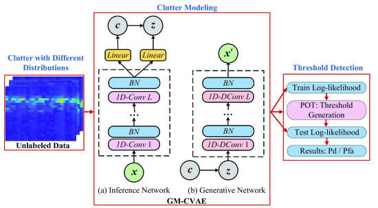
  • In order to solve the problem of complex and changeable clutter in the radar scanning range in the actual environment, we propose a GM-CVAE framework to realize refined modeling of clutter.
  • Considering that it is difficult to obtain the true labels of the data and the imbalance of clutter and target samples, we develop an unsupervised narrow-band radar target detection strategy based on reconstructed likelihood.
  • Experiments are used to evaluate our approach on simulated complex clutter datasets. These demonstrate the superiority of our method compared to the baselines.
The remaining parts of this paper are organized as follows. Section 2 presents the relevant preliminary knowledge. Section 3 describes the proposed method and the target detection strategy is presented in Section 4. Section 5 summarizes the numerical results and a general conclusion is presented in Section 6.

2. Preliminaries

In this section, we first introduce the clutter and target characteristics of the ground-based warning radar, respectively. Then, we provide a brief overview of the variational autoencoder, which is the basis of our work.

2.1. Ground Clutter Characteristics

Ground clutter is the main factor affecting the detection and tracking performance of the ground-based warning radar for low-altitude targets and ground targets. Essentially, ground clutter is the vector sum of echoes from many scatterers within the radar resolution cell. The clutter scattering phenomenon can be understood as a random process related to the random shape of the ground, which is usually described by the probability distribution model of clutter amplitude and clutter correlation model [43]. Many experimental facts have verified that for a low-resolution radar with a beam incident angle greater than 5° (antenna beam width greater than 2°, pulse width greater than 1 μs, the clutter amplitude distribution of sea clutter, ground clutter as well as meteorological clutter obeys the Rayleigh distribution. Therefore, this paper assumes that the ground clutter amplitude follows a Rayleigh distribution, the ground clutter power spectrum is described by a Gaussian function in which spectral center shift and spectral broadening are different, and partial relevant parameters in [44] are referred to for ground clutter simulation. In particular, the Rayleigh distribution is the distribution of the envelope of a Gaussian random signal passing through a narrow band linear system and needs to satisfy the following conditions: (1) The scatters within the radar irradiation unit are statistically independent. (2) The distance difference between the two scatters and the radar in the irradiation unit is much smaller than the scale of the irradiation unit, and the gain of the antenna in the unit is constant. (3) The number of scatterers is large and the signal is normally distributed according to the central limit theorem.

2.2. Target Characteristics

The primary task of the ground-based warning radar is to detect unknown targets as early as possible, determine their positions within the detection range as far as possible, and closely monitor the flying targets in the airspace. In order to satisfy the needs of long detection distance, ground-based warning radars generally work in lower frequency bands, mainly S and L frequency bands, and some work in the UHF frequency band, of course, VHF, and even HF frequency bands. The detection distance of ground-based warning radar is more than 350 km, even up to 550 km, but it does not have high requirements on the accuracy and resolution of the detection target. Generally, in low-resolution ground-based warning radar, the target imaged on the range-Doppler spectrum is a point-like target with a small scale, and usually does not cross range cells. Therefore, the radar target model considered in this paper is a point-like target that occupies only one range cell.

2.3. Variational Autoencoder

GM-CVAE is a variant of Variational Autoencoder (VAE) [45,46,47], which uses the Gaussian mixture model (GMM) as the prior of VAE latent space, extracts and expresses features of data through probability modeling. The biggest difference between GM-CVAE and VAE is that the former can handle complex multi-modal data, while the latter may not be able to approximate the original multi-modal data distribution well due to a single Gaussian distribution prior. Hence, a brief description of the variational autoencoder is necessary before introducing our methods.
VAE is a popular reconstruction probabilistic model which combines Bayesian inference with the autoencoder framework. The idea of VAE is that the distribution of complex data can be modeled by lower-dimensional latent variables or representations. In a regular VAE, ref. [47] first presents a computationally tractable method for training this model. Specifically, as shown in Figure 2, the prior distribution of the latent variables z , denotes p θ ( z ) , are often assumed to obey the unimodal Gaussian distribution, and generally for simplicity, p θ ( z ) N ( 0 , 1 ) , where p ( · ) is the probability distribution function and θ is the parameters of decoder. Through the encoder network with parameters ϕ , VAE learn posterior distribution q ϕ ( z | x ) so as to approximate the true posterior distribution p θ ( z | x ) . Then, it learns likelihood distribution p θ ( x | z ) so as to reconstruct the original input x through the decoder network with parameter θ . The better the z learned by the network, the more accurate the reconstruction will be. Given that the input data x is known and the latent variable z is unknown, we hope that two distributions q ϕ ( z | x ) and p θ ( z | x ) are as close as possible. Therefore, the following objective function [47] is obtained
m i n ϕ , θ D KL ( q ϕ ( z | x ) | | p θ ( z | x ) ) ,
where D KL stands for Kullback–Leibler divergence, which definition equation is D KL ( q ( x ) | | p ( x ) ) = q ( x ) log q ( x ) p ( x ) d x . It is mainly used to measure the similarity between two probability distributions. Next, through statistical derivation, the marginal log-likelihood of the input data x is obtained
log p ( x ) = D KL ( q ϕ ( z | x ) | | p θ ( z | x ) ) + L VAE ( ϕ , θ ; x ) ,
where
L VAE ( ϕ , θ ; x ) = E q ϕ ( z | x ) [ log p ( x , z ) ] E q ϕ ( z | x ) [ log q ϕ ( z | x ) ] ,
and L VAE ( ϕ , θ ; x ) is called the variational lower bound.
Since x is deterministic, log p ( x ) is a constant. Consequently, minimizing D KL term is equivalent to maximizing L VAE term according to Equation (2). Furthermore, the objective function of VAE can be rewritten as follows
m a x ϕ , θ L VAE ( ϕ , θ ; x )
Further derivation, Equation (4) can be rewritten as
L VAE ( ϕ , θ ; x ) = D KL ( q ϕ ( z | x ) | | p θ ( z ) ) + E q ϕ ( z | x ) [ log p θ ( x | z ) ]
The first term on the right side of equal sign in Equation (5) is the regularization term, which is used to minimize the difference between the posterior distribution q ϕ ( z | x ) and prior distribution p θ ( z ) ; the second term is the reconstruction term. The solution of L VAE ( ϕ , θ ; x ) is a maximum likelihood estimation process of input data x and can be solved by stochastic gradient descent (SGD) methods [47]. In addition, reconstruction loss is related to the input data form. If the input data is binary, binary cross entropy (BCE) can be used to approximate the loss; if the input data is continuous, the loss can be replaced by the mean square error (MSE).
However, regular VAEs often fail to approximate hidden layer distributions of complex data due to too simple prior assumptions. The idea behind our GM-CVAE is to use a Gaussian mixture distribution as a prior for the stochastic variable z , which depends on the categorical variable c . The prior of this variant is multi-modal and can learn more complex distributions than the unimodal prior. In this paper, we study a high-dimensional Gaussian mixture model to estimate the sample densities for target detection, which will be clear in next section.

3. Method

This section mainly discusses the Gaussian Mixture Variational Autoencoder with a one-dimensional Convolutional neural network (GM-CVAE), which is proposed to refine clutter modeling in an unsupervised manner to optimize target detection.

3.1. Overview of the Framework

The overall framework shown in Figure 3 comprises data pre-processing, the representation model and detection three modules.
The data pre-processing module firstly performs pulse compression on the radar echo data; then selects Moving Target Indication (MTI) or Adaptive Moving Target Indication (AMTI) for filtering processing according to static or moving clutter; after that, it utilizes Moving Target Detection (MTD) for coherent integration to obtain the range-Doppler spectrum (also called the R-D spectrum) and referring to [33,48], we take the modulus of the R-D spectrum; lastly, it performs a normalization operation to avoid numerical problems and speed up network convergence. we define the normalized R-D spectrum as X , X = [ x 1 , x 2 , , x N ] R M × N , where M and N represent the number of Doppler channel and range cell, respectively, and  R denotes the set of real number. The clutter data varies drastically in the spatial domain, and the assumption that data in the CUT and the reference cells are independent and identically distributed cannot be guaranteed. Therefore, x i R M × 1 , i = 1 , 2 , , N denotes the Doppler feature vector of the i-th range cell and makes it a sample in this paper. For the sake of description, we will ignore the subscript i for the rest of the discussion.
The difference between the data pre-processing process in this paper and the traditional radar signal processing process is the normalization step. Furthermore, we do not discuss a novel method of clutter suppression, which is beyond the scope of this paper. In the representation module, we propose a GM-CVAE to learn the complex structures and Doppler characteristics of clutter data. Its details will be covered in Section 3.2. Subsequently, target detection is performed based on the reconstruction results inferred from the model. The specific target detection method will be introduced in Section 4.

3.2. Network Architecture

As shown in Figure 4, GM-CVAE is a reconstruction-based model, including an inference network and a generative network. Next, we will introduce the two sub-networks, respectively.
Generative Network. It measures the likelihood of generating data instances given the latent variables. The generative model (as shown in Figure 4a) can factorize as
p θ ( x , z , c ) = p θ ( c , z ) p θ ( x | z ) = p θ ( c ) p θ ( z | c ) p θ ( x | z ) ,
and generate an observed sample x from the latent random variable z and latent discrete variable c , where θ is the network parameter. Specifically, we assign the form of the prior of the latent variable z as
z | c k = 1 K N z | μ k , diag ( σ k ) c k
where { μ , σ } = { μ k , σ k } k = 1 K represent the mean and variance parameters of multiple Gaussian distribution, which are obtained through the fully connected networks, respectively. K denotes the predefined number of components in the Gaussian mixture and diag ( · ) function constructs a diagonal matrix. c = c 1 , , c K T is an explicit latent variable associated with each x and is a one-hot vector subject to categorical prior distribution c Cat ( π ) with parameter π R + K × 1 . Thus, the latent variable z conditions on a different Gaussian distributed prior c , which indicates the diverse distribution characteristics of the input. Furthermore, by marginalizing z , the following equation can achieve
z c p θ ( c ) p θ ( z | c ) = k = 1 K π k N μ k , diag ( σ k )
Apparently, it is a mixture Gaussian distribution, which has higher representation power than a Gaussian distribution, so it is an ideal choice for characterizing the R-D spectrum characteristics of complex clutter.
Similar to [49], the generated distribution p θ ( x ^ | z ) is assigned as a Gaussian distribution and conditioned on both z , which can be expressed as
x ^ | z N ( μ x , σ x ) μ x = f w μ x z + b μ x σ x = f w σ x z + b σ x
where μ x and σ x denotes mean and variance parameters of the generated distribution. All w * -s, b * -s represent the weight parameters and bias parameters of the corresponding fully connected networks, respectively. f ( · ) is a nonlinear activation function, here we use LeakyReLU activation function and its expression is
LeakyReLU ( x ) = x , i f x 0 , α x , i f x < 0 ,
The value of α is 0.1 in our model.
Finally, to better generate the structures of data, the decoder performs the one-dimensional deconvolutional network as x = DCNN ( x ^ ) , where DCNN denotes the one-dimensional deconvolutional operation with trainable parameters D . As the deconvolution operation proceeds, the spatial resolution gradually increases, where the output of the final deconvolution layer is aimed at reconstructing the input x . Note that the constant change of model parameters during deep network training will cause the internal covariate shift [50], resulting in slow and inefficient network training. Hence, a BN layer is connected after the one-dimensional deconvolution layer in the deconvolution network to solve this problem.
Inference Network. It is a difficult problem to directly solve the generative model, i.e., finding maximum a posterior (MAP) of latent variables and maximum likelihood estimation (MLE) of parameters. In response to this issue, a new distribution q ϕ ( z , c | x ) is employed to approximate the true posterior distribution p θ ( z , c | x ) , which is drawn from specific class and parameterized by trainable parameter ϕ . Specifically, according to the mean-field theory approximation [51], the inference model (as shown in Figure 4b) can be factorized as
q ϕ ( z , c | x ) = q ϕ ( c | x ) q ϕ ( z | x , c )
In the inference network, for capturing the structural characteristics of input, a one-dimensional convolution network is conducted, i.e.,  x ¯ = CNN ( x ) , where CNN denotes the one-dimensional convolutional operation with parameters D ¯ . Similarly, a BN layer is connected after the one-dimensional convolution layer in Figure 4b. To increase the content covered by a convolutional kernel and the sparsity of the hidden units, a convolutional layer is usually followed by a pooling layer. However, the pooling layer that may reduce the resolution of the feature map is removed from the convolutional encoder, because the radar cross-sectional area of the target itself in the detection scene is small, the reflected energy is weak, and the scale of the target is small on the R-D spectrum.
After that, the parameter of the category distribution, that is, the indicator variable π , can be expressed as
π = softmax ( w π x ¯ + b π )
where w π and b π are the weight and bias parameters learned by the network, respectively. The  softmax function guarantees the non-negativity of probabilities. Then, we can obtain c by sampling π through Equation (14).
Finally, We parametrize variational factors with networks that output mean and diagonal covariance of variational distributions as well as assign their form as Gaussian posteriors
z | x ¯ , c N ( μ z , diag ( σ z ) ) μ z = f k = 1 K w μ z x ¯ + b μ z c k σ z = softplus k = 1 K w σ z x ¯ + b σ z c k
where f ( · ) denotes the LeakyReLU activation function, μ z and σ z are the mean and variance parameters of the latent variable z inferred by networks. Likewise, all w * -s, b * -s represent the weight parameters and bias parameters of the corresponding fully connected networks, respectively. softplus ( · ) = log ( 1 + exp ( · ) ) is to ensure original data non-negative after nonlinear transformation.
Note that, categorical variable c controls the structural prior of the latent variable z . Motivated by [47,52], we employ variational inference to learn c in GM-CVAE. However, c is a discrete variable, and the backpropagation algorithm is only applicable to differentiable layers, so it is not practical to directly optimize c . Hence, inspired by [53], we introduce the Gumbel-softmax trick to approximate the original categorical distribution c so that c is differentiable and learnable. Specifically, let the variational distribution q ϕ ( c ) = Gumbel softmax ( π ) , π R K × 1 , and 
c k = exp ( ( log π k + g k ) / λ ) l = 1 K exp ( ( log π l + g l ) / λ ) , k = 1 , , K , g k Gumbel ( 0 , 1 ) = log ( log ( ε k ) ) ,
where λ > 0 indicates the softmax temperature and controls the softness of softmax. ε k represents a standard uniform variable. When λ tends to 0, the samples from the Gumbel-softmax distribution become one-hot distribution, and the Gumbel-softmax distribution q ϕ ( c ) is consistent with the categorical distribution prior p θ ( c ) .
Furthermore, the same as regular VAE algorithms, we also use a Gaussian variational distribution q ϕ ( z ) to infer the posterior distribution of z in GM-CVAE, i.e.,
q ϕ ( z ) = N ( μ , σ 2 ) ,
where the two parameters μ and σ are transformed by the inference network, and sampling from the latent variables can be achieved by [47]
z = μ + σ ϵ ,
thus ensuring normal execution of the back-propagation algorithm. Herein, ϵ is a vector with all its entries drawn independently from the standard Gaussian distribution, and “⊙” denotes element-wise product.
The goal of GM-CVAE is to find a better stochastic latent representation z for data x . For large and complex terrain scenes, it is difficult to accurately describe the entire ground clutter area with one distribution model, and even the same terrain scene obeys different distributions under the influence of different time and climatic conditions. Different clutter backgrounds obey different probability distributions, resulting in the existence of multiple normal modes in the data center. Therefore, it is an excellent choice for the prior of z to follow the mixture Gaussian distribution.
The generative network and inference network are trained together to approximate the true posterior distribution. Details are described below.

3.3. Offline Training Process

GM-CVAE model can be trained by maximizing the evidence of lower bound (ELBO) [54] on the log-likelihood of input data, L GM CVAE ( ϕ , θ ; x ) ,
L GM CVAE ( ϕ , θ ; x ) = E q ϕ ( z , c | x ) log p θ ( x , z , c ) q ϕ ( z , c | x )
Combine Equations (6) and (11), and rewrite Equation (17)
L GM CVAE ( ϕ , θ ; x ) = E q ϕ ( z , c | x ) log p θ ( x , z , c ) q ϕ ( z , c | x ) = E q ϕ ( z , c | x ) log p θ ( c ) q ϕ ( c | x ) + log p θ ( z | c ) q ϕ ( z | x , c ) + log p θ ( x | z ) = E q ϕ ( z , c | x ) log p θ ( x | z ) D KL q ϕ ( c | x ) | | p θ ( c ) D KL q ϕ ( z | x , c ) | | p θ ( z | c )
In Equation (18), the first term is the expected log-likelihood of the data x , which aims to guarantee the reconstruction capacity of the generative model. The second term is the regularization between the prior p θ ( c ) and posterior q ϕ ( c | x ) of the categorical variable c that constrains the two distributions as close as possible. The third term represents the regularization between the actual posterior p θ ( z | c ) and approximate posterior q ϕ ( z | x , c ) of the latent variable z . The closer the prior and posterior distributions are, the smaller the regularization value. Specifically, since c is a discrete variable, the second term in Equation (18) can be written as
D KL q ϕ ( c | x ) | | p θ ( c ) = k = 1 K q ϕ ( c k = 1 | x ) log q ϕ ( c k = 1 | x ) p θ ( c k = 1 ) = k = 1 K q ϕ ( c k = 1 | x ) log ( q ϕ ( c k = 1 | x ) ) log 1 K
As we assign the prior of latent variables as mixture Gaussian distribution, the KL divergence of the third term in Equation (18) can be calculated as
D KL q ϕ ( z | x , c ) | | p θ ( z | c ) = k = 1 K c k q ϕ z | x , c log q ϕ ( z | x , c ) N μ k , σ k = k = 1 K c k D KL q ϕ ( z | x , c ) | | N μ k , σ k
Moreover, the analytical expression of KL divergence between two Gaussian distributions is
D KL N ( μ 1 , diag ( σ 1 ) ) | | N ( μ 2 , diag ( σ 2 ) ) = 1 2 log σ 1 σ 2 d + σ 2 1 σ 1 + ( μ 1 μ 2 ) T diag ( σ 2 1 ) ( μ 1 μ 2 ) ,
where d is the dimension of variables; diag ( · ) function constructs a diagonal matrix and ( · ) T denotes a transpose operation. The analytical KL divergence expressions in Equations (19)–(21), and the reparameterization tricks of Gumbel-softmax in Equation (14) and Gaussian distribution in Equation (16) allow the gradients of ELBO with respect to parameters in the inference network to be accurately evaluated.
Algorithm 1 summarizes the GM-CVAE training algorithm under complex clutter background in an unsupervised learning fashion.
Algorithm 1: GM-CVAE Training Algorithm
input: The pre-processed R-D spectrum training set X train = { x i } i = 1 N train ; number of components K; batch-size M.
output: The encoder parameters ϕ and the decoder parameters θ ; reconstruction probability vector for all samples s train (see Equation (22));
θ , ϕ  ← Initialize parameters.
repeat
  Select a mini-batch training subset { x n } n = 1 M randomly;
  Draw random noise { ε } n = 1 M from uniform distribution for generating samples { c } n = 1 M according to Equation (14);
  Draw random noise { ϵ } n = 1 M from normal distribution for generating latent variable { z } n = 1 M according Equation (16);
  Calculate L GM CVAE ( ϕ , θ ; x ) according to Equations (18)–(21), and update parameters of the two sub-nets jointly;
until convergence
return model parameters ϕ and θ , as well as s train .

4. Target Detection Strategy

The GM-CVAE model learns the network parameters to capture the normal patterns of clutter samples after offline training. Now based on the difference between clutter and target echo in Doppler feature space, we can ensure whether the input sample x is a target by utilizing the trained model. The reconstruction probability in the GM-CVAE model indicates its reconstruction difficulty [51]: the lower the reconstruction probability value, the more difficult it is to be accurately reconstructed. For a sample with a target, it will be difficult to be reconstructed accurately, and its reconstruction probability is often lower than that of a sample only with clutter [55]. Inspired by [56], we decided to take the reconstruction probability of x as the final score, denoted as s, and compare it with threshold t to determine whether the observed sample is a target. The calculation formula is as follows
s = E q ϕ ( z , c | x ) log p θ ( x | z )
If the final score s is less than threshold t, observed sample x is determined as a target; otherwise, it will be judged as a pure clutter sample. The threshold t is learned automatically in the GM-CVAE model. Extreme Value Theory (EVT) takes extreme data as the research object, and infers the distribution of extreme data that may be observed without any distribution based on the original data. The second theorem in EVT, the Peaks-Over-Threshold (POT) [57] model, is based on the generalized Pareto distribution to model the distribution of all observed data that exceeds a sufficiently large threshold to study the tail characteristics of the distribution. POT demonstrates excellent performance in threshold tuning, so we apply the adjusted POT method to help choose the threshold t for GM-CVAE. Algorithm 2 describes the process of threshold detection.
Algorithm 2: GM-CVAE Detection Algorithm
input: The pre-processed R-D spectrum test set X test = { x i } i = 1 N test ;
output: reconstruction probability vector for all samples s test (see Equation (22)) and labels y .
ϕ , θ , s train  ← Trained GM-CVAE network.
 Similar to the loop body of Algorithm 1, reconstruction probability vector s test is obtained;
 Feed s train as the initial threshold to the POT algorithm to generate the final threshold vector t ;
 Element-wise comparison of s test and t :
if s test ( i ) < t ( i ) , then then
   x i is a target, label y i = 1
else
   x i is a clutter, label y i = 0
end if

5. Numerical Examples

In this section, we first introduce our experiment setup in Section 5.1, including experiment data, evaluation metrics, compared baselines, model hyper-parameters and hardware platform. We then evaluate and compare the performances of GM-CVAE and baselines in different clutter scenes in Section 5.2. Finally, we qualitatively analyze the proposed method in Section 5.3.

5.1. Experiment Setup

Experiment Data. In the simulation, the linear frequency modulated signal is chosen for the waveform of the ground-based warning radar, which operates at a wavelength of 0.23 m, a bandwidth of 2 MHz, an azimuth beam width of 2 ° , a pulse width of 0.15 ms, a pulse repetition period of 2.37 ms, a sampling frequency of 4 MHz, and 23 coherent pulses in one CPI. In order to fit different terrains with different data distributions, three types of clutter are designed for simulating complex clutter scenes, and Figure 5 shows their R-D spectrum. The x-axis represents 50 range cells of radar, and the y-axis represents the normalized Doppler frequency, which can be converted to the corresponding radial velocity. The red solid box in the figure represents the primary clutter area, and targets will locate in it if data is not dealt with MTI or AMTI in the data pre-processing stage. The green dotted box represents the secondary clutter area and targets will fall in it if MTI or AMTI is conducted in the data pre-processing stage. Figure 6a demonstrates the Doppler characteristics of three types of clutter. The center frequency and clutter spectrum width of three types of clutter are different, Type-2 is static clutter, while Type-1 and Type-3 are moving clutter with different speeds. Figure 6b exhibits the power intensity of three types of clutter partial range cells. It can be seen that the three types of clutter fluctuate violently in space, and it is difficult for the samples to satisfy the conditions of independent and identical distribution. Therefore, combined with the characteristics of the target data, we use each Doppler vector in the R-D spectrum as sample data, and 1D-CNN is used to extract sample features in our GM-CVAE. In the experiment, we have 2400 clutter instances in total and divide the dataset into two parts: the former 2000 for training and the latter 400 for testing. The ratios of target instances in the testing set is 0.05.
Evaluation Metrics. We mainly employ two performance metrics to evaluate GM-CVAE and other baseline methods: detection probability (denoted as P d ) and the false alarm rate (denoted as P f a ). They can be shown as following [35]
P d = Recall = TP TP + FN P f a = 1 Precision = FP TP + FP
Compared Baselines. To demonstrate the effectiveness of GM-CVAE, one-dimensional convolutional VAE (CVAE), classical CA-CFAR [3], GO-CFAR [7] and OS-CFAR [9] detectors as well as adaptive detectors, i.e., adaptive normalized matched filter (ANMF) [19] and ASD [27] are chosen as baselines. For ASD detector, we consider the rank-1 case (that is, the subspace signal model is represented as the product of the target amplitude and the steering vector). In other words, the performance of GM-CVAE is compared with the five classical detection methods and CVAE uses a simple Gaussian prior to learn the latent spatial distribution of the data.
Hyper-parameters. In our experiments, GM-CVAE is implemented based on Pytorch. The hyper-parameters of GM-CVAE are set empirically in our experiments as follows. Both the convolutional and deconvolutional layer L = 2, the kernel sizes and strides of which are { 3 × 1 , 3 × 1 } and { 2 × 1 , 2 × 1 } , respectively. The dimension of z -space is 5 empirically and the components of categorical-space are related to the number of clutter types, and the value set is from { 1 , 2 , 3 } . For the adjusted POT method, the low quantile = 0.2 and q = 10 4 [57]. GM-CVAE is trained with Adam optimizer [58], with a learning rate of 0.0005 . We run 50 epochs for training, and the batch size is 64. More studies about the choice of hyper-parameters will be discussed later.
Hardware Platform Our experiments are conducted on a host with Intel(R) Core(TM) i7-10700 CPU @ 2.90GHz accelerated by NVIDIA RTX 3080, with 10 GB VRAM of the graphic card.

5.2. Performance Comparison

In the range-Doppler domain, clutter or targets with different velocities occupy different Doppler cells, which is an important feature to effectively distinguish signals of different velocities. The Doppler frequency of the slow target is extremely low, and it often overlaps with the Doppler of low-frequency clutter. At this time, the target is submerged in the strong clutter, and feature extraction is difficult, thereby reducing the detection performance. During data pre-processing, the MTI filter can suppress the static zero-frequency ground clutter well, and has better detection performance for higher-speed moving targets, such as the echo of target 2 in Figure 7. However, when detecting a slow-moving target with a lower Doppler frequency, the MTI filter also greatly suppresses the moving target near the zero frequency, such as the attenuated target 1 echo in Figure 7. Likewise, the AMTI filter can better suppress motion clutter, but it can also suppress targets with similar clutter Doppler frequencies. To this end, two scenarios in target detection are considered, one is to employ the MTI or AMTI filter during data pre-processing, and the position of the target avoids the filter notch in the Doppler dimension (see the green dotted box in Figure 5) and is random in the range dimension; another, is to not utilize MTI or AMTI filter during data pre-processing, and the target is added to primary clutter area (See the red solid box in Figure 5).

5.2.1. Data Pre-Processing with MTI or AMTI

The size of the reference window with the aforementioned traditional detectors is 24, and the length of the guard cell is 2. A total of 10 4 Monte Carlo trials are performed. The selection of order k in OS-CFAR is 14 and the target obeys the Swerling type-0/5 distribution. Note that the comparison between network methods and other detectors: the actual false alarm rate of the test set is used as the constant false alarm rate of CA-CFAR, GO-CFAR, OS-CFAR, ANMF and ASD methods after the network training is completed, and then detection probability of the two methods is compared. If the actual false alarm rate in network methods is zero, the constant false alarm rate in the traditional methods is set to 10 3 .
Performances in Single-clutter Scene. Taking Type-2 as an example, the detection probabilities of GM-CVAE, CVAE and the five traditional methods versus Signal to Noise Ratio (SNR) are presented in Figure 8a,b, respectively, where the noise power is about 59.3 dB. The actual false alarm rate of GM-CVAE, CVAE and the five traditional detection methods versus SNR are presented in Figure 8d,e, respectively. Figure 8c,f compare the detection and false alarm performance of GM-CVAE and CVAE, respectively. Specifically, GM-CVAE is far superior to CA-CFAR, GO-CFAR and OS-CFAR methods in terms of detection performance under low SNR conditions. The detection performance of ANMF and ASD in the single clutter scene is similar, and compared with the two detectors, our proposed GM-CVAE has a performance improvement of about 3 dB. Since ANMF is a coherent accumulator, it can improve the accumulation gain by accumulating multiple samples, and thus has better detection performance than the three CFAR detectors. From the perspective of false alarm, the five traditional detection methods are slightly higher than the GM-CVAE method, in which the false alarm value fluctuates reasonably. Similar conclusions occur for CVAE and CA-CFAR, GO-CFAR, OS-CFAR, ANMF and ASD methods. Furthermore, compared with Figure 8c,f, GM-CVAE performs slightly better than CVAE under single clutter background, indicating that GMM prior extracts more information than single Gaussian prior.
Performances in Complex-clutter Scene. To simulate the complexity of multiple clutter in radar irradiation area, different types of clutter regions are spliced according to the range dimension. The complex scene is shown in Figure 9, where the three types of clutter are concatenated in equal proportions. The noise powers of Type-1, Type-2 and Type-3 clutter are 56.0 dB, 59.3 dB, and 64.7 dB, respectively. Figure 10 exhibits the detection performances and actual false alarm rates under complex clutter scene.
GM-CVAE and CVAE in Figure 10a,b provide excellent detection performances while CA-CFAR, GO-CFAR and OS-CFAR detection methods suffer a performance degradation owing to the clutter edge effect. Compared with ANMF (or ASD) and GM-CVAE, the latter is improved by about 9 dB. This is because ANMF and ASD detectors rely on clutter covariance matrix estimation. When the clutter is heterogeneously distributed, it is difficult to have a sufficient number of i.i.d. training samples. Furthermore, P f a of CA-CFAR, GO-CFAR and OS-CFAR increases so significantly that it can no longer maintain the constant false alarm rate, our GM-CVAE continues to work robustly yet. Compared with the detection performances of GM-CVAE and CVAE methods in Figure 8c and Figure 10c, it is evident from the result of comparison that the more complex the clutter distribution is, the more significant the P d improvement of the proposed method is, i.e., the performance of the two methods in a single-clutter scene is close, while P d is improved by about 2.5 dB under the complex clutter background. This phenomenon indicates that for complex data distribution, GM-CVAE can learn more abundant representational features than CVAE, realizes refined modeling of clutter, and reflects the superiority of GMM prior.
The SNR improvements of the proposed method under different clutter scenes when compared with the CA-CFAR method are summarized in Table 1. CVAE, OS-CFAR, GO-CFAR, ANMF and ASD methods are also considered for better comparison. Since the constant false alarm parameter in the five traditional methods come from the actual false alarm rate of the network method, CVAE and GM-CVAE are compared with CA-CFAR, respectively. Herein, we set the required SNR of the CA-CFAR method to satisfy the reference. In addition to the two clutter scenarios given above, Table 1 also quantitatively analyzes the SNR enhancement of the other two complex scenarios. The statistic in Table 1 demonstrates that our GM-CVAE provides excellent detection performances compared to traditional CA-CFAR, GO-CFAR, OS-CFAR, ANMF and ASD detection methods, both in single-clutter and complex-clutter scenes. Moreover, with the diversification of clutter distribution, the improvement of GM-CVAE detection performance is more evident.

5.2.2. Data Pre-Processing without MTI or AMTI

Performances in Single-clutter Scene. In order to contrast with the previous experiments, we still choose Type-2 clutter as an example, the size of the reference window with the three CFAR methods is 24, and the length of the guard cell is 2. The selection of order k in OS-CFAR is 15 and the noise power is 52.4 dB. The comparison results of different methods are shown in Figure 11. The five traditional detectors suffer a performance degradation owing to the absence of clutter suppression compared to GM-CVAE (Figure 11a,d) and CVAE (Figure 11b,e). It also can be seen that our GM-CVAE increases by about 2 dB compared with that of CVAE under the same P d (Figure 11c), the P f a drops significantly at lower SNRs concurrently. This further verifies that the proposed GM-CVAE method can more effectively model the distribution of data in harsh clutter environments. In addition, regardless of the network methods or the traditional CFAR methods, the detection performance drops significantly compared to Figure 8, and the traditional CFAR methods almost completely fail at this time. This indicates that when the target velocity is extremely low, it will be seriously affected by clutter, and it is extremely difficult to extract Doppler information.
Performances in Complex-clutter Scene. The selection of order k in OS-CFAR is 16 and the noise power of the three regions is 53.8 dB, 52.4 dB, and 59.4 dB, respectively. Likewise, Figure 12 exhibits the performance curves under the background of complex clutter. With the dual effects of clutter filtering-free and clutter edge, CA-CFAR, GO-CFAR, OS-CFAR, ANMF and ASD detection methods work poorly compared with CVAE and GM-CVAE methods, and CA-CFAR has the worst effect. Compared to the three CFAR detectors, ANMF and ASD achieve slightly higher detection gains due to the coherent accumulation of samples. Moreover, the five traditional detectors need to sacrifice high SNR to detect the target. P f a of the three CFAR methods multiplies approximately compared with CVAE and GM-CVAE methods, and the order k needs to be chosen carefully. In addition, our proposed GM-CVAE method in this scenario continues to work robustly, with higher detection probability and lower false alarm rate than CVAE. This further explains that the isotropic distribution of simple Gaussian in VAE fails to model the intrinsic multimodality of high dimensional data. In conclusion, our GM-CVAE method does have advantages for modeling complex clutter, and it can improve the performance of radar target detection.

5.3. Qualitative Analysis

The Influence of Model Parameters. In this part, we discuss the sensitivity of model parameters, namely the dimension of hidden stochastic variables (i.e., z ). The reason we do not talk about the number of components of Gaussian mixture c is because the number of clutter types is assumed to be exactly known in each experiment.
GM-CVAE is a reconstruction-based model. For an input observation, GM-CVAE compresses it to a low dimension z -space representation and then uses the representation to reconstruct it. That is to say, in this process, the key features in the original data are retained and finally used for reconstruction; some unimportant features are eliminated. Therefore, if the dimension of the latent space z is too low, it means that there are too few key features, and it is easy to lose mode which will lead to the under-fitting of the model; if the dimension of z is too high, it means that more rare features will contribute to the model, making the search space larger and more saddle points present. This makes the learning rate of the model more slowly, and in addition, it will take up too much video memory. Based on this, when SNR = 11 dB, we set the dimension of z ranges from 2 to 8 in the experiment, observe its impact on the detection performance, and choose the most suitable dimension. It can be seen from Figure 13 that the detection probability P d increases significantly when the dimension of z increases from 2 to 5. This means that adding key features improves the representation ability of the model. When the dimension of z is 5, the detection probability is the highest, which means that the key features retained at this time are enough to represent the original data. When we continue to increase the dimension of z , it will not bring significant improvement, but may reduce the performance of the model due to the increase in the search space and the increase in saddle points. Hence, the dimension of z is set to 5 in this paper.
Visualization of z -space Representations. To illustrate that our model can fine model complex clutter distributions, here we visualize the 2D embedding in the original data domain and z -latent space on the GM-CVAE model for complex clutter scene using t-distributed stochastic neighborhood embedding (t-SNE) [59] method in Figure 14. Each dot in the figure indicates the latent variable of the observation vector, and each color represents a cluster group. The class boundaries of the training samples are blurred in the original data domain according to Figure 14a,c, while samples are separable in z -latent space and work well according to Figure 14b,d. This result indicates that our model can represent different clutter features with the mixture distributed latent variables, thus verifying that GM-CVAE can refine modeling.
The number of components of the Gaussian mixture c in the experiments is consistent with the set number of clutter types. If the number of components of Gaussian mixture c is changed in a multiple, i.e., more than one Gaussian component is used for each cluster to approximate the distribution, and the detection performance in single clutter and complex clutter scenes is considered, the results are shown in Figure 15a. The horizontal axis in Figure 15a represents the multiple expansion of the original Gaussian mixture component number. It can be seen that the detection performance has improved in both scenes, but the improvement effect is minimal. The analysis is as follows: objects in a cluster are similar or related to each other, and objects in different clusters are dissimilar or irrelevant. The more similar within clusters and the greater the gap between clusters, the better the effect. However, as shown in Figure 14b,d, our three kinds of data have a large distance in the z latent space itself. Even if it is divided into more clusters (as shown in Figure 15b, 6 clusters), the distance among the clusters does not widen each other. So the performance gain is quite limited.
Furthermore, to show intuitively the efficiency of our mixture distributed latent variable, four case studies of GM-CVAE are shown in Figure 16. Figure 16a shows the sequence of test samples in the background of single-clutter filtered by MTI or AMTI and Figure 16c displays the corresponding log-likelihood score. It can be seen from Figure 16a,c that even if some targets are similar to the clutter distribution, our model is still able to correctly learn the distribution of the clutter and gives the target points a lower log-likelihood. A similar conclusion can be observed in Figure 16b,d. In addition, the target in the red circle in Figure 16b is submerged in the clutter, but the corresponding score exhibits a clear peak, which further validates the superiority of our model in capturing complex clutter features. In Figure 16e,f, the phenomenon of some targets submerged in clutter is more prominent, but the GM-CVAE score remains stable. For the complex-clutter scenes in Figure 16b,f, GM-CVAE can model the non-stationary input assigned into different cluster groups with different parameters, thus leading to a more stable score, while it exhibits considerable spikes in the regions of targets. Consequently, GM-CVE is robust and effective for modeling complex clutter.

6. Conclusions

Traditional detection methods often face the problem of model mismatch under complex clutter backgrounds. Moreover, it is difficult to obtain target data and labels, which makes supervised deep learning methods difficult to implement. To solve this problem, We propose an unsupervised target detection approach (GM-CVAE). GM-CVAE assigns its latent variables into a mixture Gaussian distribution and thus it can model the normal patterns of clutter samples finely by learning their low-dimensional representations, fully capturing Doppler shape features and various data distributions. Moreover, GM-CVAE provides an intuitive and effective way to detect targets based on reconstruction probability. The extensive experimental results demonstrate that GM-CVAE outperforms the traditional detection approaches and CVAE model with single Gaussian as prior in terms of detection probability and the false alarm rate, and show the superiority of one model that fits a great variety of clutter distributions. In addition, our model also achieves effective detection of slow targets in complex clutter backgrounds without sample labels. Although this work adopts simulated data for training, we believe that it has promising potential to apply unsupervised deep learning to radar target detection on complex clutter data. In addition, we expect to obtain sufficient training data with multiple distributions from the radar system which will definitely prompt the detection model to be more convincing. In the future, we will try to extend and evaluate our model with real-world radar data. Other signal features will be analyzed to improve the model performance to adapt complex clutter environment.

Author Contributions

Conceptualization, X.L. and B.C.; methodology, X.L., B.C. and W.C.; data curation, X.L. and B.C.; formal analysis, X.L. and W.C.; writing—original draft preparation, X.L.; visualization, X.L. and W.C.; supervision, B.C., P.W. and H.L.; funding acquisition, B.C. and H.L. All authors have read and agreed to the published version of the manuscript.

Funding

This work was supported in part by the National Natural Science Foundation of China under Grant U21B2006 and Grant 61771361; in part by Shaanxi Youth Innovation Team Project; in part by the 111 Project under Grant B18039; and in part by the Thousand Young Talent Program of China.

Data Availability Statement

Not applicable.

Acknowledgments

B. Chen acknowledges the support of NSFC (U21B2006 and 61771361), Shaanxi Youth Innovation Team Project, the 111 Project (No. B18039) and the Program for Oversea Talent by Chinese Central Government. W. Chen acknowledges the support of National Key Lab Fund project.

Conflicts of Interest

The authors declare no conflict of interest.

Abbreviations

The following abbreviations are used in this manuscript:
ANMFAdaptive normalized matched filter
ASDAdaptive subspace detector
CFARConstant false alarm rate
CA-CFARCell-averaging CFAR
GO-CFARThe greatest of selection CFAR
OS-CFARThe order statistic CFAR
CUTCell under test
CNNConvolutional neural network
GMMGaussian mixture model
VAEVariational autoencoder
CVAEVariational autoencoder with 1D-CNN
GM-CVAEGaussian mixture variational autoencoder with 1D-CNN
EVTExtreme value theory
POTPeaks over threshold

References

  1. Yan, J.; Liu, H.; Pu, W.; Liu, H.; Liu, Z.; Bao, Z. Joint Threshold Adjustment and Power Allocation for Cognitive Target Tracking in Asynchronous Radar Network. IEEE Trans. Signal Process. 2017, 65, 3094–3106. [Google Scholar] [CrossRef]
  2. Zhang, H.; Liu, W.; Shi, J.; Fei, T.; Zong, B. Joint Detection Threshold Optimization and Illumination Time Allocation Strategy for Cognitive Tracking in a Networked Radar System. IEEE Trans. Signal Proc. 2022, 126, 1–15. [Google Scholar] [CrossRef]
  3. Finn, H.M. Adaptive Detection Mode with Threshold Control as A Function of Spatially Sampled Clutter Level Estimates. RCA Rev. 1968, 29, 414–465. [Google Scholar] [CrossRef]
  4. Weiss, M. Analysis of Some Modified Cell-Averaging CFAR Processors in Multiple-target Situations. IEEE Trans. Aeros. Electron. Syst. 1982, 18, 102–114. [Google Scholar] [CrossRef]
  5. Gandhi, P.; Kassam, S. Analysis of CFAR Processors in Nonhomogeneous Background. IEEE Trans. Aerosp. Electron. Syst. 1988, 24, 427–445. [Google Scholar] [CrossRef]
  6. Hansen, V.G. Constant False Alarm Rate Processing in Search Radars. In Proceedings of the IEE Conference on Radar-Present and Future, London, UK, 23–25 October 1973; pp. 325–332. [Google Scholar]
  7. Hansen, V.G.; Sawyers, J.H. Detectability Loss Due to “Greatest Of” Selection in a Cell-Averaging CFAR. IEEE Trans. Aeros. Electron. Syst. 1980, 16, 115–118. [Google Scholar] [CrossRef]
  8. Rohling, H. Radar CFAR Thresholding in Clutter and Multiple Target Situations. IEEE Trans. Aerosp. Electron. Syst. 1983, 19, 608–621. [Google Scholar] [CrossRef]
  9. Elias Fusté, A.; de Mercado, G.G.; de los Reyes, E. Analysis of Some Modified Ordered Statistic CFAR: OSGO and OSSO CFAR. IEEE Trans. Aerosp. Electron. Syst. 1990, 26, 197–202. [Google Scholar] [CrossRef]
  10. Pourmottaghi, A.; Taban, M.; Gazor, S. A CFAR Detector in A Nonhomogenous Weibull Clutter. IEEE Trans. Aerosp. Electron. Syst. 2012, 48, 1747–1758. [Google Scholar] [CrossRef]
  11. Zhang, X.; Zhang, R.; Sheng, W.; Ma, X.; Han, Y.; Cui, J.; Kong, F. Intelligent CFAR Detector for Non-homogeneous Weibull Clutter Environment Based on Skewness. In Proceedings of the 2018 IEEE Radar Conference (RadarConf18), Oklahoma City, OK, USA, 23–27 April 2018. [Google Scholar] [CrossRef]
  12. Roy, L.; Kumar, R. Accurate K-distributed Clutter Model for Scanning Radar Application. IET Radar Sonar Navig. 2010, 4, 158–167. [Google Scholar] [CrossRef]
  13. Yang, Y.; Xiao, S.p.; Feng, D.j.; Zhang, W.m. Modelling and Simulation of Spatial-temporal Correlated K Distributed Clutter for Coherent Radar Seeker. IET Radar Sonar Navig. 2014, 8, 1–8. [Google Scholar] [CrossRef]
  14. Conte, E.; Longo, M. Characterisation of Radar Clutter as A Spherically Invariant Random Process. IEE Proc. Part F 1987, 134, 191–197. [Google Scholar] [CrossRef]
  15. Sangston, K.J.; Gini, F.; Greco, M.V.; Farina, A. Structures for Radar Detection in Compound Gaussian Clutter. IEEE Trans. Aerosp. Electron. Syst. 1999, 35, 445–458. [Google Scholar] [CrossRef]
  16. Gini, F.; Farina, A. Vector Subspace Detection in Compound-Gaussian Clutter. Part I: Survey and New Results. IEEE Trans. Aerosp. Electron. Syst. 2002, 38, 1295–1311. [Google Scholar] [CrossRef]
  17. Gini, F.; Farina, A.; Montanari, M. Vector Subspace Detection in Compound-Gaussian Clutter. Part II: Performance Analysis. IEEE Trans. Aerosp. Electron. Syst. 2002, 38, 1312–1323. [Google Scholar] [CrossRef]
  18. Xu, S.W.; Shui, P.L.; Cao, Y.H. Adaptive Range-spread Maneuvering Target Detection in Compound-Gaussian Clutter. Digit. Signal Process. 2015, 36, 46–56. [Google Scholar] [CrossRef]
  19. Conte, E.; Lops, M.; Ricci, G. Adaptive Detection Schemes in Compound-Gaussian Clutter. IEEE Trans. Aerosp. Electron. Syst. 1998, 34, 1058–1069. [Google Scholar] [CrossRef]
  20. Chen, B.; Varshney, P.K.; Michels, J.H. Adaptive CFAR Detection for Clutter-edge Heterogeneity using Bayesian Inference. IEEE Trans. Aerosp. Electron. Syst. 2003, 39, 1462–1470. [Google Scholar] [CrossRef]
  21. Zaimbashi, A. An Adaptive Cell Averaging-based CFAR Detector for Interfering Targets and Clutter-edge Situations. Digit. Signal Process. 2014, 31, 59–68. [Google Scholar] [CrossRef]
  22. Doyuran, U.C.; Tanik, Y. Expectation Maximization-based Detection in Range-heterogeneous Weibull Clutter. IEEE Trans. Aerosp. Electron. Syst. 2014, 50, 3156–3166. [Google Scholar] [CrossRef]
  23. Meng, X. Rank Sum Nonparametric CFAR Detector in Nonhomogeneous Background. IEEE Trans. Aerosp. Electron. Syst. 2020, 57, 397–403. [Google Scholar] [CrossRef]
  24. Hua, X.; Ono, Y.; Peng, L.; Xu, Y. Unsupervised Learning Discriminative MIG Detectors in Nonhomogeneous Clutter. IEEE Trans. Commun. 2022, 70, 4107–4120. [Google Scholar] [CrossRef]
  25. Aubry, A.; De Maio, A.; Pallotta, L.; Farina, A. Covariance Matrix Estimation via Geometric Barycenters and Its Application to Radar Training Data Selection. IET Radar Sonar Navig. 2013, 7, 600–614. [Google Scholar] [CrossRef]
  26. Wang, Z.; Li, G.; Chen, H. Adaptive Persymmetric Subspace Detectors in the Partially Homogeneous Environment. IEEE Trans. Signal Process. 2020, 68, 5178–5187. [Google Scholar] [CrossRef]
  27. Kraut, S.; Scharf, L.; McWhorter, L. Adaptive Subspace Detectors. IEEE Trans. Signal Process. 2001, 49, 1–16. [Google Scholar] [CrossRef]
  28. Liu, J.; Sun, S.; Liu, W. One-Step Persymmetric GLRT for Subspace Signals. IEEE Trans. Signal Process. 2019, 67, 3639–3648. [Google Scholar] [CrossRef]
  29. Bidart, R.; Wong, A. Affine Variational Autoencoders. In Proceedings of the International Conference on Image Analysis and Recognition, Waterloo, ON, Canada, 27–29 August 2019; pp. 461–472. [Google Scholar]
  30. Cai, F.; Ozdagli, A.I.; Koutsoukos, X. Detection of Dataset Shifts in Learning-Enabled Cyber-Physical Systems using Variational Autoencoder for Regression. In Proceedings of the 2021 4th IEEE International Conference on Industrial Cyber-Physical Systems (ICPS), Victoria, BC, Canada, 10–12 May 2021; pp. 104–111. [Google Scholar] [CrossRef]
  31. Liu, N.; Xu, Y.; Ding, H.; Xue, Y.; Guan, J. High-dimensional Feature Extraction of Sea Clutter and Target Signal for Intelligent Maritime Monitoring Network. Comput. Commun. 2019, 147, 76–84. [Google Scholar] [CrossRef]
  32. Lopez-Risueno, G.; Grajal, J.; Diaz-Oliver, R. Target Detection in Sea Clutter using Convolutional Neural Networks. In Proceedings of the 2003 IEEE Radar Conference (Cat. No. 03CH37474), Huntsville, AL, USA, 5–8 May 2003; pp. 321–328. [Google Scholar] [CrossRef]
  33. Jing, H.; Cheng, Y.; Wu, H.; Wang, H. Adaptive Network Detector for Radar Target in Changing Scenes. Remote Sens. 2021, 13, 3743. [Google Scholar] [CrossRef]
  34. Wang, L.; Tang, J.; Liao, Q. A Study on Radar Target Detection Based on Deep Neural Networks. IEEE Sens. Lett. 2019, 3, 1–4. [Google Scholar] [CrossRef]
  35. Xie, Y.; Tang, J.; Wang, L. Radar Target Detection using Convolutional Neutral Network in Clutter. In Proceedings of the 2019 IEEE International Conference on Signal, Information and Data Processing (ICSIDP), Chongqing, China, 11–13 December 2019; pp. 1–6. [Google Scholar] [CrossRef]
  36. Kan, M.; Shan, S.; Chen, X. Bi-shifting Auto-encoder for Unsupervised Domain Adaptation. In Proceedings of the IEEE International Conference on Computer Vision, Santiago, Chile, 7–13 December 2015; pp. 3846–3854. [Google Scholar] [CrossRef]
  37. Rostami, M. Lifelong Domain Adaptation via Consolidated Internal Distribution. Adv. Neural Inf. Process. Syst. 2021, 34, 11172–11183. [Google Scholar] [CrossRef]
  38. Lasloum, T.; Alhichri, H.; Bazi, Y.; Alajlan, N. SSDAN: Multi-Source Semi-Supervised Domain Adaptation Network for Remote Sensing Scene Classification. Remote Sens. 2021, 13, 3861. [Google Scholar] [CrossRef]
  39. Zhang, Y.; Shen, D.; Wang, G.; Gan, Z.; Henao, R.; Carin, L. Deconvolutional paragraph representation learning. arXiv 2017, arXiv:1708.04729. [Google Scholar]
  40. Xie, R.; Sun, Z.; Wang, H.; Li, P.; Rui, Y.; Wang, L.; Bian, C. Low-Resolution Ground Surveillance Radar Target Classification Based on 1D-CNN. In Proceedings of the Eleventh International Conference on Signal Processing Systems, Chengdu, China, 15–17 November 2019; Volume 11384, pp. 199–204. [Google Scholar] [CrossRef]
  41. Xie, R.; Dong, B.; Li, P.; Rui, Y.; Wang, X.; Wei, J. Automatic Target Recognition Method For Low-Resolution Ground Surveillance Radar Based on 1D-CNN. In Proceedings of the Twelfth International Conference on Signal Processing Systems, Xi’an, China, 23–26 July 2021; Volume 11719, pp. 48–55. [Google Scholar] [CrossRef]
  42. Su, Y.; Zhao, Y.; Sun, M.; Zhang, S.; Wen, X.; Zhang, Y.; Liu, X.; Liu, X.; Tang, J.; Wu, W.; et al. Detecting Outlier Machine Instances Through Gaussian Mixture Variational Autoencoder with One Dimensional CNN. IEEE Trans. Comput. 2022, 71, 892–905. [Google Scholar] [CrossRef]
  43. Greco, M.S.; Watts, S. Radar Clutter Modeling and Analysis. In Academic Press Library in Signal Processing; Elsevier: Amsterdam, The Netherlands, 2014; Volume 2, pp. 513–594. [Google Scholar] [CrossRef]
  44. Billingsley, J.B. Low-Angle Radar Land Clutter: Measurements and Empirical Models; United States of America by William Andrew Publishing: Norwich, NY, USA, 2002. [Google Scholar] [CrossRef]
  45. Chandola, V.; Banerjee, A.; Kumar, V. Anomaly Detection: A Survey. ACM Comput. Surv. (CSUR) 2009, 41, 1–58. [Google Scholar] [CrossRef]
  46. Chalapathy, R.; Chawla, S. Deep Learning for Anomaly Detection: A Survey. arXiv 2019, arXiv:1901.03407. [Google Scholar]
  47. Kingma, D.P.; Welling, M. Auto-Encoding Variational Bayes. arXiv 2014, arXiv:1312.6114. [Google Scholar]
  48. Jing, H.; Cheng, Y.; Wu, H.; Wang, H. Radar Target Detection with Multi-Task Learning in Heterogeneous Environment. IEEE Geosci. Remote Sens. Lett. 2022, 19, 1–5. [Google Scholar] [CrossRef]
  49. Chung, J.; Kastner, K.; Dinh, L.; Goel, K.; Courville, A.C.; Bengio, Y. A Recurrent Latent Variable Model for Sequential Data. In Proceedings of the 28th International Conference on Neural Information Processing Systems, Montreal, QC, Canada, 7–12 December 2015. [Google Scholar]
  50. Ioffe, S.; Szegedy, C. Batch Normalization: Accelerating Deep Network Training by Reducing Internal Covariate Shift. arXiv 2015, arXiv:1502.03167. [Google Scholar]
  51. Guo, Y.; Liao, W.; Wang, Q.; Yu, L.; Ji, T.; Li, P. Multidimensional Time Series Anomaly Detection: A GRU-based Gaussian Mixture Variational Autoencoder Approach. In Proceedings of the ACML 2018: The 10th Asian Conference on Machine Learning, Beijing, China, 14–16 November 2018. [Google Scholar] [CrossRef]
  52. Blei, D.M.; Jordan, M.I. Variational Inference for Dirichlet Process Mixtures. Bayesian Anal. 2006, 1, 121–143. [Google Scholar] [CrossRef]
  53. Jang, E.; Gu, S.; Poole, B. Categorical Reparameterization with Gumbel-softmax. arXiv 2016, arXiv:1611.01144. [Google Scholar]
  54. Shi, W.; Zhou, H.; Miao, N.; Zhao, S.; Li, L. Fixing Gaussian Mixture VAEs for Interpretable Text Generation. arXiv 2019, arXiv:1906.06719. [Google Scholar]
  55. Su, Y.; Zhao, Y.; Niu, C.; Liu, R.; Sun, W.; Pei, D. Robust Anomaly Detection for Multivariate Time Series Through Stochastic Recurrent Neural Network. In Proceedings of the 25th ACM SIGKDD International Conference on Knowledge Discovery & Data Mining, Anchorage, AK, USA, 4–8 August 2019; pp. 2828–2837. [Google Scholar] [CrossRef]
  56. Xu, H.; Chen, W.; Zhao, N.; Li, Z.; Bu, J.; Li, Z.; Liu, Y.; Zhao, Y.; Pei, D.; Feng, Y.; et al. Unsupervised Anomaly Detection via Variational Auto-encoder for Seasonal KPIs in Web Applications. In Proceedings of the 2018 World Wide Web Conference, Lyon, France, 23–27 April 2018; pp. 187–196. [Google Scholar] [CrossRef]
  57. Siffer, A.; Fouque, P.A.; Termier, A.; Largouet, C. Anomaly Detection in Streams with Extreme Value Theory. In Proceedings of the 23rd ACM SIGKDD International Conference on Knowledge Discovery and Data Mining, Halifax, NS, Canada, 13–17 August 2017; pp. 1067–1075. [Google Scholar] [CrossRef]
  58. Basu, S. Analyzing Alzheimer’s Disease Progression from Sequential Magnetic Resonance Imaging Scans using Deep Convolutional Neural Networks. Master’s Thesis, McGill University, Montreal, QC, Canada, 2019. [Google Scholar] [CrossRef]
  59. Van Der Maaten, L. Accelerating t-SNE using Tree-based Algorithms. J. Mach. Learn. Res. 2014, 15, 3221–3245. [Google Scholar] [CrossRef]
Figure 1. Schematic diagram of typical ground scenes. It depicts the terrain scene over which an aircraft target flies. This scene is a typical example of a complex ground scene, which is the original intention of this study.
Remotesensing 14 04449 g001
Figure 2. Graphical model of VAE. Without loss of generality, x R D stands for input data, z R K is the latent variable, where D and K are the dimension of the input and that of the latent variable, respectively. The solid line denotes generative process (decoder) and the dash lines denote variational approximation (encoder).
Remotesensing 14 04449 g002
Figure 3. An overall framework for unsupervised target detection based on the GM-CVAE model. The framework mainly consists of three parts: data pre-processing, the representation model and detection.
Remotesensing 14 04449 g003
Figure 4. Network architecture of GM-CVAE, which is composed of two parts: (a) generative network and (b) inference network. x is the input data, and L is the layers of 1D-convolution and 1D-deconvolution. x is the reconstruction output, z and c are stochastic and categorical latent variables, respectively.
Remotesensing 14 04449 g004
Figure 5. R-D spectrum of the three types of clutter. In the figure, the red solid box and the green dotted box, respectively, represent the area where the target is located: if the data is dealt with MTI or AMTI in the pre-processing stage, targets fall in the green dotted box; otherwise, targets fall in the red solid box. (a) Type-1; (b) Type-2; (c) Type-3.
Remotesensing 14 04449 g005
Figure 6. Characteristics of the three types of clutter. (a) Doppler characteristics; (b) Power comparison of three types of clutter part range cell.
Remotesensing 14 04449 g006
Figure 7. Schematic diagram of MTI filtering. It shows the relationship between filter notch and static clutter, and two targets in the Doppler domain.
Remotesensing 14 04449 g007
Figure 8. Single-scene performance for Type-2 clutter: Comparison of detection probability (a) between GM-CVAE and CA-CFAR, GO-CFAR, OS-CFAR, ANMF and ASD methods; (b) between CVAE and the five traditional methods; (c) between GM-CVAE and CVAE; Comparison of actual false alarm rate (d) between GM-CVAE and the five traditional methods; (e) between CVAE and the five traditional methods; and (f) between GM-CVAE and CVAE.
Remotesensing 14 04449 g008
Figure 9. The three types of clutter splicing scene after pulse compression. In the schematic diagram, each clutter occupies 50 range cells.
Remotesensing 14 04449 g009
Figure 10. Complex-scene performance composed of clutter Type-1, Type-2 and Type-3: Comparison of detection probability (a) between GM-CVAE and CA-CFAR, GO-CFAR, OS-CFAR, ANMF and ASD methods; (b) between CVAE and the five traditional detection methods; (c) between GM-CVAE and CVAE; Comparison of actual false alarm rate (d) between GM-CVAE and the five traditional detection methods; (e) between CVAE and the five traditional detection methods; and (f) between GM-CVAE and CVAE.
Remotesensing 14 04449 g010
Figure 11. Single-scene performance for Type-2 clutter without MTI filter: Comparison of detection probability (a) between GM-CVAE and CA-CFAR, GO-CFAR, OS-CFAR, ANMF and ASD methods; (b) between CVAE and the five traditional detection methods; (c) between GM-CVAE and CVAE; Comparison of actual false alarm rate (d) between GM-CVAE and the five traditional detection methods; (e) between CVAE and the five traditional detection methods; and (f) between GM-CVAE and CVAE.
Remotesensing 14 04449 g011
Figure 12. Complex clutter scene: (a) Comparison of detection probability between GM-CVAE and the five traditional detectors; (b) Comparison of detection probability between CVAE and the five traditional detectors; (c) Comparison of detection probability between GM-CVAE and CVAE; (d) Comparison of actual false alarm rate between GM-CVAE and the five traditional detectors; (e) Comparison of actual false alarm rate between CVAE and the five traditional detectors; and (f) Comparison of actual false alarm rate between GM-CVAE and CVAE.
Remotesensing 14 04449 g012
Figure 13. The P d results of GM-CVAE by varying hyper-parameters z .
Remotesensing 14 04449 g013
Figure 14. Representations of complex clutter scenes in different spaces. Case A: (a) original space representations, (b) z -space representations of GM-CVAE; case B: (c) original space representations, (d) z -space representations of GM-CVAE. Herein, case A represents data pre-processing with MTI or AMTI and case B indicates data pre-processing without MTI or AMTI.
Remotesensing 14 04449 g014
Figure 15. When the number of components of Gaussian mixture c changes in a multiple: (a) when SNR = 11 dB, the detection performance curves in single clutter and complex clutter scenes; (b) when SNR = 11 dB, considering complex clutter scene, the number of components of c is 6 (multiple is 2), the visualization results of the z -space at this time.
Remotesensing 14 04449 g015
Figure 16. (ah) Case study of reconstruction score on test datasets with different SNR. Regions highlighted in red represent the ground-truth target. Case A denotes data pre-processing with MTI or AMTI and case B indicates data pre-processing without MTI or AMTI.
Remotesensing 14 04449 g016
Table 1. SNR Improvement of the Referred Methods with Respect to CA-CFAR.
MethodType-2 (dB)Type-1 → 1  2 (dB)Type-2 → 3 (dB)Type-1 → 2 → 3 (dB)
case A 2 GO-CFAR+0.8−1.7−2.4+2.4
OS-CFAR−0.7−2.5−3.00.0
ANMF+11+8+6.4+5.1
ASD+12+9+7.5+6.3
CVAE+13.7+14+13.4+14.3
GO-CFAR0.0−1.8−2.0+1.8
OS-CFAR−0.1−2.6−1.4+1.0
ANMF+10.5+9+7.7+8
ASD+11.5+10+8.8+9
GM-CVAE+14.0+16.0+15.3+18.0
1 ‘→’ represents a splicing operation along the distance dimension; 2 case A represents ‘Data pre-processing with MTI or AMTI’.
Publisher’s Note: MDPI stays neutral with regard to jurisdictional claims in published maps and institutional affiliations.

