Stratiform and Convective Rain Classification Using Machine Learning Models and Micro Rain Radar

Abstract

Rain type classification into convective and stratiform is an essential step required to improve quantitative precipitation estimations by remote sensing instruments. Previous studies with Micro Rain Radar (MRR) measurements and subjective rules have been performed to classify rain events. However, automating this process by using machine learning (ML) models provides the advantages of fast and reliable classification with the possibility to classify rain minute by minute. A total of 20,979 min of rain data measured by an MRR at Das in northeast Spain were used to build seven types of ML models for stratiform and convective rain type classification. The proposed classification models use a set of 22 parameters that summarize the reflectivity, the Doppler velocity, and the spectral width (SW) above and below the so-called separation level (SL). This level is defined as the level with the highest increase in Doppler velocity and corresponds with the bright band in stratiform rain. A pre-classification of the rain type for each minute based on the rain microstructure provided by the collocated disdrometer was performed. Our results indicate that complex ML models, particularly tree-based ensembles such as xgboost and random forest which capture the interactions of different features, perform better than simpler models. Applying methods from the field of interpretable ML, we identified reflectivity at the lowest layer and the average spectral width in the layers below SL as the most important features. High reflectivity and low SW values indicate a higher probability of convective rain.

1. Introduction

Convective and stratiform rain regimes result in different rain microstructures. This has been observed in different climatological regions [1]; however, the proportions of convective and stratiform rain depend on the season [2,3] and the geographical location [4]. Temporal changes in these proportions have recently been linked to global warming [5]. Further, it is indispensable to take into account the differences between convective and stratiform rain when characterizing rain microstructure [6]. A better understanding of rain microstructure is needed for remote sensing data processing to improve quantitative precipitation estimations [7,8,9,10] which in turn are needed for water management, flash flood warnings, and (extreme) precipitation forecasting, and to improve the representation of precipitation processes in numerical weather and climate models.

Rain type classification and the quality of the classification depend on the available instruments. Cloud observations have been used for classification [11,12], where cumulus and cumulonimbus (stratus and nimbostratus) are considered to be the sources of convective (stratiform) rain. Combining rain intensity with rain duration provides another approach to classifying rain events [13]. However, different thresholds and variations in the rain intensity are commonly used and a variety of precipitation measurement devices can be utilized for this purpose [14,15]. Disdrometers have been used to assess the variation in rain microstructure between convective and stratiform rain [16,17], and consequently to establish rain type classification methods [18,19,20]. Satellite imagery and ground-based weather radar observations have the advantage of wider spatial coverage and consequently provide alternative methods to classify rain. This includes analyses of the vertical structure of the radar reflectivity (Z) and the hydrometeor fall speed, horizontal structure, and variation in Z, as well as the spatial extension of the cloud and the temporal variations in its structure [21,22,23,24,25].

Micro Rain Radars (MRRs) are widely used to provide vertical profiles of several precipitation parameters. These parameters can be used to identify the melting layer, which is the atmospheric region where snow and ice particles melt into liquid raindrops as they fall toward the ground. This region appears in radar observations in the form of a local increase in the radar reflectivity and is usually referred to as the bright band (BB). BB detection supports the classification of rain types because BBs usually appear in stratiform rain [26], while the turbulence and vertical motions, which characterize convective rain, do not allow BB formation. The specific characteristics of BB made it possible to classify rain events, and phases within events. Furthermore, several methods have been proposed to establish rules of classification for higher temporal resolutions. Key papers which describe clear rules to classify rain type based on MRR and similar devices are summarized in

Table 1. Rain regime classification methods considering vertically pointing radars or windprofilers.

Study	Classification Method	Classes	Instrument	Temporal Resolution	Classifiers
Williams et al. [29]	Detection of a melting layer between 3.5 and 5 km height, and turbulences or hydrometeors above 7 km height by using SW and DV.	Stratiform, mixed, shallow convection, deep convection	915 MHZ wind profiler	30 s aggregated over rain events	SW: Spectral width DV: Doppler velocity
White et al. [30]	Presence of a bright band; its detection is based on a simultaneous decrease in Z and an increase in DV.	Bright band rain, non-bright band rain, and hybrid	Vertically pointing S-band radar (S-PROF)	30 min	Z: Radar reflectivity DV: Doppler velocity
Cha et al. [31]	Presence of a bright band; it exists when Hb < Hpeak < Htand sharpness > 0.	Low-level rain, rain with a bright band convective rain	MRR	1 min	Hpeak: Height of maximum Z Hb: Height of maximum increase in Z Ht: Height of maximum decrease in Z Sharpness: gradient of Z within the bright band
Thurai et al. [32]	Presence of a bright band. It is detected when the following conditions are met: (peak Z—mean Z below BB) > 1 dB, Peak Z > (2+ Z at 2 km above BB), and Peak Z > max Z below BB.	Stratiform and convective	Vertically pointing X-band Doppler radar, VertiX	1 min	Z: Radar reflectivity
Massmann et al. [33]	Presence of a bright band; it exists when a threshold of increase in the DV is exceeded at least 35% of the time within half an hour.	Ice initiated and warm rain	MRR	1 min	DV: Doppler velocity
Gil-de-Vergara et al. [34]	Presence of a bright band. Its detection is based on a threshold of increase in the DV.	Stratiform and convective	MRR	1 min	DV: Doppler velocity
Seidel et al. [35]	Specific values of mean fall velocities at different heights and a rain rate threshold.	Stratiform and convective	MRR	5 min	Mean fall velocity Rain rate
Rajasekharan Nair [36]	Presence of a bright band; it exists when an abrupt enhancement of at least >1000 mm6 m−3 is detected in the Z factor at any particular height.	BB and non-BB	MRR	1 min	Z: Radar reflectivity
Foth et al. [37]	Artificial neural network (ANN) with 2 hidden layers using Zmax, DV max, and σDVmax.	Stratiform, convective, inconclusive	MRR	1 min	Zmax: Maximum of reflectivity DVmax: Maximum of the mean Doppler velocity σDVmax: Maximum of the temporal standard deviation (±15 min) of the mean Doppler velocity

. Additionally, spectral reflectivity MRR raw data and derived Doppler moments have been used recently for hydrometeor classification and bright band characterization using MRR-2 and MRR-PRO observations [27,28].

There is a variety of available machine learning (ML) models which are potentially able to carry out the classification task. These models can be trained to classify rain at a high temporal resolution, thus detecting short periods of convective rain embedded within longer periods of stratiform rain. They reduce dependency on subjective expert views; hence, avoiding human errors and potentially optimizing the process. The question of the most suitable ML models for this task remains unsolved with no attempts to apply such classification models on MRR data to date, except for the use of artificial neural networks [37].

True labels of rain type are required for training the ML models. While most of the MRR-based classification methods (Table 1) are based on detecting the melting layer, which is a reasonable approach, the absence of a melting layer does not necessarily indicate convective rain [21]. Such cases may induce misclassification when the melting layer occurs above the detection range of MRR, and in the leading and trailing a convective rain period. Another option for labeling rain type would be the subjective classification of rain events. However, this approach comes at the cost of full automation of the process. It also makes the comparison of classification model performance problematic and dependent on human interpretation of MRR measurements on the interval level.

In this study, we utilize the collocated PARSIVEL2 disdrometer and the method of [20], hereafter BR09. The method BR09 has been chosen due to the availability of disdrometer data in this location. The chosen labeling has the advantage of labeling at a high temporal resolution, not being constrained by the existence of a melting layer, and fully automating the pre-classification process, thus avoiding possible human errors and subjective uncertainties. However, it comes with a caveat; the microphysical characteristics of rain may differ between the measurement location in Das, Spain which is a high latitude location, and Darwin, Australia which is a coastal tropical location where BR09 was established. The suitability of the separation line in the N_W–Dm was affirmed after application in several locations [32,38,39]. However, the limitations of BR09 were highlighted by identifying six drop size distribution (DSD) groups and studying the spatial and temporal variability [1]. Three out of four convective rain DSD groups were found to conform with BR09 classification, leaving out convective warm rain showers characterized by weak reflectivity and small drop size but a high number of drops. This limitation should be considered when interpreting the results of this research and in future practical applications. However, we assume that the influence on the comparison of ML classification models’ performance is limited.

This study aims at providing a method to classify rain types based on MRR data. To this end, a comparison of four more complex ML models: k-nearest neighbors (knn), random forest (rf), extreme gradient boosting (xgboost), and support vector machine (svm), and three baseline models: logistic regression, a decision tree, and naïve Bayes, is performed.

2. Materials and Methods

Precipitation was recorded using a PARSIVEL2 disdrometer and a Micro Rain Radar (model MRR-2), both located at the Das aerodrome at 42.386451° N 1.866562° E, 1100 m above sea level (a.s.l.), and approximately 110 km north of Barcelona in northeast Spain (Figure 1). The study area is relatively flat and surrounded by mountain ranges with elevations of up to 2900 m a.s.l.; see Udina et al. [40] for more details. Previous disdrometric studies in Barcelona indicated the predominance of convective precipitation characteristics in the region [41,42] in terms of accumulated volume and considering that the Z-R relation is closer to convective than to stratiform conditions. The precipitation records used in this study spanned from January 2017 to March 2019 with a temporal resolution of one minute. Rain events were defined as continuous records of at least five minutes where the disdrometer detected rain with an intensity greater than 0.1 mm/h. An event may contain dry periods, however, a single continuous dry period within an event may not exceed 15 min in duration. Otherwise, a new event was considered. We excluded events where no MRR data were available due to power outages and communication problems. The available dataset contained a total of 293 events spanning over 20,979 min. For data handling and statistical analyses, we used R [43].

2.1. PARSIVEL2 Disdrometer

Disdrometers detect the number, size, and fall speed of hydrometeors that fall through the layer between the laser transmitter end and the receiver end of the disdrometer. The size measurement is based on the reduction in the received signal. The velocity of each particle corresponds to the time needed for the signal reduction to end and the size of the particle [44]. This measurement may be affected by different sources of errors. Consequently, to correctly identify rain events, a filtering process is needed to remove high wind speed intervals, snow, hail, frozen rain, graupel, intervals with very low rain intensity periods, margin fallers, unrealistically large drops, and the splashing effect [45]. We applied the filtering described by Ghada et al. [6], which is primarily based on the procedure developed by Friedrich et al. [45]. Removing solid precipitation and high wind speed intervals aids the pre-classification of rain by BR09 because this method is based on the microstructure of liquid rain.

2.2. MRR

The MRR is a low-cost, K band (24 GHz) FM–CW Doppler radar profiler manufactured by METEK [46]. For this study, the MRR was set to provide records with a vertical resolution of 100 m, from 100 m to 3100 m above ground level (a.g.l.). The data were aggregated in one-minute intervals and post-processed according to Garcia-Benadi et al. [27] to provide values of the equivalent reflectivity, Doppler velocity, and spectral width, as explained by Gonzalez et al. [47].

Most rain type classification methods that use MRR contain a step detecting the melting layer level as an important feature for identifying the stratiform rain type. This level is considered to be the one with the highest increase in the Doppler velocity (Figure 2a,c). However, the existence of vertical air motion and turbulence associated with convection does not allow a clear melting layer to form in convective rain profiles (Figure 2b). In our approach, we call the level with the highest increase in the Doppler velocity the separation level (SL). This level was identified for each interval within the range between 200 m and 2900 m (Figure 2c). The motivation behind seeking this separation level is to split the area above the MRR into two regions. The regions above and below the SL are expected to have distinct properties in the case of stratiform rain, but smaller differences, if any, in convective rain.

2.3. Pre-Classification

Every single minute of rain where the disdrometer recorded rain observations was labeled either as stratiform or as convective. This labeling is based on the method of BR09 (Equation (4)). To perform this labeling for every single minute of the disdrometer, raindrop size distribution (DSD) measurements, the mass-weighted mean diameter D_m (mm), and the normalized intercept N_w (mm⁻¹ m⁻³) were calculated [14]:

$$D_m=\frac{M_4}{M_3},$$

(1)

$$N_w=\frac{4^4{M}_3}{6D_m{}^4},$$

(2)

where the n^th moment of the rain DSD $M_n$ is given by:

$$M_n={{\displaystyle \int }}_{D_{min}}^{D_{max}}{D}^{n}N\left(D\right)dD.$$

(3)

$N\left(D\right)$ (mm⁻¹ m⁻³) is the drop concentration: the number of drops for each diameter range per unit volume and unit size, D (mm) is the drop diameter, D_min and D_max are the minimum and maximum diameters of detected drops in one minute.

After obtaining the values of D_m and N_w for each minute of rain, the labeling uses the value of the index i:

$$i=lo{g}_{10}\left(N_w\right)-1.6D_m+6.3.$$

(4)

When i is negative, the minute is labeled as stratiform, otherwise convective [20,32].

2.4. Data Preparation

The raw data contain 20,979 min of 293 rain events. The data were pre-processed before applying machine learning (ML) models according to the following steps:

1.

Data quality adjustments using path integrated attenuation (PIA): The PIA value is calculated for each cell containing liquid water and provides information on how reliable the received radar signal is. Attenuation correction using PIA was applied according to Garcia-Benadí et al. [28] and cases where attenuation exceeds 10 dB were flagged. Higher values signal bad data quality and hence we excluded all measurements for cells that contain the highest possible PIA value (10 dB) and all measurements for higher heights of the same minute.

2.

Imputation and feature engineering: To identify the separation level and extract the relevant features to be used in building the classification model, a moving five-minute window was used. This temporal window includes two minutes before and after the target time step. The following processing steps have been applied within each five-minute temporal window:

• If more than 70% of all measurements of the data within the five-minute temporal window are missing, then the respective minute is removed from the dataset.
• If the highest height (3100 m) for a parameter (Z, W, SW) contains only missing measurements for the entire five-minute temporal window, then the height (3100 m) for this five-minute temporal window is excluded for the further processing of the parameter’s measurements. This step is iteratively repeated for the following heights (3000 m, then 2900 m, etc.) until a height is reached where at least one non-missing value for the regarded five-minute temporal window is available.
• Other missing measurements within the five-minute temporal window were imputed. Therefore, for each of the parameters Z, W, and SW, missing measurements were replaced by the arithmetic mean of surrounding measurements. Surrounding measurements are defined by +/− 1 min intervals and +/− 100 m of height from the observation that needs to be imputed.
• Feature engineering: For each minute, the layer with the highest increase in W value is identified. The five heights within the five-minute temporal window are then averaged to identify the height of the SL (Figure 2c). For the area above the SL (the upper region), the area below it (the lower region), and for the entire column (containing both the region and the SL), the arithmetic means and standard deviations of the parameters Z, W, and SW were calculated. These are 18 features in total. Additionally, the values of Z at the lowest three levels (heights 100 m, 200 m, and 300 m), and the height of the calculated SL were added to yield 22 selected features (

  Table A1. A short description of each of the 22 features.

  Feature	Definition
  Z_all	Average reflectivity over a five-minute window including all elevations
  Z_all_sd	Standard deviation of reflectivity over a five-minute window including all elevations
  Z_upper	Average reflectivity over a five-minute window limited to elevations above SL
  Z_upper_sd	Standard deviation of reflectivity over a five-minute window limited to elevations above SL
  Z_lower	Average reflectivity over a five-minute window limited to elevations below SL
  Z_lower_sd	Standard deviation of reflectivity over a five-minute window limited to elevations below SL
  W_all	Average Doppler velocity over a five-minute window including all elevations
  W_all_sd	Standard deviation of Doppler velocity over a five-minute window including all elevations
  W_upper	Average Doppler velocity over a five-minute window limited to elevations above SL
  W_upper_sd	Standard deviation of Doppler velocity over a five-minute window limited to elevations above SL
  W_lower	Average Doppler velocity over a five-minute window limited to elevations below SL
  W_lower_sd	Standard deviation of Doppler velocity over a five-minute window limited to elevations below SL
  SW_all	Average spectral width over a five-minute window including all elevations
  SW_all_sd	Standard deviation of spectral width over a five-minute window including all elevations
  SW_upper	Average spectral width over a five-minute window limited to elevations above SL
  SW_upper_sd	Standard deviation of spectral width over a five-minute window limited to elevations above SL
  SW_lower	Average spectral width over a five-minute window limited to elevations below SL
  SW_lower_sd	Standard deviation of spectral width over a five-minute window limited to elevations below SL
  SL	Separation level: height above the ground of the region where the maximum change in reflectivity occurs. It corresponds with the melting layer in stratiform rain. See Section 2.2 and Figure 2 for more details
  Z_n100	Reflectivity value as measured by the MRR for the first level (100–199 m a.g.l.)
  Z_n200	Reflectivity value as measured by the MRR for the second level (200–299 m a.g.l.)
  Z_n300	Reflectivity value as measured by the MRR for the third level (300–399 m a.g.l.)

  ).

The five-minute temporal window was chosen previously to classify rain based on the variation in rain intensity [14]. This period also achieves a desired balance; long enough to capture the rapid variations during convective rain, and short enough that these changes are well represented against the typically longer periods of stable stratiform rain.

3.

Excluding observations without a label for the classification task: Out of the remaining 11,725 min, 1295 (i.e., around 11%) have no disdrometer measurements. This is expected when raindrops evaporate before reaching the ground and being detected by the disdrometer. In such a case, no true label can be derived for those observations. Since we are facing a classification task, we can only include labeled observations and hence we exclude those without disdrometer measurements. Since this step leads to gaps within events and hinders the imputation of the MRR parameters, it must be executed after all other pre-processing steps.

After pre-processing the raw data, we remain with 10,430 min of 177 events and 22 features available for modeling.

2.5. Modeling and Evaluation

This is a binary classification problem, in which the target is defined by the rain classes convective (used as a positive class) and stratiform (used as a negative class). Both classes were determined by the pre-classification approach (Section 2.3). The classification task is unbalanced with around 10% of samples (minutes) being convective and 90% of samples being stratiform rain. Four events with event numbers 186, 191, 196, and 204 were chosen manually as an unseen test dataset for a more detailed interpretation of the results on the event and minute level. These events were particularly chosen because each of them contains periods of convective and stratiform rain. All other events of the pre-processed data are used for training and evaluating the models.

To tackle this classification problem, four more flexible ML models for tabular data are compared with three simpler baseline ML models. The four flexible ML models are k-nearest neighbors (knn) [48], random forest (rf) [49], extreme gradient boosting (xgboost) [50,51], and support vector machine (svm) [52]. These models require tuning of specific hyperparameters. The four tuned ML models were chosen due to their highly predictive performance in practical challenges. As baseline models, we choose the logistic regression, a decision tree, and naïve Bayes. The three baseline models represent simpler alternatives for solving classification problems and are often not as competitive as the tuned ML models in terms of generalization performance.

To tune and train the four ML models and evaluate their performance on unseen test data, a nested cross-validation approach was used (Figure 3) [53]. Nested cross-validation is typically chosen when hyperparameter tuning is involved since it allows tuning the hyperparameters of the ML models (in the inner folds) and at the same time estimates the generalization error (outer fold) [54]. As an alternative, a simple data splitting procedure can be used where data are randomly split into three sets: one for training, one for validation, and one for testing. However, these results rely heavily on the concrete split (so there is a larger random component in it compared to nested cross-validation). Furthermore, this approach is only useful if a large sample size is available. We choose five folds for the outer resampling to measure the performance of the tuned models and use a holdout strategy for tuning the parameters in the inner folds. Hence, within four of the five outer folds (shown in dark green in Figure 3), two-thirds of the data are chosen randomly and used to train the model on some configurations (dark blue in Figure 3), and one-third of the data (light blue in Figure 3) to evaluate the specific configuration on a holdout set. The best found configurations are chosen to measure the performance on the fifth left-out outer fold (shown in light green in Figure 3).

In such unbalanced datasets, we face the problem that the learner can focus too much on the more frequent class since improving the model for that class improves the training criterion more than an equal improvement in the smaller class. This is not a model-specific problem. To address it, the area under the curve (AUC) was used as the evaluation criterion within the optimization process, in which the hyperparameters are tuned. Additionally, a number of metrics (BAC, F1 score, precision, and recall) were used to evaluate the models and account for the unbalanced distribution of classes. The AUC calculates the area under the receiver operating characteristic (ROC) curve, which visualizes the dependency between the false positive rate and the true positive rate. To search the configuration space for the best hyperparameters, iterated F-racing [55] as an efficient automatic configuration search was applied for tuning the svm and xgboost model, and grid search was applied for knn and rf models with the hyperparameter ranges and values specified in

Table 2. Hyperparameter configuration space for model tuning. The table shows the lower and upper bounds of each ML model’s hyperparameters we tuned using iterated F-racing. The knn and rf are tuned using a grid search over the hyperparameter values shown in column “Values”. The values of the hyperparameters C and sigma of the svm have been transformed for the tuning process by the transformation function shown in the last column of the table.

Model	Hyperparameter	Lower	Upper	Values	Transformation
knn	K: #1 of neighbors considered	-	-	3:15	-
rf	num.trees: # of trees	-	-	400, 600, 800, 1000	-
	mtry: # of variables to split in each node	-	-	4, 5, 6	-
xgboost	nrounds: max. # of iterations	50	500	-	-
	eta: learning rate	0.05	0.30	-	-
	lambda: L2 regulation	0	1	-	-
	Max.depth: max. # splits for each tree	1	10	-	-
svm	Kernel:	-	-	radial basis kernel	-
	C: cost of constraint violation	−2	5	-	2x
	Sigma: inverse kernel width	−7.42	−4.30	-	2x

¹ #: number.

. Iterated F-racing implements an efficient iterated automatic algorithm configuration search by racing and returns the best found configuration [55]. The approach for the baseline models is the same but without the tuning step on the inner folds.

To evaluate the performance of the trained models, we compare the AUC, which was used for evaluation, and also four other performance measures that are typically used for classification tasks, which are:

$$Precision=TP / \left(TP+FP\right),$$

(5)

$$Recall=TP / \left(TP+FN\right),$$

(6)

$$F1=2\times \left(Precision\times Recall\right) / \left(Precision+Recall\right),$$

(7)

$$Balanced Accuracy \left(BAC\right)=0.5\times Recall\times TN / \left(TN+FP\right),$$

(8)

where the values of TP, FP, FN, and TN are based on the confusion matrix (

Table 3. Confusion matrix where predicted values correspond to the predicted outcome of the ML model and observed values correspond to the true underlying label of the dataset based on BR09. Positive indicates detection of the convective rain as the target rain class.

		Observed Values Based on BR09
		Positives	Negatives
Predicted values	Positives	True positives (TPs)	False positives (FPs)
	Negatives	False negatives (FNs)	True negatives (TNs)

) and actual values are based on Equation (4).

The precision tells us how accurately the model predicts by calculating the ratio of how many observations are truly positive of all positive predicted values. Recall, on the other hand, quantifies how many observations of all truly positive observations are correctly predicted as positive. We usually need to look at both metrics; a high recall in our case means that we are correctly predicting almost all convective intervals. High precision in our case means that we do not have many stratiform intervals which are falsely predicted as convective. The F1 score provides a measure of the balance between both precision and recall; if F1 is low, this indicates that either the precision or the recall is low. The balanced accuracy is particularly important in imbalanced classification problems and can be interpreted in our case as the averaged recall over the two classes of rain.

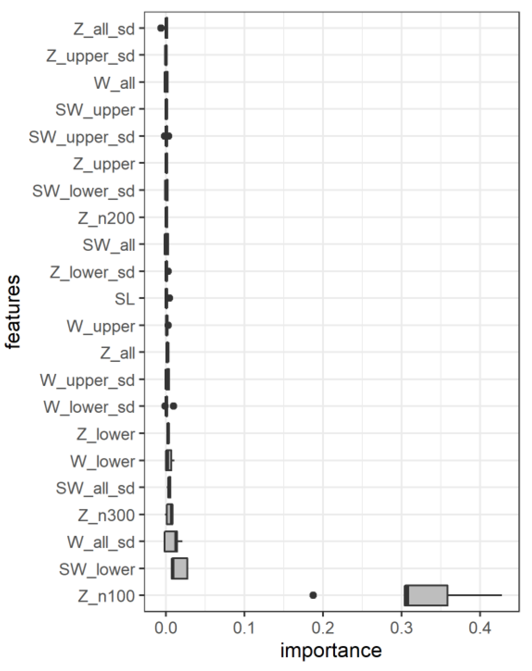
2.6. Model Interpretation

Complex machine learning models often lack interpretability. To gain some insights into such models and their main drivers, we apply interpretability methods of the research area interpretable machine learning (IML) [57]. In general, global and local IML methods can be distinguished. While global IML methods try to explain the general behavior of the model for the entire dataset, local methods try to find explanations for single predictions and thus for individual instances of the dataset.

A commonly used method to rank features according to their importance is the permutation feature importance (PFI) [58]. The PFI identifies the most important features for the performance of the model. To calculate the PFI of a feature x, we permute only the feature x to break the association between this feature and the target variable. Then, we predict with the ML model at hand on the modified dataset and calculate how much the performance (AUC) drops compared to the original dataset. This drop in performance then tells us how important feature x is for the model’s predictive performance.

To see how a specific feature affects the model’s prediction, effect plots such as partial dependence plots (PDPs) can be used. PDPs [50] show the average marginal prediction for a feature of interest. Individual conditional expectation (ICE) curves represent the marginal prediction on the observation level and hence give further insights into the models’ behavior [59].

A popular method to understand how different features of a dataset influence a single model’s prediction is Shapley values [60,61]. Shapley values are based on game theory. The main idea behind this method is to fairly distribute a payoff (here, a model’s prediction) among all players (features).

3. Results

3.1. Overall Model Performance

Evaluating the overall performance of each of the seven models revealed that the more complex models (xgboost, rf, and svm) performed on average better than simpler baseline models (

Table 4. Comparison of tuned ML models and baseline models where convective was chosen to be the positive class (1) and stratiform was chosen to be the negative class (0). The arithmetic mean (standard deviation) of the AUC, BAC, F1 score, recall and precision are compared. Best scores are the closest to 1 and are underlined and in bold.

	Model	AUC	BAC	F1	Recall	Precision
baseline	naïve Bayes	0.87 (0.11)	0.81 (0.10)	0.50 (0.08)	0.71 (0.20)	0.41 (0.10)
	log reg	0.95 (0.03)	0.77 (0.03)	0.63 (0.06)	0.56 (0.06)	0.73 (0.09)
	tree	0.94 (0.04)	0.80 (0.08)	0.66 (0.08)	0.63 (0.18)	0.76 (0.14)
tuned	knn	0.93 (0.02)	0.73 (0.05)	0.57 (0.07)	0.49 (0.10)	0.73 (0.10)
	svm	0.96 (0.02)	0.80 (0.07)	0.65 (0.09)	0.61 (0.14)	0.72 (0.06)
	rf	0.96 (0.02)	0.81 (0.06)	0.70 (0.08)	0.65 (0.12)	0.77 (0.09)
	xgboost	0.97 (0.01)	0.82 (0.04)	0.71 (0.05)	0.66 (0.09)	0.78 (0.07)

). This is evident particularly for xgboost and rf in terms of the high average and relatively small standard deviation of five outer fold validation performance values of AUC, BAC, F1, and precision. This justifies applying a complex ML model to this classification task. The naïve Bayes model scored the highest recall value. However, its precision was the worst (0.41). This indicates that 59% of the minutes which are classified as convective by the naïve Bayes model are false positives. In comparison, xgboost almost doubles the precision (0.78) without a drastic compromise of the recall.

3.2. Model Interpretation

xgboost performed best on the given dataset (Table 4). Therefore, we choose the xgboost model for further analysis. In particular, we are interested in what have been the most influential features to achieve this performance and how these features influence the model’s prediction. Furthermore, we analyze how well the model performs on unseen test events and identify the main drivers for these predictions.

First, we calculate the permutation feature importance (PFI) on the feature level [58] to identify the most important features for the performance of the model. According to PFI on the feature level (Figure 4), the by far most important feature is the Z value at the lowest measured height (Z_n100) followed by the average value of SW below the SL. Both these features indicate the conditions at the height near the disdrometer which is used for true labeling.

PFI can also be calculated for a group of features [62], given that grouping these features is meaningful. Grouping features by the measured parameter (Z, W, SW) and aggregation technique (arithmetic mean, standard deviation) revealed that Z values at the lower heights are the most important features for the model’s performance while mean SW measurements are the second most important group and the standard deviation value of W measurements are on rank three. Another grouping approach was based on the aggregation technique and the spatial position of the measurements (lower, upper, and whole column). Mean values below SL had the highest importance and were followed by the standard deviation of the values over the whole column (Figure A1). The remaining feature groups seem to be less important for the predictive performance of the model. The grouped feature importance scores also show that they do not necessarily add up the individual importance scores of the features. This effect is due to feature correlations and interactions [62]. Hence, individual importance scores do not fully reveal the influence of features on the target which is also shown in the next analysis on feature effects.

The PDP and ICE curves are shown for Z_n100 as the most important feature in Figure 5a. This feature distinguishes very well between the two rain classes based on its value. Low values of Z_n100 most of the time classify a minute as stratiform, while minutes with high values of Z_n100 are very likely predicted as convective. This is particularly true when Z_n100 is greater than 40 dBZ, a key value which has been used in the past for detecting convective rain [21]. The second most important feature SW_lower shows the opposite trend (Figure 5b): The lower the value, the more likely it is that the minute is classified as convective. The heterogeneous ICE curves in both plots are an indicator that interactions between the respective features and other features are present. These plots emphasize that more complex relationships (including feature interactions) have been modeled by the xgboost model, which might be a further indicator that the underlying relationships in the data are more complex. This is also in line with the shown outperformance of the xgboost model compared to simple baseline models such as logistic regression.

3.3. Model Results for Specific Events

Despite a global view of the model and data, local explanations for single events might be useful to understand why misclassifications occur. We will have a look at the left-out test set which are rain event numbers 186, 191, 196, and 204. While event 196 is almost completely a stratiform rain event (Figure 6), the events 186 and 191 are rather mixed (Figure A2 and Figure A3). We calculated Shapley values [60] for each minute, which show the contribution of each feature to the actual prediction compared to the average prediction (in the case of convective rain ~0.1). The individual Shapley values indicate clear clusters of convective and stratiform classes in terms of Z_n100 at events 186, 191, and 196 (Figure 7). Only 9 min were wrongly classified in these three events, and they mostly occur at the transitional phase between the two rain classes, either preceding or following a convective phase. Event 204, however, contained the most misclassification cases. Shapley values of Z_n100 show stratiform minutes with particularly high values within the convective range. Similarly, a number of convective minutes appear with a relatively low Shapley value of Z_n100 (Figure 7).

During event 204, xgboost agreed with Br09 on 83 min as convective rain and 275 min as stratiform rain. The discrepancies occurred in 20 cases of false negatives and 35 cases of false positives out of 396 min in total. This event had a high rain intensity exceeding 5 mm/h for more than 90 min. However, a melting layer is clearly identified throughout the whole event (Figure 8). A subjective classifier would classify all minutes within this event as stratiform, however, the rain intensity and the microstructure which are observed on the ground by the disdrometer imply convective rain.

4. Discussion

The application of machine learning models in meteorological studies, particularly in the remote sensing area, is gaining more focus. Such models could be used to partition areas into non-rain, convective, or stratiform based on satellite data [63,64], and ground-based radar data [65,66]. However, ML models need to be performed carefully as they do not necessarily outperform other statistical models [67]. Despite this accelerating interest in ML and its applications, only one study applied artificial neural network (ANN) models to this classification task using MRR data [37]. The method successfully detects high percentages of convective and stratiform rain. Despite the promising high performance of such deep learning models, they have disadvantages related to the design of the neural network structure, tuning, and interpretability. Therefore, we restricted our choice to the aforementioned three simple and four flexible ML models. One major difference in our study is the use of strictly two classes of rain and not assigning a third inconclusive class. The third, transitional class of rain can be assigned to minutes where −0.1 < i < 0.1 [39], or −0.3 < i < 0.3 [32]. In an attempt to avoid the influence of subjective choice of this threshold, only two classes of rain were chosen. This, besides the choice of classification features, and the different approaches to include the temporal variability, precludes a true performance comparison.

The steps of feature engineering include summarizing the MRR output in terms of means and standard deviations within regions above and below the separation level over periods of five minutes. Since the existence of a melting layer is “sufficient but not necessary” in stratiform rain [21], our suggestion to introduce the concept of a separation level is crucial; it brings in the common knowledge of differences between the regions above and below the melting layer in stratiform rain, without strictly classifying the rain based on the existence or non-existence of this layer. Stratiform rain may occur without a melting layer being observed. This may happen during the periods leading or tailing a convective period, and in case the melting layer forms above the range of elevations observed by the MRR. The averaging over periods of five minutes enables accounting for time dependencies without including them in the model itself. Creating three or more lagged values of three features and 30 elevations might then already be quite a huge matrix.

The interplay between different features might be an explanation for the good performance of tree-based models; xgboost achieved the highest performance indicators in this classification task, followed closely by rf. Similarly, the decision tree baseline model performed quite well, exceeding knn, and on par with svm. These tree-based predictive models are very well suited to capture lower- as well as higher-order interaction terms. This also explains the repeated success of random forest at precipitation classification tasks [64,68].

Many studies pointed out the importance of specific parameters to detect the melting layer, and classify rain. Radar reflectivity comes at the top of these parameters in most cases as an average over the whole column, as a maximum value, or as a bright band that indicates a melting layer (Table 1). Our results rank reflectivity at the lower heights as the most important feature for classification performance. This is consistent with previous classification methods which set a reflectivity value of 40 dBZ as a typical threshold for identifying convective rain [21]. Doppler velocity was also used widely to identify the melting layer and classify rain such as in [33,34]. However, our results indicate that Doppler velocity importance as a classifying feature is exceeded by a couple of features, namely the mean spectral width at the lower region, and the variability of Doppler velocity for the whole column. The relevance found of the SW is consistent with previous studies [29,69] where SW profiles of stratiform presented higher peaks than convective profiles, particularly of shallow convective cases when there were no hydrometeors above the melting level. Our results indicate that low SW_lower values are associated with higher probability of convection. This is likely because some of the convective cases detected are shallow convection cases as reported by Tokay et al. [69]. In their study, deep convective cases had SW as stratiform cases below the melting level but higher than shallow convective cases, particularly for low rainfall rates.

The existence of a melting layer is typically associated with a low rain rate [35,70,71,72]. However, event 204 is characterized by a high rain intensity and a clear melting layer. This event demonstrates a contradiction between an objective classifier and the BR09 method. It also witnessed the highest disagreement between BR09 and the tuned xgboost model. The contradiction highlights that an ML model would not be able to outperform the training method. Despite our approach and aim at an objective classification process, the existence of such stratiform events with a very high rain intensity calls for special measures to avoid misclassification. Additionally, different mixes of physical processes dominate precipitation at different locations globally and contribute to the variability of surface raindrop size distribution observations [1]. This raises the concern of achieving a robust rain type classification performance when labeling rain type based on ground observation of raindrop size distribution. Possible solutions may include a change in the labeling process of the training set. An ensemble of subjective and objective classifiers may be used or combining the objectively classified events with several events which are pre-labeled by an expert.

While disdrometers produce rain data as observed on the ground, Micro Rain Radars provide observations of the whole column above the point of interest. Precipitating hydrometeors observed by the MRR at different levels reach the disdrometer with a delay depending on the height, an effect that may be amplified by strong winds. This justifies the use of a wider temporal window and partially explains the discrepancies between classification methods that use MRR and disdrometers, especially at periods preceding or tailing a convective cell. The side wind also plays a role in pushing meteors that are within the MRR observation range away from the disdrometer observation area.

5. Conclusions

The separation level is defined as the elevation with the highest increase in Doppler velocity. Subsequently, MRR measurements of Z, W, and SW were summarized above and below the separation level into 22 features and used to classify rain type at Das, based on the method of BR09 and a collocated disdrometer. A comparison of the classification performance of four machine learning models and three baseline models identified tree-based machine learning models, particularly xgboost and rf, as the most appropriate for classifying rain type. While the highest importance was assigned to reflectivity close to the ground level and to the spectral width below the separation level, the high performance of tree-based methods emphasizes the role of interactions among the 22 features. Future research may experiment with different true labeling approaches and include different locations globally to account for the possible spatial variability in rain microstructure and the shortcomings of the point measurements of disdrometers.

References

1. Dolan, B.; Fuchs, B.; Rutledge, S.A.; Barnes, E.A.; Thompson, E.J. Primary Modes of Global Drop Size Distributions. J. Atmos. Sci. 2018, 75, 1453–1476. [Google Scholar] [CrossRef]
2. Sreekanth, T.S.; Varikoden, H.; Resmi, E.A.; Mohan Kumar, G. Classification and seasonal distribution of rain types based on surface and radar observations over a tropical coastal station. Atmos. Res. 2019, 218, 90–98. [Google Scholar] [CrossRef]
3. Wen, L.; Zhao, K.; Wang, M.; Zhang, G. Seasonal Variations of Observed Raindrop Size Distribution in East China. Adv. Atmos. Sci. 2019, 36, 346–362. [Google Scholar] [CrossRef]
4. Dai, A. Global Precipitation and Thunderstorm Frequencies. Part I: Seasonal and Interannual Variations. J. Clim. 2001, 14, 1092–1111. [Google Scholar] [CrossRef]
5. Chernokulsky, A.; Kozlov, F.; Zolina, O.; Bulygina, O.; Mokhov, I.I.; Semenov, V.A. Observed changes in convective and stratiform precipitation in Northern Eurasia over the last five decades. Environ. Res. Lett. 2019, 14, 45001. [Google Scholar] [CrossRef]
6. Ghada, W.; Buras, A.; Lüpke, M.; Schunk, C.; Menzel, A. Rain Microstructure Parameters Vary with Large-Scale Weather Conditions in Lausanne, Switzerland. Remote Sens. 2018, 10, 811. [Google Scholar] [CrossRef]
7. Arulraj, M.; Barros, A.P. Improving quantitative precipitation estimates in mountainous regions by modelling low-level seeder-feeder interactions constrained by Global Precipitation Measurement Dual-frequency Precipitation Radar measurements. Remote Sens. Environ. 2019, 231, 111213. [Google Scholar] [CrossRef]
8. Kühnlein, M.; Appelhans, T.; Thies, B.; Nauss, T. Improving the accuracy of rainfall rates from optical satellite sensors with machine learning—A random forests-based approach applied to MSG SEVIRI. Remote Sens. Environ. 2014, 141, 129–143. [Google Scholar] [CrossRef]
9. Steiner, M.; Houze, R.A. Sensitivity of the Estimated Monthly Convective Rain Fraction to the Choice of Z—R Relation. J. Appl. Meteor. 1997, 36, 452–462. [Google Scholar] [CrossRef]
10. Thompson, E.J.; Rutledge, S.A.; Dolan, B.; Thurai, M. Drop Size Distributions and Radar Observations of Convective and Stratiform Rain over the Equatorial Indian and West Pacific Oceans. J. Atmos. Sci. 2015, 72, 4091–4125. [Google Scholar] [CrossRef]
11. Berg, P.; Moseley, C.; Haerter, J.O. Strong increase in convective precipitation in response to higher temperatures. Nat. Geosci. 2013, 6, 181–185. [Google Scholar] [CrossRef]
12. Langer, I.; Reimer, E. Separation of convective and stratiform precipitation for a precipitation analysis of the local model of the German Weather Service. Adv. Geosci. 2007, 10, 159–165. [Google Scholar] [CrossRef]
13. Llasat, M.-C. An objective classification of rainfall events on the basis of their convective features: Application to rainfall intensity in the northeast of spain. Int. J. Climatol. 2001, 21, 1385–1400. [Google Scholar] [CrossRef]
14. Bringi, V.N.; Chandrasekar, V.; Hubbert, J.; Gorgucci, E.; Randeu, W.L.; Schoenhuber, M. Raindrop Size Distribution in Different Climatic Regimes from Disdrometer and Dual-Polarized Radar Analysis. J. Atmos. Sci. 2003, 60, 354–365. [Google Scholar] [CrossRef]
15. Testud, J.; Oury, S.; Amayenc, P. The concept of “normalized” distribution to describe raindrop spectra: A tool for hydrometeor remote sensing. Phys. Chem. Earth Part B Hydrol. Ocean. Atmos. 2000, 25, 897–902. [Google Scholar] [CrossRef]
16. Hachani, S.; Boudevillain, B.; Delrieu, G.; Bargaoui, Z. Drop Size Distribution Climatology in Cévennes-Vivarais Region, France. Atmosphere 2017, 8, 233. [Google Scholar] [CrossRef]
17. Ghada, W.; Bech, J.; Estrella, N.; Hamann, A.; Menzel, A. Weather Types Affect Rain Microstructure: Implications for Estimating Rain Rate. Remote Sens. 2020, 12, 3572. [Google Scholar] [CrossRef]
18. Tokay, A.; Short, D.A. Evidence from Tropical Raindrop Spectra of the Origin of Rain from Stratiform versus Convective Clouds. J. Appl. Meteor. 1996, 35, 355–371. [Google Scholar] [CrossRef]
19. Caracciolo, C.; Porcù, F.; Prodi, F. Precipitation classification at mid-latitudes in terms of drop size distribution parameters. Adv. Geosci. 2008, 16, 11–17. [Google Scholar] [CrossRef]
20. Bringi, V.N.; Williams, C.R.; Thurai, M.; May, P.T. Using Dual-Polarized Radar and Dual-Frequency Profiler for DSD Characterization: A Case Study from Darwin, Australia. J. Atmos. Oceanic Technol. 2009, 26, 2107–2122. [Google Scholar] [CrossRef]
21. Steiner, M.; Houze, R.A.; Yuter, S.E. Climatological Characterization of Three-Dimensional Storm Structure from Operational Radar and Rain Gauge Data. J. Appl. Meteor. 1995, 34, 1978–2007. [Google Scholar] [CrossRef]
22. Churchill, D.D.; Houze, R.A. Development and Structure of Winter Monsoon Cloud Clusters On 10 December 1978. J. Atmos. Sci. 1984, 41, 933–960. [Google Scholar] [CrossRef]
23. Berendes, T.A.; Mecikalski, J.R.; MacKenzie, W.M.; Bedka, K.M.; Nair, U.S. Convective cloud identification and classification in daytime satellite imagery using standard deviation limited adaptive clustering. J. Geophys. Res. 2008, 113, D20207. [Google Scholar] [CrossRef]
24. Anagnostou, E.N.; Kummerow, C. Stratiform and Convective Classification of Rainfall Using SSM/I 85-GHz Brightness Temperature Observations. J. Atmos. Oceanic Technol. 1997, 14, 570–575. [Google Scholar] [CrossRef]
25. Adler, R.F.; Negri, A.J. A Satellite Infrared Technique to Estimate Tropical Convective and Stratiform Rainfall. J. Appl. Meteor. 1988, 27, 30–51. [Google Scholar] [CrossRef]
26. Fabry, F.; Zawadzki, I. Long-Term Radar Observations of the Melting Layer of Precipitation and Their Interpretation. J. Atmos. Sci. 1995, 52, 838–851. [Google Scholar] [CrossRef]
27. Garcia-Benadi, A.; Bech, J.; Gonzalez, S.; Udina, M.; Codina, B.; Georgis, J.-F. Precipitation Type Classification of Micro Rain Radar Data Using an Improved Doppler Spectral Processing Methodology. Remote Sens. 2020, 12, 4113. [Google Scholar] [CrossRef]
28. Garcia-Benadí, A.; Bech, J.; Gonzalez, S.; Udina, M.; Codina, B. A New Methodology to Characterise the Radar Bright Band Using Doppler Spectral Moments from Vertically Pointing Radar Observations. Remote Sens. 2021, 13, 4323. [Google Scholar] [CrossRef]
29. Williams, C.R.; Ecklund, W.L.; Gage, K.S. Classification of Precipitating Clouds in the Tropics Using 915-MHz Wind Profilers. J. Atmos. Oceanic Technol. 1995, 12, 996–1012. [Google Scholar] [CrossRef]
30. White, A.B.; Neiman, P.J.; Ralph, F.M.; Kingsmill, D.E.; Persson, P.O.G. Coastal Orographic Rainfall Processes Observed by Radar during the California Land-Falling Jets Experiment. J. Hydrometeor. 2003, 4, 264–282. [Google Scholar] [CrossRef]
31. Cha, J.-W.; Chang, K.-H.; Yum, S.S.; Choi, Y.-J. Comparison of the bright band characteristics measured by Micro Rain Radar (MRR) at a mountain and a coastal site in South Korea. Adv. Atmos. Sci. 2009, 26, 211–221. [Google Scholar] [CrossRef]
32. Thurai, M.; Gatlin, P.N.; Bringi, V.N. Separating stratiform and convective rain types based on the drop size distribution characteristics using 2D video disdrometer data. Atmos. Res. 2016, 169, 416–423. [Google Scholar] [CrossRef]
33. Massmann, A.K.; Minder, J.R.; Garreaud, R.D.; Kingsmill, D.E.; Valenzuela, R.A.; Montecinos, A.; Fults, S.L.; Snider, J.R. The Chilean Coastal Orographic Precipitation Experiment: Observing the Influence of Microphysical Rain Regimes on Coastal Orographic Precipitation. J. Hydrometeor. 2017, 18, 2723–2743. [Google Scholar] [CrossRef]
34. Gil-de-Vergara, N.; Riera, J.M.; Pérez-Peña, S.; Garcia-Rubia, J.; Benarroch, A. Classification of rainfall events and evaluation of drop size distributions using a k-band doppler radar. In Proceedings of the 12th European Conference on Antennas and Propagation (EuCAP 2018), 9–13 April 2018; Institution of Engineering and Technology: London, UK, 2018; p. 829, ISBN 978-1-78561-816-1. [Google Scholar]
35. Seidel, J.; Trachte, K.; Orellana-Alvear, J.; Figueroa, R.; Célleri, R.; Bendix, J.; Fernandez, C.; Huggel, C. Precipitation Characteristics at Two Locations in the Tropical Andes by Means of Vertically Pointing Micro-Rain Radar Observations. Remote Sens. 2019, 11, 2985. [Google Scholar] [CrossRef]
36. Rajasekharan Nair, H. Discernment of near-oceanic precipitating clouds into convective or stratiform based on Z–R model over an Asian monsoon tropical site. Meteorol. Atmos. Phys. 2020, 132, 377–390. [Google Scholar] [CrossRef]
37. Foth, A.; Zimmer, J.; Lauermann, F.; Kalesse-Los, H. Evaluation of micro rain radar-based precipitation classification algorithms to discriminate between stratiform and convective precipitation. Atmos. Meas. Tech. 2021, 14, 4565–4574. [Google Scholar] [CrossRef]
38. Thurai, M.; Bringi, V.; Wolff, D.; Marks, D.; Pabla, C. Testing the Drop-Size Distribution-Based Separation of Stratiform and Convective Rain Using Radar and Disdrometer Data from a Mid-Latitude Coastal Region. Atmosphere 2021, 12, 392. [Google Scholar] [CrossRef]
39. Thurai, M.; Bringi, V.N.; May, P.T. CPOL Radar-Derived Drop Size Distribution Statistics of Stratiform and Convective Rain for Two Regimes in Darwin, Australia. J. Atmos. Oceanic Technol. 2010, 27, 932–942. [Google Scholar] [CrossRef]
40. Udina, M.; Bech, J.; Gonzalez, S.; Soler, M.R.; Paci, A.; Miró, J.R.; Trapero, L.; Donier, J.M.; Douffet, T.; Codina, B.; et al. Multi-sensor observations of an elevated rotor during a mountain wave event in the Eastern Pyrenees. Atmos. Res. 2020, 234, 104698. [Google Scholar] [CrossRef]
41. Cerro, C.; Codina, B.; Bech, J.; Lorente, J. Modeling Raindrop Size Distribution and Z (R) Relations in the Western Mediterranean Area. J. Appl. Meteor. 1997, 36, 1470–1479. [Google Scholar] [CrossRef]
42. Cerro, C.; Bech, J.; Codina, B.; Lorente, J. Modeling Rain Erosivity Using Disdrometric Techniques. Soil Sci. Soc. Am. J. 1998, 62, 731–735. [Google Scholar] [CrossRef]
43. R Core Team. R: A Language and Environment for Statistical Computing; R Foundation for Statistical Computing: Vienna, Austria, 2021; Available online: https://www.R-project.org/ (accessed on 12 July 2022).
44. Löffler-Mang, M.; Joss, J. An Optical Disdrometer for Measuring Size and Velocity of Hydrometeors. J. Atmos. Oceanic Technol. 2000, 17, 130–139. [Google Scholar] [CrossRef]
45. Friedrich, K.; Kalina, E.A.; Masters, F.J.; Lopez, C.R. Drop-Size Distributions in Thunderstorms Measured by Optical Disdrometers during VORTEX2. Mon. Wea. Rev. 2013, 141, 1182–1203. [Google Scholar] [CrossRef]
46. Löffler-Mang, M.; Kunz, M.; Schmid, W. On the Performance of a Low-Cost K-Band Doppler Radar for Quantitative Rain Measurements. J. Atmos. Oceanic Technol. 1999, 16, 379–387. [Google Scholar] [CrossRef]
47. Gonzalez, S.; Bech, J.; Udina, M.; Codina, B.; Paci, A.; Trapero, L. Decoupling between Precipitation Processes and Mountain Wave Induced Circulations Observed with a Vertically Pointing K-Band Doppler Radar. Remote Sens. 2019, 11, 1034. [Google Scholar] [CrossRef]
48. Cover, T.; Hart, P. Nearest neighbor pattern classification. IEEE Trans. Inform. Theory 1967, 13, 21–27. [Google Scholar] [CrossRef]
49. Breiman, L. Random Forests. Mach. Learn. 2001, 45, 5–32. [Google Scholar] [CrossRef]
50. Friedman, J.H. Greedy function approximation: A gradient boosting machine. Ann. Statist. 2001, 29, 1189–1232. [Google Scholar] [CrossRef]
51. Chen, T.; He, T.; Benesty, M.; Khotilovich, V.; Tang, Y.; Cho, H.; Chen, K. Xgboost: Extreme gradient boosting. R Package Version 0.4-2. 2015, Volume 1, pp. 1–4. Available online: https://cran.microsoft.com/snapshot/2017-12-11/web/packages/xgboost/vignettes/xgboost.pdf (accessed on 12 July 2022).
52. Cervantes, J.; Garcia-Lamont, F.; Rodríguez-Mazahua, L.; Lopez, A. A comprehensive survey on support vector machine classification: Applications, challenges and trends. Neurocomputing 2020, 408, 189–215. [Google Scholar] [CrossRef]
53. Bischl, B.; Binder, M.; Lang, M.; Pielok, T.; Richter, J.; Coors, S.; Thomas, J.; Ullmann, T.; Becker, M.; Boulesteix, A.-L.; et al. Hyperparameter Optimization: Foundations, Algorithms, Best Practices and Open Challenges. 2021. Available online: https://arxiv.org/pdf/2107.05847 (accessed on 12 July 2022).
54. Varma, S.; Simon, R. Bias in error estimation when using cross-validation for model selection. BMC Bioinform. 2006, 7, 91. [Google Scholar] [CrossRef] [Green Version]
55. López-Ibáñez, M.; Dubois-Lacoste, J.; Pérez Cáceres, L.; Birattari, M.; Stützle, T. The irace package: Iterated racing for automatic algorithm configuration. Oper. Res. Perspect. 2016, 3, 43–58. [Google Scholar] [CrossRef]
56. Becker, M.; Binder, M.; Bischl, B.; Foss, N.; Kotthoff, L.; Lan, M.; Pfisterer, F.; Reich, N.G.; Richter, J.; Schratz, P.; et al. mlr3book. Available online: https://mlr3book.mlr-org.com (accessed on 1 September 2022).
57. Molnar, C. Interpretable Machine Learning: A Guide for Making Black Box Models Explainable, 2nd ed.; Lulu: Morisville, NC, USA, 2022; Available online: https://christophm.github.io/interpretable-ml-book (accessed on 12 July 2022).
58. Fisher, A.; Rudin, C.; Dominici, F. All Models are Wrong, but Many are Useful: Learning a Variable’s Importance by Studying an Entire Class of Prediction Models Simultaneously. J. Mach. Learn. Res. 2019, 20, 1–81. [Google Scholar]
59. Goldstein, A.; Kapelner, A.; Bleich, J.; Pitkin, E. Peeking Inside the Black Box: Visualizing Statistical Learning with Plots of Individual Conditional Expectation. J. Comput. Graph. Stat. 2015, 24, 44–65. [Google Scholar] [CrossRef]
60. Shapley, L.S. 17. A Value for n-Person Games. In Contributions to the Theory of Games (AM-28), Volume II; Kuhn, H.W., Tucker, A.W., Eds.; Princeton University Press: Princeton, NJ, USA, 1953; pp. 307–318. ISBN 9781400881970. [Google Scholar]
61. Lundberg, S.M.; Lee, S.-I. A unified approach to interpreting model predictions. In Proceedings of the 31st International Conference on Neural Information Processing Systems; 2017; pp. 4768–4777. Available online: https://arxiv.org/pdf/1705.07874 (accessed on 1 September 2022).
62. Au, Q.; Herbinger, J.; Stachl, C.; Bischl, B.; Casalicchio, G. Grouped feature importance and combined features effect plot. Data Min. Knowl. Disc. 2022, 36, 1401–1450. [Google Scholar] [CrossRef]
63. Upadhyaya, S.A.; Kirstetter, P.-E.; Kuligowski, R.J.; Searls, M. Classifying precipitation from GEO satellite observations: Diagnostic model. Q. J. R. Meteorol. Soc. 2021, 147, 3318–3334. [Google Scholar] [CrossRef]
64. Ouallouche, F.; Lazri, M.; Ameur, S. Improvement of rainfall estimation from MSG data using Random Forests classification and regression. Atmos. Res. 2018, 211, 62–72. [Google Scholar] [CrossRef]
65. Song, J.J.; Innerst, M.; Shin, K.; Ye, B.-Y.; Kim, M.; Yeom, D.; Lee, G. Estimation of Precipitation Area Using S-Band Dual-Polarization Radar Measurements. Remote Sens. 2021, 13, 2039. [Google Scholar] [CrossRef]
66. Yang, Z.; Liu, P.; Yang, Y. Convective/Stratiform Precipitation Classification Using Ground-Based Doppler Radar Data Based on the K-Nearest Neighbor Algorithm. Remote Sens. 2019, 11, 2277. [Google Scholar] [CrossRef]
67. Wang, J.; Wong, R.K.W.; Jun, M.; Schumacher, C.; Saravanan, R.; Sun, C. Statistical and machine learning methods applied to the prediction of different tropical rainfall types. Environ. Res. Commun. 2021, 3, 111001. [Google Scholar] [CrossRef] [PubMed]
68. Seo, B.-C. A Data-Driven Approach for Winter Precipitation Classification Using Weather Radar and NWP Data. Atmosphere 2020, 11, 701. [Google Scholar] [CrossRef]
69. Tokay, A.; Short, D.A.; Williams, C.R.; Ecklund, W.L.; Gage, K.S. Tropical Rainfall Associated with Convective and Stratiform Clouds: Intercomparison of Disdrometer and Profiler Measurements. J. Appl. Meteor. 1999, 38, 302–320. [Google Scholar] [CrossRef]
70. Das, S.; Shukla, A.K.; Maitra, A. Investigation of vertical profile of rain microstructure at Ahmedabad in Indian tropical region. Adv. Space Res. 2010, 45, 1235–1243. [Google Scholar] [CrossRef]
71. Das, S.; Maitra, A. Vertical profile of rain: Ka band radar observations at tropical locations. J. Hydrol. 2016, 534, 31–41. [Google Scholar] [CrossRef]
72. Urgilés, G.; Célleri, R.; Trachte, K.; Bendix, J.; Orellana-Alvear, J. Clustering of Rainfall Types Using Micro Rain Radar and Laser Disdrometer Observations in the Tropical Andes. Remote Sens. 2021, 13, 991. [Google Scholar] [CrossRef]
Figure 1. Measurement location at the Das aerodrome in northeast Spain. The aerodrome location (1100 m a.s.l.) is marked with a red circle in the right panel.
Remotesensing 14 04563 g001
Figure 2. Separation level in stratiform and convective events. The Doppler velocity W is represented for a stratiform event (a) and a convective event (b). Identifying the separation level for a five-minute window (c) requires identifying for each minute the height in which the change in SW is the maximum (blue stars), then finding the mean of the five heights (the height of the layer in yellow).
Remotesensing 14 04563 g002
Figure 3. Representation of the nested cross-validation approach for tuning and measuring the performance of the chosen ML models based on [56]. Within each of the 5 outer folds, a holdout strategy to tune the hyperparameters is carried out. The best found hyperparameters are then evaluated on the test set of the outer fold.
Remotesensing 14 04563 g003
Figure 4. The importance of individual features ordered by the mean value of permutation feature importance (PFI) for all 5 folds of the cross-validation. It shows the negative difference in AUC performance values between the original and modified dataset to receive positive PFI values. The left (right) hinges represent the first (third) quartiles, while the whiskers extend from the hinges to the smallest (largest) value no further than 1.5 times the interquartile range from the hinge, any value out of this range is considered as an outlier and is represented with a black dot.
Remotesensing 14 04563 g004
Figure 5. PDPs (yellow) and ICE curves (black) for the features (a) Z_n100 and (b) SW_lower for a tuned xgboost model on the entire training dataset.
Remotesensing 14 04563 g005
Figure 6. MRR and disdrometer data for event 196. The upper three panels represent the MRR measured values of reflectivity Z (dBZ), Doppler velocity W (m/sec), and spectral width SW (m/sec) respectively. The last panel represents rain intensity R (mm/h) as measured by the disdrometer.
Remotesensing 14 04563 g006
Figure 7. Shapley values of the most important two features for individual minutes across four events.
Remotesensing 14 04563 g007
Figure 8. MRR and disdrometer data for event 204. The upper three panels represent the MRR measured values of reflectivity Z (dBZ), Doppler velocity W (m/sec), and spectral width SW (m/sec) respectively. The last panel represents rain intensity R (mm/h) as measured by the disdrometer.
Remotesensing 14 04563 g008