
An Automatic Drift-Measurement-Data-Processing Method with Digital Ionosondes
by
 , ,
, ,
Xiaoya Ma
1,2,3 ,
,
Zhaoqian Gong
1,2,
Feng Zhang
1,2,*,
Shun Wang
1,2,
Xiaojun Liu
1,2 and
Guangyou Fang
1,2 1
Aerospace Information Research Institute, Chinese Academy of Sciences, Beijing 100190, China
2
Key Laboratory of Electromagnetic Radiation and Sensing Technology, Chinese Academy of Sciences, Beijing 100190, China
3
School of Electronic, Electrical and Communication Engineering, University of Chinese Academy of Sciences, Beijing 100049, China
*
Author to whom correspondence should be addressed.
Remote Sens. 2022, 14(19), 4710; https://0-doi-org.brum.beds.ac.uk/10.3390/rs14194710
Submission received: 25 July 2022
/
Revised: 10 September 2022
/
Accepted: 13 September 2022
/
Published: 21 September 2022
(This article belongs to the Topic High-Resolution Earth Observation Systems, Technologies, and Applications)
Abstract
:Drift detection is one of the important detection modes in a digital ionosonde system. In this paper, a new data processing method is presented for boosting the automatic and high-quality drift measurement, which is helpful for long-term ionospheric observation, and has been successfully applied to the Chinese Academy of Sciences, Digital Ionosonde (CAS-DIS). Based on Doppler interferometry principle, this method can be successively divided into four constraint steps: extracting the stable echo data; restricting the ionospheric detection region; extracting the reliable reflection cluster, including Doppler filtering and coarse clustering analysis; and calculating the drift velocity. Ordinary wave (O-wave) data extraction, complementary code pulse compression and other data preprocessing techniques are used to improve the signal-to-noise ratio (SNR) of echo data. For the purpose of eliminating multiple echoes, the ionospheric region is determined by combining the optimal height range and detection frequencies obtained from the ionogram. Successively, Doppler filtering and coarse clustering analysis extract reliable reflection clusters. Finally, the weighting factor is brought in, and then weighted least-squares (WLS) is used to fit the drift velocity. The entire data processing process can be implemented automatically without constantly changing parameter settings due to changes in external conditions. This is the first time coarse clustering analysis has been used to extract the paracentral reflection cluster to eliminate scattered reflection points and outer reflection clusters, which further reduces the impacts of external conditions on parameter settings and improves the ability of automatic drift measurement. Compared with the previous method possessed by Digisonde Protable Sounder 4D (DPS4D), the new method can achieve comparable drift detection precision and results even with fewer reflection points. In 2021–2022, several experiments on F region drift detection were carried out in Hainan, China. Results indicate that drift velocities fitted by the new method have diurnal variation and change more gently; the trends of drift velocities fitted by the new method and the previous method are semblable; and this new method can be widely applied to digital ionosondes.
1. Introduction
Ionospheric information is vital to human activities. Reliable long-distance shortwave communication depends heavily on ionospheric conditions [1]. This is because shortwave signals mainly bounce off the ionosphere before reaching the receiving equipment [2]. Ionospheric plasma drift is an important study direction derived from ionospheric variations. Typically, changes in the ionospheric plasma drift which trigger ionospheric scintillation have effects on global positioning systems [3]. Appropriately, digital ionosonde is a conventional terrestrial platform used to study the ionosphere, and its drift detection mode can measure the plasma drift velocity [4,5,6,7,8]. The drift velocity mentioned in this paper refers to the plasma drift velocity.
The early drift measurement methods estimated the drift velocity by using similar fading or correlation analyses which compared the amplitude fluctuations of the echoes received by the antenna array elements [9,10]. Then, Reinisch et al. initially presented Doppler interferometry to study drift velocity in 1998 [11]. The VFIT, which is essentially a deformation of Doppler interferometry, scales the phase measurements into a radial velocity [12]. Prominently, Doppler interferometry has the advantages of improving precision and simplifying calculations. It has also been applied to the American Digisonde family of ionospheric sounders [13], Canadian Advanced Digital Ionosonde (CADI) [14], Dynasonde [12] and so on. Compared with incoherent scatter radar observations, the reliability of ionosonde drift measurements at high, middle and low latitudes has been verified [15,16,17]. Comparison of the drift measurements by Dynasonde and EISCAT is consistent in the polar region [18]. A fair consistency about F-region drift measurements between ionosonde and incoherent scatter radar at magnetic equator has been reported [19].
However, using the raw echo data directly for drift measurements can reduce the accuracy of results. That is to say, clutter and multiple echoes mixed into the echoes can blur the ionospheric electron density profile. Some researchers used pulse compression, digital filtering, frequency domain correlation superposition, interference elimination algorithms, another WLS and other techniques to eliminate or suppress interference, so as to select reliable reflection points [4,20,21,22,23]. The above shows that a reliable data processing method is conducive to improving the accuracy of drift measurements, but the serious problem that data processing results are extremely sensitive to external conditions still exists. Considering that unmanned ionosonde stations demand real-time and long-term ionospheric monitoring, while guaranteeing accuracy, automating drift measurement is also essential.
Automatic drift measurement here does not mean that the program runs automatically, but rather that the parameter settings that have been set are little affected by changes in external conditions. In other words, when the external conditions change significantly, the previous methods must have their parameter settings modified in time to ensure the quality of the measurement. The method that DPS4D employs can be used as a typical example. The “ARTIST” function of this method enables autonomous selection of the detection frequencies, but not of the ionospheric region to be measured; this method has limited rejection of strong interference at high Doppler frequencies during Doppler filtering. The new method is an optimization of the previous method.
The proposed drift-measurement-data-processing method affects automatic drift measurements and enhances the quality of drift detection by successively implementing four steps: extracting the stable echo data, restricting the ionospheric detection region, extracting the reliable reflection cluster and calculating the drift velocity. Thus, parameter settings are not constantly changed as external conditions change. It is worth mentioning that clustering analysis is used for facilitating automatic drift measurement for the first time. The drift measurement results obtained by this constrained method agree well with those obtained by the method DPS4D uses, even with fewer reflection points. Experimental results show that the CAS-DIS employing this method can automatically control the drift measurement process and then get quality measurement results. This constrained data processing method is also applicable to other modern digital ionosondes.
Compared with existing drift-measurement-data-processing methods, the main innovations of this paper are as follows:
- The method realizes automatic and high-quality drift measurement and is dedicated to ionospheric drift detection, which can provide real-time and long-term ionospheric plasma drift state information.
- The method can be widely applied to digital ionosondes.
- The ionospheric detection region is constrained by detection frequencies and virtual heights provided by the ionogram, which effectively filters out the echoes from other regions.
- After Doppler filtering and coarse clustering analysis, the reliability of reflection points is enhanced, which could reduce the impacts of external conditions on parameter settings and further ensure the accuracy of the drift velocity.
2. Principle of the Drift Measurement
For the sake of drift detection, ionosonde primarily needs to vertically transmit pulse-modulated high-frequency radio waves from the ground. The radio waves are reflected when its frequencies equal that of the plasma, and they will be received by the antenna array later. As the actual ionospheric stratification is not smooth horizontal stratification, vertical and oblique echoes are received, which provides conditions for using the Doppler interferometry to calculate drift velocities.
The information of one echo data includes amplitudes, phases, virtual heights, echo directions and Doppler frequency shifts. The premise for Doppler interferometry is that all the plasma in the designated ionospheric region moves uniformly in a short time. Array-receiving interferometry can determine the directions of echo. Doppler frequency shifts can determine the drift radial velocities. Consequently, the drift velocity can be obtained by the correspondence between radial velocities and echo directions.
In terms of determining the echo direction, the dimensions of the receiving antenna are much smaller than the distance between the receiving antenna and the ionospheric detected region; hence, the echo can be regarded as the plane wave. When the i-th echo reaches the a-th receiving antenna, its phase is:
where is the wave vector of the i-th echo and is the vector from the first antenna to the a-th receiving antenna. Therefore, the phase difference of the i-th echo between the a-th receiving antenna and the b-th receiving antenna is:
According to Equation (2), can be determined. Then, the unit vector can be obtained from , where f is the drift detection frequency and c is the speed of light. Finally, the echo direction (azimuth angle and zenith angle ) from the i-th reflection point is calculated on the basis of .
In the process of determining the drift radial velocity, due to the relative motion between plasma and ionosonde, the echo certainly relates the Doppler frequency shift. The phase difference between the i-th echo and its transmitted signal is:
Double distance can be represented by
where is the time difference and is three-dimensional drift velocity. Accordingly, the Doppler frequency shift is further derived to
After simultaneous equations, the three-dimensional drift velocity in the geomagnetic coordinate system is
where , and are the drift velocity components. is the north–south drift velocity, which is positive when northward drift happens; is the east–west drift velocity, which is positive when eastward drift happens; is vertical drift velocity, which is positive when downward drift happens; zenith angle is 0° in the vertical downward drift direction and is positive away from this direction; azimuth angle is 0° in due north drift direction and is positive when it turns counterclockwise.
Equation (6) intuitively shows that the extraction quality of reflection points and the regression quality of drift velocities can directly affect the quality of the drift detection. The drift-measurement-data-processing method aims at obtaining the echo information of the first reflection points in the designated ionospheric region and obtaining a reliable drift velocity.
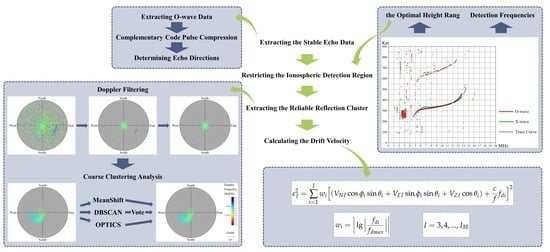
3. Method of the Drift Measurement Data Processing
This drift-measurement-data-processing method can be divided into four steps: extracting the stable echo data, restricting the ionospheric detection region, extracting the reliable reflection cluster and calculating the drift velocity.
3.1. Extracting the Stable Echo Data
When extracting the stable echo data, we firstly extract the high-resolution echo data with specified polarization, and then obtain the echo direction information. Extracting O-wave data, complementary code pulse compression and determining echo directions are the main parts of this step.
3.1.1. Extracting O-Wave Data
Considering the effect of the geomagnetic field, a radio wave splits into two characteristic waves with different refractive indexes and polarization states during the ionospheric propagation. One is the O-wave corresponding to a left-handed elliptic polarization wave, and the other is an unusual wave (X-wave) corresponding to a right-handed elliptic polarization wave. When the wave vector is parallel to the geomagnetic field, the O-wave is a left-handed circularly polarized wave and the X-wave is a right-handed circularly polarized wave; when the wave vector is perpendicular to the geomagnetic field, the O-wave is a linearly polarized north–south wave whose refraction index is unaffected by the geomagnetic field, and the X-wave is a linearly polarized east–west wave. Considering that the refraction index of an O-wave is relatively stable and the horizontal component of geomagnetic field is larger as it gets closer to the low latitudes, it is a more excellent choice to extract O-wave data for drift measurement.
A method for separating O-wave and X-wave data in the CAS-DIS system is realized by digitally synthesizing circularly polarized waves on the receiving circuit [24]. O-wave data are extracted by
where and , respectively, represent the real and virtual data of the east–west receiving antenna; and , respectively, represent the real and virtual data of the north–south receiving antenna. The echo data mentioned in the following all refer to O-wave data.
3.1.2. Complementary Code Pulse Compression
The CAS-DIS system uses complementary codes to phase modulate the carrier signal at the transmitter, and performs complementary code pulse compression on the baseband signal at the receiver for improving the SNR of echo data. The selected set of 16-bit complementary codes contains an A-code and a B-code. In order to reduce the calculation load, pulse compression could be implemented in the frequency domain. Above all, Fast Fourier Transform (FFT) is separately performed on the A-code and echo data modulated by the A-code; then, the two results above are multiplied, and the result is Inverse Fast Fourier Transformed (IFFT). Analogously, FFT is performed on the B-code and echo data modulated by the B-code; then, the two results above are multiplied, and IFFT is performed on the outcome. Lastly, the above two compression pulses are added to realize complementary code pulse compression processing. Figure 1 shows the autocorrelation processing results of complementary codes and the sum result of two autocorrelation functions, which reveals that the autocorrelation functions of A-code and B-code are opposite at the pseudo-correlation peak. By superposition of two compression pulses, the correlation peak rises to double with the same phase, and the pseudo-correlation peaks are canceled. The SNR is naturally enhanced.
After that, echo data passes through the median filter to reduce echo fluctuation and suppress noise. Additionally, the optimal window size of the median filter is 3–5 continuous echo data lengths.
3.1.3. Determining Echo Directions
The principle for determining echo directions has been interpreted in Section 2. Equation (2) indicates that at least three array elements are needed to solve . CAS-DIS adopts the triangular array of four array elements to receive echo data. Additionally, its is fitted by least-squares (LS):
where M is the number of elements. Then, the echo directions of all reflection points can be obtained.
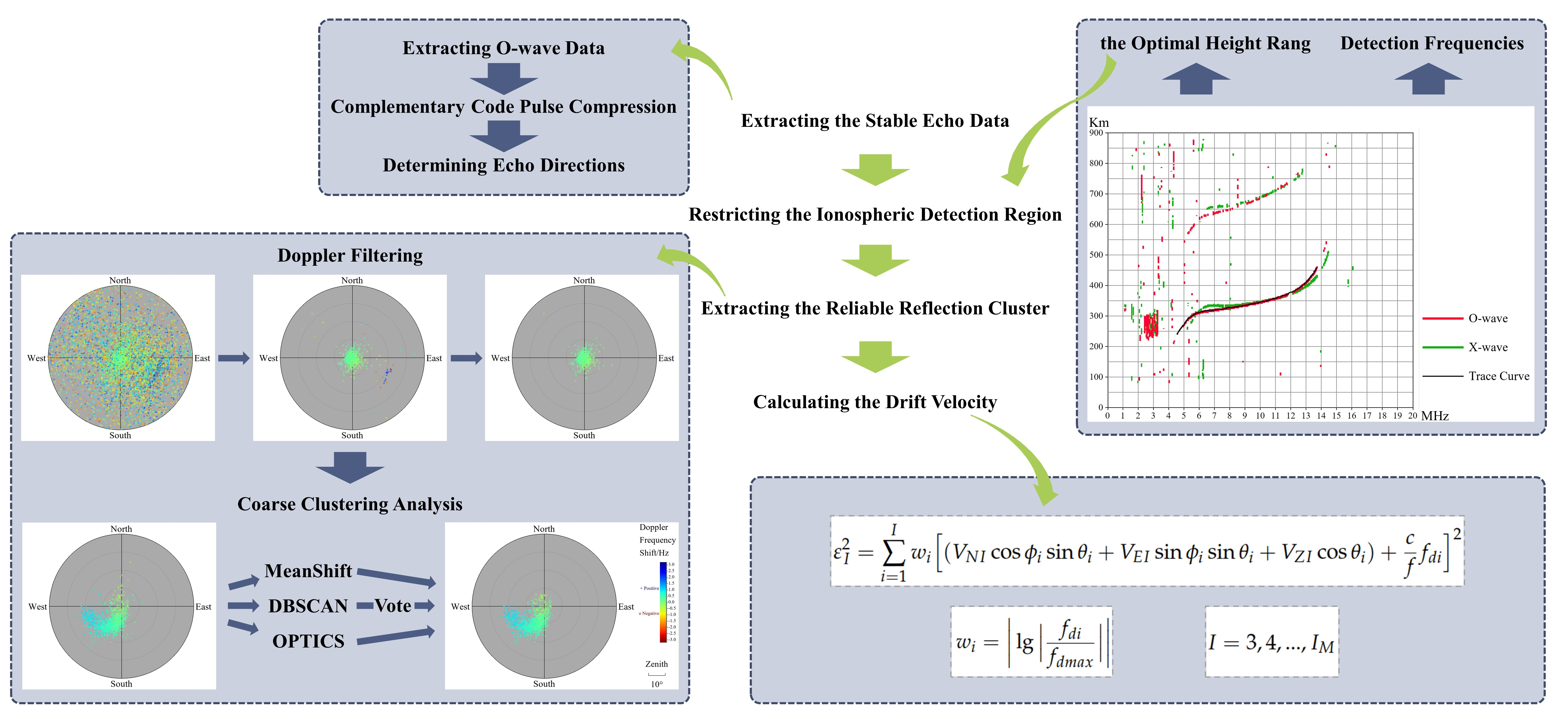
The skymap on the left of Figure 2 plots the distribution of reflection points. Additionally, the distance between the reflection point and the center of the skymap is proportional to the zenith angle.
3.2. Restricting the Ionospheric Detection Region
Since drift measurement is to measure the drift characteristics of the specified ionospheric region, it is incredibly necessary to distinguish the echoes from different ionospheric regions and eliminate the secondary echoes, multiple echoes and other clutter interference as far as it is possible.
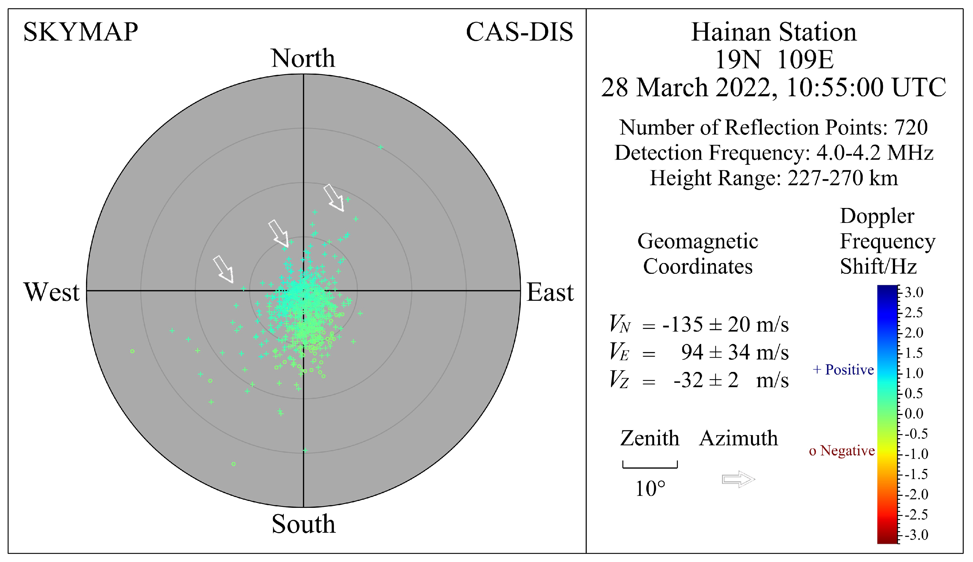
The ionogram (Figure 3), which charts the relationship curve between the detection frequency and the virtual height, shows that the strongest echo may be in E region or F region; may be a primary, secondary or multiple reflection echo; or may just be a false strongest echo. For this reason, selecting the detection frequency and restricting the height range are warranted. Height and height range in this article refer to virtual height and virtual height range. What should be noted is that the ionogram is the result of vertical detection, and its broadband characteristics are not appropriate for drift detection. This is because the drift measurement needs to meet the needs of large pulse accumulation times and real-time detection, resulting in a limited number of detection frequency points. Due to the small change of the ionosphere in the short term (about less than 5 min), CAS-DIS has the vertical detection and drift detection work alternately, and vertical detection is always about 3 min ahead of drift detection. In this way, the automatic calibration results of the ionogram, which are used for restricting the ionospheric detection region, can provide reliable parameters of detection frequencies and detection heights for drift measurement. The actual detection frequency is determined according to transmitted detection frequency parameters, and the actual detection height range is slightly wider than the range defined by transmitted detection height parameters.
During drift measurement, the height corresponding to the strongest echo in the detection height range is selected as the height of the primary reflection echo. The strongest echo is selected by the accumulation of multiple coherent pulses and the addition of data from four receiving channels at the same detection frequency. Given that the raw echo data are equal-spacing sampled and the ionosphere fluctuates during the detection, a narrow height range including the height of the primary reflection echo is selected as the optimal height range for drift measurement.
Figure 3 is the relevant case for detection frequency selection and optimal height range restriction. Figure 3a shows an invalid drift measurement without selecting reasonable detection frequencies; Figure 3b shows an invalid drift measurement with reasonable detection frequencies but no reasonable optimal height range. Its false optimal height range is 457–662 km, and thus the skymap reflects the mixed distribution of primary and secondary reflection points; Figure 3c describes the drift measurement with the reasonable detection frequencies and the reasonable optimal height range. Its optimal height range is 325–342 km, and thus the skymap reflects the distribution of primary reflection points; Figure 3d is an ionogram comprising the black trace curve of automatic calibration obtained 3 min before drift measurement (Figure 3a), and the wrong calibration result leads wrong parameters being transmitted to drift detection; Figure 3e is an ionogram whose detection and calibration results are obtained 3 min before drift measurement (Figure 3b,c). Several teams worldwide have been involved in the ionogram automatic calibration process for a long time [25,26,27,28].
3.3. Extracting the Reliable Reflection Cluster
On the premise of having extracted reliable echo data, Doppler filtering and coarse clustering analysis provide benign conditions for further implementation of automatic and stable drift measurement. Plainly, the reflection point information after multiple constraints (filtering) is the cornerstone of calculating the drift velocity.
3.3.1. Doppler Filtering
The higher the Doppler frequency resolution is, the better Doppler filtering performs. CAS-DIS can obtain high-Doppler-frequency resolution by adopting large pulse accumulation, which refers to the large number of single frequency pulse signals. When the data sampling rate is set to 20 Hz and pulse accumulation is set to 500 times, the Doppler frequency resolution can reach 0.04 Hz.
Due to FFT possessing a filtering characteristic, Doppler filtering is implemented for echo data of each height within the optimal height range by FFT. Directly performing FFT on echo data can result in energy leakage and Doppler sidelobe interference, which can further reduce frequency resolution. Time domain windowing technology can improve spectrum quality. In order to select a suitable complex windowing function for spectrum optimization, the commonly used rectangular window, Hanning window and Hamming window were firstly selected to multiply with echo data, and then FFT was carried out. It was found that using a Hamming window has the best effect. In addition, discretely sampling a spectrum of FFT can cause fence effects. The sharper the spectral peak is, the larger the spectral amplitude errors, which is not conducive to later Doppler filtering. The number of pulse accumulation is denoted by N. When the window spectrum is a rectangle with width , the resolved spectral lines of FFT can accurately restore spectral amplitudes, and the corresponding windowing function is the Sinc function. Since the Sinc function is infinitely long in the time domain, the main part of function is intercepted as the Sinc window; that is,
The central Doppler line obtained after FFT is shifted to the zero frequency, so that the zero frequency corresponds directly to the zero Doppler shift. Figure 4 shows the Doppler spectra: the amplitude spectra are on the left, and the phase spectra are on the right, and the spectrum information of four receiving channels is successively arranged from top to bottom. According to the spectral characteristics of echoes of the short pulse train signal, by concentrating the distribution and forming the peak near zero Doppler frequency shift, after the frequency domain data of the four receiving channels are added together, the amplitude threshold and Doppler frequency shift threshold are set to carry out Doppler filtering in turn, which can extract the Doppler frequency shift information of ionospheric primary echo reflection points. The amplitude threshold can remove white noise on account of its uniform distributed characteristic in the frequency domain. The Doppler shift threshold can properly filter radio frequency interference, which forms a narrow peak in the frequency domain. Figure 5 successively shows the distribution of reflection points after ionospheric detection region restriction, amplitude threshold filtering and Doppler frequency shift threshold filtering, which intuitively reflects that the quality of reflection points is gradually improved.
3.3.2. Coarse Clustering Analysis
Reflection points should be concentrated around the center of the skymap in which the ionospheric drift above the receiving antenna is to be detected. In accordance with the distribution characteristics of the Doppler spectrum, the dominantly concentrated reflection points (reflection cluster) should be the bipolar pattern comprising zero, positive and negative Doppler frequency shifts and zero Doppler frequency shifts close to the skymap’s center, and the ideal situation is to only retain the bipolar reflection cluster (Figure 6a). Actually, the reflection cluster containing other types of reflection points also exists (Figure 6b,c). The concentrated monopolar reflection cluster is mainly generated by disturbed geomagnetic conditions [29]. Scattered, irregularly distributed and time invariant reflection points are caused by strong mutation interference generated by electromagnetic interference.
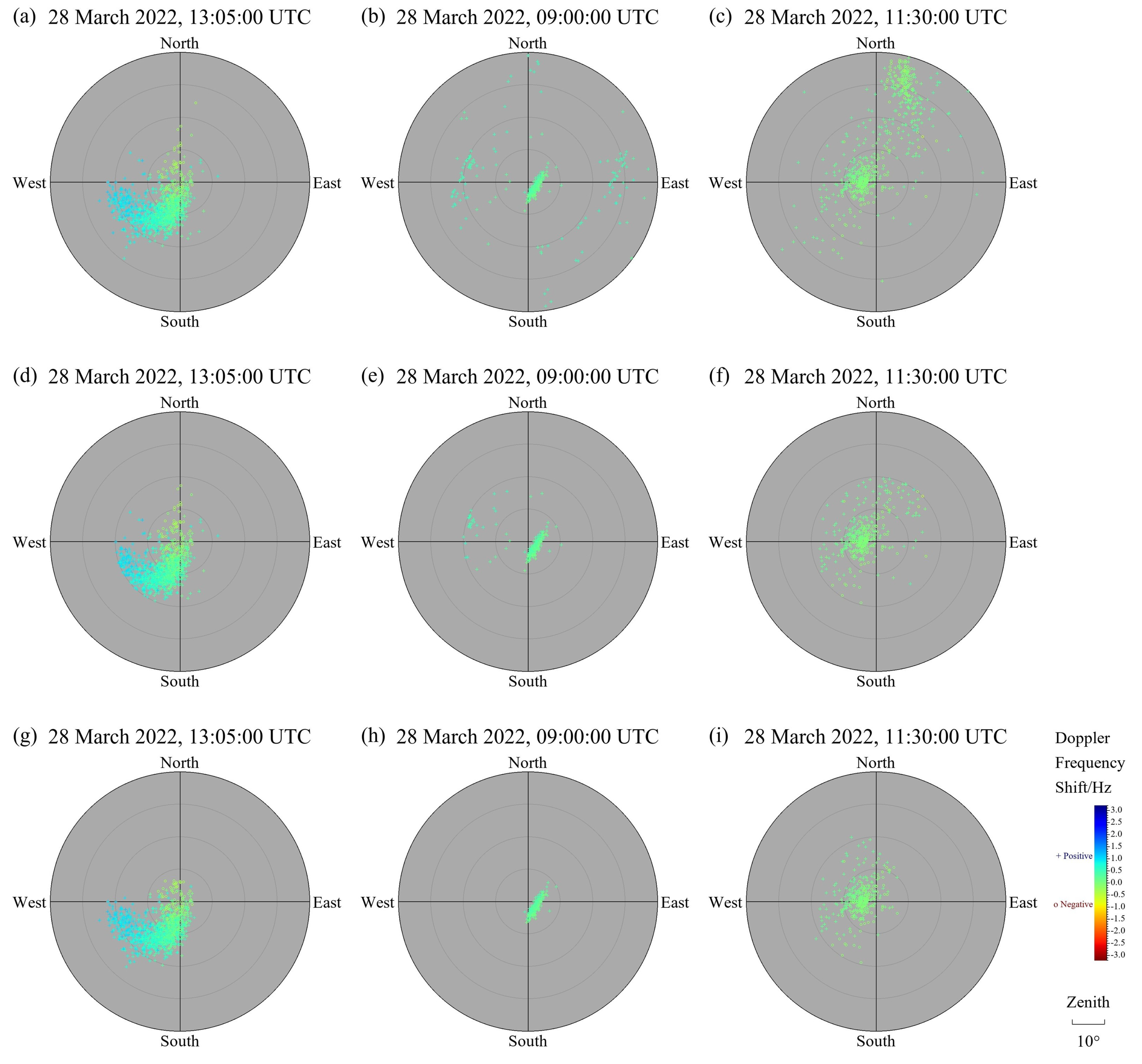
Plenty of F-region drift measurements such as those in Figure 6 show bipolar reflection clusters near vertical and whose maximum zenith angle is around 20°. The quality of reflection points can be further improved by limiting the maximum zenith angle at the expense of decreasing the calculation precision of horizontal velocity [30]. Experiments show that the quality of reflection points is improved somewhat by limiting the maximum zenith angle to 20° (Figure 6d–f), but this is not completely applicable to Figure 6b,c. Furthermore, the fitted drift velocity is more accurate and robust with a skymap whose reflection points are disturbed in a wider area.
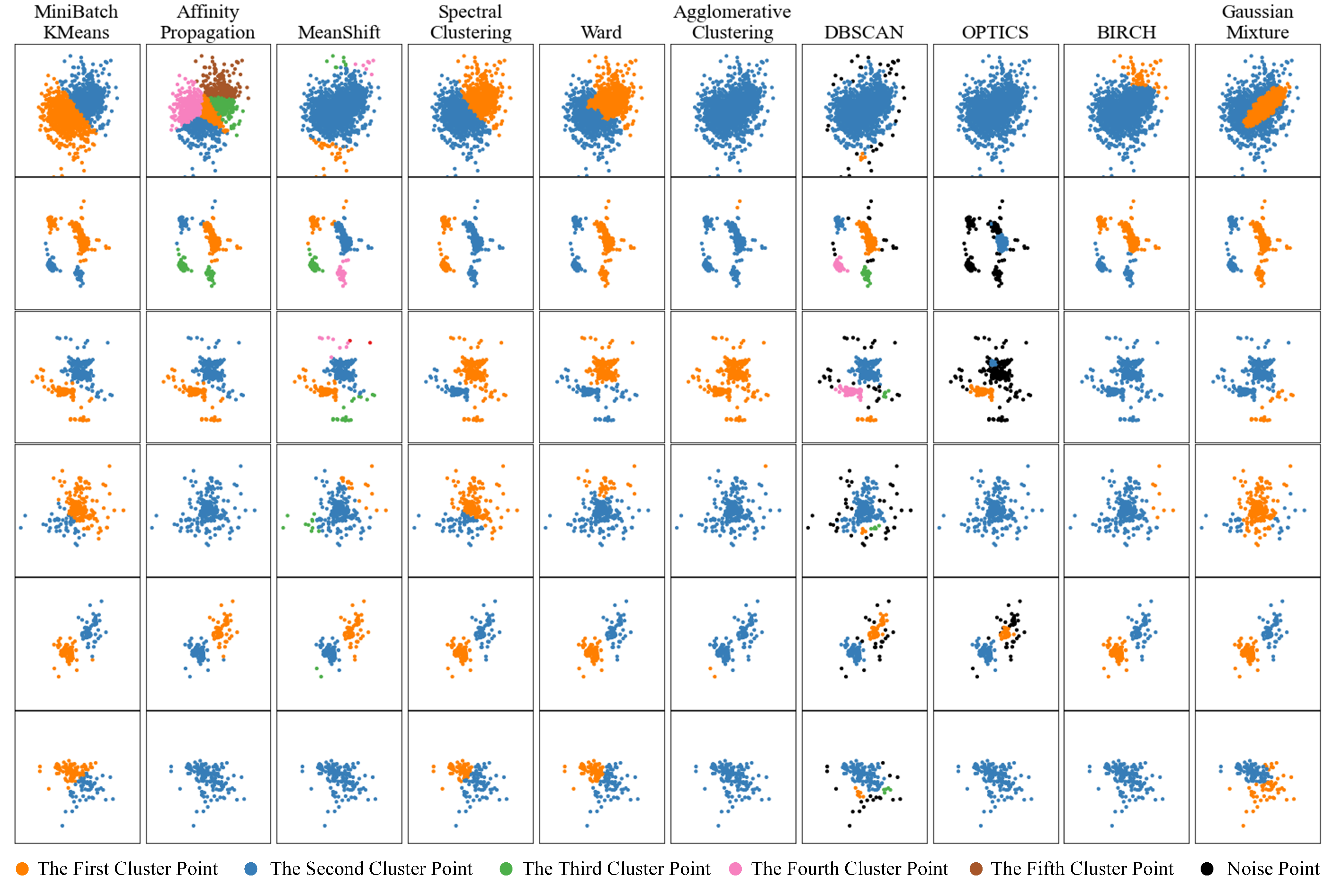
To improve this situation, ten clustering methods were used to cluster six representative skymaps. The clustering results in Figure 7 reveal that MeanShift, DBSCAN and OPTICS algorithms cluster better. These three methods are suitable for clustering the effective reflection points with a high-density distribution (concentrated distribution), as they are density-based clustering methods. The MeanShift algorithm finds and adjusts the centroid in accordance with the sample density in the dataset, whose location is the mean of the samples within its neighborhood [31]. DBSCAN and OPTICS algorithms look for high-density sample areas in the dataset and expand the surrounding areas into clusters. They differ in that the maximum distance between two samples in DBSCAN is a fixed value and the maximum distance between two samples in OPTICS is a value range [32,33,34]. These three clustering methods conduct clustering analysis on the basis of different criteria, and each has its own advantages and disadvantages. MeanShift and DBSCAN algorithms can more easily separate multiple clusters, but some scattered samples could be lost when there is only a single cluster; on the contrary, OPTICS makes it easier to retain all samples of a single cluster, while being able to roughly separate multiple clusters. If three clustering methods are combined for coarse clustering analysis, extracting the bipolar reflection cluster including selected reflection points can be easier and more effective. The following is the data processing process:
- (1)
- Set up the dataset. The number of samples X is the number of reflection points after Doppler filtering. The number of features Y being equal to two refers to the projection of reflection points in north–south and east–west directions.
- (2)
- MeanShift, DBSCAN and OPTICS algorithms are respectively used for clustering analysis on the dataset. When using a single clustering method to process data, the first priority is clustering. Subsequently, the clustering labels of all samples need to be extracted. Then, one solves the centroid of each cluster after removing the noise. Ultimately, the selected cluster embracing the centroid nearest to the center of skymap is the bipolar reflection cluster extracted by this single clustering method.
- (3)
- Vote out the reliable bipolar reflection cluster. The first step is splicing reflection clusters extracted by three clustering methods into a new dataset. Afterwards, by means of voting, the new cluster formed by extracted all reflection points with more votes from that dataset is the required bipolar reflection cluster.
Figure 6g–i show the distribution of reflection points after coarse clustering analysis. Coarse clustering can extract the higher quality bipolar reflection cluster and ensure the accuracy of drift velocity while reducing the calculation precision of horizontal velocity. Generally speaking, coarse clustering analysis can avoid uncontrollable measurement errors caused by ionospheric fluctuation and system error, which provides strong backing for actualizing the automatic and high-quality drift measurement. In addition, the numbers of reflection points and the drift velocity components of the cases in Figure 6 are shown in Table 1, Table 2 and Table 3.
3.4. Calculating the Drift Velocity
Theoretically, all primary echo reflection points satisfy Equation (6). Nevertheless, not all points can indeed satisfy that. Consequently, the WLS method considered to fit the sub-drift velocity is:
where is the number of all reflection points within the bipolar reflection cluster ultimately used to fit drift velocity; I is the number of its subset; and , and are components of the sub-drift velocity . The larger the Doppler frequency shift value is, the lower its reliability. Naturally, the weighting factor can be introduced into the error index . For the i-th point, its weighting factor is negatively correlated with its Doppler frequency shift value:
where is the maximum Doppler frequency shift value.
When using the WLS method to fit the drift velocity, each subset of reflection points included in the bipolar reflection cluster should be used to fit a sub-drift velocity. Start with a subset of I (at least three) reflection points and calculate the sub-drift velocity ; then add another reflection point to the previous subset, forming a new subset to calculate the sub-drift velocity ; and then for a while, repeat the previous step until the sub-drift velocity is calculated using all reflection points. The drift velocity is the mean of sub-drift velocities. The standard deviation of sub-drift velocities can evaluate the uncertainty of drift velocity measurement. If the plasma moves uniformly in the sampling period and the filtering effect of reflection points is excellent, all sub-drift velocities should be similar; thus, the sub-drift velocity distribution is relatively narrow and the uncertainty is quite small. Otherwise, the sub-drift velocity distribution becomes wider and the uncertainty becomes larger.
4. Experimental Results
Four experiments were conducted in Hainan Station (geographic coordinates 19.4°N, 109.0°E) for verifying the automatic drift-measurement-data-processing method. Nearly ten thousand drift measurements were processed in 2021–2022. To better compare experimental results, the DPS4D ionosonde is positioned 60 m southeast of the CAS-DIS ionosonde. Both devices have the same antenna layout. Two ionosonde systems perform drift detection every 5 min. DPS4D and CAS-DIS need interlaced drift detection so that the mutual interference between them can be reduced. The reliability and wide applicability of the new method can be verified by using the two methods to process drift echo data received by the two systems.
The first experiment only adopted drift echo data of DPS4D system which were measured from 11 June 2021 to 23 June 2021. The automatic drift-measurement-data-processing method proposed in this paper (the new method) was used to process drift echo data. Then, the obtained drift velocities were compared with the drift velocities which had been calculated by the previous method encapsulated inside DPS4D system. The comparison results present that they have high similarity, and the newly obtained drift velocities change more gently and have smaller standard deviations. These further indicate that unreliable reflection points are eliminated or reduced, rapid fluctuations of drift velocities are retarded appropriately and the quality of drift measurements is improved. Figure 8 shows a comparison of drift velocities from 11 June 2021 to 12 June 2021. This experiment proves the feasibility of the drift data processing method proposed in this paper and illustrates that this new method is suitable for the DPS4D system.
In the second experiment and the third experiment, the CAS-DIS system received its own drift echo data and ran automatic drift-measurement-data-processing method (the new method), and the DPS4D system also received its own drift echo data and ran its own data processing method (the previous method). Due to the fact that the detection objects are drift velocities in the same ionospheric region, the results that they have similar drift velocity variation trends are reasonable. A fine comparison of drift measurements of two systems is indeed unreliable, but it can be demonstrated that the new method is also applicable to the CAS-DIS system by obtaining similar drift velocity variation trends, and the obtained drift measurements can be used to calibrate and analyze each other.
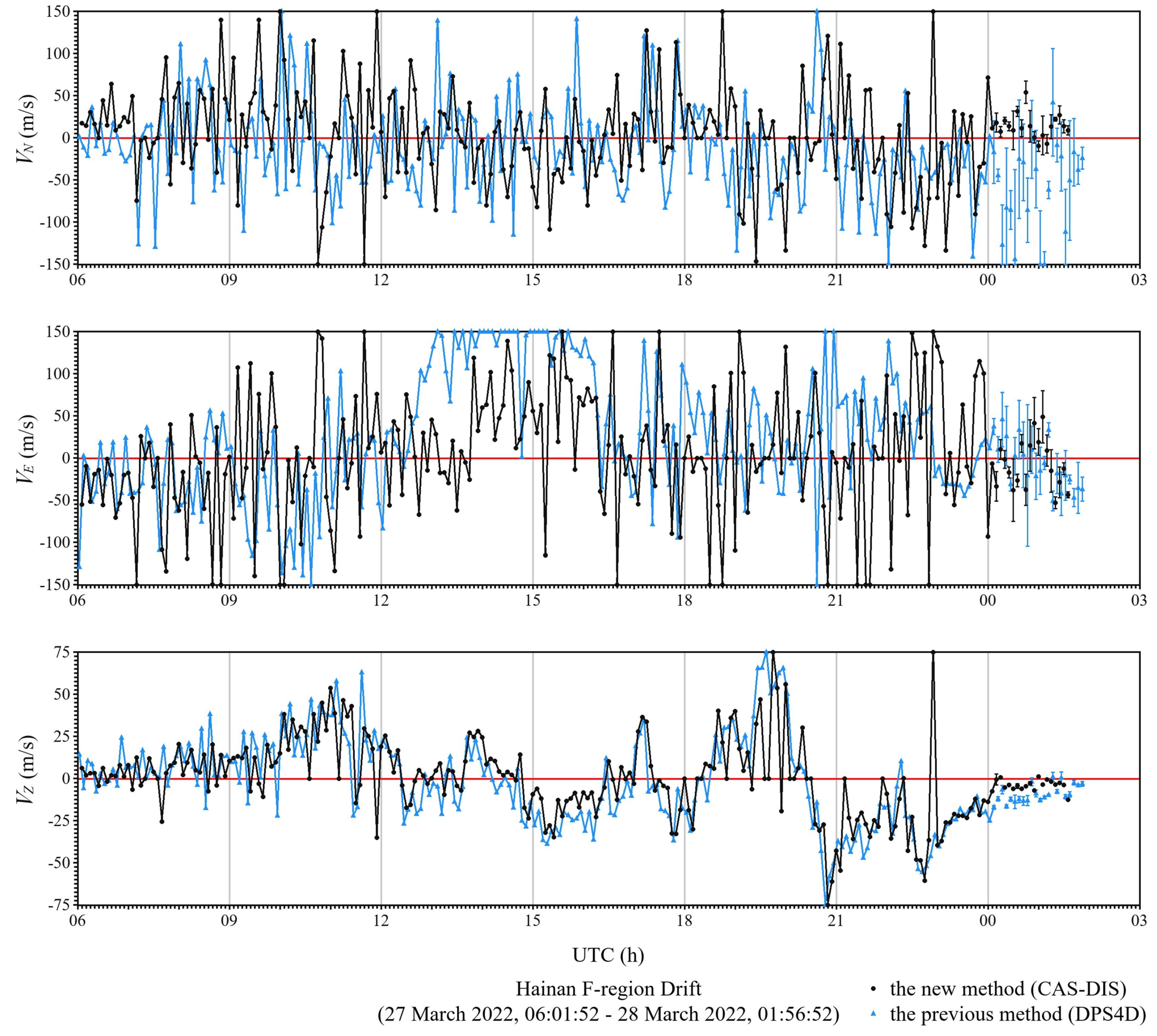
The second experiment (Figure 9) was conducted from 27 March 2022 to 28 March 2022. For the CAS-DIS system, its every vertical detection is 3 min earlier than that of every drift detection event. Here are its working parameters in drift detection mode. Pulse train signals of four frequencies are transmitted. A single frequency pulse signal is transmitted 500 times. The pulse repetition interval (PRI) is 50 ms. Figure 10a shows the transmitting sequence of its drift detection. As the receiving sampling sequence is completed in accordance with transmitting sequence, the data sampling period is 50 ms, the sampling rate is 20 Hz and the Doppler resolution is up to 0.04 Hz.
Since the previous method owned by the DPS4D system does not dynamically restrict the optimal height range based on the adjacent ionogram when restricting the ionospheric detection region, on 27 March 2022, 13:02:02–15:37:02, reflection points from primary and secondary echoes were used for fitting the drift velocity. These drift velocities are distortions in that the reflection points from the secondary echoes are distributed in the east–west direction. On 28 March 2022, 00:00:00–01:56:52, since the previous method owned by the DPS4D system extracted the unreliable reflection cluster, reflection points included the reliable reflection cluster and time invariant reflection clusters. The standard deviations of these fitted drift velocities are larger than the standard deviations of that drift velocities obtained by the new method owned by the CAS-DIS system. The components of drift velocities have highly similar variation trends in the drift measurement results of the CAS-DIS system and DPS4D system, which verifies the validity of the proposed new method.
The third experiment was conducted from 28 March 2022 to 10 April 2022. In drift detection, what differed from the second experiment was that CAS-DIS system adopted frequency multiplexing (FM), transmitted pulse train signals of five frequencies and transmitted a single frequency pulse signal 400 times. The PRI was still 50 ms. Figure 10b shows the transmitting sequence of its drift detection, which is essentially another mode of drift detection. Hence, the single-frequency repetition interval was 250 ms, the sampling rate was 4 Hz and the Doppler resolution was increased to 0.01 Hz. By improving the Doppler resolution, FM could avoid the strong interference at the high Doppler frequencies.
The similarity was also sustained by comparing drift measurement results of CAS-DIS and DPS4D from 28 March 2022 to 29 March 2022 (Figure 11). On 28 March 2022, 11:26:52–14:17:02, reflection points from primary and secondary echoes were used for fitting the drift velocity. On account of the reflection points from the secondary echoes distributed in the north–south direction, these drift velocities are distortions. On 28 March 2022, 21:02:02–22:16:52, there was a partial overlap between the E and F layers, and the strong E layer echoes blocked all or part of the F layer echoes. From 28 March 2022, 23:00:00 to 29 March 2022, 05:00:00, the method owned by DPS4D extracted the unreliable reflection points, including the reliable reflection cluster and time invariant reflection clusters. The standard deviations of these drift velocities are larger than the standard deviations of the drift velocities obtained by the new method owned by the CAS-DIS system. It can be demonstrated that the new method is also applicable to CAS-DIS with another drift detection mode, and this further demonstrates the wide applicability of the new method. Combined with the results of the second experiment and the third experiment, the diurnal variation of drift velocities can be observed.
Since drift velocities are affected by the solar activities, the diurnal variation law of drift velocities exists. In the last experiment, in order to better observe whether drift velocities had a diurnal variation law, we statistically analyzed the drift velocities processed by CAS-DIS which had been obtained in the third experiment. Figure 12 shows the statistical results of drift velocities from 7 April 2022 to 10 April 2022, which reveals the plain diurnal variation.
What should be clear from these experiments is that the parameter settings do not need to constantly change as external conditions change when the new method process the drift echo data. Note that some outlier values in drift velocity statistics were caused by a few reflection points or wrong automatic calibration results of the ionogram.
5. Discussion
In this paper, an automatic drift-measurement-data-processing method was presented that can effectively improve the drift measurement ability of a digital ionosonde. Based on Doppler interferometry, this method filters clutter step by step, and optimizes drift measurement quality through multiple constraints. Consequently, this constrained data processing method provides strong support for realizing automatic drift measurement and obtaining reliable drift measurement results. Additionally, its data processing cycle can be divided into four stages: extracting the stable echo data, restricting the ionospheric detection region, extracting the reliable reflection cluster and calculating the drift velocity.
In the first stage, extracting the stable echo data is essentially data preprocessing. We extract reliable O-wave data as data processing objects (echo data); improve SNR by complementary code pulse compression; and reduce echo fluctuation and suppress interference by median filtering and other data preprocessing techniques. The extracted echo data are essential and useful for obtaining accurate and obtaining stable drift measurement results. Ultimately, the information of preprocessed echo data includes amplitudes, phases, virtual heights, echo directions and Doppler frequency shifts.
In the second stage, we select the optimal height range to restrict the ionospheric detection region. It is especially necessary to use a recently acquired ionogram to determine the detection frequencies and the optimal height range. Compared with the correct drift measurement results, if the ionosphere has obvious E and F layers, the false optimal height range could produce obviously different reflection clusters, resulting in serious distortion of drift measurement results; if the detection frequency is higher than the ionospheric plasma frequency, no effective reflection points could be extracted from the false echo information, resulting in serious distortion of drift measurement results (Figure 3).
In the third stage, the Doppler filtering and coarse clustering analysis aim to obtain a reliable reflection cluster. It is essential to carry out Doppler filtering according to the spectral characteristics of the echoes. The Doppler filtering can not only filter white noise, but also effectively remove strong random external interference. For example, in the last three experiments, the CAS-DIS system could receive part of the transmitted signals of the DPS4D system when receiving signals. After Doppler filtering, the strong reflection points belonging to DPS4D can be filtered out, and the distribution of these strong reflection points is similar to the distribution of reflection points obtained by the DPS4D system when it conducts drift detection in near real-time. In this paper, coarse clustering analysis was introduced into drift measurement data processing for the first time. It can extract the reflection cluster near the center of a skymap with a high-density distribution, further enhancing the capacity of automatic drift measurement. As can be seen in Figure 6, reflection points with small Doppler frequency shift values far from the center of the skymap can decrease the estimated drift velocity and result in weakening the capacity of drift measurement. This constrained stage can solve the problem of some reflection points with small Doppler shifts being far away from the center of skymap, which exist during certain periods of daytime.
The last stage uses the WLS method for calculating the drift velocity. The introduction of a weighting factor further reduces the influence of reflection points with high Doppler frequency shifts on the drift velocity. Figure 8, Figure 9, Figure 10, Figure 11 and Figure 12 indicate that drift velocities have diurnal variation and have similar variation trends in the CAS-DIS system and DPS4D system, which further verifies the feasibility of this method for more than one digital ionosonde. However, a few reflection points will degrade the quality of drift measurement, which could be considered to break through in future research.
6. Conclusions
Providing real-time and long-term ionospheric plasma drift state information is highly desirable. Summarizing this constrained method is valuable for future research on the data processing of drift measurements. This automatic drift-measurement-data-processing method can automatically complete high-quality drift measurements without constantly changing parameter settings as external conditions change, and is suitable for the CAS-DIS system, the DPS4D system and other digital ionosonde systems. Currently, this method has been successfully applied to the CAS-DIS system, and it will be used in more observation stations to perform long-term, automatic and high-quality drift measurements in the future. We hope this method will motivate ionospheric plasma motion research.
Author Contributions
Conceptualization, X.M., Z.G. and F.Z.; methodology, X.M. and F.Z.; software, X.M., Z.G. and S.W.; validation, X.M., Z.G. and F.Z.; formal analysis, X.M. and X.L.; investigation, G.F. and X.L.; resources, G.F., F.Z. and S.W.; data curation, Z.G. and F.Z.; writing—original draft preparation, X.M.; writing—review and editing, Z.G. and F.Z.; visualization, X.M.; supervision, G.F.; project administration, X.L. and S.W.; funding acquisition, G.F. All authors have read and agreed to the published version of the manuscript.
Funding
This research was funded by the National Nature Science Foundation of China, grant number 61827803.
Conflicts of Interest
The authors declare no conflict of interest.
References
- Mikhailov, A.V.; Perrone, L.; Nusinov, A.A. Mid-Latitude Daytime F2-Layer Disturbance Mechanism under Extremely Low Solar and Geomagnetic Activity in 2008–2009. Remote Sens. 2021, 13, 1514. [Google Scholar] [CrossRef]
- Ghasemi, A.; Abedi, A.; Ghasemi, F. Propagation Engineering in Wireless Communications; Springer: New York, NY, USA, 2012; pp. 127–206. ISBN 978-1-4614-1076-8. [Google Scholar]
- Beach, T.L.; Kintner, P.M. Development and use of a GPS ionospheric scintillation monitor. IEEE Trans. Geosci. Remote Sens. 2001, 39, 918–928. [Google Scholar] [CrossRef]
- Reinisch, B.W.; Galkin, I.A.; Khmyrov, G.M.; Kozlov, A.V.; Lisysyan, I.A.; Bibl, K.; Cheney, G.; Kitrosser, D.; Stelmash, S.; Roche, K.; et al. Advancing digisonde technology: The DPS-4D. AIP Conf. Proc. 2008, 974, 127–143. [Google Scholar] [CrossRef]
- Wang, S.; Chen, Z.; Zhang, F.; Gong, Z.; Fang, G. A new design for digital ionosonde. Chin. J. Space Sci. 2014, 34, 849–857. [Google Scholar] [CrossRef]
- Branitskii, A.V.; Kim, V.Y.; Polimatidi, V.P. Rapid Variations in Electron Density Profiles in the Ionosphere Detected with the Izmiran High-Speed Ionosonde. Geomagn. Aeron. 2020, 60, 63–79. [Google Scholar] [CrossRef]
- Shindin, A.V.; Moiseev, S.P.; Vybornov, F.I.; Grechneva, K.K.; Pavlova, V.A.; Khashev, V.R. The Prototype of a Fast Vertical Ionosonde Based on Modern Software-Defined Radio Devices. Remote Sens. 2022, 14, 547. [Google Scholar] [CrossRef]
- Ke, K.J.; Su, C.L.; Kuong, R.M.; Chen, H.C.; Lin, H.S.; Chiu, P.H.; Ko, C.Y.; Chu, Y.H. New Chung-Li Ionosonde in Taiwan: System Description and Preliminary Results. Remote Sens. 2022, 14, 1913. [Google Scholar] [CrossRef]
- Briggs, B.H.; Phillips, G.J.; Shinn, D. The Analysis of Observations on Spaced Receivers of the Fading of Radio Signals. Proc. Phys. Soc. B 1950, 63, 106. [Google Scholar] [CrossRef]
- Fooks, G.F.; Jones, I.L. Correlation analysis of the fading of radio waves reflected vertically from the ionosphere. J. Atmos. Sol. Terr. Phys. 1961, 20, 229–242. [Google Scholar] [CrossRef]
- Reinisch, B.W.; Scali, J.L.; Haines, D.L. Ionospheric drift measurements with ionosondes. Ann. Geophys. 1998, 41, 695–702. [Google Scholar] [CrossRef]
- Wright, J.W.; Pitteway, M.L.V. High-resolution vector velocity determinations from the dynasonde. Atmos. Terr. Phys. 1994, 56, 961–977. [Google Scholar] [CrossRef]
- Bianchi, C.; Altadill, D. Ionospheric Doppler measurements by means of HF-radar techniques. Ann. Geophys. 2005, 48, 989–993. [Google Scholar] [CrossRef]
- Morris, R.J.; Monselesan, D.P.; Hyde, M.; Breed, A.M.; Wilkinson, P.J. Southern polar cap DPS and CADI ionosonde measurements: 2. F-region drift comparison. Adv. Space Res. 2004, 33, 937–942. [Google Scholar] [CrossRef]
- Bullett, T.W. Mid-Latitude Ionospheric Plasma Drift: A Comparison of Digital Ionosonde and Incoherent Scatter Radar Measurements at Millstone Hill; University of Massachusetts Lowell: Lowell, MA, USA, 1994. [Google Scholar]
- Fejer, B.G.; de Paula, E.R.; Batista, I.S.; Bonelli, E.; Woodman, R.F. Equatorial F region vertical plasma drifts during solar maxima. J. Geophys. Res. 1989, 94, 12049–12054. [Google Scholar] [CrossRef]
- Scali, J.L.; Reinisch, B.W.; Heinselman, C.J.; Bullett, T.W. Coordinated digisonde and incoherent scatter radar F region drift measurements at Sondre Stromfjord. Radio Sci. 1995, 30, 1481–1498. [Google Scholar] [CrossRef]
- Sedgemore, K.J.F.; Wright, J.W.; Williams, P.J.S.; Jones, G.O.L.; Rietveld, M.T. Plasma drift estimates from the Dynasonde: Comparison with EISCAT measurements. Ann. Geophys. 1998, 16, 1138–1143. [Google Scholar] [CrossRef]
- Woodman, R.F.; Chau, J.L.; Ilma, R.R. Comparison of ionosonde and incoherent scatter drift measurements at the magnetic equator. Geophys. Res. Lett. 2006, 33, L01103. [Google Scholar] [CrossRef]
- Huang, L.; Wen, B.; Wu, L.; Yao, M. Ionospheric interference mitigation in HFSWR. Chin. J. Radio Sci. 2007, 22, 626–630. [Google Scholar] [CrossRef]
- Chen, G.; Zhao, Z.; Zhu, G.; Huang, Y.; Li, T. Hf radio-frequency interference mitigation. IEEE Geosci. Remote. Sens. Lett. 2010, 7, 479–482. [Google Scholar] [CrossRef]
- Chen, K.; Zhu, Z.; Ning, B.; Lan, J.; Sun, F. Radio frequency interference mitigation algorithm in ionosonde. Chin. J. Radio Sci. 2013, 28, 391–396. [Google Scholar]
- Liu, T.; Yang, G.; Hu, Y.; Jiang, C.; Lan, T.; Zhao, Z.; Ni, B. A Novel Ionospheric Sounding Network Based on Complete Complementary Code and Its Application. Sensors 2019, 19, 779. [Google Scholar] [CrossRef] [PubMed] [Green Version]
- Wang, S.; Chen, Z.; Zhang, F.; Gong, Z.; Li, J.; Fang, G. A method for separating O-wave and X-wave and its application in digital ionosonde. Ann. Geophys. 2013, 56, A0567. [Google Scholar] [CrossRef]
- Igi, S.; Minakoshi, H.; Yoshida, M. Automatic ionogram processing system. II: Automatic ionogram scaling. J. Commun. Res. Lab. 1992, 39, 367–379. [Google Scholar]
- Reinisch, B.W.; Huang, X.; Galkin, I.A.; Paznukhov, V.; Kozlov, A. Recent advances in real-time analysis of ionograms and ionospheric drift measurements with digisondes. J. Atmos. Sol. Terr. Phys. 2005, 67, 1054–1062. [Google Scholar] [CrossRef]
- Pezzopane, M.; Scotto, C. Automatic scaling of critical frequency foF2 and MUF(3000)F2: A comparison between Autoscala and ARTIST 4.5 on Rome data. Radio Sci. 2007, 42, RS4003. [Google Scholar] [CrossRef]
- Galkin, I.A.; Khmyrov, G.M.; Kozlov, A.V.; Reinisch, B.W.; Huang, X.; Paznukhov, V.V. The ARTIST 5. AIP Conf. Proc. 2008, 974, 150. [Google Scholar] [CrossRef]
- Kouba, D.; Knížová, P.K. Analysis of digisonde drift measurements quality. J. Atmos. Sol. Terr. Phys. 2012, 90–91, 212–221. [Google Scholar] [CrossRef]
- Kouba, D.; Boška, J.; Galkin, I.A.; Santolík, O.; Šauli, P. Ionospheric drift measurements: Skymap points selection. Radio Sci. 2008, 43, RS1S90. [Google Scholar] [CrossRef]
- Comaniciu, D.; Meer, P. Mean shift: A robust approach toward feature space analysis. IEEE Trans. Pattern Anal. Mach. Intell. 2002, 24, 603–619. [Google Scholar] [CrossRef]
- Ankerst, M.; Breunig, M.M.; Kriegel, H.P.; Sander, J. OPTICS: Ordering points to identify the clustering structure. SIGMOD Rec. 1999, 28, 49–60. [Google Scholar] [CrossRef]
- Ester, M.; Kriegel, H.P.; Sander, J.; Xu, X. A Density-Based Algorithm for Discovering Clusters in Large Spatial Databases with Noise. In Proceedings of the 2nd International Conference on Knowledge Discovery and Data Mining (KDD’96), Portland, OR, USA, 2–4 August 1996; pp. 226–231. [Google Scholar]
- Schubert, E.; Sander, J.; Ester, M.; Kriegel, H.P.; Xu, X. DBSCAN revisited, revisited: Why and how you should (still) use DBSCAN. ACM Trans. Database Syst. 2017, 42, 1–21. [Google Scholar] [CrossRef]
Figure 1.
Autocorrelation processing results of complementary codes and sum result of two autocorrelation functions.
Figure 1.
Autocorrelation processing results of complementary codes and sum result of two autocorrelation functions.

Figure 2.
Schematic diagram of the drift measurement information.

Figure 3.
Demonstration of detection frequency selection and optimal height range restriction. (a) Invalid drift measurement results with no reasonable detection frequencies. (b) Invalid drift measurement results with reasonable detection frequencies but no reasonable optimal height range. (c) Valid drift measurement results with reasonable detection frequencies and a reasonable optimal height range. (d) Ionogram obtained 3 min before drift measurement (a). (e) Ionogram obtained 3 min before drift measurement (b,c).

Figure 4.
Doppler spectrum at a single detection frequency point and single height.

Figure 5.
Case of Doppler filtering. (a) Distribution of reflection points after ionospheric detection region restriction. (b) Distribution of reflection points filtered by the amplitude threshold in Doppler filtering. (c) Distribution of reflection points filtered by Doppler frequency shift threshold in Doppler filtering.

Figure 6.
Cases of coarse clustering analysis. (a–f) No coarse clustering analysis. (a–c) Raw method: the maximum zenith angle is 40°. (d–f) Corrected Method 1: slightly improving the quality of reflection points by reducing maximum the zenith angle to 20°. (g–i) Corrected Method 2: effectively improving the quality of reflection points by applying coarse clustering analysis and maintaining the maximum zenith angle at 40°.

Figure 7.
Clustering analysis results of ten clustering methods.

Figure 8.
Statistics of the F-region drift velocity in Hainan from 11 June 2021, 00:00:00 to 12 June 2021, 00:00:00 in UTC.
Figure 8.
Statistics of the F-region drift velocity in Hainan from 11 June 2021, 00:00:00 to 12 June 2021, 00:00:00 in UTC.

Figure 9.
Statistics of the F-region drift velocity in Hainan from 27 March 2022, 06:01:52 to 28 March 2022, 01:56:52 in UTC.
Figure 9.
Statistics of the F-region drift velocity in Hainan from 27 March 2022, 06:01:52 to 28 March 2022, 01:56:52 in UTC.

Figure 10.
Transmitting sequence of drift detection of CAS-DIS. (a) The second experiment; (b) the third experiment and the last experiment.
Figure 10.
Transmitting sequence of drift detection of CAS-DIS. (a) The second experiment; (b) the third experiment and the last experiment.

Figure 11.
Statistics of the F-region drift velocity in Hainan from 28 March 2022, 05:00:00 to 29 March 2022, 05:00:00 in UTC.
Figure 11.
Statistics of the F-region drift velocity in Hainan from 28 March 2022, 05:00:00 to 29 March 2022, 05:00:00 in UTC.

Figure 12.
Statistics of the F-region drift velocity in Hainan from 7 April 2022, 00:00:00 to 10 April 2022, 00:00:00 in UTC.
Figure 12.
Statistics of the F-region drift velocity in Hainan from 7 April 2022, 00:00:00 to 10 April 2022, 00:00:00 in UTC.


Table 1.
Numbers of reflection points and drift velocity components obtained by raw method, corrected method 1 and corrected method 2 on 28 March 2022, 13:05:00 UTC.
Table 1.
Numbers of reflection points and drift velocity components obtained by raw method, corrected method 1 and corrected method 2 on 28 March 2022, 13:05:00 UTC.
| Data Processing | Number of Reflection Points | |||
|---|---|---|---|---|
| Raw Method | 1147 | |||
| Corrected Method 1 | 1078 | |||
| Corrected Method 2 | 1119 |
Table 2.
Numbers of reflection points and drift velocity components obtained by raw method, corrected method 1 and corrected method 2 on 28 March 2022, 09:00:00 UTC.
Table 2.
Numbers of reflection points and drift velocity components obtained by raw method, corrected method 1 and corrected method 2 on 28 March 2022, 09:00:00 UTC.
| Data Processing | Number of Reflection Points | |||
|---|---|---|---|---|
| Raw Method | 591 | |||
| Corrected Method 1 | 495 | |||
| Corrected Method 2 | 458 |
Table 3.
Numbers of reflection points and drift velocity components obtained by raw method, corrected method 1 and corrected method 2 on 28 March 2022, 11:30:00 UTC.
Table 3.
Numbers of reflection points and drift velocity components obtained by raw method, corrected method 1 and corrected method 2 on 28 March 2022, 11:30:00 UTC.
| Data Processing | Number of Reflection Points | |||
|---|---|---|---|---|
| Raw Method | 611 | |||
| Corrected Method 1 | 377 | |||
| Corrected Method 2 | 335 |
Publisher’s Note: MDPI stays neutral with regard to jurisdictional claims in published maps and institutional affiliations. |
© 2022 by the authors. Licensee MDPI, Basel, Switzerland. This article is an open access article distributed under the terms and conditions of the Creative Commons Attribution (CC BY) license (https://creativecommons.org/licenses/by/4.0/).
Share and Cite
MDPI and ACS Style
Ma, X.; Gong, Z.; Zhang, F.; Wang, S.; Liu, X.; Fang, G. An Automatic Drift-Measurement-Data-Processing Method with Digital Ionosondes. Remote Sens. 2022, 14, 4710. https://0-doi-org.brum.beds.ac.uk/10.3390/rs14194710
AMA Style
Ma X, Gong Z, Zhang F, Wang S, Liu X, Fang G. An Automatic Drift-Measurement-Data-Processing Method with Digital Ionosondes. Remote Sensing. 2022; 14(19):4710. https://0-doi-org.brum.beds.ac.uk/10.3390/rs14194710
Chicago/Turabian StyleMa, Xiaoya, Zhaoqian Gong, Feng Zhang, Shun Wang, Xiaojun Liu, and Guangyou Fang. 2022. "An Automatic Drift-Measurement-Data-Processing Method with Digital Ionosondes" Remote Sensing 14, no. 19: 4710. https://0-doi-org.brum.beds.ac.uk/10.3390/rs14194710
Note that from the first issue of 2016, this journal uses article numbers instead of page numbers. See further details here.