
Multiscale Superpixel Guided Discriminative Forest for Hyperspectral Anomaly Detection


1
School of Aerospace Science and Technology, Xidian University, Xi’an 710126, China
2
Shaanxi Academy of Aerospace Technology Application Co., Ltd., Xi’an 710199, China
*
Author to whom correspondence should be addressed.
Remote Sens. 2022, 14(19), 4828; https://0-doi-org.brum.beds.ac.uk/10.3390/rs14194828
Submission received: 23 August 2022
/
Revised: 20 September 2022
/
Accepted: 23 September 2022
/
Published: 27 September 2022
(This article belongs to the Special Issue Theory and Application of Machine Learning in Remote Sensing)
Abstract
:Recently, the isolation forest (IF) methods have received increasing attention for their promising performance in hyperspectral anomaly detection (HAD). However, limited by the ability of exploiting spatial-spectral information, existing IF-based methods suffer from a lot of false alarms and disappointing performance of detecting local anomalies. To overcome the two problems, a multiscale superpixel guided discriminative forest method is proposed for HAD. First, the multiscale superpixel segmentation is employed to generate some homogeneous regions, and it can effectively extract spatial information to guide anomaly detection for the discriminative forest in local areas. Then, a novel discriminative forest (DF) model with the gain split criterion is designed, which enhances the sensitivity of the DF to local anomalies by the utilization of multi-dimension spectral bands for node division; meanwhile, the acceptable range of hyperplane attribute values is introduced to capture any unseen anomaly pixels that are out-of-range in the evaluation stage. Finally, for the high false alarm rate situation in the existing IF-based algorithms, the multiscale fusion with guided filtering is put forward to refine the initial detection results from the DF. In addition, the extensive experimental results on four real hyperspectral datasets demonstrate the effectiveness of the proposed method.
1. Introduction
Hyperspectral images (HSIs) have abundant spectral information of geographical materials, which is different from the traditional optical and spectral images, and this feature makes different ground targets more discriminative. Accordingly, the HSI derives many research directions, such as target detection [1,2], anomaly detection [3,4], band selection [5,6], hyperspectral unmixing [7], hyperspectral denoising [8,9], etc.
Hyperspectral anomaly detection (HAD) [10,11] is a challenging task in hyperspectral image (HSI) processing, and its key purpose is to capture anomaly targets from the background by the utilization of spectral and spatial differences with no prior knowledge. Benefiting from the above characteristic, the HAD is widely used in civil and military applications.
The isolation forest (IF) methods [12] are attracting more attention to the HAD in the last three years, which take advantage of the fact that anomalies are “few and different” in a given HSI, thus anomaly pixels are more susceptible to be isolated than background pixels during the construction processing of an isolation forest. To be specific, Li et al. [13] propose the kernel isolation forest detection (KIFD) method, which combines the kernel principal component analysis (KPCA) with the IF to obtain the initial detection maps, then the iteration strategy is applied to refine the detection results. Afterward, a novel isolation forest method based on multiple features (MFIFD) [14] is proposed for HAD. The multiple features including the Gabor, extend morphological profile (EMP), extend multi-attribute profile (EMAP) and spectral features are applied to build isolation forest to improve the detection accuracy. To better define a pixel as an anomaly or background, a subspace selection-based discriminative forest (SSDF) [15] is put forward.
Although the above IF-based methods have achieved a good effect in the HAD, these methods still have two deficiencies, i.e., the poor performance of detecting local anomalies and a high false alarm rate (FAR), due to the limited utilization capacity of HSI spectral-spatial information. The two problems are analyzed from the angles of methodology and detection results. In the methodology, the IF-based methods usually adopt the path length in the global samples to measure the anomaly degree of test pixels [16], but the essence of anomalies in an HSI is that the anomaly degree of each pixel depends on the difference among its surrounding pixels. By comparison, the global way in the IF-based methods does not correspond with the anomaly essence and ignores the discriminability of anomalous pixels in local spatial areas. Furthermore, using an individual spectral band is not very effective in each node partition of isolation trees. Consequently, these two points lead to poor performance in detecting local anomalies. On the other hand, the IF-based methods in HSI complex scenes ignore the importance of spatial features and cannot distinguish the background pixels well, resulting in suffering from a lot of false alarms. From the perspective of detection results, the anomaly detection maps are shown in Figure 1, and the SSDF and KIFD methods are the isolation forest methods. It is obvious that the SSDF method has poor performance in detecting local anomalies. To be specific, as is shown in Figure 1c, the SSDF method is not able to detect well anomaly targets which are several buildings in the upper left corner. In addition, the SSDF and KIFD methods always erroneously detect the green background pixels as anomalies, causing a lot of false alarms, especially the KIFD method.
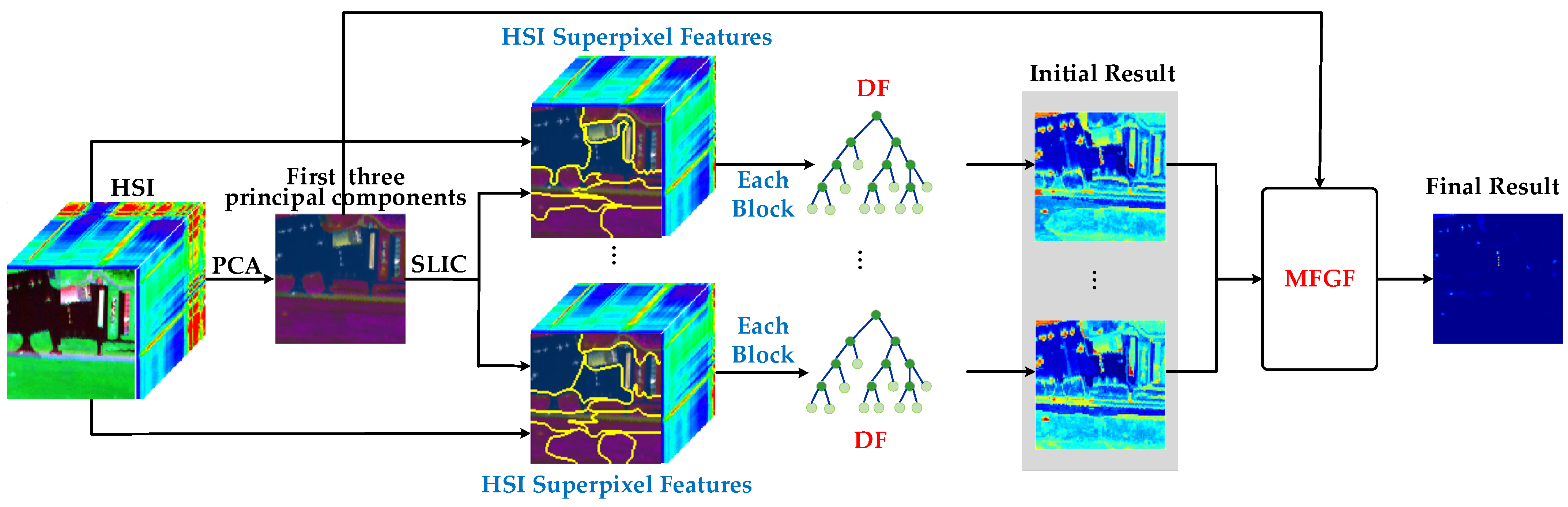
In order to solve the two problems, the multiscale superpixel guided discriminative forest (MSGDF) algorithm is proposed in Figure 2. The major contributions are as follows.
- (1)
- The strategy of multiscale superpixel guided discrimination forest is proposed for hyperspectral anomaly detection in this article. Concretely, the multiscale superpixel segmentation is adopted to mine HSI spatial information and make anomalies more discriminative in local areas, which can better guide the detection of local anomalies for DF.
- (2)
- A novel discriminative forest (DF) is designed. On the one hand, a gain split criterion based on multi-dimension spectral bands is utilized to make the DF more sensitive to anomaly pixels; On the other hand, the acceptable range of hyperplane attribute values is introduced to capture any unseen anomaly pixels that are out-of-range in the evaluation stage.
- (3)
- Aiming at the problem of high false alarm rates in the existing IF-based methods, the multiscale fusion with guided filtering (MFGF) module is put forward in the paper, which integrates multiscale detection maps with different spatial features to refine the initial DF results.
- (4)
- Compared with the state-of-the-art algorithms, the experimental results on four HSI datasets demonstrate the superiority of the proposed method.
2. Related Work
Many HAD methods have been developed in the past few decades [10]. One of the most classical algorithms is the Reed–Xiaoli (RX) [17], which proposes the hypothesis that the background features obey the Gaussian multivariate distribution, and the mean vector and covariance matrix of the whole HSI pixels are employed to represent the background, then the Mahalanobis distance is applied to measure the anomaly degree of test pixels. Whereas some scholars believe that the assumption of RX is flawed in the real HSIs, thus several variants are designed to optimize the RX, such as the Kernel RX (KRX) [18], the local RX (LRX) [19], weighted RX (WRX) [20] and the other RX-based methods [21,22].
Subsequently, the reconstruction-based theories have aroused great concern, and their intention is to reconstruct all HSI pixels by the feasible envisaged models. Reconstruction-based algorithms include the low-rank representation (LRR) methods [9,23], the collaborative representation (CR) methods [24,25], and the deep learning methods [26,27,28]. Among LRR methods, the low-rank and sparse representation (LRASR) [9] is the first model to apply the LRR to HAD, and a linear combination of background dictionary’s atoms is employed to denote each background pixel and separates the anomalies. For optimizing the local features and spatial information. The concept of graph regularization and total variation is introduced into the LRR model [23]. Meanwhile, in the aspect of describing different noise characteristics of the LRR, the low-rank and sparse decomposition model with the mixture of the Gaussian model (LSDM-MoG) [29] is presented for the HAD, which adopts the mixture Gaussian to represent the sparse component consisting of noise and anomalies in an HSI. In CR methods, the background pixels can be indicated by their adjacent atoms while the anomaly pixels cannot [24]. Based on this idea, Tu et al., put forward the modified CRD method, which combines the density peak clustering model and CR detector to improve the detection performance.
Additionally, with the widespread application of deep learning [30,31,32], the generative adversarial network (GAN) and autoencoder (AE) methods are employed to construct the background to get the response of anomalies by residual between the HSI and background [26]. For example, the autoencoder adversarial network (AEAN) [28] utilizes the AE of three different dimensions to generate the reconstructed map, then a weighted RX method is to acquire the detection result. Due to suffering from the contamination of anomaly pixels in the processing of background distribution estimation of AE or GAN, a novel semi-supervised GAN method is designed to deal with this problem [27].
3. Methodology
This section is divided into three parts: feature extraction with multiscale superpixel segmentation, discriminative forest, and multiscale fusion with guided filtering. First, the feature extraction with superpixel segmentation is to obtain multiscale local spatial information features by setting different numbers of superpixels, which guides the building of discriminative forest in different blocks of an HSI. Then, based on the above multiscale superpixel features, discriminative forests are built to evaluate the anomaly score of each pixel and generate multiscale initial detection maps. It is worth noting that each superpixel block in an HSI is a discriminative forest to train and test. Finally, the multiscale fusion with guided filtering is to integrate multiscale initial detection maps to obtain the final detection result, which can effectively optimize the detection rate and false alarm rate.
3.1. Feature Extraction with Multiscale Superpixel Segmentation
Based on the fact that anomalous objects occupy very few pixels in an HSI, simple linear iterative clustering (SLIC) [33] is adopted to guide anomaly detection in the local areas by generating some local homogeneous areas containing anomaly pixels. The way fits the definition of HSI anomalies [34,35,36], and it makes anomaly pixels discriminative in local areas. Furthermore, the good HAD effect in the spectral–spatial anomaly detector based on improved isolation forest (SSIIF) [16] confirms the importance of superpixel segmentation for IF methods. Therefore, the SLIC is applied to mine local spatial features in this paper. However, the difference from the SSIIFD method is that we utilize multiscale superpixel maps, which can extract HSI spatial information better than singlescale superpixel maps of the SSIIFD method.
Specifically, a 3D HSI can be first transformed into a 2D matrix , where N means the pixel number and D denotes the number of spectral bands.
Then, the 2D matrix is fed into the principal component analysis (PCA) model [37] to acquire the top three principal components . The PCA model can be expressed as
where denotes a projection matrix; is an identity matrix; indicates the trace of a matrix. The top three principal components are formulated as
where is the mean function.
Finally, the features of PCA are imported to the SLIC model. By setting different numbers of superpixels, the SLIC can generate multiscale superpixel maps to index multiscale local HSI samples. The SLIC model can be defined as
where i and j represent the two different pixels in the features of Y; and are three spectral distances and the spatial distance between the pixel i and j, respectively; is defined as the final distance; denotes the coefficient of max spectral distance, and it is set to 10 in this paper; and denotes the coefficient of max intra-class spatial distance, which is formulated as
where M denotes the number of the input HSI pixels, and K means the number of superpixels setting.
Each superpixel block sample is denoted by , where r and w are the number of scales and the number of superpixels, respectively. The r-th scale HSI feature () is defined by , where , i.e., . As shown in Figure 1, each HSI superpixel block of are taken as a subsample to build the local discriminative forest individually, and discriminative forests of the w HSI superpixel block make up an HSI detection map.
3.2. Discriminative Forest
The discrimination forest consists of two phases, namely the training stage and the evaluation stage.
3.2.1. Training Stage
In the training stage, the Diforest is an ensemble of t trees, and the construction of each tree is described in Algorithm 1. Each tree subsample (X′) is randomly selected from n pixels of an HSI superpixel block (), and , |X′| = n. An input pixel is defined as x = {x1, …, xD}. Subsequently, the subsamples are recursively divided into two sub-nodes by the best-split threshold, until tree height H reaches the limit Hmax () or pixel number of a sub-node is not more than two.
| Algorithm 1: Building a tree in Diforest (X′, q, H, Hmax) |
| Input: X′—input data, q—number of attributes selected from D spectral bands, H—current tree height, which is initialized to zero, Hmax—height limit |
| Output: an iTree T |
| 1: if |X′| ≤ 2 or H ≥ Hmax then |
| 2: return exNode {Size ← |X′|} |
| 3: else |
| 4: Z ← generate a new attribute set by q, X′ and Formula (5) |
| 5: S ← obtain the splitting threshold by Z and Formula (6) |
| 6: Xl′ ← {z∈Z|zi ≤ S} |
| 7: Xr′ ← {z∈Z|zi > S} 8: ν ← {ν = zmax − zmin |z∈Z|} |
| 9: return inNode{Left ← iTree (Xl′, q, H + 1, Hmax) |
| 10: Right ← iTree (Xr′, q, H + 1, Hmax) 11: SplitPlane ← Z 12: SplitThreshold ← S |
| 13: Upper Limit ← S + ν |
| 14: Lower Limit ← S − ν |
| 15: end if |
The IF-based methods of HAD usually employ a single spectral band in every node division, which is not very effective to exploit HSI spectral information [38]. To better utilize spectral features, a novel split threshold is introduced in this paper, and it is obtained by the gain criterion in a hyperplane of q randomly selected spectral bands. First, we construct a split hyperplane f that is non-axis-parallel to the original HSI properties, and each pixel of X′ is defined as follows:
where Q has q attribute indices which are randomly selected from D spectral bands in an HSI; cj is a random coefficient of [–1, 1]; is the average function and is the standard deviation function; is the jth spectral band attributes from X′, and xj is the jth band attribute in an input pixel of x. All pixels of X′ are transformed into a new attribute set (Z) by Equation (5). Then, based on the Z, the gain splitting criterion Sgain is adopted to obtain the best split threshold S, and it is defined as
where , Zl and Zr are the samples of a left node and the samples of a right node, respectively; n denotes the total pixel number of Z. In Equation (6), the idea that the sum of within-class standard deviation is minimized to clearly separate two different distributions in each split is utilized. In other words, when the gain splitting criterion Sgain within two sub-nodes is minimized, the best division threshold S is obtained.
3.2.2. Evaluation Stage
The evaluation stage is described in Algorithm 2. Each test pixel x is input into the trained Diforest to assess its anomaly score by the path length, which is the edge number from the root node to the external node in an iTree. If the path length of a test point x is shorter, its anomaly degree is higher, conversely, the anomaly degree is lower. When x is judged to be an external node in an iTree, the value of c(T.Size) is employed to evaluate the path length of the sub-node of unsuccessful tree construction (|X′| ≤ 2 or h ≥ Hmax). The c(T.Size) can be formulated as:
where H(⋅) is the harmonic number which is represented by ln(i) + 0.5772156649 (Euler’s constant) [39], and m means the sample number of a sub-node. When m is 1 or 2, the value of c(m) is 0; when m is set to the total subsample size n, c(n) denotes the average height of a tree; if m is set to the size of Step 2 in Algorithm 2, c(T.Size) is as the adjust path length.
| Algorithm 2: Path Length (x, T, h) |
| Input: x—a test pixel, T—an iTree, h—number of edges from the root node to the external node, which is initialized to zero |
| Output: path length of x |
| 1: if T is an exNode then |
| 2: return h + c(T.Size) |
| 3: end if |
| 4: z ← T. SplitPlane(x) |
| 5: S ← T.SplitThreshold |
| 6: if z > S then |
| 7: return Path Length(x, T.right, h + (z ≤ T.Upper Limit? 1:0)) |
| 8: else if z ≤ S then |
| 9: return Path Length(x, T.left, h + (z > T.Lower Limit? 1:0)) |
| 10: end if |
To assess the path length h effectively [39], the acceptable range of z in trained iTree is adopted to capture any unseen anomaly pixels that are out of range in the evaluation stage. This strategy utilizes multi-dimension spectral information (z) to make the DF more sensitive to anomaly pixels. As is shown in Figure 3, the upper and lower bounds are determined by the value of S and v in the training stage, where the value of v is the difference between the maximum and minimum of z in a sub-node. If a test pixel is outside the range in step 7 or step 10 of Algorithm 2, i.e., z ≤ Upper Limit or z > Lower Limit, the way of the path length without increasing punishes its anomaly score.
When a test pixel (x) reaches the exNode in step 1 of Algorithm 2, a total path length in each iTree is gained by the sum of h and c(T.Size), and the final average path length of t trees is formulated as
where hi(x) denotes the path length of a test pixel in the i-th tree of the Diforest. Finally, the anomaly score of E(h(x)) is normalized to (0, 1) by the formula of
where c(n) is the normalizing factor that is calculated by the Equation (7).
3.3. Multiscale Fusion with Guided Filtering
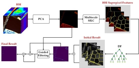
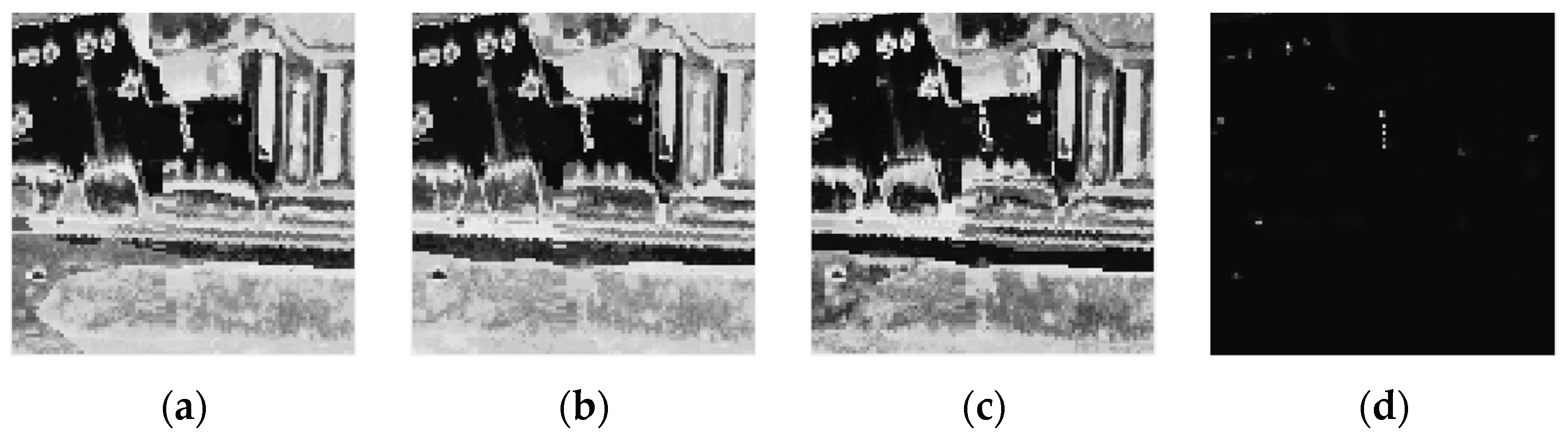
As displayed in Figure 4a–c, although the detection results of the DF can capture the anomaly pixels well on the Gainesville dataset, a large number of background pixels are erroneously detected as the abnormal, resulting in the high FARs. To this end, the module of multiscale fusion with guided filtering is proposed in this paper, which can integrate effectively the multiscale DF detection maps with different spatial information to generate the final detection result. The implementation process of MFGF is shown in Figure 5.
First, the multiscale results from the DFs are normalized, and they are fused by pixel-level multiplication to obtain the result R1. The fusion way can suppress the background, but a few anomaly pixels are missed. Then, the guided filtering [40] is applied to refine the details of the anomaly target, and it is defined as
where is a refined anomaly detection map, and the initial map of is R1; is a guide map, i.e., the top three principal components ; the and are linear coefficients, and they are defined as
where means the regularization parameters, and it is set to 0.001; and represent the mean matrix and covariance of guide image in the window centered at the pixel j, respectively; is an identity matrix; represents the number of pixels in the window ; denotes the refined anomaly detection map, i.e., R1; is the mean of a refined map in the window , and the size of the window is set to . More details are shown in [41,42]. Finally, the refined result Oi is combined with the initial fusion result of R1 by pixel-level addition to get the result of R2, and the final detection map R3 is obtained by pixel-level multiplication of R2 and Oi.
4. Experiment Results and Analysis
In this section, the experimental setup is introduced, and the qualitative and quantitative experiment comparisons are made to demonstrate the superiority of the proposed method. In addition, parameter analyses are carried out.
The experiments are implemented by a computer with Intel Core i7-9700 CPU at 3.00 GHz and 16 GB RAM (Intel, Santa Clara, CA, USA). The work platform of compared methods is MATLAB 2017b. The work platform of our method is python 3.6 with conda 4.5.4, and the applied packages are numpy 1.19.5, scipy 1.5.4, matplotlib 3.3.4, scikit-learn 0.24.2 and scikit-image 0.17.2.
4.1. Experiment Setup
4.1.1. Hyperspectral Dataset
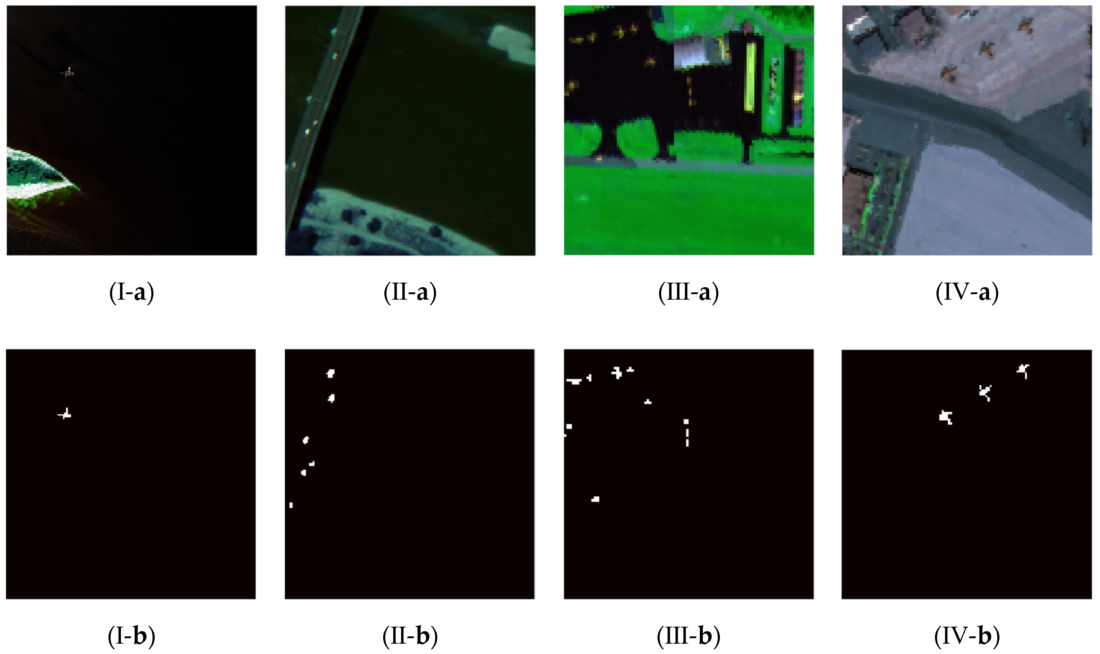
To effectively verify the performance of the proposed method, we conduct experiments on four public hyperspectral datasets, i.e., Cat Island, Pavia, Gainesville, and San Diego. More details are described in Table 1.
Cat Island Dataset: the first dataset, which is captured by the Airborne Visible/Infrared Imaging Spectrometer (AVIRIS) sensor on 12 September 2010. The dataset covers Gulfport, Southern Mississippi, USA. The size is 150 × 150 with 188 spectral bands, and the spatial resolution is 17.2 m/pixel. As shown in Figure 6(Ⅰ-a,Ⅰ-b), the anomaly object is an airplane with 19 pixels and accounts for 0.08% of the whole dataset.
Pavia Dataset: the second dataset is captured by the Reflective Optics System Imaging Spectrometer 03 (ROSIS-03) sensor, and its scene is the center of Pavia city in Northern Italy. The size is 150 × 150 with 102 spectral bands, and the spatial resolution is 1.3 m/pixel. The wavelength range is from 430 nm to 860 nm. Additionally, there are six anomaly targets in the dataset of Figure 6(Ⅱ-a,Ⅱ-b), and the number of anomaly pixels is 68 and 0.3% of the whole image.
Gainesville Dataset: the third dataset is captured by the AVIRIS sensor on 4 September 2010. The background is the city of Gainesville, FL, USA. The size of the dataset is 150 × 150, and the number of spectral bands is 102. The spatial resolution is 1.3 m/pixel. As is depicted in Figure 6(Ⅲ-a,Ⅲ-b), several buildings are anomaly objects, and it has 52 pixels and accounts for 0.52% of the whole dataset.
San Diego Dataset: the fourth dataset is captured by the AVRIS sensor, and the scene is the area of San Diego airport, CA, USA. The pixel size is 120 × 120, and the band number is 189. The spatial resolution is 3.5 m, and the range of wavelength is 400–2500 nm. Figure 6(Ⅳ-a,Ⅳ-b) are the pseudo color map and ground truth (GT), respectively. It is obvious that three airplanes are anomalies and have 57 pixels, which accounts for 0.4% of the total pixels of the dataset.
4.1.2. Compared Methods
The proposed algorithm is compared with six state-of-the-art algorithms in this paper, including RX [17], CRD [24], LRASR [9], LSDM-MoG [29], SSDF [15], and KIFD [13]. The RX is a classical statistics-based method. The CRD is a collaborative representation method. the LRASR and LSDM-MoG are low-rank representation methods. All settings of compared methods refer to the corresponding papers.
4.1.3. Evaluation Metrics
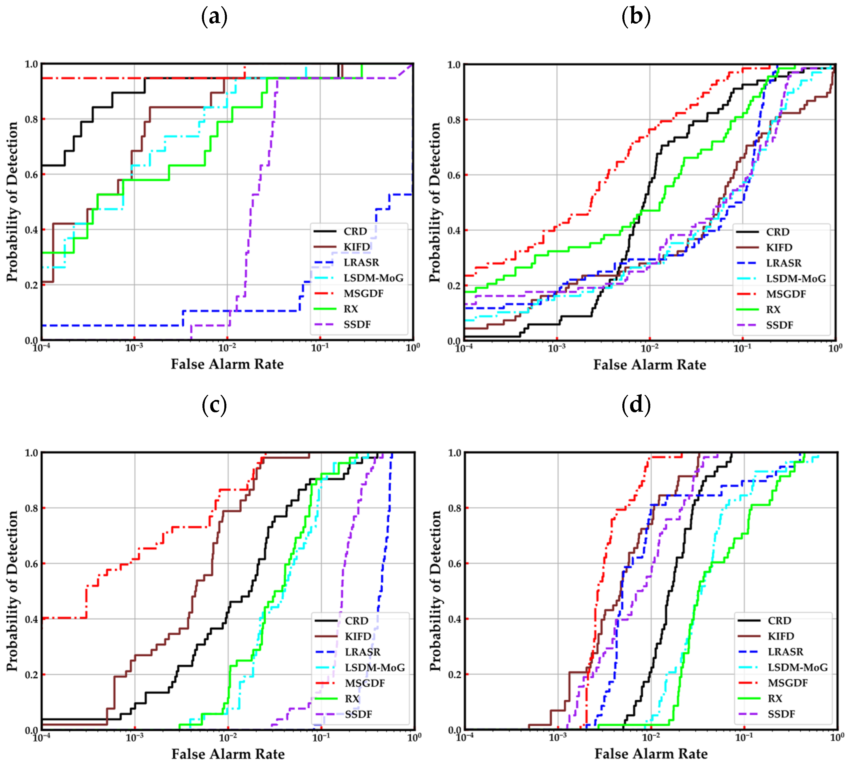
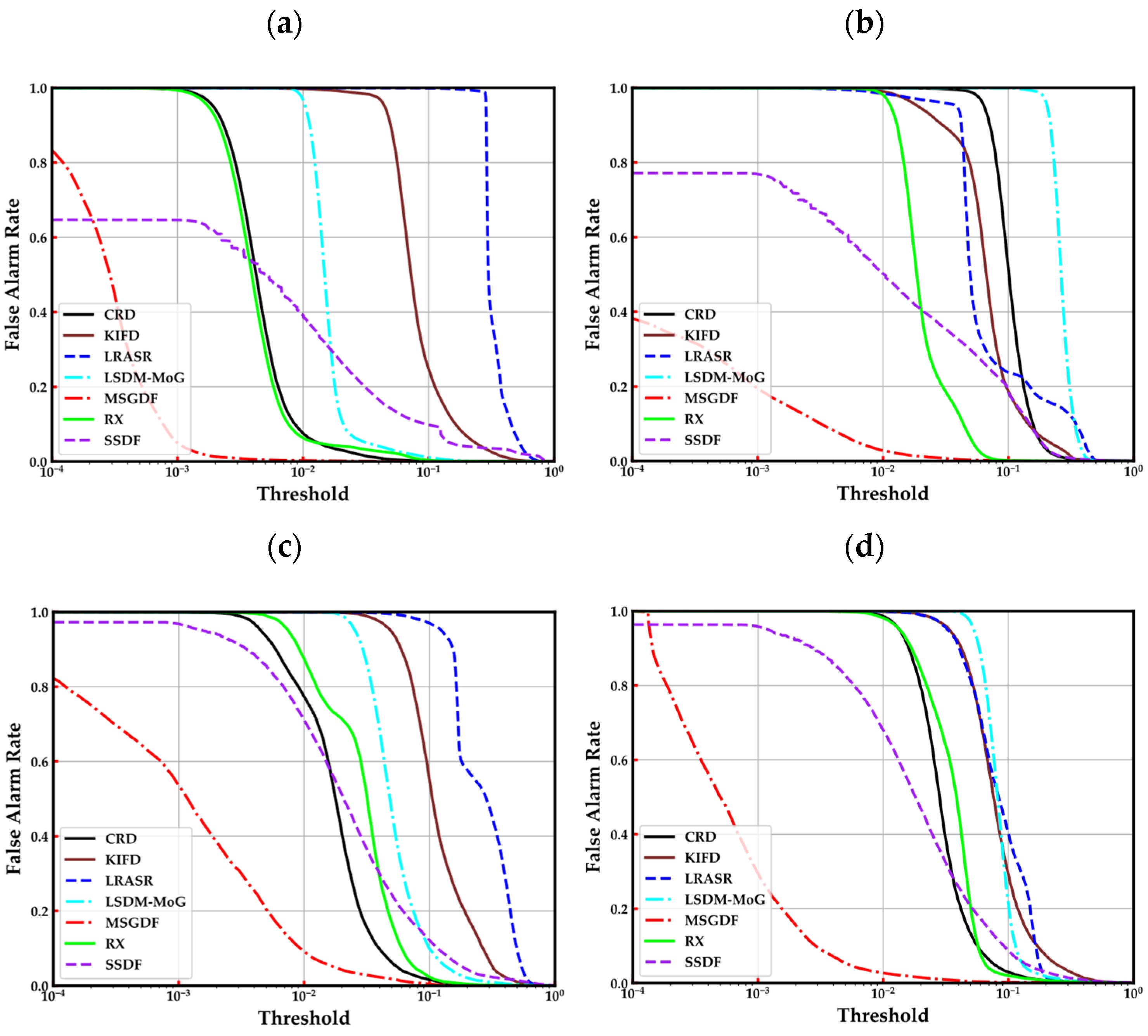
To effectively evaluate the performance of the proposed method, we apply four commonly used evaluation indicators, i.e., the area under the curve (AUC) of (Pd, Pf) and (Pf, τ), the receiver operating characteristic (ROC) curve of (Pd, Pf) and (Pf, τ), the time complexity and running time.
The ROC curve is to describe the tradeoff between the probability of detection (Pd) and the false alarm rate (Pf). When the threshold (τ) is set to an anomaly detection map, the probabilities of Pd and Pf can be obtained by the formula of
where denotes the total number of true target pixels in an HSI, and represents the number of true object pixels which are detected as objects; means the total number of background pixels in an HSI, and means denotes the total number of pixels in the HSI. By the effect of different threshold τ, the corresponding value of Pd and Pf can generate the ROC curve of (Pd, Pf) and (Pf, τ). Notably, the ROC curve of (Pd, Pf) is close to the upper left, and the performance is better; the ROC curve of (Pf, τ) is close to the lower left, and the detection effect is better.
The AUC, which is obtained by calculating the area of ROC, is applied to quantitatively evaluate the detection performance. Correspondingly, the value of AUC has (Pd, Pf) and (Pf, τ). When detection performance is better, the AUC of (Pd, Pf) is larger, and the AUC of (Pf, τ) is smaller.
In addition, the time complexity and running time are utilized to estimate the efficiency of different methods.
4.2. Detection Performance
In this section, the qualitative and quantitative comparisons are to evaluate the detection performance. For example, Figure 7 is the color detection map to make a quantitative comparison, and Table 2 and Table 3, Figure 8 and Figure 9 are the quantitative comparisons.
4.2.1. Qualitative Comparison
The qualitative comparison of detection color maps on four datasets is exhibited in Figure 7. Compared with other methods, the MSGDF method detects anomalous objects accurately and clearly in various complex backgrounds. For example, as for the Pavia detection maps of IF-based methods, the SSDF method cannot detect some anomaly objects of the buildings; in the KIFD method, although it can detect the buildings well, many background pixels are incorrectly detected; the proposed MSGDF method can detect all anomaly objects of buildings in the situation of low FARs. Hence, the proposed method has a better detection ability in subjective comparison.
Figure 7.
Color detection maps on four datasets.


4.2.2. Quantitative Comparison
The AUC comparisons are depicted in Table 2. From the AUC value in the single and entire dataset, the proposed MSGDF method has the best performance of the AUC of (Pd, Pf) and the AUC of (Pf, τ) in all methods. Meanwhile, compared with the algorithm of the second-best performance, the proposed algorithm has obvious advantages. Specifically, on the Cat Island dataset, the AUC score of (Pd, Pf) is 0.9992 and close to the ideal value of 1 in the proposed method, and our AUC score of (Pf, τ) is 0.0005 and close to 0, which is evidently superior to the CRD methods of the second-best performance. As for the challenging Pavia dataset, the RX has good detection performance, and its AUC value of (Pd, Pf) and (Pf, τ) are 0.9538 and 0.0233; in the proposed MSGDF method, our AUC value of (Pd, Pf) is 0.9868, which is 0.033 higher than the RX, and our AUC value of (Pf, τ) is 0.0014, which is 0.0216 lower than the RX. Furthermore, the AUC score of IF-based methods is listed in Table 2, we observe that the IF-based methods cannot acquire good performance of the AUC of (Pd, Pf) and (Pf, τ) at the same time. Taking the Gainesville dataset as an example, in the KIFD method, its AUC score of (Pd, Pf) and (Pf, τ) are 0.9921, and 0.1374, so we can think that the KIFD has a high AUC score of (Pd, Pf) and (Pd, Pf); on the contrary, the SSDF method has the low AUC score of (Pd, Pf) and (Pd, Pf), and its AUC score of (Pd, Pf) and (Pf, τ) are 0.8181 and 0.0506; in the proposed MSGDF method, it acquires a high AUC score of (Pd, Pf) and low AUC score of (Pd, Pf), the AUC score of (Pd, Pf) and (Pf, τ) are 0.9961 and 0.0047, respectively. In summary, the proposed method has a better detection rate and false alarm rate in the AUC comparison.

Table 2.
AUC of (Pd, Pf) and (Pf,τ) on the four datasets. The bold mark and underlined mark indicate the first- and second-best performance, respectively.
Table 2.
AUC of (Pd, Pf) and (Pf,τ) on the four datasets. The bold mark and underlined mark indicate the first- and second-best performance, respectively.
| Datasets | RX [17] | CRD [24] | LRASR [9] | LSDM-MoG [29] | SSDF [15] | KIFD [13] | MSGDF |
|---|---|---|---|---|---|---|---|
| AUC of (Pd, Pf) | |||||||
| Cat Island | 0.9807 | 0.9916 | 0.4203 | 0.9942 | 0.9368 | 0.9897 | 0.9992 |
| Pavia | 0.9538 | 0.9537 | 0.9146 | 0.8646 | 0.8856 | 0.8164 | 0.9868 |
| Gainesville | 0.9513 | 0.9597 | 0.5897 | 0.9438 | 0.8181 | 0.9921 | 0.9961 |
| San Diego | 0.9111 | 0.9791 | 0.9853 | 0.9320 | 0.9884 | 0.9922 | 0.9960 |
| Average value | 0.9492 | 0.9710 | 0.7275 | 0.9337 | 0.9072 | 0.9476 | 0.9945 |
| AUC of (Pf, τ) | |||||||
| Cat Island | 0.0065 | 0.0058 | 0.3398 | 0.0181 | 0.0417 | 0.0952 | 0.0005 |
| Pavia | 0.0233 | 0.1104 | 0.1073 | 0.2708 | 0.0462 | 0.0815 | 0.0014 |
| Gainesville | 0.0351 | 0.0229 | 0.2979 | 0.0619 | 0.0506 | 0.1374 | 0.0047 |
| San Diego | 0.0406 | 0.0360 | 0.0975 | 0.0882 | 0.0399 | 0.0980 | 0.0021 |
| Average value | 0.0264 | 0.0438 | 0.2106 | 0.1098 | 0.0446 | 0.1030 | 0.0022 |
The ROC curves of (Pd, Pf) and (Pf, τ) are described in Figure 8 and Figure 9. As for the ROC curves of (Pd, Pf), we can observe that the curve of the proposed MSGDF algorithm is always at the top left of six compared algorithms on Cat Island, Pavia, and Gainesville datasets. In the San Diego dataset, A small part on the left of our curve is below the curve of the KIFD and LRASR methods, and the rest part of our curve is above the compared methods. From the overall curve, our method is also at the top left of the other methods. Therefore, the ROC curves of (Pd, Pf) illustrate that the proposed MSGDF method is superior to the compared methods. In the dimension of the ROC curves of (Pf, τ), it is evident that the curve of the proposed MSGDF is at the bottom left of six state-of-the-art algorithms, which indicates that our method has a better performance on the false alarm rates.
These experiment results illustrate that the proposed method has preeminent detection accuracy and FARs, which demonstrates that the design of MSGDF can better dig out HSI spectral–spatial information to detect local anomalies and improve the problem of high FARs.
Figure 8.
ROC curves of (Pd, Pf) on the four datasets. (a) Cat Island, (b) Pavia, (c) Gainesville, (d) San Diego.
Figure 8.
ROC curves of (Pd, Pf) on the four datasets. (a) Cat Island, (b) Pavia, (c) Gainesville, (d) San Diego.

Figure 9.
ROC curves of (Pf, τ) on the four datasets. (a) Cat Island, (b) Pavia, (c) Gainesville, (d) San Diego.
Figure 9.
ROC curves of (Pf, τ) on the four datasets. (a) Cat Island, (b) Pavia, (c) Gainesville, (d) San Diego.

The time complexity analysis of the proposed DF model is carried out, and the proposed DF model mainly consists of three parts, i.e., calculating the hyperplane projection value, computing the gain splitting criterion, and partitioning the projection attribute value. Therefore, the time complexity is O(tn(qn + logn + n)) in the training stage, and the time complexity of the evaluation stage is O(tnqN). The total time complexity of the proposed DF model is O(tn(q(n + N) + logn + n)). In addition, the comparison results of the running time on four HSI datasets are listed in Table 3, and it can be observed that the proposed MSGDF method is superior to the other methods, except the RX method. In the comparison of the IF-based methods, our method is the fastest. This is because the overall design of the proposed MSGDF model is relatively simple and valid to reduce time consumption. Two other IF-based methods are relatively complex, causing increasing the running time. Concretely, the KIFD algorithm adopts the kernel space and the iteration strategy to optimize its detector; the SSDF algorithm applies the axis-parallel subspace selection process and complex splitting criterion to enhance the discriminant ability. The strategies of KIFD and SSDF methods trade the lower running efficiency for high detection accuracy.
Table 3.
Running time on the four datasets. The bold mark and underlined mark indicate the first- and second-best performance, respectively.
Table 3.
Running time on the four datasets. The bold mark and underlined mark indicate the first- and second-best performance, respectively.
| Datasets | RX | CRD | LRASR | LSDM-MoG | SSDF | KIFD | MSGDF |
|---|---|---|---|---|---|---|---|
| Cat Island | 0.9065 | 16.4834 | 2.9095 | 47.4954 | 47.4678 | 71.2541 | 15.3171 |
| Pavia | 0.1729 | 14.7069 | 92.2870 | 20.2075 | 58.2189 | 87.1228 | 14.0285 |
| Gainesville | 0.4846 | 3.1657 | 1.5270 | 19.9304 | 40.4361 | 64.1250 | 3.3587 |
| San Diego | 0.5166 | 15.0573 | 1.8886 | 13.0941 | 47.2768 | 68.3000 | 6.3185 |
| Average value | 0.52015 | 12.35333 | 24.65303 | 25.18185 | 48.3499 | 72.70048 | 9.7557 |
4.3. Parameter Analysis
4.3.1. Parameter Analysis of Multiscale Superpixel Segmentation
The parameter setting in the number of superpixels is crucial for the HAD because it determines the feature extraction of HSI spatial information. In the article, the number of superpixels is set from 1 to 19, and the reason is that the range not only effectively distinguishes different types of homogeneous scene regions but also ensures the subsample number of each DF [14]. For the number of superpixel scale, its range is from 2 to 6, because this range can significantly reduce the false alarm rate in this paper. Moreover, to obtain the setting of multiscale superpixel segmentation, the single scale superpixel setting is acquired by selecting the best detection performance, and then based on the single scale superpixel setting, the number of multiscale superpixels is obtained by the best detection performance.
The AUC score of (Pd, Pf) of the single-scale superpixel DF is displayed in Figure 10. It can be observed that the superpixel-guided DF in the situation that the number of superpixels is over 1 is better than the original DF in the situation that the number of superpixels is 1 in the overall detection effect. Especially, when the optimum number of superpixels is selected, the advantage of single-scale superpixel DF is more obvious. This experiment results verify the necessity of the superpixel-guided DF in HAD. According to the best detection accuracy of (Pd, Pf) on four HSI datasets, the number of superpixels on Cat Island, Pavia, Gainesville, Los Angeles, and San Diego datasets are set to 17, 3, 9, and 5, respectively. Furthermore, we find that the best number setting of single-scale superpixels on each HSI data set is affected by the HSI scene complexity.
To facilitate the setting of multiscale superpixels on four HSI datasets, the superpixel number of the obtained single-scale setting is the center, which can set the other numbers of the multiscale superpixels. For the superpixel setting of every scale, we select the best detection accuracy in the superpixel number combination as the scale setting result. On the basis of the principles, the AUC scores of the multiscale superpixel setting (MSS) are listed in Table 4. From the AUC value of (Pf, τ), we can find that the false alarm rate decreases with the increase of the superpixel scales, and the best performance of FARs is got in the scale setting of 6. In the AUC score of (Pd, Pf), the detection accuracy of superpixel scale 3 is higher than the other scale. Finally, by considering comprehensively the AUC scores of (Pd, Pf) and (Pf, τ), when the number of the superpixel scale is 3, it can acquire the best performance of detection rates in the situation of low FARs. Therefore, the number settings of multiscale superpixels on the Cat Island, Pavia, Gainesville, Los Angeles, and San Diego datasets are set to (15, 17, 19), (1, 3, 5), (9, 11, 13), and (3, 5, 7), respectively.
4.3.2. Parameter Analysis of Discrimination Forest
The effect of three parameter settings in DF is analyzed in Figure 11, including the dimension (q), subsampling size (n), and the number of trees (t). To display clearly the impact of parameters, the red curve of average value is to represent the holistic detection impact, and the curve of other colors is to depict the changing trend in a single dataset. Significantly, the larger the value of the three parameters are, the more running time will be consumed.
Figure 11a depicts the influence of the subsample size n on AUC of (Pd, Pf), and the subsample setting range of DF is from 3% to 50% in each superpixel block. The AUC (Pd, Pf) value on the Cat Island dataset remains around 0.99; regarding the other three datasets, the AUC value begins to rise, then decreases, and finally tends to remain unchanged. Most notably, when the subsample is about 10–20%, the best performance of AUC (Pd, Pf) is gained on four datasets.
The number of dimensions q for the hyperplane building of DF is from 1 to 100. As is depicted in Figure 11b, the AUC values of (Pd, Pf) initially increase and then fluctuate in a small range on the four datasets, and the max AUC value of (Pd, Pf) is achieved at dimension number of 2. Furthermore, the changing trend of AUC curves illustrates that utilizing multi-dimension spectral bands is better than using a single-dimension spectral band in the DF. This phenomenon demonstrates the effectiveness of multi-dimension design on the gain split criterion.
The value of the number of discriminative trees is from 10 to 500 in Figure 11c. We observe that the changing trend of the AUC value of (Pd, Pf) is similar to Figure 11b, and the difference is that the AUC value of the Cat Island dataset changes slightly at 0.999.
Finally, according to comprehensive consideration of the average detection accuracy and time consumption, the parameters of dimension and trees are set to 2 and 100 respectively, and the subsample size is 10% of pixels in each HSI superpixel block.
5. Discussion
To illustrate the effectiveness of DF, the IF and proposed DF are tested on four HSI datasets, and their results with the AUC of (Pd, Pf) are displayed in Figure 12. From the detection accuracy results, the proposed DF is superior to the original IF both in the AUC (Pd, Pf) of the single dataset and average AUC (Pd, Pf) of the entire dataset, and the average AUC value of the DF method is 2% higher than the average AUC value of IF method. This verifies that the design of the DF is more sensitive to anomaly pixels than the design of the original IF. Meanwhile, it illustrates that the strategy of the gain split criterion and acceptable range is effective in the DF model.
To further explain the influence of improved strategies in our proposed DF, such as the gain split criterion and acceptable range, the experiment of component analysis is conducted in four hyperspectral data sets, and the results of detection accuracy are listed in Table 5. Under the strategy of gain split criterion or acceptable range, the average AUC score of (Pd, Pf) of improved DF is over 1% higher than without improved DF, meanwhile, the AUC score rises up on each hyperspectral data set. These results illustrate the efficiency of two design strategies. On the other side, compared with adopting a single optimization strategy, the way of gain split criterion combined with acceptable range further improves AUC accuracy in each data set and the entire data sets, which verifies the rationality of combination of two optimization strategies.
6. Conclusions
A novel detection strategy with the MSGDF model is proposed for HAD. In this model, the multiscale superpixel segmentation is applied to excavate spatial features and guide local anomaly detection, and the split criterion of multi-dimension spectral bands is adopted to optimize each node division for the DF. The strategy, which combines DF with SLIC, makes full use of HSI spectral and spatial information to solve the problem of local anomalies. In addition, the MFGF is put forward to effectively reduce FARs of initial DF results. Finally, the experimental analysis validates the rationality of the MSGDF method, and the detection results illustrate that the MSGDF has better detection ability than state-of-the-art algorithms. Although the performance of our proposed algorithm is satisfactory, some meaningful problems remain to be explored in our future work. Specifically, the obtained background pixels are constructed semi-supervised iforest to enhance the sensitivity of anomalies in test stage. Furthermore, whether the IF methods can combine with the other HAD methods to improve detection effect, such as LRR, CR and AE.
Author Contributions
X.C., H.W. and M.Z. provide the methodology and Conceptualization; X.C. write original draft; X.C., S.L., K.Z. and L.W. implement experiments; S.L., K.Z., H.W. and M.Z. revise the manuscript. All authors have read and agreed to the published version of the manuscript.
Funding
This research was funded by the National Natural Science Foundation of China (No. 12003018), Fundamental Research Funds for the Central Universities (No. XJS191305), and China Postdoctoral Science Foundation (No. 2018M633471).
Data Availability Statement
The hyperspectral data in this paper are available at http://xudongkang.weebly.com/ (accessed on 10 January 2021).
Acknowledgments
The authors gratefully acknowledge the School of Aerospace Science and Technology, Xidian University. Meanwhile, we thank those researchers who have provided open-source codes and data in the area of hyperspectral anomaly detection.
Conflicts of Interest
The authors declare no conflict of interest.
Abbreviations and Acronyms
| HSI | hyperspectral image |
| HAD | hyperspectral anomaly detection |
| IF | isolation forest |
| KIFD | kernel isolation forest detection |
| KPCA | kernel principal component analysis |
| MFIFD | isolation forest method based on multiple features |
| EMP | extend morphological profile |
| EMAP | extend multi-attribute profile |
| SSDF | subspace selection-based discriminative forest |
| DF | discriminative forest |
| MFGF | multiscale fusion with guided filtering |
| FAR | false alarm rate |
| MSGDF | multiscale superpixel guided discriminative forest |
| RX | Reed-Xiaoli |
| CR | collaborative representation |
| LRR | low-rank representation |
| LRASR | low-rank and sparse representation |
| LSDM-MoG | low-rank and sparse decomposition model with the mixture of the gaussian model |
| GAN | generative adversarial network |
| AE | autoencoder |
| AEAN | autoencoder adversarial network |
| SLIC | simple linear iterative clustering |
| PCA | principal component analysis |
| SSIIF | spectral-spatial anomaly detector based on improved Isolation Forest |
| AVIRIS | Airborne Visible/Infrared Imaging Spectrometer |
| ROSIS-03 | Reflective Optics System Imaging Spectrometer 03 |
| GT | ground truth |
| AUC | area under the curve |
| ROC | receiver operating characteristic |
| MSS | multiscale superpixel setting |
References
- Qi, J.; Gong, Z.; Yao, A.; Liu, X.; Li, Y.; Zhang, Y.; Zhong, P. Bathymetric-based band selection method for hyperspectral underwater target detection. Remote Sens. 2021, 13, 3798. [Google Scholar] [CrossRef]
- Dong, Y.; Shi, W.; Du, B.; Hu, X.; Zhang, L. Asymmetric weighted logistic metric learning for hyperspectral target detection. IEEE Trans Cybern. 2021, 52, 11093–11106. [Google Scholar] [CrossRef] [PubMed]
- Cheng, X.; Wen, M.; Gao, C.; Wang, Y. Hyperspectral anomaly detection based on wasserstein distance and spatial filtering. Remote Sens. 2022, 14, 2730. [Google Scholar] [CrossRef]
- Huang, J.; Liu, K.; Li, X. Locality constrained low rank representation and automatic dictionary learning for hyperspectral anomaly detection. Remote Sens. 2022, 14, 1327. [Google Scholar] [CrossRef]
- Han, X.; Jiang, Z.; Liu, Y.; Zhao, J.; Sun, Q.; Li, Y. A spatial–spectral combination method for hyperspectral band selection. Remote Sens. 2022, 14, 3217. [Google Scholar] [CrossRef]
- Wang, Q.; Zhang, F.; Li, X. Optimal clustering framework for hyperspectral band selection. IEEE Trans. Geosci. Remote Sens. 2018, 56, 5910–5922. [Google Scholar] [CrossRef]
- Rebeyrol, S.; Deville, Y.; Achard, V.; Briottet, X.; May, S. Using a panchromatic image to improve hyperspectral unmixing. Remote Sens. 2020, 12, 2834. [Google Scholar] [CrossRef]
- Rasti, B.; Koirala, B.; Scheunders, P.; Ghamisi, P. How hyperspectral image unmixing and denoising can boost each other. Remote Sens. 2020, 12, 1728. [Google Scholar] [CrossRef]
- Xu, Y.; Wu, Z.; Li, J.; Plaza, A.; Wei, Z. Anomaly detection in hyperspectral images based on low-rank and sparse representation. IEEE Trans. Geosci. Remote Sens. 2016, 54, 1990–2000. [Google Scholar] [CrossRef]
- Su, H.; Wu, Z.; Zhang, H.; Du, Q. Hyperspectral anomaly detection: A survey. IEEE Geosci Remote Sens Mag. 2022, 10, 64–90. [Google Scholar] [CrossRef]
- Xu, Y.; Zhang, L.; Du, B.; Zhang, L. Hyperspectral anomaly detection based on machine learning: An overview. IEEE J. Sel. Top. Appl. Earth Obs. Remote Sens. 2022, 15, 3351–3364. [Google Scholar] [CrossRef]
- Liu, F.T.; Ting, K.M.; Zhou, Z.H. Isolation forest. In Proceedings of the 2008 Eighth IEEE International Conference on Data Mining, Pisa, Italy, 15–19 December 2008; pp. 413–422. [Google Scholar]
- Li, S.; Zhang, K.; Duan, P.; Kang, X. Hyperspectral anomaly detection with kernel isolation forest. IEEE Trans. Geosci. Remote Sens. 2020, 58, 319–329. [Google Scholar] [CrossRef]
- Wang, R.; Nie, F.; Wang, Z.; He, F.; Li, X. Multiple features and isolation forest-based fast anomaly detector for hyperspectral imagery. IEEE Trans. Geosci. Remote Sens. 2020, 58, 6664–6676. [Google Scholar] [CrossRef]
- Chang, S.; Du, B.; Zhang, L. A subspace selection-based discriminative forest method for hyperspectral anomaly detection. IEEE Trans. Geosci. Remote Sens. 2020, 58, 4033–4046. [Google Scholar] [CrossRef]
- Song, X.; Aryal, S.; Ting, K.M.; Liu, Z.; He, B. Spectral–spatial anomaly detection of hyperspectral data based on improved isolation forest. IEEE Trans. Geosci. Remote Sens. 2021, 60, 5516016. [Google Scholar] [CrossRef]
- Reed, I.S.; Yu, X. Adaptive multiple-band CFAR detection of an optical pattern with unknown spectral distribution. IEEE Trans. Acoust. Speech Signal Process. 1990, 38, 1760–1770. [Google Scholar] [CrossRef]
- Heesung, K.; Nasrabadi, N.M. Kernel RX-algorithm: A nonlinear anomaly detector for hyperspectral imagery. IEEE Trans. Geosci. Remote Sens. 2005, 43, 388–397. [Google Scholar] [CrossRef]
- Molero, J.M.; Garzon, E.M.; Garcia, I.; Plaza, A. Analysis and optimizations of global and local versions of the RX algorithm for anomaly detection in hyperspectral data. IEEE J. Sel. Topics Appl. Earth Observ. Remote Sens. 2013, 6, 801–814. [Google Scholar] [CrossRef]
- Guo, Q.; Zhang, B.; Ran, Q.; Gao, L.; Li, J.; Plaza, A. Weighted-RXD and linear filter-based RXD: Improving background statistics estimation for anomaly detection in hyperspectral imagery. IEEE J. Sel. Top. Appl. Earth Obs. Remote Sens. 2014, 7, 2351–2366. [Google Scholar] [CrossRef]
- Tao, R.; Zhao, X.; Li, W.; Li, H.; Du, Q. Hyperspectral anomaly detection by fractional Fourier entropy. IEEE J. Sel. Top. Appl. Earth Obs. Remote Sens. 2019, 12, 4920–4929. [Google Scholar] [CrossRef]
- Yuan, S.R.; Shi, L.; Yao, B.; Li, F.Y.; Du, Y.F. A hyperspectral anomaly detection algorithm Using sub-features grouping and binary accumulation. IEEE Geosci. Remote Sens. Lett. 2022, 19, 6007505. [Google Scholar] [CrossRef]
- Cheng, T.; Wang, B. Graph and total variation regularized low-rank representation for hyperspectral anomaly detection. IEEE Trans. Geosci. Remote Sens. 2019, 58, 391–406. [Google Scholar] [CrossRef]
- Li, W.; Du, Q. Collaborative representation for hyperspectral anomaly detection. IEEE Trans. Geosci. Remote Sens. 2015, 53, 1463–1474. [Google Scholar] [CrossRef]
- Tu, B.; Li, N.; Liao, Z.; Ou, X.; Zhang, G. Hyperspectral anomaly detection via spatial density background purification. Remote Sens. 2019, 11, 2618. [Google Scholar] [CrossRef]
- Lin, S.; Zhang, M.; Cheng, X.; Wang, L.; Xu, M.; Wang, H. Hyperspectral anomaly detection via dual dictionaries construction guided by two-stage complementary decision. Remote Sens. 2022, 14, 1784. [Google Scholar] [CrossRef]
- Jiang, K.; Xie, W.; Li, Y.; Lei, J.; He, G.; Du, Q. Semisupervised spectral learning with generative adversarial network for hyperspectral anomaly detection. IEEE Trans. Geosci. Remote Sens. 2020, 58, 5224–5236. [Google Scholar] [CrossRef]
- Arisoy, S.; Nasrabadi, N.M.; Kayabol, K. Unsupervised pixel-wise hyperspectral anomaly detection via autoencoding adversarial Networks. IEEE Geosci. Remote Sens. Lett. 2021, 19, 5502905. [Google Scholar] [CrossRef]
- Lu, L.; Wei, L.; Qian, D.; Ran, T. Low-rank and sparse decomposition with mixture of Gaussian for hyperspectral anomaly detection. IEEE Trans Cybern. 2020, 51, 4363–4372. [Google Scholar]
- Qian, X.; Lin, S.; Cheng, G.; Yao, X.; Ren, H.; Wang, W. Object detection in remote sensing images based on improved bounding box regression and multi-level features fusion. Remote Sens. 2020, 12, 143. [Google Scholar] [CrossRef]
- Zhou, K.; Zhang, M.; Wang, H.; Tan, J. Ship detection in SAR images based on multi-scale feature extraction and adaptive feature fusion. Remote Sens. 2022, 14, 755. [Google Scholar] [CrossRef]
- Qian, X.; Cheng, X.; Cheng, G.; Yao, X.; Jiang, L. Two-stream encoder GAN with progressive training for co-saliency detection. IEEE Signal Process Lett. 2021, 28, 180–184. [Google Scholar] [CrossRef]
- Achanta, R.; Shaji, A.; Smith, K.; Lucchi, A.; Fua, P.; Süsstrunk, S. SLIC Superpixels compared to state-of-the-art superpixel methods. IEEE Trans. Pattern Anal. Mach. Intell. 2012, 34, 2274–2282. [Google Scholar] [CrossRef] [PubMed]
- Huang, Z.; Fang, L.; Li, S. Subpixel-pixel-superpixel guided fusion for hyperspectral anomaly detection. IEEE Trans. Geosci. Remote Sens. 2020, 58, 5998–6007. [Google Scholar] [CrossRef]
- Ren, L.; Zhao, L.; Wang, Y. A superpixel-based dual window RX for hyperspectral anomaly detection. IEEE Geosci. Remote Sens. Lett. 2020, 17, 1233–1237. [Google Scholar] [CrossRef]
- Feng, R.; Li, H.; Wang, L.; Zhong, Y.; Zhang, L.; Zeng, T. Local spatial constraint and total variation for hyperspectral anomaly detection. IEEE Trans. Geosci. Remote Sens. 2022, 60, 5512216. [Google Scholar] [CrossRef]
- Abdi, H.; Williams, L.J. Principal component analysis. Comput. Stat. 2010, 2, 433–459. [Google Scholar] [CrossRef]
- Cortes, D. Revisiting randomized choices in isolation forests. arXiv 2021, arXiv:2110.13402. [Google Scholar]
- Liu, F.T.; Ting, K.M.; Zhou, Z.-H. On detecting clustered anomalies using SCiForest. In Proceedings of the ECML-PKDD, Barcelona, ES, USA, 20–24 September 2010; pp. 274–290. [Google Scholar]
- He, K.; Sun, J.; Tang, X. Guided image filtering. IEEE Trans. Pattern Anal. Mach. Intell. 2012, 35, 1397–1409. [Google Scholar] [CrossRef]
- Xie, W.; Jiang, T.; Li, Y.; Jia, X.; Lei, J. Structure tensor and guided filtering-based algorithm for hyperspectral anomaly detection. IEEE Trans. Geosci. Remote Sens. 2019, 57, 4218–4230. [Google Scholar] [CrossRef]
- Kang, X.; Zhang, X.; Li, S.; Li, K.; Li, J.; Benediktsson, J.A. Hyperspectral anomaly detection with attribute and edge-preserving filters. IEEE Trans. Geosci. Remote Sens. 2017, 55, 5600–5611. [Google Scholar] [CrossRef]
Figure 1.
The detection maps of isolation forest methods on the Gainesville dataset. (a) Pseudo color maps, (b) ground truth, (c,d) are the detection maps of existing IF-based methods, (e) the detection map of proposed MSGDF method.
Figure 1.
The detection maps of isolation forest methods on the Gainesville dataset. (a) Pseudo color maps, (b) ground truth, (c,d) are the detection maps of existing IF-based methods, (e) the detection map of proposed MSGDF method.

Figure 2.
Framework of the proposed MSGDF method. First, The PCA and SLIC module are applied to obtain multiscale HSI superpixel features with homogeneous information; then, each block in a HSI superpixel feature conducts the DF training and testing separately to generate the initial result; finally, the initial results are refined to obtain the final result by the MFGF module.

Figure 3.
Acceptable range of z in each sub-node. S denotes best split threshold, and v means the difference between the maximum and minimum of z.
Figure 3.
Acceptable range of z in each sub-node. S denotes best split threshold, and v means the difference between the maximum and minimum of z.

Figure 4.
Initial detection maps of DF on the Gainesville dataset. (a–c) Are initial detection maps with different numbers of superpixels, and (d) is the ground truth.
Figure 4.
Initial detection maps of DF on the Gainesville dataset. (a–c) Are initial detection maps with different numbers of superpixels, and (d) is the ground truth.

Figure 5.
Flowchart of the proposed MFGF module.

Figure 6.
Descriptions of the experimental datasets. (a) pseudo color maps, (b) ground truth. (Ⅰ) Cat Island, (Ⅱ) Pavia, (Ⅲ) Gainesville, and (Ⅳ) San Diego.
Figure 6.
Descriptions of the experimental datasets. (a) pseudo color maps, (b) ground truth. (Ⅰ) Cat Island, (Ⅱ) Pavia, (Ⅲ) Gainesville, and (Ⅳ) San Diego.

Figure 10.
Number of superpixels for the influence of (Pd, Pf) AUC in DF.

Figure 11.
Effect of three parameter settings in proposed MSGDF model. (a) Subsample size, (b) Dimensions and (c) Number of trees.
Figure 11.
Effect of three parameter settings in proposed MSGDF model. (a) Subsample size, (b) Dimensions and (c) Number of trees.


Figure 12.
AUC comparison of (Pd, Pf) between IF and DF.

Table 1.
Details of the Cat Island, Pavia, Gainesville, and San Diego datasets.
| Dataset | Sensor | Spatial Resolution | Image Size | Anomaly Types |
|---|---|---|---|---|
| Cat Island | AVRIS | 17.2 m/pixel | 150 × 150 × 188 | Airplanes |
| Pavia | ROSIS-03 | 1.3 m/pixel | 150 × 150 × 102 | Vehicles |
| Gainesville | AVRIS | 3.5 m/pixel | 100 × 100 × 191 | Buildings |
| San Diego | AVRIS | 3.5 m/pixel | 120 × 120 × 189 | Airplanes |
Table 4.
Number of superpixel scales for the influence of AUC in MSGDF. The bold mark indicates the best performance.
Table 4.
Number of superpixel scales for the influence of AUC in MSGDF. The bold mark indicates the best performance.
| Scale | 2 | 3 | 4 | 5 | 6 | |
|---|---|---|---|---|---|---|
| MSS | (15, 17) | (15, 17, 19) | (13–19) | (11–19) | (9–19) | |
| Cat Island | AUC of (Pd, Pf) | 0.9976 | 0.9992 | 0.9990 | 0.9990 | 0.9992 |
| AUC of (Pf, τ) | 0.0033 | 0.0005 | 0.0001 | 0.0001 | 0 | |
| MSS | (3, 5) | (1, 3, 5) | (7–13) | (7–15) | (7–17) | |
| Pavia | AUC of (Pd, Pf) | 0.9807 | 0.9961 | 0.9958 | 0.9959 | 0.996 |
| AUC of (Pf, τ) | 0.0065 | 0.0047 | 0.0041 | 0.0016 | 0.001 | |
| MSS | (9, 11) | (9, 11, 13) | (7–13) | (7–15) | (7–17) | |
| Gainesville | AUC of (Pd, Pf) | 0.9940 | 0.9961 | 0.9958 | 0.9959 | 0.996 |
| AUC of (Pf, τ) | 0.0224 | 0.0047 | 0.0041 | 0.0016 | 0.001 | |
| MSS | (5, 7) | (3, 5, 7) | (1–7) | (1–9) | (1–11) | |
| San Diego | AUC of (Pd, Pf) | 0.9948 | 0.996 | 0.9948 | 0.9946 | 0.9942 |
| AUC of (Pf, τ) | 0.0087 | 0.0021 | 0.0024 | 0.0008 | 0.0004 | |
| Average Value | AUC of (Pd, Pf) | 0.9918 | 0.9945 | 0.9930 | 0.9929 | 0.9930 |
| AUC of (Pf, τ) | 0.0102 | 0.0022 | 0.0018 | 0.0007 | 0.0004 | |
Table 5.
The proposed DF component analysis by AUC of (Pd, Pf).
| Optimization Strategies | Hyperspectral Data Set | Average | ||||
|---|---|---|---|---|---|---|
| Gain Split Criterion | Acceptable Range | Cat Island | Pavia | Gainesville | San Diego | |
| 0.9685 | 0.9409 | 0.9596 | 0.9747 | 0.9609 | ||
| √ | 0.9800 | 0.9668 | 0.9680 | 0.9798 | 0.9737 | |
| √ | 0.9837 | 0.9608 | 0.9610 | 0.9821 | 0.9719 | |
| √ | √ | 0.9855 | 0.9760 | 0.9773 | 0.9832 | 0.9805 |
Publisher’s Note: MDPI stays neutral with regard to jurisdictional claims in published maps and institutional affiliations. |
© 2022 by the authors. Licensee MDPI, Basel, Switzerland. This article is an open access article distributed under the terms and conditions of the Creative Commons Attribution (CC BY) license (https://creativecommons.org/licenses/by/4.0/).
Share and Cite
MDPI and ACS Style
Cheng, X.; Zhang, M.; Lin, S.; Zhou, K.; Wang, L.; Wang, H. Multiscale Superpixel Guided Discriminative Forest for Hyperspectral Anomaly Detection. Remote Sens. 2022, 14, 4828. https://0-doi-org.brum.beds.ac.uk/10.3390/rs14194828
AMA Style
Cheng X, Zhang M, Lin S, Zhou K, Wang L, Wang H. Multiscale Superpixel Guided Discriminative Forest for Hyperspectral Anomaly Detection. Remote Sensing. 2022; 14(19):4828. https://0-doi-org.brum.beds.ac.uk/10.3390/rs14194828
Chicago/Turabian StyleCheng, Xi, Min Zhang, Sheng Lin, Kexue Zhou, Liang Wang, and Hai Wang. 2022. "Multiscale Superpixel Guided Discriminative Forest for Hyperspectral Anomaly Detection" Remote Sensing 14, no. 19: 4828. https://0-doi-org.brum.beds.ac.uk/10.3390/rs14194828
Note that from the first issue of 2016, this journal uses article numbers instead of page numbers. See further details here.