Article

Source-Independent Waveform Inversion Method for Ground Penetrating Radar Based on Envelope Objective Function

1
School of Geomatics and Prospecting Engineering, Jilin Jianzhu University, Changchun 130026, China
2
Science and Technology on Near-Surface Detection Laboratory, Wuxi 214035, China
3
College of Geo-Exploration Science and Technology, Jilin University, Changchun 130026, China
4
School of Civil Engineering, Guangzhou University, Guangzhou 510000, China
*
Author to whom correspondence should be addressed.
Remote Sens. 2022, 14(19), 4878; https://0-doi-org.brum.beds.ac.uk/10.3390/rs14194878
Submission received: 26 July 2022 / Revised: 22 September 2022 / Accepted: 26 September 2022 / Published: 29 September 2022
(This article belongs to the Special Issue Latest Results on GPR Algorithms, Applications and Systems)

Abstract

:
For the full waveform inversion, it is necessary to provide an accurate source wavelet for forwarding modeling in the iteration. The source wavelet estimation method based on deconvolution technology can solve this problem to some extent, but we find that the estimated source wavelet is not accurate and needs to be manually corrected repeatedly in the iteration. This process is highly operator-intensive, and the update process is time-consuming and increases the potential for errors. We propose a source-independent waveform inversion (SIEWI) scheme for cross-hole GPR data, and use the envelope objective function combined with this method to effectively reduce the nonlinearity of inversion. The residual field used by SIEWI to construct the gradient inherits the characteristics of the envelope wavefield. Compared with full waveform inversion (FWI), SIEWI is more robust and less sensitive to frequency components and inaccurate source wavelet. To avoid cycle jumping, the multi-scale strategy effectively utilizes the properties of convolutional wavefields. In one iteration, the wavefield is decomposed into multiple frequency bands through multiple convolutions in the time domain to construct a multi-scale inversion strategy that preferentially inverts low-frequency information.

1. Introduction

Ground penetrating radar (GPR) is widely used in archaeological, environmental, hydrological and engineering surveys to detect subsurface structures [1,2,3]. The most widely used GPR detection method is a non-destructive survey method in which the transmitters and receivers are placed on the ground at the same time. This paper focuses on the cross-hole GPR method (typically 20–250 MHz), where the transmitters and receivers are placed in two nearby boreholes, respectively. High-resolution tomographic images of the permittivity and conductivity between the two boreholes are provided by inversion of the direct wave information propagating in the interval between the two boreholes. The vertical depth of this detection method depends on the depth of the borehole, and it can penetrate the regolith to detect the deep formation. Its lateral detection range can be greater than 100 m in crystalline rocks, while in relatively conductive rocks (200–300 Ω·m), the detection range can reach 10–20 m. In addition to the detection range, the radar can perform multiple repeated detections at key locations, using stack averaging to improve the signal-to-noise ratio.
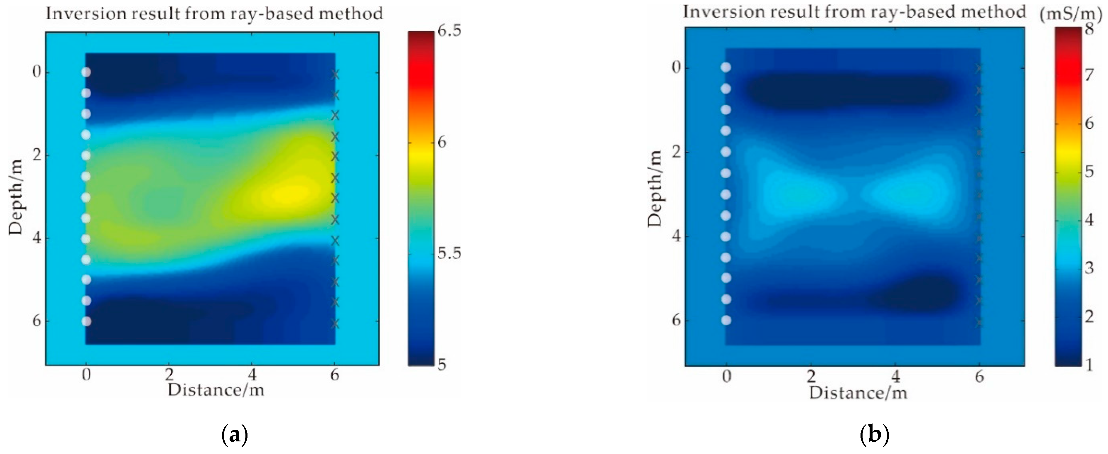
Traditional cross-hole GPR tomography methods are generally based on ray theory, such as the ray tracing method based on the first-arrival traveltime [4,5,6,7,8] and the attenuation tomography based on the maximum amplitude (centroid frequency downshift method) [9], which can invert the permittivity and conductivity, respectively. The traveltime tomographic inversion method is theoretically more mature and can provide reliable velocity inversion results. However, attenuation imaging is still theoretically inadequate and can only reflect the relative conductivity distribution between the target body and the formation. In addition, the tomographic inversion method based on ray theory utilizes part of the signal information, so that the tomographic method can only image anomalies larger than the dominant wavelength of the signal. The resolution is around the width of the first Fresnel zone [10,11]. Waveform inversion can utilize complete waveform information. Under the most ideal conditions, its resolution can reach the sub-wavelength level [12,13] (one-half to one-third wavelength).
The full waveform inversion method has achieved a series of achievements in the field of seismic first, and then gradually developed in the field of ground penetrating radar. In terms of seismic, Tarantola et al. [14,15,16] proposed a time-domain full waveform inversion based on generalized least squares inversion theory. The gradient direction is constructed by using the cross-correlation of the forward wavefield and the residual backpropagation wavefield, thus avoiding the direct calculation of the Fréchet derivative. Subsequently, Pratt et al. [17,18] extended it to the frequency domain and formed the frequency domain waveform inversion to improve the computational efficiency. For GPR, Kuroda et al. [19] and Meles et al. [20] used the GPR full waveform inversion method, which is similar to the seismic waveform inversion method, to image the cross-hole GPR data and achieved good results. Kuroda et al. only considered the permittivity, while Ernst et al. [21,22] considered both the permittivity and the conductivity through the cascade update method. The basic idea of the latter is to invert the permittivity with a fixed conductivity, and vice versa. The two methods have in common that they are both scalar in nature. The waveform inversion method proposed by Meles considers the vector nature of electrical parameters and allows the permittivity and conductivity to be updated simultaneously during the inversion.
Although waveform inversion methods can provide high-resolution images of subsurface medium distribution, they have a serious drawback in that they are highly dependent on the initial model. This is due to the huge amount of data in the inversion and the highly nonlinear nature of waveform inversion. Therefore, gradient-like optimization algorithms are often used to achieve convergence of the inversion process. Gradient algorithms are prone to fall into local minima. To avoid this situation, FWI requires an accurate initial model to ensure convergence. Bunks et al. [23] proposed a time-domain multi-scale waveform inversion strategy in 1995, the principle of which is that low-frequency signals are not sensitive to local minima. The full waveform inversion of low-frequency data is easier to converge to the global minimum, so the dependence on the initial model is low. In the initial stage of the inversion, using low-frequency data to obtain relatively accurate smooth background velocity and large-scale structure, and then using high-frequency data to describe the fine structure can improve the stability of the inversion and obtain better inversion results. Moreover, the multi-scale inversion strategy is also applicable to the GPR domain [24]. To solve the problems existing in the traditional FWI inversion process, a series of waveform inversion methods based on special objective functions are proposed [25,26,27,28,29,30,31]. Subsequently, the partial information waveform inversion method based on special objective function was successfully developed in the field of GPR [32,33,34].
Another key issue for GPR practical data processing is source wavelet estimation. The usual practice is to reverse the real data to obtain the source wavelet waveform required for forward modeling. Edemsky et al. [35] developed a deconvolution technique for GPR. An inverse problem of antenna current reconstruction from the measured waveform of direct surface wave is solved analytically. Belina et al. [36] initially proposed a deconvolution technique, which calculates the source wavelet before inversion. If convergence is difficult during the inversion process, the source wavelet can be updated. However, for the real GPR data, we found that the source wavelet estimation method needs to process the data of each trace, and the amount of real GPR data is large. This process will reduce the efficiency of the inversion, and it needs to be updated repeatedly during the inversion. This process needs to be performed manually, which is time-consuming and requires a professional operation. On the other hand, when estimating the source wavelets of the real data, it is found that the estimated waveforms of each trace are not consistent. The overall shape, amplitude and phase are inconsistent, and the differences are huge. The reason for this phenomenon is related to the environment during data collection and the instrument itself. This problem is unavoidable and will hinder the source wavelet estimation, which in turn affects the waveform inversion. Choi et al. and Lee et al. [26,27] proposed a source-independent FWI in the time domain. They convolved the simulated data and observation data with the reference trace in the time domain to eliminate the influence of wavelets and successfully applied them to seismic data inversion.
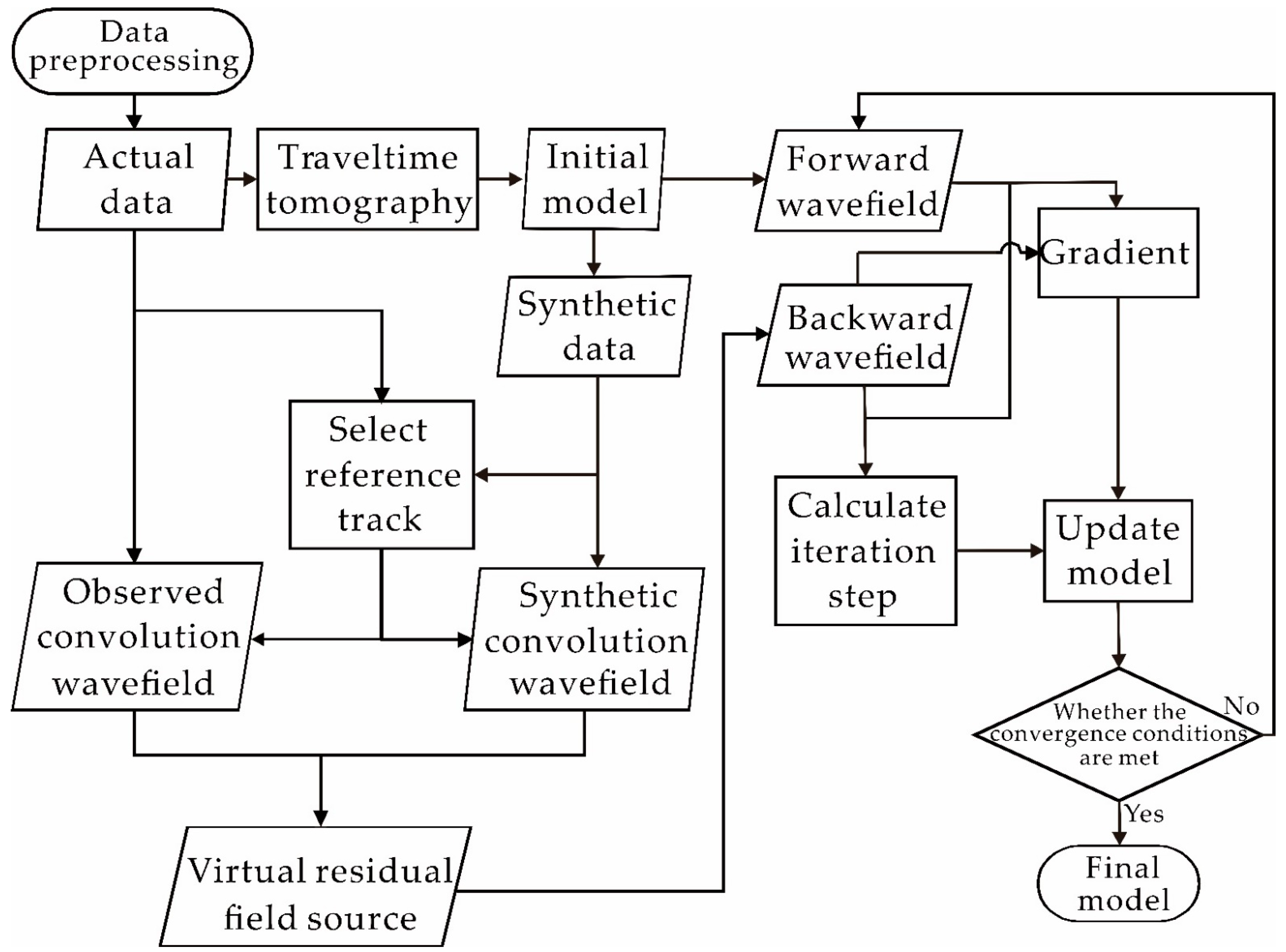
In this study, we use a source-independent waveform inversion method based on the envelope objective function (SIEWI) to invert cross-hole GPR data in the time domain. SIEWI has a successful application experience in the seismic field [
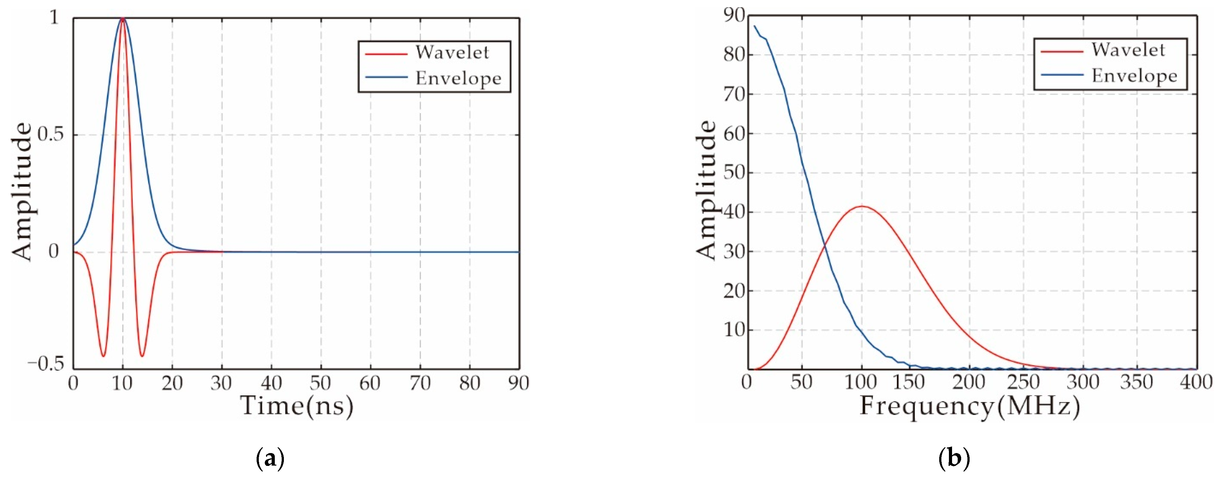
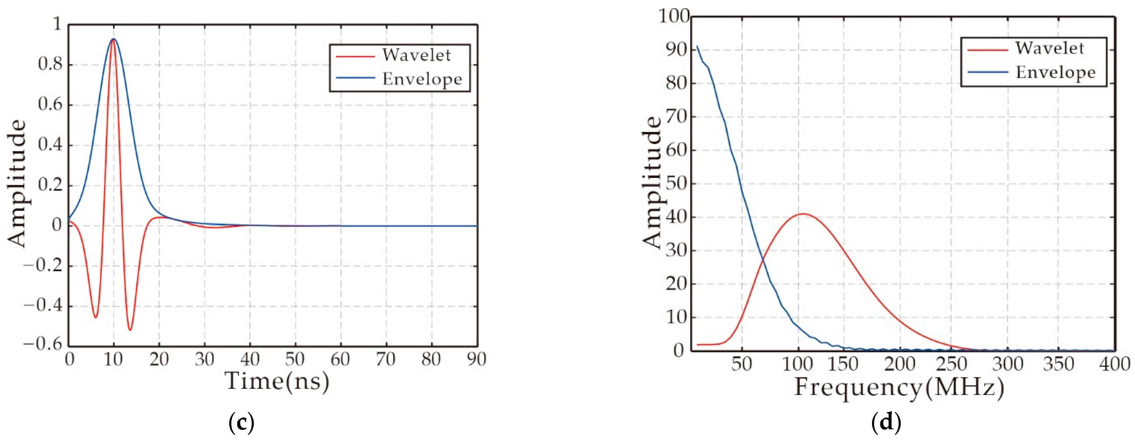
37]. In this paper, the gradient and step size equations of SIEWI are re-derived for GPR in the time domain, and the dual-parameter simultaneous inversion of permittivity and conductivity is achieved. First, we convolve the real data with a reference trace from the forward data. Similarly, we convolve the forward data and a reference trace from the real data, and simultaneously, take the envelope of the two sets of convolution results to establish a new objective function. In theory, the new convoluted wavefield shares the same source wavelet, regardless of the excitation pulse used in the forward process. Another important feature of the new objective function is that the source wavelet used in the forward wavefield plays a filtering role on the convolutional wavefield. The envelope transform can effectively restore the low-frequency information of the data and can suppress the local minimum, which further guarantees the effectiveness of the method. For the forward modeling in the inversion processing, we solve Maxwell’s equation for the transverse electric (TE) mode by using the 2D finite-difference time-domain method (FDTD) with the convolutional perfected marched layer (CPML) absorbing boundary condition [38]. This paper applies this method to synthetic data and real data to test its effectiveness.

2. Methods

2.1. Derivation of the Objective Function

The objective function for conventional time-domain full waveform inversion is the l2 norm between the real and forward data.
S = 1 2 i n s j n r | | E i , j ε , σ E i , j o b s | | 2 ,
In Equation (1), E(ε,σ) and Eobs are synthesized data and real data, respectively, and the value of the objective function is the sum of the residuals on all transmitters (indicated by i), receivers (indicated by j) and the observation time (indicated by τ). The electric field of the ground penetrating radar can be considered as the convolution of the source wavelet and Green’s function g, so the objective function can be rewritten as follows:
S = 1 2 i n s j n r | | g i , j f o r s f o r g i , j o b s s o b s | | 2 ,
where for corresponds to the synthesized data E(ε,σ); obs corresponds to the observed data Eobs; * is the convolution operator. Before inverting the real data, a very important step is to estimate the source wavelet sobs of the real data. Since there may be problems with real data quality, the source wavelets estimated from each signal are often inconsistent. There are unavoidable differences in amplitude and phase between each wavelet. For data with poor signal-to-noise ratio, this difference will be very large. This increases the difficulty of estimating the source wavelet, so the process of estimating the source wavelet often consumes a lot of time and has potential errors.
In order to avoid the above problems, this paper adopts a waveform inversion method that does not depend on the source wavelet. The objective function of this method is:
S = 1 2 i n s j n r | | E i , j ε , σ E i , k o b s E i , j o b s E i , k ε , σ | | 2 ,
where k is the reference trace selected according to the situation. Rewrite Equation (3) into a convolution form, such as Equation (2):
S = 1 2 i n s j n r | | g i , j f o r g i , k o b s s f o r s o b s g i , j o b s g i , k f o r s f o r s o b s | | 2 ,
Equation (4) is similar to Equation (2), and it can be seen that the two items in the objective function have the same source wavelet. Therefore, no matter what kind of source wavelets are provided for forwarding modeling in inversion, the purpose of waveform inversion can be achieved. The full waveform inversion based on the new objective function Equation (3) does not depend on the accurate source wavelet. For traditional FWI, the inaccurate source wavelet has a great influence on the inversion.
In this paper, the objective function of SIEWI is modified using the envelope algorithm to suppress local minima, further guaranteeing the effectiveness of the method. The objective function is given in Equation (5):
S = 1 2 i n s j n r | | E c E c o b s | | 2 ,
where Ec is the envelope of the simulated convolution wavefield, and E c o b s is the envelope of the observed convolution wavefield. Their corresponding expressions are:
E c = ( E i , j E i , k o b s ) 2 + H ( E i , j E i , k o b s ) 2 ,
E c o b s = ( E i , j o b s E i , k ) 2 + H ( E i , j o b s E i , k ) 2 ,
H denotes the Hilbert transform operator. Since the new objective function is composed of two envelopes in Equation (3), the waveform inversion method based on Equation (5) still uses the same source wavelet ( s f o r s o b s ).

2.2. Gradient

The gradient is obtained by deriving the objective function (5) with the model parameter p:
S p = i n s j n r E c p E c o b s p r i , j ,
where
r i , j = E c E c o b s ,
E c p = 1 E c E i , j E i , k o b s ( E i , j p E i , k o b s ) + H E i , j E i , k o b s ( h E i , j p E i , k o b s ) ,
E c o b s p = 1 E c o b s E i , j o b s E i , k ( E i , k p E i , j o b s ) + H E i , j o b s E i , k ( h E i , k p E i , j o b s ) ,
Putting Equations (9)–(11) into Equation (8) and sorting out:
S p = i n s j n r E c E c o b s E c E i , j E i , k o b s E i , j p E i , k o b s + H E i , j E i , k o b s h E i , j p E i , k o b s i n s j n r E c E c o b s E c o b s E i , j o b s E i , k E i , k p E i , j o b s + H E i , j o b s E i , k h E i , k p E i , j o b s ,
For the convenience of equation derivation, the above equation is divided into four parts and the equations are:
r 1 = i n s j n r E c E c o b s E c ( E i , j E i , k o b s ) ( E i , j p E i , k o b s ) ,
r 2 = i n s j n r E c E c o b s E c H E i , j E i , k o b s ( h E i , j p E i , k o b s ) ,
r 3 = i n s j n r E c E c o b s E c o b s E i , j o b s E i , k ( E i , k p E i , j o b s ) ,
r 4 = i n s j n r E c E c o b s E c o b s H E i , j o b s E i , k ( h E i , k p E i , j o b s ) ,
In the above Equation (13), the product of the first two items is represented by r 1
r 1 = E c E o b s E c E i , j E i , k o b s ,
After sorting, Equation (13) can be written in integral form:
E i , j p E i , k o b s r 1 = [ E i , j p t τ E i , k o b s τ r 1 t ] d τ d t ,
Let t τ = ξ ; then d τ = d ξ can be rewritten as:
E i , j p E i , k o b s r 1 = E i , j p ξ E i , k o b s t ξ r 1 t d t d ξ = E i , j p ξ r 1 ξ d ξ ,
r 1 ξ is the cross-correlation between the residual and the real data reference trace, which represents the backward residual field source of Equation (13):
r 1 = E i , k o b s ( E c E o b s E c E i , j E i , k o b s ) ,
Equation (19) is a simplified form of Equation (18). It can be seen that Equation (19) is the result of the dot multiplication between the first-order partial derivative ( E i , j p ) and the cross-correlation residual ( r 1 ) of the electric field to the model parameters, which is similar to the gradient equation for waveform inversion under the traditional objective function. In Equation (19), r is the backward residual field source derived in Equation (13). After rearranging, Equation (19) is rewritten as:
( E i , j p E i , k o b s ) r 1 = [ v i , x E ξ τ g x , j E τ d τ ] r 1 ξ d ξ ,
Since the transmitters represented by the virtual source vector v i , x are forward, and the receivers represented by Green’s function g x , j are reverse in time series, the subscripts of the two are not the same, and the order is opposite to correspond to the time series. Set ξ τ = t ; then d τ = d t . Equation (21) can be rewritten as:
E i , j p E i , k o b s r 1 = v i , x E t g x , j E ξ t d t r 1 ξ d ξ = v i , x E t [ g x , j E ξ t r 1 ξ d ξ ] d t ,
g ξ t r ξ d ξ represents the backward propagation field with the opposite time series, and Equation (22) is the zero-phase convolution of the virtual source and the backward propagation field. According to Equation (22), the gradient expressions of permittivity and conductivity are given in this paper:
S ε S σ = i n s τ n t ( t E s ) T G ^ T R s ( E s ) T G ^ T R s ,
in which G ^ T R s can be interpreted as a backward propagating vector field in the same medium, where:
R s = j = 1 n r r 1 ,
Then, Equations (14)–(16) are derived in the same way as formula (13). Then, we can obtain the remaining three components of the backward residual field source corresponding to Equation (12), which are:
r 2 = E i , k o b s H E c E o b s E c H ( E i , j E i , k o b s ) ,
r 3 = E i , j o b s ( E c E c o b s E c o b s E i , k E i , j o b s ) ,
r 4 = E i , j o b s H E c E c o b s E c o b s H ( E i , k E i , j o b s ) ,
where r and r 2 denote the adjoint sources at any detection point j; r 3 and r 4 denote the adjoint sources at the reference trace k. Subsequently, we merge r and r 2 to obtain the backward residual field source r 12 ; r 3 and r 4 merge to obtain the backward residual field source r 34 . The equations of r 12 and r 34 are:
r 12 = E i , k o b s E c E o b s E c E i , j E i , k o b s H E c E o b s E c [ H ( E i , j E i , k o b s ) ] ,
r 34 = E i , j o b s E c E c o b s E c o b s E i , k E i , j o b s H E c E c o b s E c o b s [ H ( E i , k E i , j o b s ) ] ,
In Equations (28) and (29), denotes the cross-correlation operator. What needs to be noticed is the changes in the subscripts of Equations (28) and (29). The reference trace in r 12 is selected from the observation data; the reference trace needs to be selected according to the actual situation before inversion. Usually, the reference trace is the one closer to the transmitter or replaced by averaging traces. The reference trace in r 34 is selected from synthetic data. During the inversion, synthetic data need to be superimposed; the final superimposed data are used as one trace to perform a cross-correlation operation with the actual data.
Finally, we give the gradient of permittivity and conductivity:
S ε x S σ x = s 0 T d t ( t E x , t d τ T s , d , τ x , t ) 0 T d t ( E x , t d τ T s , d , τ x , t ) ,
where
T s , d , τ x , t = G x , τ t , x j , 0 r 12 + r 34 ,
T is the backward propagation field, and it can be seen that r 12 and r 34 are jointly used as the residual field source.

2.3. Step Calculation

In the iteration, the conjugate gradient method is used to update the permittivity and conductivity at the same time [39]:
ε x k + 1 = ε x k ζ ε , k C ε x k ,
σ x k + 1 = σ x k ζ σ , k C σ x k ,
where C ε x k and C σ x k are the gradient directions of the permittivity and conductivity during the kth iteration, respectively. ξ ε , k and ξ σ , k are the iteration steps corresponding to gradients C ε x k and C σ x k , respectively. The calculation equation for conjugate gradient is:
ε x k + 1 = ε x k ζ ε , k C ε x k ,
σ x k + 1 = σ x k ζ σ , k C σ x k ,
When k = 1, the gradients of the two are C ε x 1 = S ε x 1 and C σ x 1 = S σ x 1 , respectively. Introducing the conjugate gradients C ε and C σ simultaneously updating the permittivity and conductivity of the model at the same time, we can give the error calculation method at the k + 1 iteration:
S p k + 1 = S p k + ζ k C p k = S ε k + ζ ε , k C ε k , σ k + ζ σ , k C σ k ,
This method finds the optimal step size ζ, that is, searches for the minimum value of the objective function along the gradient direction, where ε and σ denote permittivity and conductivity, respectively. C p n is the gradient of the k-th iteration. Since the above three are fixed, the minimum value can be reached by setting the first derivative to zero:
S ε k + ζ ε , k C ε k , σ k + ζ σ C σ k ζ k = 0 ,
According to the optimal step length equation of the conventional GPR full waveform inversion method [40], we give the best step length equation suitable for SIEWI to update the permittivity and conductivity at the same time:
ζ ε , k = κ ε s d τ γ ε r e n v s d τ γ ε γ ε ,
ζ σ , k = κ σ s d τ γ σ r e n v s d τ γ σ γ σ ,
with
r e n v = E i , j E i , k o b s e n v E i , j o b s E i , k e n v ,
γ ε = E i , j d i s ε E i , k o b s e n v E i , j E i , k o b s e n v E i , k d i s ε E i , j o b s e n v E i , k E i , j o b s e n v ,
γ σ = E i , j d i s σ E i , k o b s e n v E i , j E i , k o b s e n v E i , k d i s σ E i , j o b s e n v E i , k E i , j o b s e n v ,
In the equation, env denotes the envelope transformation of the convolution wavefield. κε and κσ are small stability factors specified according to the magnitude of the gradient extreme value during the step calculation. When the stability factor is within a reasonable order of magnitude, the iteration can guarantee stability, and it changes continuously as the iteration progresses.

3. Inversion Strategy

3.1. Convolution Wavefield Characteristics

As shown in Equation (3), the forward convolution wavefield of SIEWI is obtained by convolution between synthetic data and real data. If the frequency bands of the synthesized data and real data are inconsistent during convolution, the frequency band range of the wavefield after convolution will change. In order to illustrate this phenomenon, an example of synthetic data is used for analysis in this paper. The frequency band variation in the convolutional wavefield is simulated when source wavelets with different center spectra are used in the inversion process. Figure 1a is the original waveform of the simulated observation data in this article, with a center frequency of 100 MHz; Figure 1d is the frequency spectrum of the wavelet. The source wavelet used in the inversion process is shown in Figure 1b; the selected wavelet is the Ricker wavelet with a center frequency of 60 MHZ; Figure 1e is the corresponding frequency spectrum of the Ricker wavelet. Figure 1c is a waveform selected from the trace set of the residual field source obtained when the above source wavelet is used for inversion; Figure 1f is its frequency spectrum. It can be seen that the center frequency of the residual field source is between 60 MHz and 100 MHz, and the frequency band is close to the intersection of the two frequency bands in Figure 1d,e.
In order to verify the frequency characteristics of the wavelet after convolution, we conducted a second set of time–frequency analyses. As shown in Figure 2, the comparative analysis method is the same as Figure 1, except that the center frequency of the Ricker wavelet is 140 MHz. By observing the spectrum of the residual field source in Figure 2f, it is noticed that the spectrum of the residual field source is shifted again, the center frequency is between 100 MHz and 140 MHz and the frequency band is close to the intersection of the two frequency bands of Figure 2d,e.
According to this feature of the convolution operation, we can invert the frequency information of a specific range of the original data by changing the center frequency of the source wavelet used in the inversion. It should be noted that the convolution transformation of the wavelet may cause the loss of low-frequency information. As shown in Figure 1f and Figure 2f, the low-frequency region of the wavelet spectrum after convolution is significantly less than that of two wavelets. The lack of low-frequency information will not only adversely affect the restoration of the model’s long-wavelength information, but also cause the inversion to fall into a local extreme. Therefore, we use envelope transformation to optimize the objective function. The envelope can not only restore long-wavelength information, but also increase the robustness of the inversion. Figure 3 shows the spectrum change after envelope transformation of the Ricker wavelet after the low-frequency information is filtered by the high-pass filter. According to the principle of the multi-scale FWI strategy, the multi-scale strategy for SIEWI can be realized by selecting the center frequency of the source wavelet in the order from low to high during the inversion process.

3.2. Multi-Scale SIEWI Strategy

Developing a multi-scale inversion strategy is an effective way to reduce the dependence of waveform inversion on the initial model and the problem of nonlinearity in waveform inversion. In this paper, the idea of developing an inversion strategy for SIEWI is to separate the frequency components of the inversion information. Low-frequency components are preferentially inverted to restore long-wavelength components. Then, in the iteration, the target frequency components of the inversion information are gradually increased to obtain high-resolution SIEWI results. The specific implementation method is to select the source wavelet with a lower center frequency as the source wavelet required for forward modeling. It has been demonstrated that the frequency range of the residual field source can be controlled indirectly by changing the source wavelet frequency through spectral analysis of the convolutional wavefield. When the source wavelet with a lower center frequency is selected for inversion, the inversion is mainly for the low-frequency information in the actual data. As the iteration proceeds, the center frequency of the source wavelet required for forward modeling is gradually increased, thereby realizing a multi-scale inversion strategy from low frequency to high frequency. The source-independent wavelet waveform inversion method can effectively prevent the initial wavelet waveform mismatch caused by changing the wavelet frequency and ensure the effectiveness of the strategy.
The waveform inversion method has a high dependence on the initial model, and the real data inversion has problems such as relatively low data signal-to-noise ratio and strong nonlinearity. In order to obtain good inversion results, a relatively accurate initial model is usually provided for the inversion. In this paper, the results obtained by the ray-based method are used as the initial models to formulate a SIEWI strategy that does not require source wavelet estimation (as shown in Figure 4). In the SIEWI inversion, the Ricker wavelet with the center frequency from low to high is selected as the source wavelet for forward modeling. Since the source wavelet required for SIEWI forward modeling does not cause adverse effects on convergence, the source wavelet waveform and flexible center frequency of the wavelet can be selected arbitrarily.

4. Results

4.1. Synthetic Data Verification

In order to verify the inversion capability of SIEWI, we simulated a two-dimensional model when the cross-hole structure is a homogeneous medium and the anomalous body is two pipelines. As shown in Figure 5, the model has a dimension of 8 m in both the x and y directions. In the homogeneous medium, there are two pipeline abnormal bodies buried with a diameter of 0.5 m. The relative permittivity and conductivity of the two anomalies located at the positions of (2 m, 3 m) and (4 m, 3 m) are 7 and 0.008 S/m, respectively. The relative permittivity and conductivity of the top- and bottom-layer medium are both 5 and 0.001 S/m, respectively. The relative permittivity and conductivity of the mid-layer medium are 5.5 and 0.0028 S/m, respectively. In this example, a total of 13 transmitter positions (represented by circles) and 13 receiver positions (represented by crosses) are included, and both the transmitter interval and the receiver interval are 0.5 m. The center frequency of the source wavelet used in the synthesized data is 150 MHz, the waveform is the first-order integral form of the Ricker wavelet and the maximum amplitude is two.
According to SIEWI’s inversion strategy, we use the ray-based inversion result as the initial model of the inversion (Figure 6). In order to compare the difference between FWI and SIEWI inversion when the wavelet is wrong, we choose to use an inaccurate source wavelet for FWI and SIEWI during the inversion, respectively. The source wavelet is a Ricker wavelet with a center frequency of 100 MHz and a maximum amplitude of one, which differs from the exact source wavelet in both amplitude and frequency.
In order to prove that SIEWI can completely ignore the adverse effects of source wavelets in the inversion process, we construct a special case where source wavelets are very unfavorable for waveform inversion. The source wavelet used in the inversion is different from the original data source wavelet in waveform, frequency and maximum amplitude. When using inaccurate source wavelets, even if the initial model uses relatively accurate ray results as the initial model, traditional FWI still cannot obtain the desired results (Figure 7a,b). If a uniform initial model is used, the traditional full waveform inversion method will have higher nonlinearity and will be more likely to fall into a local minimum. Inaccurate source wavelets will have a greater impact on the inversion. In this paper, SIEWI is used to invert the cross-hole GPR data, and the waveform inversion is realized in the absence of prior information, including the source wavelet. Relevant synthetic data inversion experience can be applied to process actual data to realize a waveform inversion strategy that does not require clear source wavelet conditions and source wavelet estimation. Among them, the selection of reference traces and the establishment of multi-scale inversion strategies are the key issues of this method.
Theoretically, the choice of reference traces has little effect on the inversion results. However, in practical applications, we find that the use of different reference traces has different effects on the final inversion results, so we usually choose the average trace or the trace near the transmitter as the reference trace. In this paper, we chose to use the nearby channel as the reference channel. Furthermore, to construct a multi-scale inversion strategy, we exploit the properties of convolutional wavefields. In the inversion, the Ricker wavelet of the stepped center frequency is used as the source wavelet required by the forward part. For example, when the model in Figure 5 is used for verification, the source wavelet frequency corresponding to the synthesized data is 150 MHz. In the inversion, the source wavelet frequencies used are 60 MHz, 100 MHz, 140 MHz and 200 MHz. It is worth noting that our method does not rely on the exact source wavelet, but the source wavelet still needs to be provided for forward inversion during the inversion process. In principle, the source wavelet morphology has no effect on the inversion, which is also confirmed in practical applications. By selecting source wavelets in different frequency ranges, a set of frequency inversion strategies from low frequency to high frequency are formed.
Figure 7c,d are the relative permittivity and conductivity results obtained using SIEWI, respectively. It can be seen that, whether it is the interface of the three layers or the two anomalies in the middle, the position information and physical parameters correspond well to the original model, especially being that the conductivity is basically consistent with the original model. The near-source anomalies in traditional FWI (Figure 7a,b) disappear completely, and it can be considered that the new method eliminates the adverse effects of inaccurate source wavelets. At the same time, the synthetic verification adopts the envelope objective function, which has a good suppression effect on the local minimum. It can be seen from the inversion results that the false anomalies are basically eliminated in the inversion results.

4.2. Observation Data Inversion

Xiuyan jade, produced in Xiuyan County, Liaoning Province, China, is one of the four famous jades in China. King Jade, the largest jade body in the world, is a broken jade body located on a mountain (see Figure 8). The local government plans to build a tourist attraction based on jade culture there. The investigation site was located at the foot of King Jade. The purpose of the investigation is to evaluate the stability of the underground foundation, find out the possible location of the mined-out area, find out the filling conditions of the underground pore space and prevent further collapse and rolling of the jade body.
In the fieldwork, the acquisition system selects an antenna with a center frequency of about 100 MHz. The horizontal distance between the boreholes is 16 m. Originally, the length of each borehole was more than 100 m, but it became shallower due to bottom material filling. Metal casings are used in the upper part of both boreholes. Therefore, the detectable range of the radar is shortened. From a depth of 36.5 m to 67.5 m, there are a total of 32 source locations, separated by 1 m. Each source location corresponds to a total of 28 receiving locations, separated by 1 m. For the first source at 36.5 m, the receiver starts at 23.5 m and moves down to 50.5 m. For the next source position, the receiver scan range is moved down 1 m. Figure 9 shows the raw data measured on-site.
When inverting real data, traditional FWI needs to estimate the source wavelet before the inversion starts and then use the estimated source wavelet to synthesize the data when forwarding the initial model. In order to ensure the accuracy of the source wavelet, it is usually necessary to estimate the source wavelet for each source at the launch position. Here, we use the collected data to estimate the source wavelet according to the deconvolution technique [14]. This set of data corresponds to 32 source positions, so after the source wavelet estimation, 32 source wavelet waveforms will be obtained. Although the locations of the transmitter are different, since the source wavelet is transmitted in the boreholes by the same radar system, the source wavelet waveform should theoretically be the same. In fact, the estimated source wavelet waveforms are not consistent. When we use the deconvolution technique to estimate the source wavelet, due to the different distances between the source wavelet and the receiver, the source wavelet amplitude estimated from different channel data has a huge difference. When the distance between the transmitting source and the receiving antenna is relatively smaller, the estimated source wavelet amplitude is larger. Taking the Xiuyan data as an example, for the 32 source wavelets estimated from the first source position, the maximum amplitude value is about 200 times the minimum amplitude value, and the true amplitude value cannot be accurately obtained. Since there is only one source wavelet required in the inversion process, only the maximum amplitude value can be used as the source wavelet amplitude in real operation, and this amplitude cannot be consistent with the real source wavelet amplitude. Due to the large difference in waveform amplitudes, it is inconvenient to display them in one graph. Here is a comparison chart of 32 estimated source wavelets after the source wavelet amplitude is normalized. As shown in Figure 10, it can be seen that even if the difference in amplitude is eliminated, there are still obvious differences in the waveform of different source wavelets. Only one fixed source wavelet can be used in the forward part of the inversion process. The selection of this source wavelet is extremely difficult. In order to invert real data, we can only select source wavelets with similar waveforms and normalize them to take averaging channel as the source wavelet for inversion, but this method cannot guarantee the accuracy of the estimated source wavelet. The amount of actual ground penetrating radar data is large, and the source wavelet estimation process will reduce the inversion efficiency. Moreover, with the increase in iterations, the source wavelet needs to be re-estimated and repeatedly verified because the source wavelet estimation needs to forward the initial model. Therefore, as the initial model is updated, the result of the source wavelet estimation will also change. This process needs to be performed manually, which is time-consuming and requires a professional operation.
In the entire inversion process, we only provide the Ricker wavelet as the source wavelet required for the forward part, and continuously increase the center frequency of the Ricker wavelet in the iteration to realize the multi-scale inversion strategy designed in this article for inversion.
Figure 11 shows the ray-based inversion results of the “Jade Emperor” foundation data. Among them, the ray-based dielectric permittivity inversion results can better restore the formation information, which is because the theory of traveltime tomography is relatively complete, but the resolution of the ray theoretical inversion results is lower than that of the waveform inversion results. In addition, attenuation tomography based on maximum amplitude can only restore the conductivity distribution to some extent, which is also the current status of tomography, and cannot give reliable conductivity inversion results. This paper uses the inversion results of permittivity and conductivity based on ray theory as the initial model for waveform inversion and proves that SIEWI can achieve effective inversion of real data.
In addition to resolution, the main advantage of the waveform inversion method over the ray-based inversion method is that it can simultaneously provide high-quality relative permittivity and conductivity inversion results. Due to the problems of multiple solutions and non-uniqueness in geophysical inversion, the inversion results usually require a combination of multiple methods to determine the real situation of the subsurface. Figure 12 shows the inversion results of the real Xiuyan data using the traditional full waveform inversion method and the SIEWI method. Both methods can reflect the distribution of the relative permittivity and conductivity of the foundation. From the inversion result in Figure 11, it can be seen that the inversion result of conductivity can match the result of permittivity in geological structures, which provides strong evidence for us to judge the underground situation. In addition, in the process of analyzing the permittivity results, there are some details that cannot be accurately determined, and the conductivity results provide a basis for judgment. For example, at a depth of 42 m, there is an unclear layer in the permittivity results, but in the conductivity results, the layer information of this position is obvious. The inversion results of FWI and SIEWI have high consistency, but there are still some differences. In terms of permittivity, the inversion results of FWI are similar to the inversion results of traveltime tomography, and the output results have little change compared with the initial model. However, there are some changes in the results output by SIEWI compared to the initial model. For example, for a layer with a depth of 48 m in the initial model, the relative permittivity increases significantly numerically after inversion by the SIEWI method. At the depth of 42 m, it is difficult to judge whether there is a layer only from the FWI results, but the SIEWI results can clearly see the existence of the layer. This conclusion can be verified by the conductivity results. In terms of conductivity, at a depth of 61.5 m, there is a suspected layer in the conductivity results of FWI, but no obvious layer is seen in the relative permittivity inversion results. The inversion results of SIEWI verify this hypothesis, and there is obviously a layer at 61.5 m in the conductivity results output by SIEWI.
The inversion results can fully demonstrate that SIEWI can effectively invert the real data. In real data inversion, the complex and unreliable process of source wavelet estimation can be completely ignored, which greatly improves the inversion efficiency and reduces the possibility of errors. The inversion results obtained by SIEWI can accurately describe the underground space structure and restore the horizon information that cannot be accurately inverted by ray theory and FWI.

5. Discussion

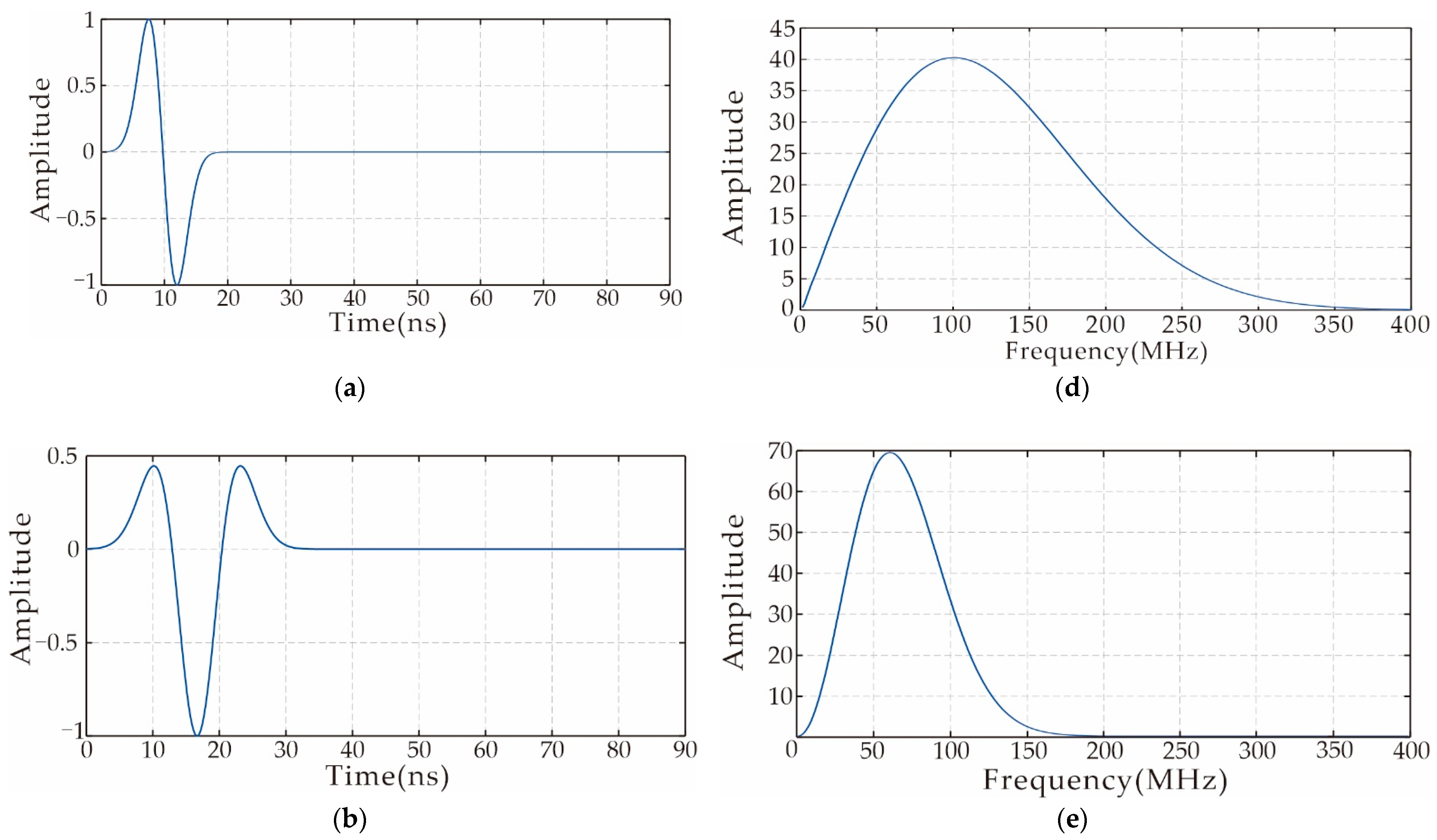
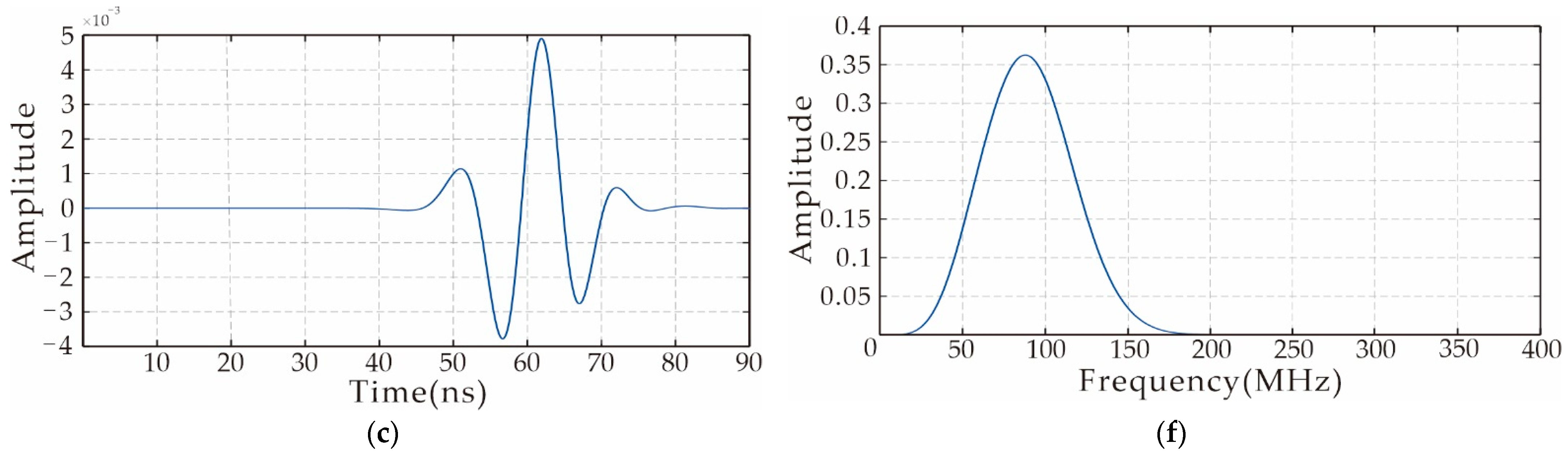
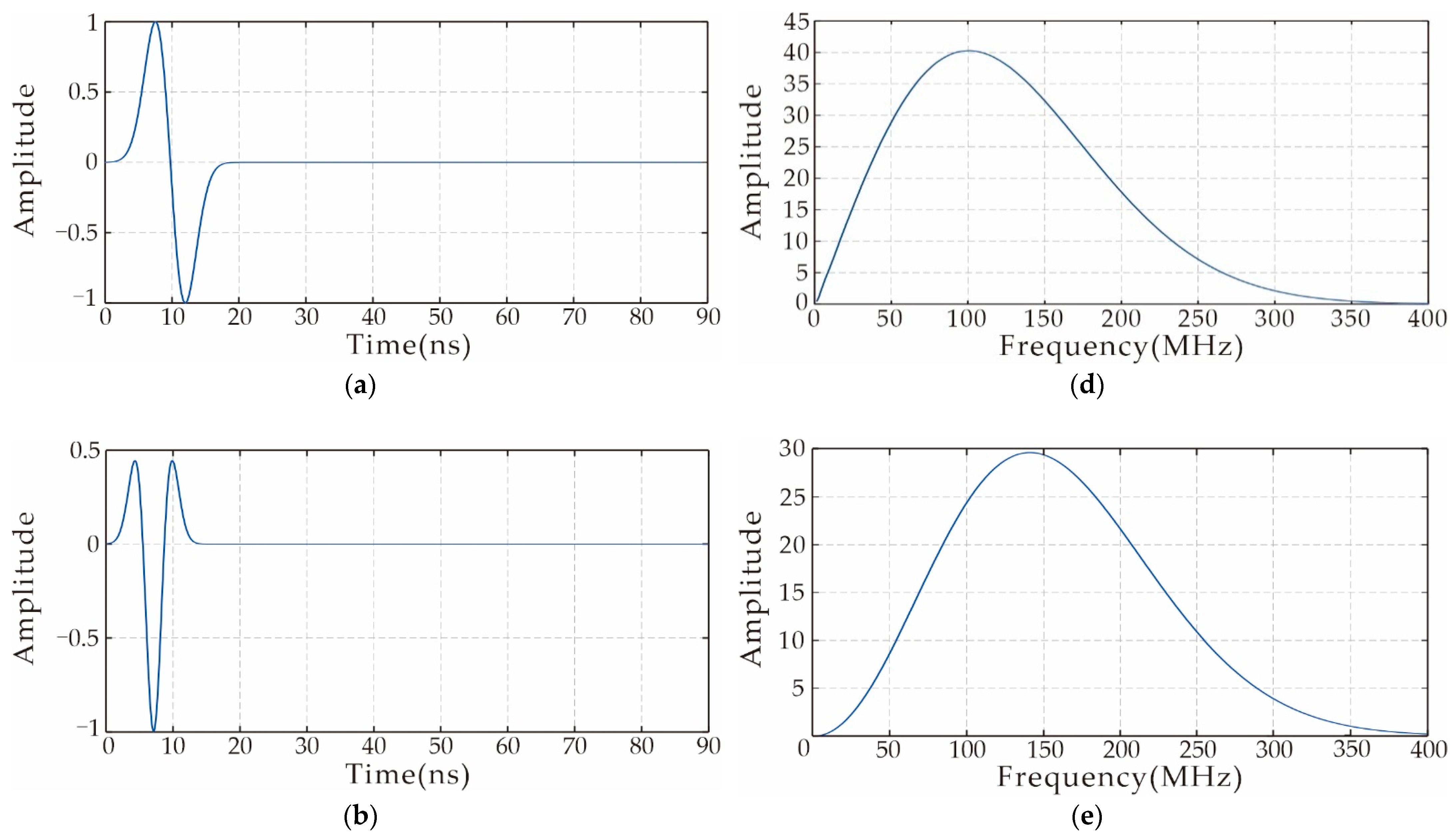
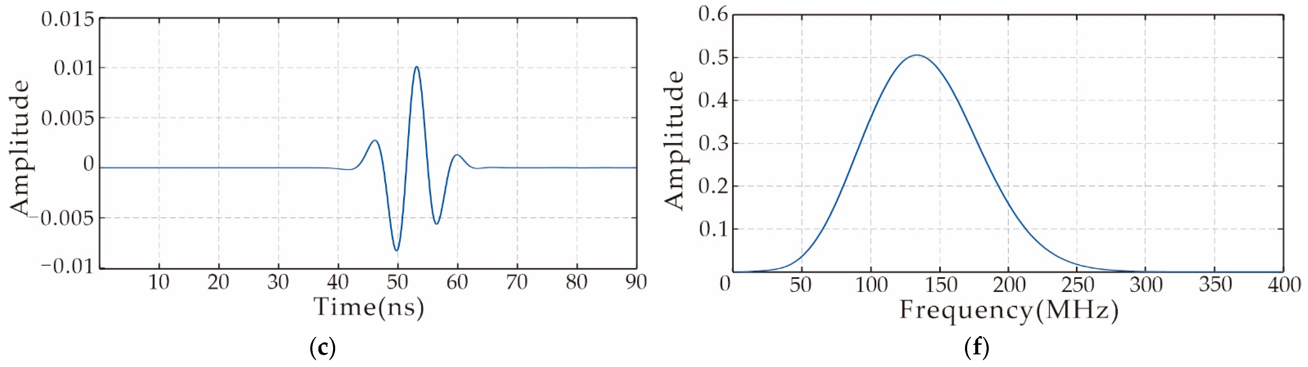
SIEWI is a waveform inversion method that does not rely on source wavelet in the inversion process. Because of this feature, it can ignore the important step of source wavelet estimation in the actual data inversion. In this paper, the SIEWI method is used to realize the inversion of synthetic data and actual data of cross-hole GPR. Compared with other waveform inversion methods, the biggest difference in SIEWI is that it does not need to estimate source wavelet at all. In actual data processing, source wavelet estimation is time-consuming and inaccurate. SIEWI avoids these problems. In order to make this method more suitable for inversion of cross-hole GPR in the time domain, we designed a multi-scale inversion strategy based on convolution. The envelope objective function is established by transforming the convolution wavefield, which can effectively solve the lack of low-frequency information caused by data acquisition and convolution operations. At the same time, the convolution and cross-correlation operations are nonlinear mathematical operations, which will increase the nonlinearity of the inversion. The envelope objective function can effectively suppress the nonlinear problem, avoid falling into a local minimum and make the inversion more stable. The convolution spectrum analysis proves that the frequency range of the residual field source can be controlled indirectly by changing the source wavelet frequency, and then a multi-scale inversion strategy suitable for SIEWI is established.
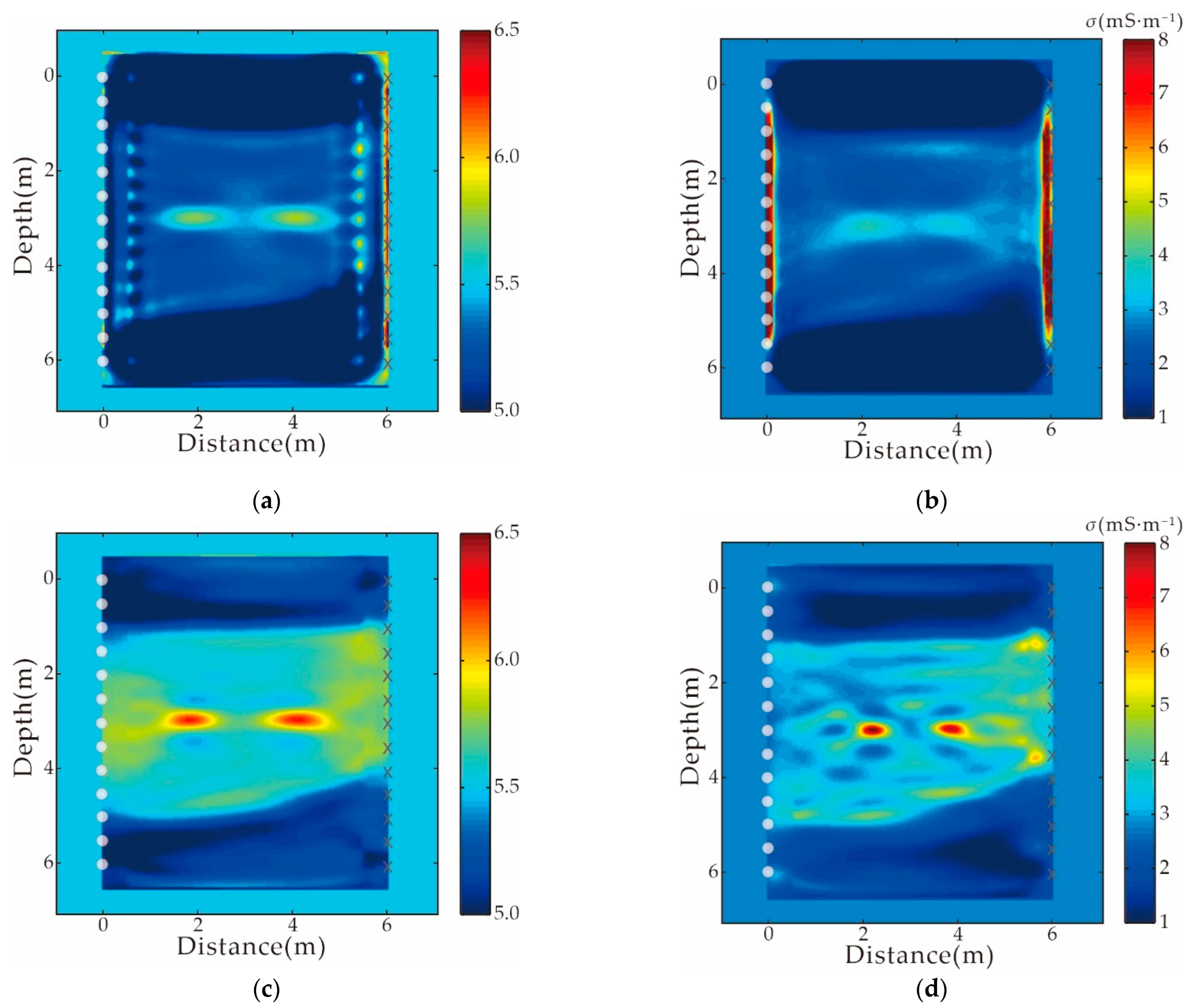
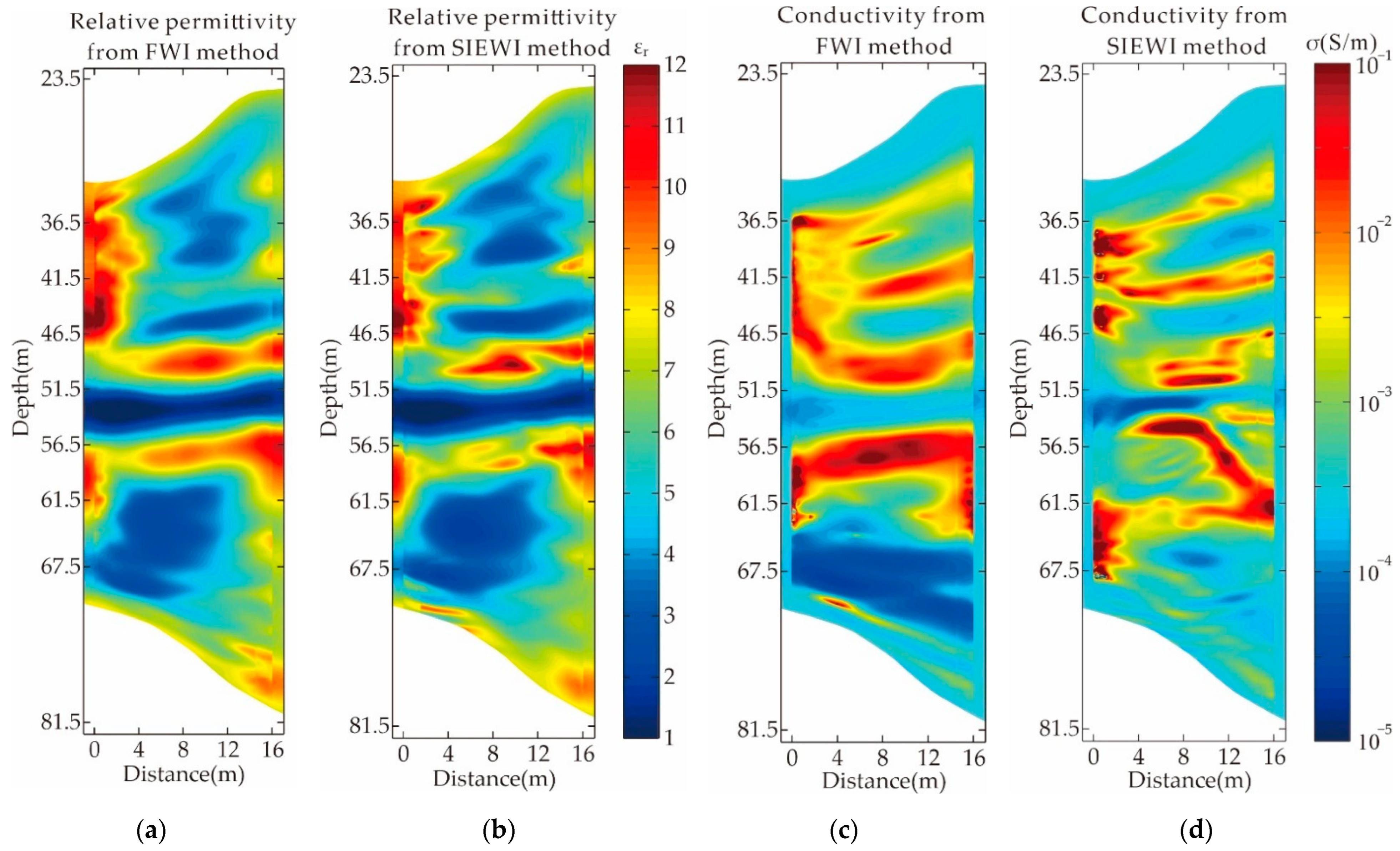
In this paper, SIEWI is used for the inversion of cross-hole ground penetrating radar data. The inversion capability of this method is verified by synthetic data, and it is proved that the accurate restoration of the cross-hole model can still be achieved when the source wavelet is wrong and the traditional FWI inversion cannot work. Compared with traditional FWI, SIEWI eliminates the complicated step of wavelet estimation which requires multiple manual interventions during the real data inversion. The efficiency of inversion is greatly improved. At the same time, it also avoids the serious impact on the inversion results if the source wavelet estimation is wrong. Comparing the inversion results of FWI and SIEWI, it shows that SIEWI has the ability to restore more stratigraphic information, especially to further verify the strata with doubts in the FWI results. The information is valuable for the prediction of unknown underground geological structures.
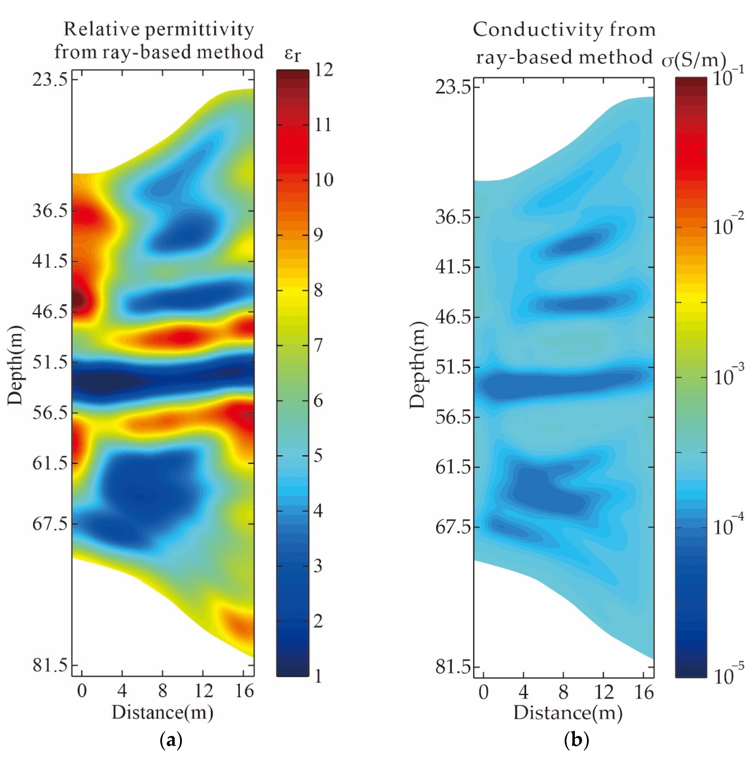
6. Conclusions

We successfully implemented a waveform inversion method that does not require source wavelets and applied it to cross-hole GPR data. For SIEWI, we derive in detail the gradient and step size required for the inversion. In the inversion, the characteristics of the convolution transform are fully utilized, and the multi-scale SIEWI strategy is established. In this paper, the tomographic inversion results are used as the initial model, and synthetic data and real data are inverted using SIEWI and FWI. Through synthetic data verification, SIEWI can realize the inversion of GPR cross-hole data, and it is proved that when the source wavelet is wrong and FWI cannot work, SIEWI can still work normally. In terms of actual data, the inversion results of SIEWI and FWI are relatively close on the whole, but there are some differences, which are mainly reflected in the conductivity results. There is horizon information in the SIEWI conductivity inversion results that was not obvious in the FWI results, and this horizon information has a certain reference value. In addition, the FWI inversion result is the best result obtained after multiple debugging, and in the entire iterative process, the source wavelet re-estimation is performed every ten iterations, requiring multiple manual interventions. However, SIEWI does not require manual intervention at all, and the inversion efficiency is greatly improved.

Author Contributions

Conceptualization, X.L. and S.L.; methodology, X.L. and S.L.; software, X.L. and X.M.; formal analysis, H.J., C.L. and H.L.; validation, H.J. and Z.F.; writing, X.L. and S.L.; funding acquisition, X.M., S.L. and C.L. All authors have read and agreed to the published version of the manuscript.

Funding

This research was funded by Science and Technology on Near-Surface Detection Laboratory under Grant 6142414200606 and the National Natural Science Foundation of China (Grant no. 42074146, 42001346).

Conflicts of Interest

The authors declare no conflict of interest.

References

  1. Daniels, D.J. Ground Penetrating Radar, 2nd ed.; The Institution of Engineering and Technology: London, UK, 2004. [Google Scholar]
  2. Liu, H.; Zhong, J.; Ding, F.; Meng, X.; Liu, C.; Cui, J. Detection of Early-stage Rebar Corrosion Using a Polarimetric Ground Penetrating Radar System. Constr. Build. Mater. 2022, 317, 125768. [Google Scholar] [CrossRef]
  3. Liu, H.; Shi, Z.; Li, J.; Liu, C.; Meng, X.; Du, Y.; Chen, J. Detection of road cavities in urban cities by 3D ground-penetrating radar. Geophysics 2021, 86, WA25–WA33. [Google Scholar] [CrossRef]
  4. Wang, F.; Liu, S.X.; Qu, X.X. Crosshole radar traveltime tomographic inversion using the fast marching method and the iteratively linearized scheme. J. Environ. Eng. Geophys. 2014, 19, 229–237. [Google Scholar] [CrossRef]
  5. Zhang, J.; Toksoz, M.N. Nonlinear refraction traveltime tomography. Geophysics 1998, 63, 1496–1823. [Google Scholar] [CrossRef]
  6. Olsson, O.; Falk, L.; Forslund, O.; Lundmark, L. Borehole radar applied to the characterization of hydraulically conductivity fracture-zones in crystalline rock. Geophys. Prospect. 1992, 40, 109–142. [Google Scholar] [CrossRef]
  7. Irving, J.D.; Knight, R.J. Effect of antennas on velocity estimates obtained from crosshole GPR data. Geophysics 2005, 70, K39–K42. [Google Scholar] [CrossRef]
  8. Zhou, H.; Sato, M. Subsurface cavity imaging by crosshole borehole radar measurements. IEEE Trans. Geosci.Remote Sens. 2004, 42, 335–341. [Google Scholar] [CrossRef]
  9. Liu, L.; Lane, J.W.; Quan, Y. Radar attenuation tomography using the centroid frequency downshift method. J. Appl. Geophys. 1998, 40, 105–116. [Google Scholar] [CrossRef]
  10. Williamson, P.R. A guide to the limits of resolution imposed by scattering in ray tomography. Geophysics 1991, 56, 202–207. [Google Scholar] [CrossRef]
  11. Williamson, P.R.; Worthington, M.H. Resolution limits in ray tomography due to wave behavior—Numerical experiments. Geophysics 1993, 58, 727–735. [Google Scholar] [CrossRef]
  12. Wu, R.S.; Toksoz, M.N. Diffraction tomography and multisource holography applied to seismic imaging. Geophysics 1987, 52, 11–25. [Google Scholar] [CrossRef]
  13. Virieux, J.; Operto, S. An overview of full-waveform inversion in exploration geophysics. Geophysics 2009, 74, WCC127–WCC152. [Google Scholar] [CrossRef]
  14. Tarantola, A. Inversion of seismic reflection data in the acoustic approximation. Geophysics 1984, 49, 1259–1266. [Google Scholar] [CrossRef]
  15. Tarantola, A. Linearized inversion of seismic reflection data. Geophys. Prospect. 1984, 32, 998–1015. [Google Scholar] [CrossRef]
  16. Tarantola, A. A strategy for nonlinear elastic inversion of seismic reflection data. Geophysics 1986, 51, 1893–1903. [Google Scholar] [CrossRef]
  17. Pratt, R.G. Seismic waveform inversion in the frequency domain. Part I: Theory and verification in a physical scale model. Geophysics 1999, 64, 888–901. [Google Scholar] [CrossRef]
  18. Pratt, R.G.; Shipp, R.M. Seismic waveform inversion in the frequency domain. Part 2: Fault delineation in sediments using crosshole data. Geophysics 1999, 64, 902–914. [Google Scholar] [CrossRef]
  19. Kuroda, S.; Takeuchi, M.; Kim, H.J. Full waveform inversion algorithm for interpreting cross-borehole GPR data. In Proceedings of the 2005 SEG Annual Meeting, Houston, TX, USA, 6–11 November 2005; pp. 1176–1179. [Google Scholar]
  20. Meles, G.A.; Van der Kruk, J.; Greenhalgh, S.A.; Ernst, J.R.; Maurer, H.; Green, A.G. A new vector waveform inversion algorithm for simultaneous updating of conductivity and permittivity parameters from combination crosshole/borehole-to-surface GPR data. IEEE Trans. Geosci. Remote Sens. 2010, 48, 3391–3407. [Google Scholar] [CrossRef]
  21. Ernst, J.R.; Maurer, H.; Green, A.G.; Holliger, K. Full-waveform inversion of crosshole radar data based on 2-D finite-difference time-domain solutions of maxwell’s equations. IEEE Trans. Geosci. Remote Sens. 2007, 45, 2807–2828. [Google Scholar] [CrossRef]
  22. Ernst, J.R.; Green, A.G.; Maurer, H.; Holliger, K. Application of a new 2D time-domain full-waveform inversion scheme to crosshole radar data. Geophysics 2007, 72, J53–J64. [Google Scholar] [CrossRef]
  23. Bunks, C.; Saleck, F.M.; Zaleski, S.; Chavent, G. Multiscale seismic waveform inversion. Geophysics 1995, 60, 1457–1473. [Google Scholar] [CrossRef]
  24. Meles, G.; Greenhalgh, S.; Van der Kruk, J.; Green, A.; Maurer, H. Taming the non-linearity problem in GPR full-waveform inversion for high contrast media. J. Appl. Geophys. 2012, 78, 31–43. [Google Scholar] [CrossRef]
  25. Fu, L.; Feng, Z.; Schuster, G.T. Multiscale phase inversion for 3D ocean-bottom cable data. Geophys. Prospect. 2020, 68, 786–801. [Google Scholar] [CrossRef]
  26. Fu, L.; Guo, B.; Sun, Y.; Schuster, G.T. Multiscale phase inversion of seismic data. Geophysics 2018, 83, R159–R171. [Google Scholar] [CrossRef]
  27. Choi, Y.; Alkhalifah, T. Source-independent time-domain waveform inversion using convolved wavefields: Application to the encoded multisource waveform inversion. Geophysics 2011, 76, R125–R134. [Google Scholar] [CrossRef]
  28. Lee, K.H.; Kim, H.J. Source-independent full-waveform inversion of seismic data. Geophysics 2003, 68, 2010–2015. [Google Scholar] [CrossRef]
  29. Bozdağ, E.; Trampert, J.; Tromp, J. Misfit functions for full waveform inversion based on instantaneous phase and envelope measurements. Geophys. J. Int. 2011, 185, 845–870. [Google Scholar] [CrossRef]
  30. Chi, B.; Dong, L.; Liu, Y. Full waveform inversion method using envelope objective function without low frequency data. J. Appl. Geophys. 2014, 109, 36–46. [Google Scholar] [CrossRef]
  31. Wu, R.S.; Luo, J.; Wu, B. Seismic envelope inversion and modulation signal model. Geophysics 2014, 79, WA13–WA24. [Google Scholar] [CrossRef]
  32. Fu, L.; Liu, L. Imaging the internal structure of trunks via multiscale phase inversion of ground-penetrating radar data. Interpretation 2021, 9, T869–T880. [Google Scholar] [CrossRef]
  33. Liu, X.; Liu, S.; Fu, L. Full Waveform Inversion of Cross-hole Radar Data Using Envelope Objective Function. In Proceedings of the 2018 17th International Conference on Ground Penetrating Radar, Rapperswil, Switzerland, 18–21 June 2018. [Google Scholar]
  34. Meng, X.; Liu, S.; Xu, Y.; Fu, L. Application of Laplace Domain Waveform Inversion to Cross-Hole Radar Data. Remote Sens. 2019, 11, 1839. [Google Scholar] [CrossRef]
  35. Edemsky, F.; Popov, A.; Zapunidi, S. A time domain model of GPR antenna radiation pattern. Int. J. Electr. Telecom. 2011, 57, 407–411. [Google Scholar] [CrossRef]
  36. Belina, F.A.; Irving, J.; Ernst, J.R.; Holliger, K. Waveform inversion of crosshole georadar data: Influence of source wavelet variability and the suitability of a single wavelet assumption. IEEE Trans. Geosci. Remote Sens. 2012, 50, 4610–4625. [Google Scholar] [CrossRef]
  37. Ao, R.D.; Dong, L.G.; Chi, B.X. Source-independent envelope-based FWI to build an initial model. Chin. J. Geophys. 2015, 58, 1998–2010. (In Chinese) [Google Scholar]
  38. Roden, J.A.; Gedney, S.D. Convolution PML (CPML): An efficient FDTD implementation of the CFS-PML for arbitrary media. Microw. Opt. Technol. Lett. 2000, 27, 334–339. [Google Scholar] [CrossRef]
  39. Liu, S.; Liu, X.; Meng, X.; Fu, L.; Lu, Q.; Deng, L. Application of Time-Domain Full Waveform Inversion to Cross-Hole Radar Data Measured at Xiuyan Jade Mine, China. Sensors 2018, 18, 3114. [Google Scholar] [CrossRef] [Green Version]
  40. Wu, J.; Liu, S.; Li, Y. Study of cross-hole radar tomography using full-waveform inversion. Chin. J. Geophys. 2014, 57, 1623–1635. [Google Scholar]
Figure 1. Convolutional spectrum analysis. (a) Source wavelet of real data: center frequency 100 MH and corresponding (d) spectrum; (b) source wavelet used in the forward modeling: center frequency 60 MHz and corresponding (e) spectrum; (c) a residual field source and the corresponding (f) spectrum.
Remotesensing 14 04878 g001aRemotesensing 14 04878 g001b
Figure 2. Convolutional spectrum analysis. (a) Source wavelet of real data: center frequency 100 MH and corresponding (d) spectrum; (b) source wavelet used in the forward modeling: center frequency 140 MHz and corresponding (e) spectrum; (c) a certain residual field source and the corresponding (f) spectrum.
Remotesensing 14 04878 g002aRemotesensing 14 04878 g002b
Figure 3. Spectrum analysis diagram before and after envelope transformation: (a) Ricker wavelet and its envelope; (b) spectra of Ricker wavelet and its envelope. (c) Ricker wavelet without low-frequency data and its envelope; (d) spectra of Ricker wavelet without low-frequency data and its envelope.
Remotesensing 14 04878 g003aRemotesensing 14 04878 g003b
Figure 4. Source-independent wavelet waveform inversion strategy for real data.
Remotesensing 14 04878 g004
Figure 5. The original model of synthetic data, the white circle represents the transmitter and the cross represents the receiver: (a) relative permittivity; (b) conductivity.
Remotesensing 14 04878 g005
Figure 6. The initial model based on ray theory: (a) relative permittivity; (b) conductivity.
Remotesensing 14 04878 g006
Figure 7. Inversion results using the wrong source wavelet. The traditional FWI obtains the (a) relative permittivity and (b) conductivity; SIEWI obtains the (c) relative permittivity and (d) conductivity.
Remotesensing 14 04878 g007
Figure 8. Field survey site and location map. The huge King Jade is located in the center of the photograph.
Remotesensing 14 04878 g008
Figure 9. Measured original data of Xiuyan foundation.
Remotesensing 14 04878 g009
Figure 10. Waveform comparison chart of 32 source wavelets after amplitude normalization.
Remotesensing 14 04878 g010
Figure 11. Inversion results of Xiuyan GPR data based on ray theory: (a) relative permittivity; (b) conductivity.
Remotesensing 14 04878 g011
Figure 12. Inversion results of real data from Xiuyan. Inversion results based on FWI: (a) relative permittivity and (c) conductivity; inversion results based on SIEWI: (b) relative permittivity; (d) conductivity.
Remotesensing 14 04878 g012
Publisher’s Note: MDPI stays neutral with regard to jurisdictional claims in published maps and institutional affiliations.

