
Mosaicking Weather Radar Retrievals from an Operational Heterogeneous Network at C and X Band for Precipitation Monitoring in Italian Central Apennines

 and
and
Abstract
:1. Introduction
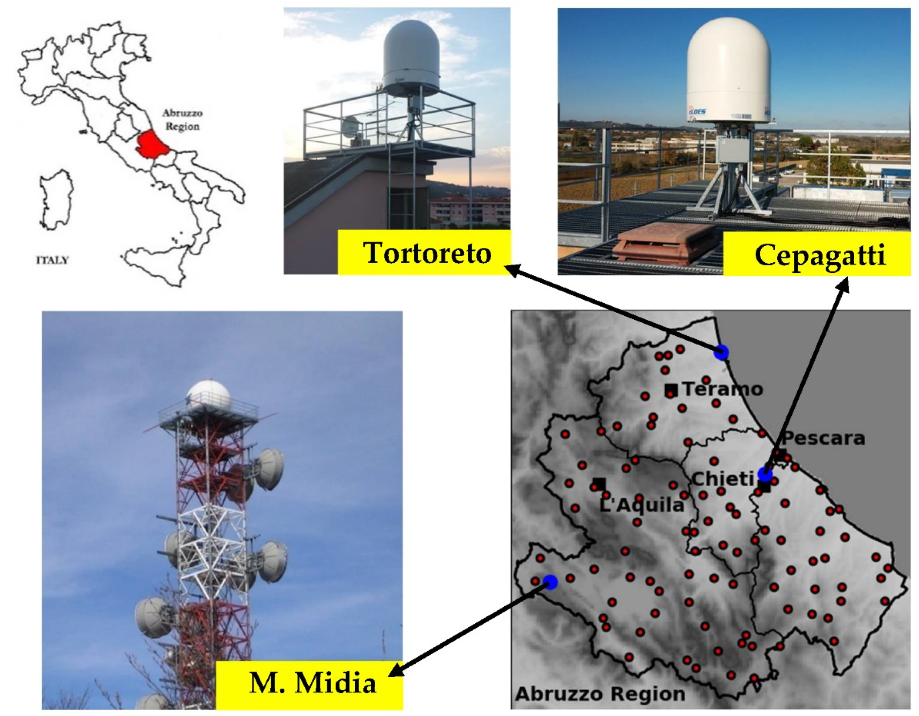
2. Abruzzo Region Weather Radar and Rain Gauge Network
2.1. C-band and X-band Weather Radars in Abruzzo
2.2. Rain Gauge Network in Abruzzo
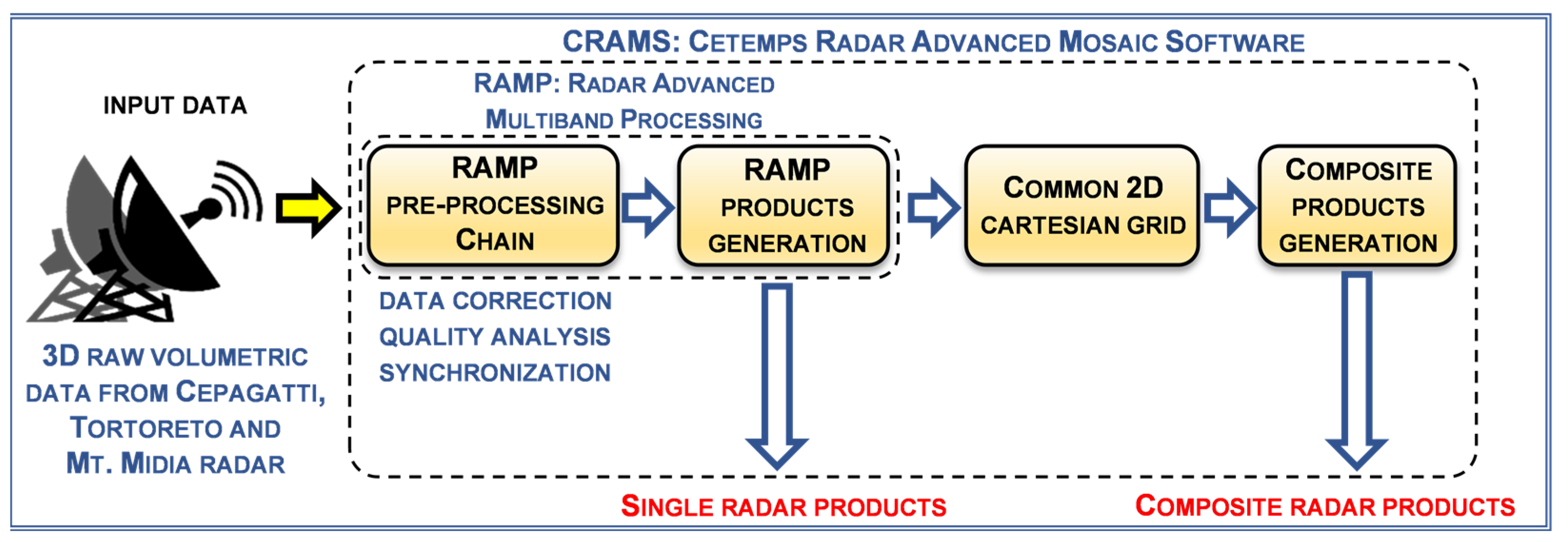
3. Single Radar and Mosaicking Methodology
- Coverage of a wider area of the monitored territory
- -
- overcoming the limited coverage of individual radars;
- -
- more accurate measurements at greater distances;
- Spatial redundancy of weather radar observations
- -
- inter-calibrating the hybrid network radars;
- -
- reducing ground clutter effects and beam blocking;
- -
- guaranteeing measurements even in the case of the failure of one radar;
- Mitigation of path attenuation effects and improved retrievals
- -
- reducing two-way path attenuation effects in complex orography;
- -
- extracting radar data in total signal extinction area;
- -
- improving the rainfall estimate thanks to simultaneous observations;
3.1. Single-Radar Algorithms
3.2. Radar-Gauge Spatial-Adjustment Methods
3.3. Radar Mosaicking Techniques
- Max, wherein a multi-radar maximum criterion is used;
- Avg, wherein a multi-radar average criterion is used;
- Lin, wherein a multi-radar linear distance-weighted criterion is used;
- Exp, wherein a multi-radar exponential distance-weighted criterion is used.
4. Mosaicking Validation Using Rain Gauge Data
| Mean error or error bias (optimum value = 0) | BiasR> = <(RWRNet−RRG)> |
| Error standard deviation STD (optimum value = 0) | |
| Absolute mean error (MAE) (optimum value = 0) | MAER|> |
| Root mean square error (RMSE) (optimum value = 0): | |
| Normalized RMSE (optimum value = 0): | |
| Fractional standard error (FSE) (optimum value = 0): | FSE = RMSE/<RRG> |
| Coefficient of correlation (Corr) (optimum value = 1): | Corr) |
| Mean–field ratio bias (MRB) (optimum value = 1): | MRB = <RWRNet>/<RRG> |
4.1. Overview of Selected Case Studies
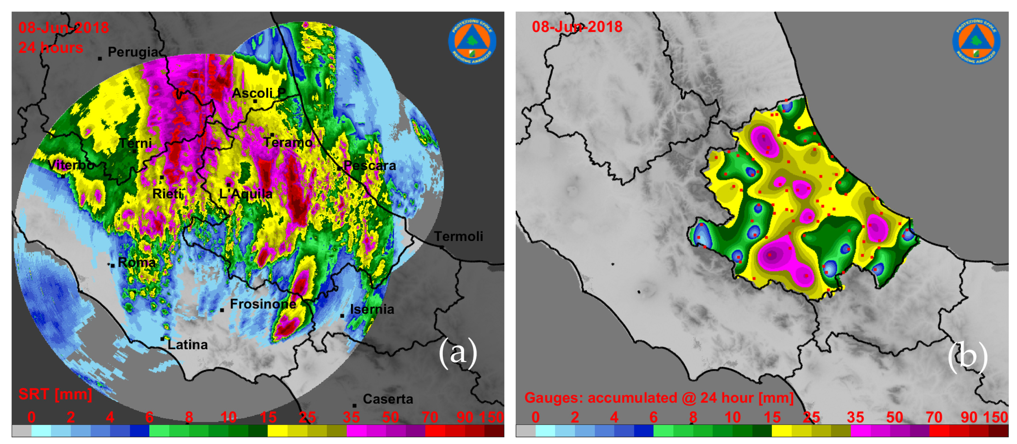
- Event on 8 June 2018. The first case corresponds to a strong inland atmospheric instability that developed into several convective precipitation phenomena. A minimum depression, located on the western Mediterranean, favored the transport of unstable currents over central and northern Italy, resulting in a phase of bad weather, rapidly evolving. It was characterized by precipitation with a predominantly rain shower or thunderstorm character, of strong intensity, with frequent electrical activity, local hail storms, and strong wind gusts.
- Event on 4 February 2020. A second case examined is characterized by convective phenomena located mainly along the Adriatic coast. The passage of a cold core from northern Europe was responsible for a general and significant drop in temperature and for a reinforcement of the ventilation at all altitudes. The flow of cold air over the Adriatic Sea has also led to the formation of consistent cloud cover associated with showers and locally strong thunderstorms.
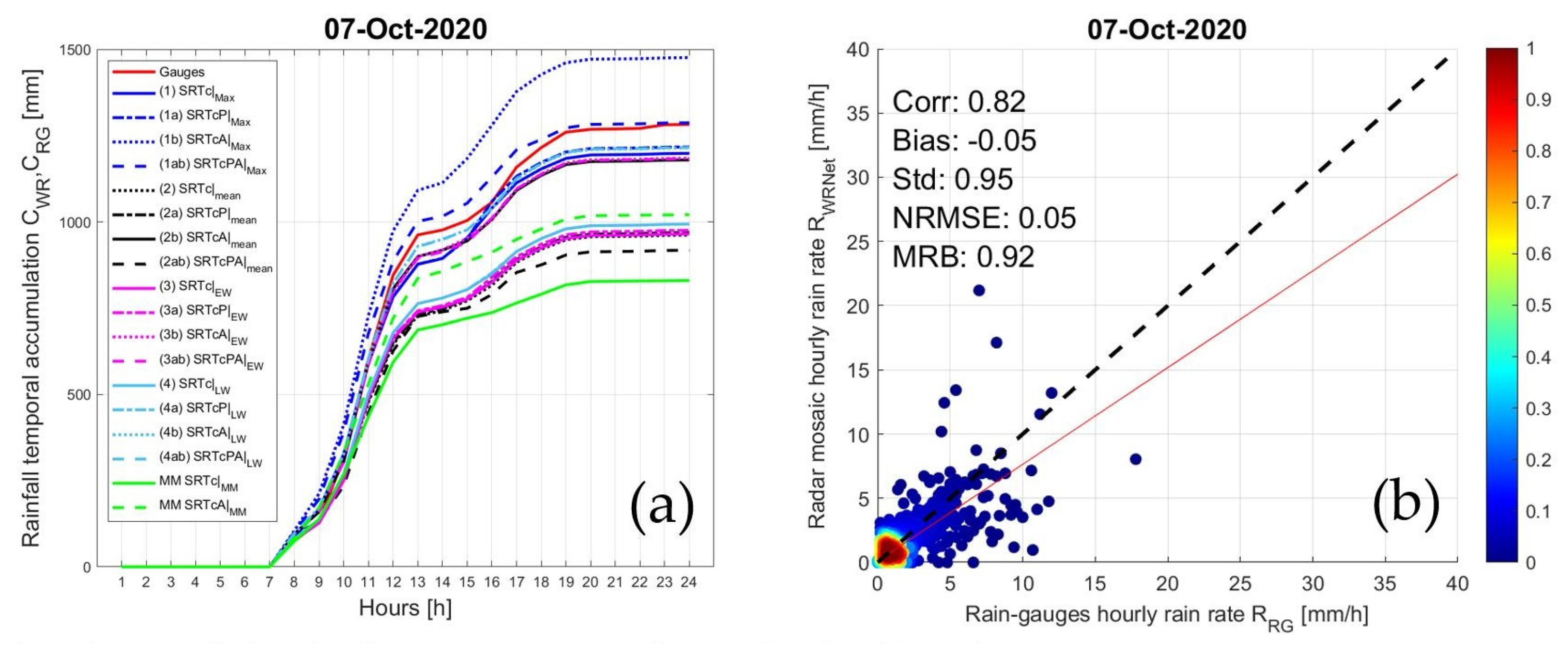
- Event on 7 October 2020. The third case is a widespread event during which the transit of a cloudy system of Atlantic origin through the central Italian regions facilitated showers on the Apennine areas, scattered rains, and the possibility of thunderstorms in the hilly and coastal areas.
4.2. Analysis of Selected Case Studies
- -
- the rainfall temporal accumulation CWRNet(t) (in mm), also called surface rainfall total (SRT), of hourly radar-based estimates and the corresponding ones CRG(t) of rain-gauge hourly measurements for each mosaicking type of Table 4. In formulas we have:where t goes from the beginning till the end of the precipitation event.
- -
- the correlation diagram between hourly rain rate estimates RWRNet(x,y,t) (in mm/h) from weather radar mosaic and hourly rain rate measurements RRG(x,y,t) (in mm/h) from rain gauges.
4.3. Overall Statistical Error Analysis
5. Conclusions
Author Contributions
Funding
Institutional Review Board Statement
Informed Consent Statement
Data Availability Statement
Acknowledgments
Conflicts of Interest
Appendix A. Radar Advanced Multiband Processing (RAMP) Main Modules
Appendix A.1. Pre-Processing Correction
Appendix A.2. Partial Beam Blockage Correction
Appendix A.3. Path Attenuation Correction
Appendix A.4. Total Quality Information

| Quality Index | Source of Error | Note |
|---|---|---|
| Radar system technical parameters | It is static within the whole radar range as well as in time and takes into account several factors as in [29]. | |
| Non-meteorological echo | Pixels affected by non-meteorological echoes are removed; for the uncertain pixel a value of 0.5 is applied, and the other data are set to 1. | |
| Partial beam blocking | It is computed from the corrected data taking into account the PBB value as in [28]. | |
| Long-range measurement | This quality factor decreases with increasing the measurement distance from the radar; it is computed as in [45]. | |
| Rain path attenuation | It is computed from the corrected data taking into account the PIA value as in [28]. | |
| Inhomogeneous vertical profile of reflectivity | The compensation of this effect is not performed in RAMP; the associated quality index is estimated as in [46]. |
Appendix A.5. Rainfall Rate Estimation
Appendix A.6. Vertically Integrated Liquid Estimation
Appendix A.7. Probability of Hail
Appendix A.8. Convective Storm Detection
Appendix A.9. Nowcasting
References
- Marzano, F.S.; Picciotti, E.; Vulpiani, G. Rain field and reflectivity vertical profile reconstruction from C-band radar volumetric data. IEEE Trans. Geosci. Remote Sens. 2004, 42, 1033–1046. [Google Scholar]
- Collier, C.G. Applications of weather radar systems. In A Guide to Uses of Radar Data in Meteorology and Hydrology; Wiley-Praxis: Chichester, UK, 1996; ISBN 0-7458-0510-8. [Google Scholar]
- Sauvageot, H. Radar Meteorology; Artech House: Norwood, NJ, USA, 1992. [Google Scholar]
- McKee, J.L.; Binns, A.D. A review of gauge–radar merging methods for quantitative precipitation estimation in hydrology. Can. Water Resour. J. Rev. Can. Des Ressour. Hydriques. 2015, 41, 186–203. [Google Scholar] [CrossRef]
- Ochoa-Rodriguez, S.; Wang, L.-P.; Willems, P.; Onof, C. A Review of Radar-Rain Gauge Data Merging Methods and Their Potential for Urban Hydrological Applications. Water Resour. Res. 2019, 55, 6356–6391. [Google Scholar] [CrossRef]
- Wang, L.-P.; Ochoa-Rodríguez, S.; Simoes, N.; Onof, C.; Maksimović, C. Radar–raingauge data combination techniques: A revision and analysis of their suitability for urban hydrology. Water Sci. Technol. 2013, 68, 737–747. [Google Scholar] [CrossRef]
- Goudenhoofdt, E.; Delobbe, L. Evaluation of radar-gauge merging methods for quantitative precipitation estimates. Hydrol. Earth Syst. Sci. 2009, 13, 195–203. [Google Scholar] [CrossRef] [Green Version]
- Picciotti, E.M.; Montopoli, S.; Di Fabio, F.S. Marzano Statistical calibration of surface rain fields derived from C-band Mt. Midia operational radar in central Italy. In Proceedings of the ERAD 2010, Sibiu, Romania, 6–10 September 2010. [Google Scholar]
- Antonini, A.; Melani, S.; Corongiu, M.; Romanelli, S.; Mazza, A.; Ortolani, A.; Gozzini, B. On the Implementation of a Regional X-Band Weather Radar Network. Atmosphere 2017, 8, 25. [Google Scholar] [CrossRef] [Green Version]
- Huuskonen, A.; Saltikoff, E.; Holleman, I. The Operational Weather Radar Network in Europe. Bull. Am. Meteorol. Soc. 2014, 95, 897–907. [Google Scholar] [CrossRef]
- Junyent, F.V.; Chandrasekar, D.; McLaughlin, E.; Insanic, N.B. The CASA Integrated Project 1 Networked Radar System. J. Atmos. Ocean. Technol. 2010, 27, 61–78. [Google Scholar] [CrossRef]
- Maki, M.; Maesaka, T.; Kato, A.; Kim, D.S.; Iawanami, K. Developing a Composite Rainfall Map Based on Observations from an X-Band Polarimetric Radar Network and Conventional C-Band Rada; NISCAIR-CSIR: New Delhi, India, 2012; Volume 41, pp. 461–470. [Google Scholar]
- Michelson, D.; Henja, A.; Ernes, S.; Haase, G.; Koistinen, J.; Ośródka, K.; Peltonen, T.; Szewczykowski, M.; Szturc, J. BALTRAD Advanced Weather Radar Networking. J. Open Res. Softw. 2018, 6, 12. [Google Scholar] [CrossRef] [Green Version]
- Lengfeld, K.; Clemens, M.; Münster, H.; Ament, F. Performance of high-resolution X-band weather radar networks—The PATTERN example. Atmos. Meas. Tech. 2014, 7, 4151–4166. [Google Scholar] [CrossRef] [Green Version]
- Marzano, F.S.; Ronzoni, M.; Montopoli, M.; Di Fabio, S.; Picciotti, E.; Vulpiani, G. Statistical characterization of C-band single-polarization radar retrieval space-time error in complex orography. In Proceedings of the ERAD2012, Toulouse, France, 25–29 June 2012. [Google Scholar]
- Vulpiani, G.P.; Pagliara, M.; Negri, L.; Rossi, A.; Gioia, P.; Giordano, P.P.; Alberoni, R.; Cremonini, L.; Ferraris, F.S. Marzano, The Italian radar network within the national early-warning system for multi-risks management. In Proceedings of the ERAD08, Helsinki, Finland, 30 June–4 July 2008. [Google Scholar]
- Picciotti, E.; Marzano, F.S.; Anagnostou, E.N.; Kalogiros, J.; Fessas, Y.; Volpi, A.; Cazac, V.; Pace, R.; Cinque, G.; Bernardini, L.; et al. Coupling X-band dual-polarized mini-radars and hydro-meteorological forecast models: The HYDRORAD project. Nat. Hazards Earth Syst. Sci. 2013, 13, 1229–1241. [Google Scholar] [CrossRef] [Green Version]
- Charba, J.; Liang, F. Quality control of gridded national radar reflectivity data. In Proceedings of the 21st Conference on Weather Analysis and Forecasting/17th Conference on Numerical Weather Prediction, Washington, WA, USA, 5 August 2005. [Google Scholar]
- Picciotti, E.; Marzano, F.S.; Colaiuda, V.; Cinque, G.; Massabò, M.; Deda, M.; Campanella, P.; Abeti, A.; Sini, F.; Neri, C.A.; et al. The ADRIARadNet project: ADRIAtic integrated RADar-based and web-oriented information processing system NETwork to support hydrometeorological monitoring and civil protection decision. In Proceedings of the ERAD2014, Garmisch, Germany, 1–5 September 2014. [Google Scholar]
- Picciotti, E.; Marzano, F.S.; Cinque, G.; Iovino, A.; Rossi, F.; Molinari, F.; Tomljanović, M. Using X-band mini-radar network within the Decision Support System in the framework of the CapRadNet project. In Proceedings of the European Conference on Radar in Meteorology and Hydrology (ERAD2016), Antalya, Turkey, 10–14 October 2016. [Google Scholar]
- Jewell, S.A.; Gaussiat, N. An assessment of kriging-based rain-gauge-radar merging techniques. Q. J. R. Meteorol. Soc. 2015, 141, 2300–2313. [Google Scholar] [CrossRef]
- Nanding, N.; Rico-Ramirez, M.A.; Han, D. Comparison of different radar-raingauge rainfall merging techniques. J. Hydroinformatics 2015, 17, 422. [Google Scholar] [CrossRef]
- Thorndahl, S.; Nielsen, J.E.; Rasmussen, M.R. Bias adjustment and advection interpolation of long-term high resolution radar rainfall series. J. Hydrol. 2014, 508, 214–226. [Google Scholar] [CrossRef]
- Colli, M.; Lanza, L.G.; La Barbera, P.; Chan, P.W. Measurement accuracy of weighing and tipping-bucket rainfall intensity gauges under dynamic laboratory testing. Atmos. Res. 2014, 144, 186–194. [Google Scholar] [CrossRef]
- Hanachi, C.; Bénaben, F.; Charoy, F. The Dewetra Platform: A Multi-perspective Architecture for Risk Management during Emergencies. In Information Systems for Crisis Response and Management in Mediterranean Countries; Springer International Publishing: Cham, Switzerland, 2014; pp. 165–177. [Google Scholar]
- Lanza, L.G.; Leroy, M.; van der Meulen, J.; Ondrás, M. The WMO laboratory intercomparison of rainfall intensity gauges—Instruments and observing methods. Atmos. Res. 2009, 94, 534–543. [Google Scholar] [CrossRef]
- Vulpiani, G.; Montopoli, M.; Passeri, L.D.; Gioia, A.G.; Giordano, P.; Marzano, F.S. On the Use of Dual-Polarized C-Band Radar for Operational Rainfall Retrieval in Mountainous Areas. J. Appl. Meteor. Climatol. 2012, 51, 405–425. [Google Scholar] [CrossRef]
- Barbieri, S. Testing of Dual-Polarization Processing Algorithms for Radar Rainfall Estimation in Tropical Scenarios; HSAF, Visiting Scientist H_AS17_01 Report; EUMETSAT HSAF: Darmstadt, Germany, 2017; Available online: https://hsaf.meteoam.it/VisitingScientist (accessed on 5 November 2021).
- Osrodka, K.; Szturc, J.; Jurczyk, A. Chain of data quality algorithms for 3D single-polarization radar reflectivity (RADVOL-QC system). Meteorol. Appl. 2014, 21, 256–270. [Google Scholar] [CrossRef]
- Bringi, V.N.; Chandrasekar, V. Polarimetric Doppler Weather Radar: Principles and Applications; Cambridge University Press: Cambridge, UK, 2001. [Google Scholar]
- Marshall, J.S.; Palmer, W.M.K. The distribution of raindrops with size. J. Meteorol. 1948, 5, 165–166. [Google Scholar] [CrossRef]
- Hong, Y.; Gourley, J.J. Radar Hydrology: Principles, Models and Applications; CRC Press: Boca Raton, FL, USA, 2018; ISBN 9781138855366. [Google Scholar]
- Sebastianelli, S.; Russo, F.; Napolitano, F.; Baldini, L. On precipitation measurements collected by a weather radar and a rain gauge network. Nat. Hazards Earth Syst. Sci. 2013, 13, 605–623. [Google Scholar] [CrossRef] [Green Version]
- Chiles, J.-P.; Delfiner, P. Geostatistics. In Modeling Spatial Uncertainty; John Wiley & Sons: New Jersey, NJ, USA, 2012. [Google Scholar]
- Picciotti, E.; Barbieri, S.; Di Fabio, S.; De Sanctis, K.; Lidori, R.; Marzano, F.S. Regional Precipitation Mosaicking Using Multifrequency Weather Radar Network in Complex Orography. In Proceedings of the 2020 IEEE Radar Conference (RadarConf20), Florence, Italy, 21–25 September 2020; pp. 1–6. [Google Scholar]
- Lakshmanan, V.; Humphrey, T.W. A MapReduce Technique to Mosaic Continental-Scale Weather Radar Data in Real-time. IEEE J. Sel. Top. Appl. Earth Obs. Remote Sens. 2014, 7, 721–732. [Google Scholar] [CrossRef]
- Zhang, J.; Howard, K.; Gourley, J.J. Constructing Three-Dimensional Multiple-Radar Reflectivity Mosaics: Examples of Convective Storms and Stratiform Rain Echoes. J. Atmos. Ocean. Technol. 2004, 22, 30–42. [Google Scholar] [CrossRef]
- Einfalt, T.; Lobbrecht, A.; Leung, K.; Lempio, G. Preparation and evaluation of a Dutch-German radar composite to enhance precipitation information in border areas. J. Hydrol. Eng. 2012, 18, 2. [Google Scholar] [CrossRef] [Green Version]
- Montopoli, M.; Picciotti, E.; Baldini, L.; Di Fabio, S.; Marzano, F.S.; Vulpiani, G. Gazing inside a giant-hail-bearing Mediterranean supercell by dual-polarization Doppler weather radar. Atmos. Res. 2021, 264, 105852. [Google Scholar] [CrossRef]
- Barbieri, S.; Picciotti, E.; Montopoli, M.; Di Fabio, S.; Lidori, R.; Marzano, F.S.; Kalogiros, J.; Anagnostou, M.; Baldini, L. Intercomparison of dual-polarization X-band miniradar performances with reference radar systems at X and C band in Rome supersite. In Proceedings of the ERAD2014, Garmisch, Germany, 1–5 September 2014. [Google Scholar]
- Bech, J.; Codina, B.; Lorente, J.; Bebbington, D. The sensitivity of single polarization weather radar beam blockage correction to variability in the vertical refractivity gradient. J. Atmos. Ocean. Technol. 2003, 20, 845–855. [Google Scholar] [CrossRef] [Green Version]
- Gorgucci, E.; Chandrasekar, V. Evaluation of attenuation correction methodology for dual-polarization radars: Application to X-band systems. J. Atmos. Oceanic Technol. 2005, 22, 1195–1206. [Google Scholar] [CrossRef]
- Tabary, P.; Le Henaff, G.; Dupuy, P.; Parent du Chatelet, J.; Testud, J. Can we use polarimetric X-band radars for operational quantitative precipitation estimation in heavy rain regions? In Proceedings of the Weather Radar and Hydrology International Symposium, Grenoble, France, 10–15 March 2008. [Google Scholar]
- Gourley, J.J.; Tabary, P.; Parent du Chatelet, J. Empirical estimation of attenuation from differential propagation phase measurements at C.-band. J. Appl. Meteorol. Climatol. 2007, 46, 306–317. [Google Scholar] [CrossRef] [Green Version]
- Rinollo, A.; Vulpiani, G.; Puca, S.; Pagliara, P.; Kaňák, J.; Lábό, E.; Okon, Ł.; Roulin, E.; Baguis, P.; Cattani, E.; et al. Definition and impact of a quality index for radar-based reference measurements in the H-SAF precipitation product validation. Nat. Hazards Earth Syst. Sci. 2013, 13, 2695–2705. [Google Scholar] [CrossRef] [Green Version]
- Friedrich, K.; Hagen, M.; Einfalt, T. A quality control concept for radar reflectivity, polarimetric parameters, and Doppler velocity. J. Atmos. Ocean. Technol. 2006, 23, 865–887. [Google Scholar] [CrossRef] [Green Version]
- Maki, M.; Park, S.-G.; Bringi, V.N. Effect of Natural Variations in Rain drop size distributions on rain rate estimators of 3 cm wavelength polarimetric radar. J. Meteorol. Soc. Jpn. 2005, 83, 871–893. [Google Scholar] [CrossRef] [Green Version]
- Diederich, M.; Zhang, P.; Simmer, C.; Troemel, S. Use of Specific Attenuation for Rainfall Measurement at X-Band Radar Wavelengths. Part I: Radar Calibration and Partial Beam Blockage Estimation. J. Hydrometeorol. 2015, 16, 487–502. [Google Scholar] [CrossRef]
- Diederich, M.; Ryzhkov, A.; Simmer, C.; Troemel, S. Use of Specific Attenuation for Rainfall Measurement at X-Band Radar Wavelengths. Part II: Rainfall Estimates and Comparison with Rain Gauges. J. Hydrometeorol. 2015, 16, 503–516. [Google Scholar] [CrossRef]
- Zhang, J.; Tang, L.; Cocks, S.; Zhang, P.; Ryzhkov, A.; Howard, K.; Langston, C.; Kaney, B. A Dual-polarization Radar Synthetic QPE for Operations. J. Hydrometeorol. 2020, 21, 2507–2521. [Google Scholar] [CrossRef] [Green Version]
- Ryzhkov, A.; Zrnić, D.S. Radar polarimetry at S, C, and X bands: Comparative analysis and operational implications. In Proceedings of the 32nd Conference on Radar Meteor, Albuquerque, NM, USA, 22–29 October 2005. [Google Scholar]
- Brimelow, J.C.; Reuter, G.W.; Bellon, A.; Hudak, D. A radar-based methodology for preparing a severe thunderstorm climatology in central Alberta. Atmos. Ocean. 2004, 42, 13–22. [Google Scholar] [CrossRef] [Green Version]
- Holleman, I. Hail detection using single-polarization radar. In Scientific Report; KNMI: De Bilt, The Netherlands, 2001. [Google Scholar]
- Amburn, S.A.; Wolf, P.L. VIL Density as a hail indicator. Weather Forecast. 1997, 12, 473–478. [Google Scholar] [CrossRef] [Green Version]
- Capozzi, V.; Picciotti, E.; Mazzarella, V.; Marzano, F.S.; Budillon, G. Fuzzy-logic detection and probability of hail exploiting short-range X-band weather radar. Atmos. Res. 2018, 201, 17–33. [Google Scholar] [CrossRef]
- Steiner, M.; Houze, R.A., Jr.; Yuter, S.E. Climatological characterization of three-dimensional storm structure from operational radar and rain gauge data. J. Appl. Meteorol. 1995, 34, 1978–2007. [Google Scholar] [CrossRef]
- Montopoli, M.; Marzano, F.S.; Picciotti, E.; Vulpiani, G. Spatially-Adaptive Advection Radar Technique for Precipitation Mosaic Nowcasting. IEEE J. Sel. Top. Appl. Earth Obs. Remote Sens. 2012, 5, 874–884. [Google Scholar] [CrossRef]
- Kuglin, C.; Hines, D. The Phase Correlation Image Alignment Method. In Proceedings of the International Conference on Cybernetics and Society, New York, NY, USA, 3–5 September 1975; pp. 163–165. [Google Scholar]


| Name/Features | M. Midia (MM) | Tortoreto (TO) | Cepagatti (CE) |
|---|---|---|---|
| Owner | CFA | CFA | CFA |
| System model | DWSR-93C | WR-25XP | WR-10X |
| Manufacturer | Enterprise, USA | ELDES, IT | ELDES, IT |
| Latitude | 42.06° | 42.78° | 42.40° |
| Longitude | 13.18° | 13.94° | 14.14° |
| Height (a.s.l.) | 1710 m | 15 m | 50 m |
| Polarization | Single | Dual | Single |
| Frequency band | C | X | X |
| Doppler capability | Yes | Yes | No |
| Peak power | 250 kW | 25 kW | 10 kW |
| Beamwidth | 1.6° | 3.0° | 3.0° |
| Antenna gain | 40.5 dB | 35 dB | 35 dB |
| Description | Symbol |
|---|---|
| Vertical maximum of reflectivity. This product is useful for the quick surveillance of regions covered by the radar. | VMI |
| Convective storm detection. This product is aimed at distinguishing stratiform and convective precipitation. | CSD |
| Nowcasting. This product is aimed at a short-term forecast of convective cells’ motion. | NOW |
| These products estimate the ground instantaneous (SRI) and accumulated (SRT) rain over the radar coverage area. | SRI, SRT |
| Vertically integrated liquid. This product can be used as a measure of the potential for strong rainfall. | VIL |
| Probability of hail. This product is aimed at the detection of hail, which is one of the most dangerous weather phenomena. | POH |
| ID | Label | Multi-Radar Merging Method | Reference |
| 1 | Max | Assign to the common pixel the maximum value of the available measurements. | [37] |
| 2 | Avg | Assign to the common pixel the mean value of the available measurements. | [37] |
| 3 | Lin | Assign to the common pixel a value-weighted with the distance from the radars, using linear weighting functions. | [38] |
| 4 | Exp | Assign to the common pixel a value weighted with the distance from the radars, using exponential weighting functions. | [37] |
| ID | Label | Single-Radar Processing Method | ID LABEL |
| a | Pol | Polarimetric rain rate estimation applied to the polarimetric radar in Tortoreto (TO). | P |
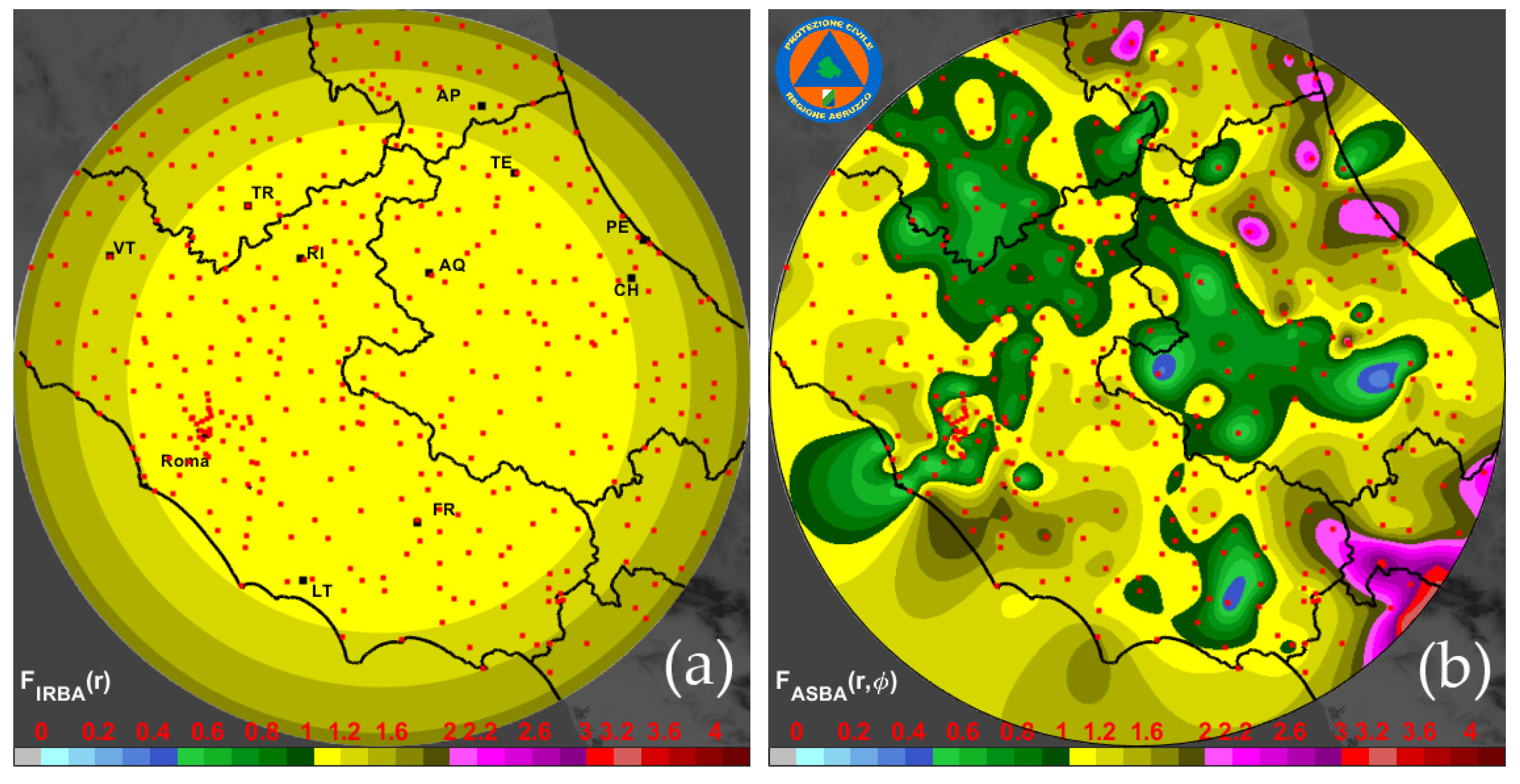
| b | Ani | Single-radar spatial anisotropic correction, based on the ASBA mapping (see Figure 4). | A |
| ID | Label | WR Network (WRN) Mosaicking Technique | ID LABEL |
| 1 | Max | Assign the maximum value among those covering the same grid of cells. | RWRN1 |
| 1a | MaxPol | Assign the maximum value among the available measurements. Polarimetric processing is performed on the TO-radar. | RWRN1a |
| 1b | MaxAni | Assign the maximum value among the available measurements after a single-radar spatial anisotropic correction. | RWRN1b |
| 1ab | MaxPolAni | Assign the maximum value among the available measurements. A single-radar spatial anisotropic correction and polarimetric processing on the TO-radar is performed. | RWRN1ab |
| 2 | Avg | Assign the mean value among those covering the same grid of cells. | RWR2 |
| 2a | AvgPol | Assign the mean value among the available measurements. Polarimetric processing on the TO-radar is performed. | RWRN2a |
| 2b | AvgAni | Assign the mean value among the available measurements after a single-radar spatial anisotropic correction. | RWRN2b |
| 2ab | AvgPol Ani | Assign the mean value among the available measurements. A single-radar spatial anisotropic correction and polarimetric processing on the TO-radar is performed. | RWRN2ab |
| 3 | Lin | Assign the value linear weighted with the distance from the radars among those covering the same grid of cells. | RWRN3 |
| 3a | LinPol | Assign the value linear weighted with the distance among the available measurements. Polarimetric processing is performed on the TO-radar. | RWRN3a |
| 3b | LinAni | Assign the value linear weighted with the distance among the available measurements after a single-radar spatial anisotropic correction. | RWRN3b |
| 3ab | LinPol Ani | Assign the value linear weighted with the distance among the available measurements. A single-radar spatial anisotropic correction and polarimetric processing on the TO-radar is performed. | RWRN3ab |
| 4 | Exp | Assign the value exponential weighted with the distance from the radars among those covering the same grid of cells. | RWRN4 |
| 4a | ExpPol | Assign the value exponential weighted with the distance among the available measurements. Polarimetric processing is performed on the TO-radar. | RWRN4a |
| 4b | ExpAni | Assign the value exponential weighted with the distance among the available measurements after a single-radar spatial anisotropic correction. | RWRN4b |
| 4ab | ExpPol Ani | Assign the value exponential weighted with the distance among the available measurements. A single-radar spatial anisotropic correction and polarimetric processing on the TO-radar is performed. | RWRN1b |
| Date | Atmospheric Phenomena | Precipitation Type | Duration (Day) | Maximum Rain Rate (mm/h) |
|---|---|---|---|---|
| 3 May 2018 | Rainstorm | Moderate/Frequent | 1 | 49 |
| 8 May 2018 | Rainstorm | Moderate/Frequent | 1 | 58 |
| 5 June 2018 | Storm | Light/Discontinuous | 1 | 41 |
| 8 June 2018 | Rainstorm | Moderate-heavy/Frequent | 1 | 61 |
| 22 June 2018 | Storm | Moderate/Frequent | 1 | 60 |
| 6 July 2018 | Rainstorm | Light/Discontinuous | 1 | 56 |
| 16 July 2018 | Rainstorm | Moderate/Frequent | 1 | 35 |
| 14 August 2018 | Rainstorm with hail | Intense/Persistent | 1 | 83 |
| 5 May 2019 | Rainstorm with snow/hail | Light/Discontinuous | 3 | 44 |
| 10 July 2019 | Rainstorm with hail | Intense/Persistent | 1 | 72 |
| 4 February 2020 | Rain and snow | Moderate/Frequent | 2 | 37 |
| 27 March 2020 | Rain and snow | Light/Discontinuous | 1 | 14 |
| 3 May 2020 | Rainstorm | Light/Discontinuous | 1 | 38 |
| 17 July 2020 | Rainstorm with hail | Light/Discontinuous | 1 | 42 |
| 7 October 2020 | Rainstorm with hail | Moderate/Discontinuous | 1 | 75 |
| 20 November 2020 | Rain and snow | Moderate/Frequent | 1 | 52 |
| ID | Corr Adim | Bias (mm/h) | STD (mm/h) | MAE (mm/h) | Nrmse Adim | FSE Adim | MRB Adim |
|---|---|---|---|---|---|---|---|
| 1 | 0.754 | −0.117 | 1.546 | 0.377 | 0.025 | 2.409 | 0.819 |
| 1a | 0.727 | −0.093 | 1.659 | 0.390 | 0.027 | 2.581 | 0.856 |
| 1b | 0.747 | 0.030 | 1.732 | 0.417 | 0.028 | 2.685 | 1.047 |
| 1ab | 0.713 | −0.0125 | 1.855 | 0.412 | 0.030 | 2.978 | 0.980 |
| 2 | 0.750 | −0.238 | 1.570 | 0.375 | 0.026 | 2.470 | 0.630 |
| 2a | 0.744 | −0.226 | 1.577 | 0.376 | 0.026 | 2.477 | 0.648 |
| 2b | 0.802 | −0.122 | 1.370 | 0.356 | 0.022 | 2.163 | 0.808 |
| 2ab | 0.677 | −0.251 | 1.680 | 0.418 | 0.027 | 2.749 | 0.594 |
| 3 | 0.740 | −0.253 | 1.587 | 0.373 | 0.026 | 2.509 | 0.605 |
| 3a | 0.733 | −0.241 | 1.594 | 0.373 | 0.026 | 2.515 | 0.624 |
| 3b | 0.760 | −0.155 | 1.511 | 0.356 | 0.025 | 2.361 | 0.759 |
| 3ab | 0.747 | −0.140 | 1.551 | 0.362 | 0.025 | 2.419 | 0.782 |
| 4 | 0.744 | −0.227 | 1.572 | 0.375 | 0.026 | 2.473 | 0.647 |
| 4a | 0.743 | −0.219 | 1.571 | 0.374 | 0.026 | 2.467 | 0.659 |
| 4b | 0.768 | −0.116 | 1.492 | 0.365 | 0.024 | 2.322 | 0.820 |
| 4ab | 0.765 | −0.108 | 1.501 | 0.367 | 0.024 | 2.333 | 0.833 |
| MM | 0.650 | −0.255 | 1.764 | 0.442 | 0.029 | 2.784 | 0.602 |
| MMa | 0.663 | −0.146 | 1.763 | 0.449 | 0.029 | 2.761 | 0.773 |
Publisher’s Note: MDPI stays neutral with regard to jurisdictional claims in published maps and institutional affiliations. |
© 2022 by the authors. Licensee MDPI, Basel, Switzerland. This article is an open access article distributed under the terms and conditions of the Creative Commons Attribution (CC BY) license (https://creativecommons.org/licenses/by/4.0/).
Share and Cite
Barbieri, S.; Di Fabio, S.; Lidori, R.; Rossi, F.L.; Marzano, F.S.; Picciotti, E. Mosaicking Weather Radar Retrievals from an Operational Heterogeneous Network at C and X Band for Precipitation Monitoring in Italian Central Apennines. Remote Sens. 2022, 14, 248. https://0-doi-org.brum.beds.ac.uk/10.3390/rs14020248
Barbieri S, Di Fabio S, Lidori R, Rossi FL, Marzano FS, Picciotti E. Mosaicking Weather Radar Retrievals from an Operational Heterogeneous Network at C and X Band for Precipitation Monitoring in Italian Central Apennines. Remote Sensing. 2022; 14(2):248. https://0-doi-org.brum.beds.ac.uk/10.3390/rs14020248
Chicago/Turabian StyleBarbieri, Stefano, Saverio Di Fabio, Raffaele Lidori, Francesco L. Rossi, Frank S. Marzano, and Errico Picciotti. 2022. "Mosaicking Weather Radar Retrievals from an Operational Heterogeneous Network at C and X Band for Precipitation Monitoring in Italian Central Apennines" Remote Sensing 14, no. 2: 248. https://0-doi-org.brum.beds.ac.uk/10.3390/rs14020248